A Bimodal Extension of the Epsilon-Skew-Normal Model

Abstract

This article introduces a bimodal model based on the epsilon-skew-normal distribution. This extension generates bimodal distributions similar to those produced by the mixture of normal distributions. We study the basic properties of this new family. We apply maximum likelihood estimators, calculate the information matrix and present a simulation study to assess parameter recovery. Finally, we illustrate the results to three real data sets, suggesting this new distribution as a plausible alternative for modelling bimodal data.

1. Introduction

In the last two decades of the twentieth century, inferential processes assumed the normality of the data. This assumption is not realistic in many cases, and the inferential processes were, therefore, inappropriate. In such situations, many authors decided to transform the variables in order to achieve symmetry or normality of the data, but these transformations led to unsatisfactory results because their interpretation became very complicated. Azzalini [1] introduced the skew-normal (SN) distribution, which allows asymmetric data to be modelled without the need for transformation. The probability density function (pdf) of the SN distribution is given by

$${\varphi }_{SN}(z;\lambda )=2\varphi \left(z\right)\Phi \left(\lambda z\right),z\in \mathbb{R},$$

(1)

where $\lambda \in \mathbb{R}$, $\varphi (·)$ and $\Phi (·)$ represent the pdf and cumulative distribution function (cdf) of the standard normal distribution, respectively. This is usually denoted by SN($\lambda$), where $\lambda$ is a shape parameter. Many works have since been published on the SN distribution. To name a few, Azzalini [2], Henze [3], Chiogna [4], Pewsey [5], Arellano-Valle et al. [6], DiCiccio and Monti [7], Salinas et al. [8], Rosco et al. [9], Shafiei and Doostparast [10], Adcock and Azzalini [11], etc.

Mudholkar and Hutson [12] studied the epsilon-skew-normal (ESN) distribution with an asymmetry parameter $\epsilon$, such that the standard normal distribution is recovered when $\epsilon =0$. Specifically, X has an ESN distribution if its pdf can be written as

$$g(x;\epsilon )=\varphi \left(\frac{x}{1-\mathrm{sgn}\left(x\right)\epsilon }\right)=\left\{\begin{array}{cc}\hfill \varphi \left(\frac{x}{1+\epsilon }\right),\hfill & \hfill \mathrm{if}x<0,\hfill \\ \hfill \varphi \left(\frac{x}{1-\epsilon }\right),\hfill & \hfill \mathrm{if}x\ge 0,\hfill \end{array}\right.$$

where sgn$(·)$ is the sign function and $-1<\epsilon <1$. We denote this by $X\sim ESN\left(\epsilon \right)$. The properties of this distribution were studied extensively by Mudholkar and Hutson [12]. Arellano-Valle et al. [13] introduced a general family of epsilon-skew-symmetric (ESS) distributions, of which the ESN distribution is a particular case. Some works using distributions of this family are as follows: Hansen [14] applied the epsilon-skew-t distribution to economic data; Gómez et al. [15] applied it to mining data; recently, Celis et al. [16] introduced an epsilon-positive family of distributions based on the ESS family and applied it to data with or without censoring and Bevilacqua et al. [17] used the ESS family for modelling atypical data in special statistics.

The SN and ESN distributions are unimodal, meaning that they are not appropriate in fields such as economics, health, engineering and many others where the data are often bimodal. One of the classic distributions used for modelling bimodal data is the mixture of the normal (MN) distribution, but it was criticised for identifiability problems. See, for example, McLachlan and Peel [18] and Marin et al. [19]. Despite the many innovations introduced in this area, the problem still persists in many cases, which is a disadvantage when working with models of this type. Hence researchers continue to develop new symmetric and asymmetric bimodal distributions.

Bimodal distributions have been obtained from this skew-symmetric model. For example, Azzalini and Capitanio [20], Ma and Genton [21], Arellano-Valle et al. [13], Kim [22], Elal-Olivero et al. [23], Arnold [24], Gómez et al. [25], Hassan and El-Bassiouni [26], da Silva et al. [27], Cordeiro et al. [28], da Braga et al. [29], Altun et al. [30] and Alizadeh et al. [31], among others. For further information on the results of SN distribution and related families, see Azzalini’s book [32].

Models of this type were studied by Kim [22], who introduced a bimodal extension of the SN model, named “two-pieces skew-normal model (TN)”, denoted by $TN\left(\lambda \right)$, whose pdf can be written as

$$g(z;\lambda )=c_{\lambda }\varphi \left(z\right)\Phi \left(\lambda \right|z\left|\right),z\in \mathbb{R},$$

(2)

where $\lambda \in \mathbb{R}$ and $c_{\lambda }=2\pi /(\pi +2arctan\left(\lambda \right))$. For $\lambda >0$, Kim [22] discusses that (2) defines a bimodal and symmetric around zero pdf.

An asymmetric extension of Kim’s model was presented by Arnold [24], who developed an asymmetric bimodal model named “the extended two-pieces skew-normal model (ETN)”, with pdf given by

$$h(z;\lambda ,\beta )=2c_{\lambda }\varphi \left(z\right)\Phi \left(\lambda \left|z\right|\right)\Phi \left(\beta z\right),z\in \mathbb{R},$$

(3)

where $\lambda ,\beta \in \mathbb{R}$ and $c_{\lambda }$ is a normalizing constant. The distribution is denoted by ETN($\lambda ,\beta$).

Another model widely applied in these situations is the MN distribution, which is given by:

$$f(x;{\mu }_1,{\sigma }_1,{\mu }_2,{\sigma }_2,p)=p\varphi (x;{\mu }_1,{\sigma }_1)+(1-p)\varphi (x;{\mu }_2,{\sigma }_2),x\in \mathbb{R},$$

where $\varphi (·;\mu ,\sigma )$ denotes the pdf of the normal distribution with parameters mean $\mu \in \mathbb{R}$ and standard deviation $\sigma \in {\mathbb{R}}^{+}$ and $0<p<1$.

This article is organised as follows: in Section 2, we give the pdf of the new distribution, its basic properties and moments; in Section 3, we make an inference by the maximum likelihood (ML) method, we calculate the information matrix and we carry out a simulation study to assess the properties of the ML estimators in finite samples; in Section 4, we show three fits to real data sets and compare them with other distributions, and in Section 5, we discuss some conclusions.

2. The New Density

In this section, we introduce the bimodal ESN (BESN) distribution, an extension of the ESN distribution and study its basic properties.

Definition 1. 

A random variable X has a BESN distribution if its pdf is given by

$$h(x;\epsilon ,\alpha )=\left(\frac{1+\alpha x^2}{1+(1+3{\epsilon }^2)\alpha }\right)\varphi \left(\frac{x}{1-sgn\left(x\right)\epsilon }\right),x\in \mathbb{R},$$

(4)

where $\left|\epsilon \right|<1$ and $\alpha \ge 0$. We denote this by $X\sim BESN(\epsilon ,\alpha )$.

Remark 1. 

Note that the BESN model contains the standard normal model when $\epsilon =\alpha =0$, while for $\alpha =0$, we obtain the ESN model. When $\epsilon =0$, we obtain a symmetric bimodal model considered in Elal-Olivero et al. [23]. Thus this model is a new alternative for modelling both symmetric and asymmetric bimodal data.

Proposition 1. 

If $X\sim BESN(\epsilon ,\alpha )$, $\left|\epsilon \right|<1$ and $\alpha \ge 0$, then its cdf is given by:

$$H(x;\epsilon ,\alpha )=\left\{\begin{array}{cc}\frac{(1+\epsilon )+\alpha {(1+\epsilon )}^3}{1+(1+3{\epsilon }^2)\alpha }\Phi \left(\frac{x}{1+\epsilon }\right)-\frac{\alpha x{(1+\epsilon )}^2}{1+(1+3{\epsilon }^2)\alpha }\varphi \left(\frac{x}{1+\epsilon }\right),\hfill & \hfill x<0,\\ \frac{(1+\epsilon )+\alpha {(1+\epsilon )}^3}{2\left[1+(1+3{\epsilon }^2)\alpha \right]}+\frac{1-\epsilon +\alpha {(1-\epsilon )}^3}{1+(1+3{\epsilon }^2)\alpha }\left[\Phi (\frac{x}{1-\epsilon }\right)-\frac{1}{2}]-\frac{\alpha x{(1-\epsilon )}^2}{1+(1+3{\epsilon }^2)\alpha }\varphi \left(\frac{x}{1-\epsilon }\right),\hfill & \hfill x\ge 0.\end{array}\right.$$

Remark 2. 

As expected, if $X\sim BESN(\epsilon ,\alpha )$, $\left|\epsilon \right|<1$, $\alpha \ge 0$, then

$$\underset{x\to \infty }{lim}H(x;\epsilon ,\alpha )=\frac{(1+\epsilon )+\alpha {(1+\epsilon )}^3}{2\left[1+(1+3{\epsilon }^2)\alpha \right]}+\frac{(1-\epsilon )+\alpha {(1-\epsilon )}^3}{2\left[1+(1+3{\epsilon }^2)\alpha \right]}=1.$$

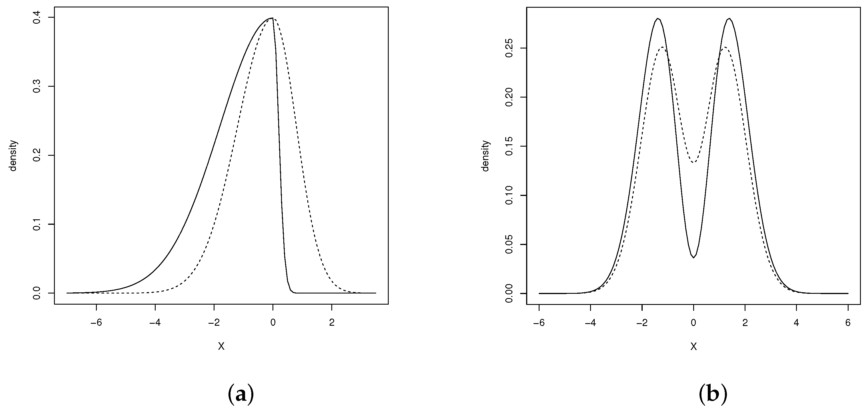
As can be seen from Figure 1, the shape of the pdf in relation to the unimodality and bimodality depends on parameters $\epsilon$ and $\alpha$.

Figure 1. Distributions (a) BESN(0.8,0) (solid line), BESN(0.2,0) (dashed line); (b) BESN(0,10) (solid line), BESN(0,2) (dashed line); (c) BESN(0.05,10) (solid line), BESN(0.05,2) (dashed line); and (d) BESN(0.2,4) (solid line), BESN(−0.2,4) (dashed line).

2.1. Properties

Proposition 2. 

Let $X\sim BESN(\epsilon ,\alpha )$. Then

(i) 

geometrically, $h(x;\epsilon ,\alpha )$ is a reflection of the ordinates related to the change in the sign of parameter ε. This is, $h(x;-\epsilon ,\alpha )=h(-x;\epsilon ,\alpha )$;

(ii) 

if $\epsilon =0$ then ${\displaystyle h(x;\alpha )=\frac{1+\alpha x^2}{1+\alpha }\varphi \left(x\right)}$, which is symmetric bimodal when $\alpha >1/2$ and symmetric unimodal if $\alpha \le 1/2$.

Proof. 

Using the density given in (4), the results are obtained immediately.    □

Proposition 3. 

Let $X\sim BESN(\epsilon ,\alpha )$. Then, the pdf for X is

1. 

bimodal when $\alpha >\frac{1}{2{(1-|\epsilon \left|\right)}^2}$ and its modes are located in

$$x_1=-\sqrt{\frac{2\alpha {(1+\epsilon )}^2-1}{\alpha }}and{x}_2=\sqrt{\frac{2\alpha {(1-\epsilon )}^2-1}{\alpha }}.$$

2. 

unimodal when $\epsilon \in (0,1)$ and

(a) 

$\frac{1}{2{(1+\epsilon )}^2}<\alpha <\frac{1}{2{(1-\epsilon )}^2}$, and its mode is located in $x=-\sqrt{\frac{2\alpha {(1+\epsilon )}^2-1}{\alpha }}.$

(b) 

$0\le \alpha \le \frac{1}{2{(1+\epsilon )}^2}$, and its mode is located in $x=0$.

3. 

unimodal when $\epsilon \in (-1,0)$ and

(a) 

$\frac{1}{2{(1-\epsilon )}^2}<\alpha <\frac{1}{2{(1+\epsilon )}^2}$, and its mode is located in $x=\sqrt{\frac{2\alpha {(1-\epsilon )}^2-1}{\alpha }}.$

(b) 

$0\le \alpha \le \frac{1}{2{(1-\epsilon )}^2}$, and its mode is located in $x=0$.

Proof. 

We calculate the first derivative of the pdf given in (4) and equal it to zero to find its critical values. That is,

$$h^{\prime }(x;\epsilon ,\alpha )=x\left(\frac{2\alpha }{1+\alpha x^2}-\frac{1}{{(1-\mathrm{sgn}\left(x\right)\epsilon )}^2}\right)h(x;\epsilon ,\alpha )=0.$$

Consequently, $x=0$ or $2\alpha -4\alpha \epsilon \mathrm{sgn}\left(x\right)+2\alpha {\epsilon }^2-1-\alpha x^2=0$. Without loss of generality, let us assume in the latter equation that $x>0$, hence we get the equation

$$2\alpha {(1-\epsilon )}^2-1-\alpha x^2=0,$$

(5)

then on solving it, we obtain that $x_2=\sqrt{\frac{2\alpha {(1-\epsilon )}^2-1}{\alpha }}$ whenever $\alpha >\frac{1}{2{(1-\epsilon )}^2}$. Now, assuming that $x<0$, we obtain the equation

$$2\alpha {(1+\epsilon )}^2-1-\alpha x^2=0,$$

(6)

then, as before, it follows that when $\alpha >\frac{1}{2{(1+\epsilon )}^2}$, then $x_1=-\sqrt{\frac{2\alpha {(1+\epsilon )}^2-1}{\alpha }}$, and so considering that $-1<\epsilon <1$ the proof of part 1 is concluded.

Considering the range of values of $\epsilon$ and $\alpha$ in 2(a), we can deduce that Equation (5) has no solution and that Equation (6) has a solution equal to $-\sqrt{(2\alpha {(1+\epsilon )}^2-1)/\alpha }$. Then, using the criterion of the second derivative for h, we have

$$\begin{array}{cc}\hfill h^{″}\left(-\sqrt{\frac{2\alpha {(1+\epsilon )}^2-1}{\alpha }}\right)& \hfill =\left[2\alpha \frac{1-(2\alpha {(1+\epsilon )}^2-1)}{{(1+2\alpha {(1+\epsilon )}^2-1)}^2}-\frac{1}{2{(1+\epsilon )}^2}\right]h\left(-\sqrt{\frac{2\alpha {(1+\epsilon )}^2-1}{\alpha }}\right)\hfill \\ \hfill & \hfill =\frac{1}{{(1+\epsilon )}^2}\left(\frac{1}{\alpha {(1+\epsilon )}^2}-2\right)h\left(-\sqrt{\frac{2\alpha {(1+\epsilon )}^2-1}{\alpha }}\right)<0.\hfill \end{array}$$

Therefore, at $-\sqrt{\frac{2\alpha {(1+\epsilon )}^2-1}{\alpha }}$ is attained a maximum of h. In consequence, it corresponds to their mode, and thus, proof 2(a) follows. On the other hand, in case 2(b), their hypotheses imply that Equations (5) and (6) have no solutions. Hence, the unique critical point of h is zero. Consequently, its mode is located at $x=0$.

Proceeding analogously to the proof of 2, the proof of part 3 follows, and thus the proof is completed.    □

2.2. Moments

This subsection is devoted to presenting the r-th moment of the $BESN(\epsilon ,\alpha )$ model and its moment-generating function (mgf).

Proposition 4. 

If $X\sim BESN(\epsilon ,\alpha )$. Then for $r=1,2,\dots ,$ the r-th distributional moment is given by

$$\mathbb{E}\left(X^r\right)=\frac{2^{r/2}\Gamma \left(\frac{r+1}{2}\right)}{\sqrt{\pi }(1+\alpha +3{\epsilon }^2\alpha )}\left[C_{\epsilon }(r+1)+\alpha (r+1)C_{\epsilon }(r+3)\right],$$

where $\left|\epsilon \right|<1$, $\alpha \ge 0$ and $C_{\epsilon }\left(k\right)=\frac{{(1-\epsilon )}^k+{(-1)}^{k-1}{(1+\epsilon )}^k}{2}$.

Proof. 

Let $Y\sim ESN\left(\epsilon \right)$, then

$${\mu }_r=\mathbb{E}\left(X^r\right)=\frac{E\left(Y^r\right)+\alpha E\left(Y^{r+2}\right)}{1+\alpha +3{\epsilon }^2\alpha }.$$

Hence, the result is obtained using the moments of the ESN model (see [12]).   □

Corollary 1. 

Let $X\sim BESN(\epsilon ,\alpha )$. Then

$$\begin{array}{c}\hfill \mathbb{E}\left(X\right)=-\sqrt{\frac{2}{\pi }}\frac{2\epsilon (4\alpha {\epsilon }^2+4\alpha +1)}{1+(1+3{\epsilon }^2)\alpha },\mathbb{E}\left(X^2\right)=\sqrt{\frac{2}{\pi }}\frac{(3.76\alpha +3.76{\epsilon }^2+37.6\alpha {\epsilon }^2+1.88\alpha {\epsilon }^4+1.2533)}{1+(1+3{\epsilon }^2)\alpha },\hfill \\ \hfill \mathbb{E}\left(X^3\right)=-\sqrt{\frac{2}{\pi }}\frac{4(3\alpha +(10\alpha +2){\epsilon }^2+3\alpha {\epsilon }^4+2)}{1+(1+3{\epsilon }^2)\alpha },\mathbb{E}\left(X^4\right)=\frac{3(5\alpha +5(21\alpha +2){\epsilon }^2+5(35\alpha +1){\epsilon }^4+35\alpha {\epsilon }^6+1)}{1+(1+3{\epsilon }^2)\alpha }.\hfill \end{array}$$

The skewness ($\sqrt{{\beta }_1}$) and kurtosis (${\beta }_2$) coefficients can be computed as

$$\begin{array}{c}\hfill \sqrt{{\beta }_1}=\frac{{\mu }_3-3{\mu }_1{\mu }_2+2{\mu }_1^3}{{\left({\mu }_2-{\mu }_1^2\right)}^{3/2}}and{\beta }_2=\frac{{\mu }_4-4{\mu }_1{\mu }_3+6{\mu }_1^2{\mu }_2-3{\mu }_1^4}{{\left({\mu }_2-{\mu }_1^2\right)}^2},\end{array}$$

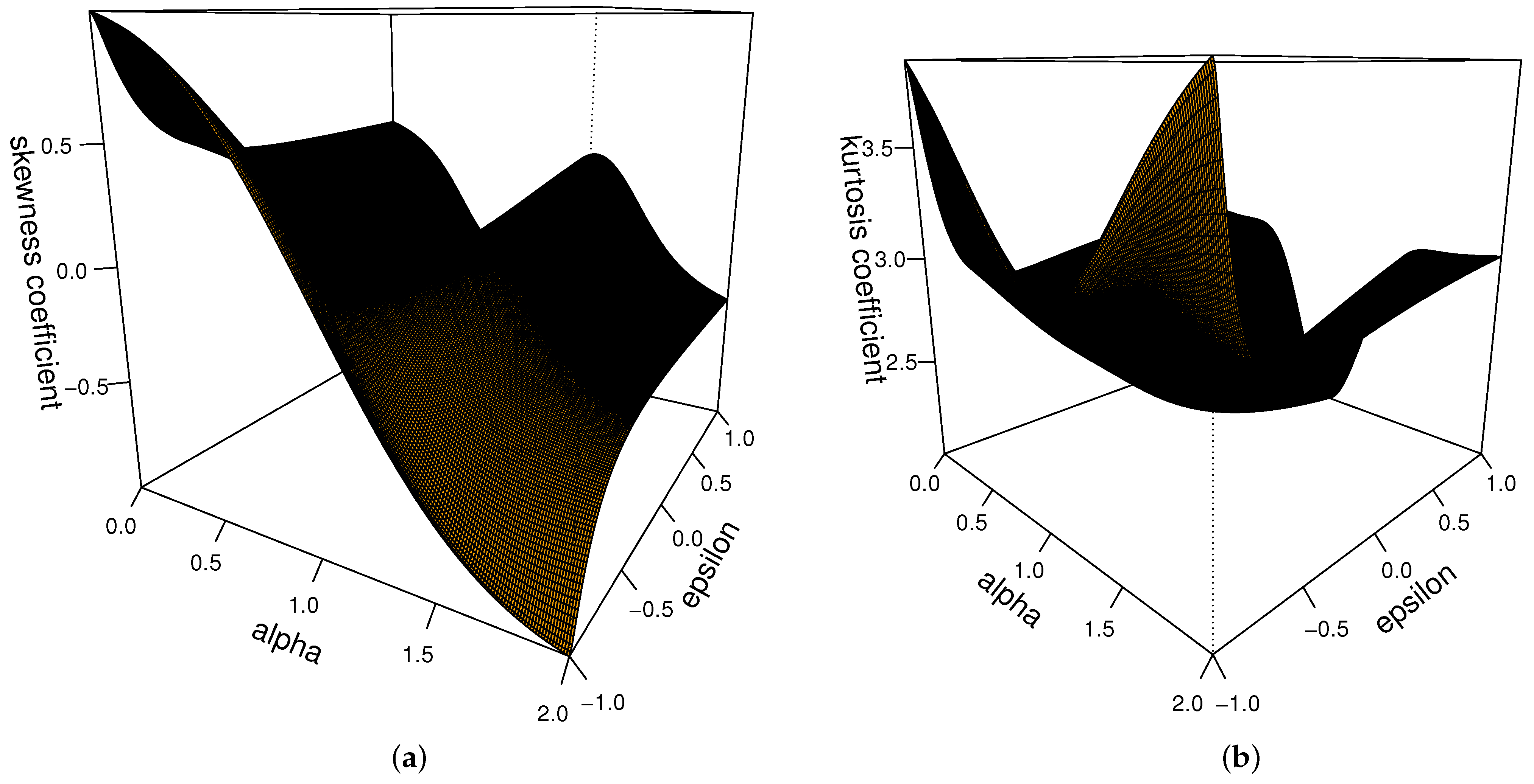
Figure 2 shows these coefficients for the BESN$(\epsilon ,\alpha )$ model in terms of $\epsilon$ and $\alpha$.

Figure 2. Plots for (a) skewness and (b) kurtosis coefficients for the BESN$(\epsilon ,\alpha )$ model.

Finally, in the following proposition, we present the mgf for the BESN distribution.

Proposition 5. 

The mgf for the $X\sim$BESN$(\epsilon ,\alpha )$ distribution is given by

$$\begin{array}{cc}\hfill M_X\left(t\right)& =\frac{(1+\epsilon )exp\left(\frac{t^2}{2}{(1+\epsilon )}^2\right)}{1+(1+3{\epsilon }^2)\alpha }\left[\Phi \left(t(1+\epsilon )\right)+{(1+\epsilon )}^2\left\{\left(1+t^2{(1+\epsilon )}^2\right)\Phi \left(t(1+\epsilon )\right)+t(1+\epsilon )\varphi \left(t(1+\epsilon )\right)\right\}\right]\hfill \\ \hfill & +\frac{(1-\epsilon )exp\left(\frac{t^2}{2}{(1-\epsilon )}^2\right)}{1+(1+3{\epsilon }^2)\alpha }\left[\Phi (-t(1-\epsilon ))+{(1-\epsilon )}^2\left\{\left(1+t^2{(1-\epsilon )}^2\right)\Phi (-t(1-\epsilon ))-t(1-\epsilon )\varphi \left(t(1-\epsilon )\right)\right\}\right].\hfill \end{array}$$

Proof. 

Using the definition $M_X\left(t\right)=\mathbb{E}\left(e^{tX}\right)$ and with a simple algebraic development, it is possible to obtain the result.    □

3. Inference

In this section, we apply the ML method to estimate the parameters. We calculate Fisher’s information matrix, and we carry out a simulation study.

3.1. ML Estimation

For a random sample $\mathbf{x}=(x_1,x_2,\dots ,x_n)$ of size n from the BESN distribution, the log-likelihood function for $\theta ={(\epsilon ,\alpha )}^{\top }$ is given by

$$\ell (\theta ;\mathbf{x})=\sum _{i=1}^{n}log(1+\alpha x^2)-\sum _{i=1}^{n}log(1+(1+3{\epsilon }^2)\alpha )-\frac{1}{2}\sum _{i=i}^n\frac{x_i^2}{{(1-\mathrm{sgn}\left(x_i\right)\epsilon )}^2}.$$

The score function is given by $U\left(\theta \right)={(U\left(ϵ\right),U\left(\alpha \right))}^{\top }$, where

$$\begin{array}{c}\hfill U(\epsilon )=-\frac{6\alpha \epsilon n}{1+(1+3{\epsilon }^2)\alpha }-\sum _{i=1}^n\frac{x_i^2\mathrm{sgn}\left(x_i\right)(1+\mathrm{sgn}\left(x_i\right)\epsilon )}{{(1-\mathrm{sgn}\left(x_i\right)\epsilon )}^3},\hfill \\ \hfill U(\alpha )=\sum _{i=1}^n\frac{x_i}{1+\alpha x_i^2}-n\frac{1+3{\epsilon }^2}{1+(1+3{\epsilon }^2)\alpha }.\hfill \end{array}$$

The ML estimators of $\alpha$ and $\epsilon$ are the solution of the system of equations $U\left(\theta \right)={\mathbf{0}}_2$, where ${\mathbf{0}}_p$ defines a vector of zeros with dimension p. The elements of the Hessian matrix, defined as the derivate of the score function with respect to each parameter, can be expressed as

$$\begin{array}{c}{U}_{\epsilon \alpha }=-\frac{6n\epsilon }{{(1+(1+3{\epsilon }^2)\alpha )}^2},U_{\epsilon \epsilon }=\frac{6{\epsilon }^2(3{\epsilon }^2-1)-6\alpha }{{(1+(1+3{\epsilon }^2)\alpha )}^2}-\sum _{i=1}^n\frac{3x_i^2}{{(1-\mathrm{sgn}\left(x_i\right)\epsilon )}^4},\hfill \\ U_{\alpha \alpha }=-\sum _{i=1}^n\frac{x_i^4}{{(1+\alpha x_i^2)}^2}-n\frac{{(1+3{\epsilon }^2)}^2}{{(1+(1+3{\epsilon }^2)\alpha )}^2}.\hfill \end{array}$$

3.2. Fisher’s Information Matrix

The elements of the Fisher’s information matrix are given by

$$\begin{array}{c}{I}_{\alpha \alpha }=\frac{1}{{\alpha }^2(1+(1+3{\epsilon }^2)\alpha )}\left[-1+1.2533\alpha (3+{\alpha }^2)\sqrt{\frac{2}{\pi }}+I_1+I_2\right]-\frac{{(1+3{\epsilon }^2)}^2}{{\left[(1+(1+3{\epsilon }^2)\alpha )\right]}^2}\hfill \\ I_{\alpha \epsilon }=\frac{6\epsilon }{{(1+(1+3{\epsilon }^2)\alpha )}^2},\hfill \\ I_{\epsilon \epsilon }=\frac{6\alpha [1-\alpha (3{\epsilon }^2-1)]}{{[1+(1+3{\epsilon }^2)\alpha ]}^2}+\frac{3}{1+(1+3{\epsilon }^2)\alpha }\left[3\alpha +0.62666\sqrt{\frac{2}{\pi }}\frac{2}{1-{\epsilon }^2}\right],\hfill \end{array}$$

where ${\displaystyle I_1={\int }_0^{\infty }\frac{1}{1+\alpha x^2}\varphi \left(\frac{x}{1+\epsilon }\right)dx=\frac{1}{2}\sqrt{\frac{\pi }{2\alpha }}\left[1-\Phi \left(\frac{1}{(1+\epsilon )\sqrt{2\alpha }}\right)\right]exp\left(\frac{1}{2\alpha {(1+\epsilon )}^2}\right)}$ and ${\displaystyle I_2={\int }_{-\infty }^0\frac{1}{1+\alpha x^2}\varphi \left(\frac{x}{1-\epsilon }\right)dx=-\frac{1}{2\sqrt{2\alpha }}exp\left(\frac{1}{2\alpha {(1-\epsilon )}^2}\right)\Gamma \left(\frac{1}{2},\frac{1}{2\alpha {(1-\epsilon )}^2}\right).}$ For more details of these integral formulas, we refer the reader to Gradshteyn and Ryzhik [33].

3.3. Location-Scale Case

For $Z\sim BESN(\epsilon ,\alpha )$, the extension to the location-scale case of the model follows from the transformation $X=\mu +\sigma Z$, where $\mu \in \mathbb{R}$ and $\sigma \in {\mathbb{R}}^{+}$. The pdf for X is given by

$$f(x;\mu ,\sigma ,\epsilon ,\alpha )=\frac{1+\alpha z^2}{\sigma (1+(1+3{\epsilon }^2)\alpha )}\varphi \left(\frac{z}{1-\mathrm{sgn}(x-\mu )\epsilon }\right),x\in \mathbb{R},$$

where $z=\frac{x-\mu }{\sigma }$. We denote this by $X\sim BESN(\mu ,\sigma ,\epsilon ,\alpha )$. Therefore, for a random sample $x_1,x_2,\dots ,x_n$ of the random variable $X\sim BESN(\mu ,\sigma ,\epsilon ,\alpha )$, the log-likelihood function for $\theta ={(\mu ,\sigma ,\epsilon ,\alpha )}^{\prime }$ is given by

$$\ell (\theta ;x)=\sum _{i=1}^{n}log(1+\alpha z_i^2)-nlog\left(\sigma [1+(1+3{\epsilon }^2)\alpha ]\right)-\frac{1}{2}\sum _{i=1}^n\frac{z_i^2}{{(1-\mathrm{sgn}(x_i-\mu )\epsilon )}^2},$$

where $z_i=\frac{x_i-\mu }{\sigma }$ and the score function can be expressed as

$$\begin{array}{c}U(\mu )=-\frac{2\alpha }{\sigma }\sum _{i=1}^n\frac{z_i}{1+\alpha z_i^2}+\frac{1}{\sigma }\sum _{i=1}^n\frac{z_i}{{[1-\mathrm{sgn}\left(x_i\right)\epsilon ]}^2},\hfill \\ U(\sigma )=-\frac{n}{\sigma }-\frac{2\alpha }{\sigma }\sum _{i=1}^n\frac{z_i^2}{1+\alpha z_i^2}+\frac{1}{\sigma }\sum _{i=1}^n\frac{z_i^2}{{[1-\mathrm{sgn}\left(x_i\right)\epsilon ]}^2},\hfill \\ U(\epsilon )=-\frac{6n\alpha \epsilon }{1+(1+3{\epsilon }^2)\alpha }-\sum _{i=1}^n\frac{z_i^2\mathrm{sgn}\left(x_i\right)}{{(1-\mathrm{sgn}\left(x_i\right)\epsilon )}^3},\hfill \\ U(\alpha )=\sum _{i=1}^n\frac{z_i^2}{1+\alpha z_i^2}-n\frac{1+3{\epsilon }^2}{1+(1+3{\epsilon }^2)\alpha }.\hfill \end{array}$$

The maximum likelihood estimator for $\theta$, say $\widehat{\theta }$, satisfies the asymptotic distribution

$$\sqrt{n}(\widehat{\theta }-\theta )\stackrel{\mathbf{L}}{⟶}{N}_4({\mathbf{0}}_4,I_F{\left(\theta \right)}^{-1}),asn\to +\infty ,$$

where $I_F\left(\theta \right)$ denotes the Fisher’s information matrix. See Appendix A for details about this matrix. In other words, $\widehat{\theta }$ is asymptotically normally distributed and consistent.

3.4. Simulation Study

In this subsection, we present a simulation study in order to assess the performance of the ML estimator in finite samples. To do this, Table 1, Table 2 and Table 3 consider three values for $\epsilon$: −0.90, −0.25 and 0.75; three values for $\alpha$: 0.5, 1.5 and 3; two values for $\mu$: −3 and 0; two values for $\sigma$: 1 and 5. Previous studies (not presented here) suggest that with smaller sample sizes (for example, $n=20$ and $n=50$), the estimators do not give good results in terms of bias; we, therefore, considered the following sample sizes: 100, 200 and 300. Values for the BESN distribution can be drawn using the Metropolis–Hastings algorithm. We use a burn-in period of 1000 and a thin of 20 in order to avoid a possible correlation between successive values. For each combination of $\epsilon$, $\alpha$, $\mu$, $\sigma$ and n (totaling 108 combinations), we draw 1000 samples of size n from the BESN$(\epsilon ,\alpha ,\mu ,\sigma )$ model, and for each, we compute the corresponding ML estimators. We report the bias of the 1000 samples, the mean of the estimated standard errors (SE) and the root of the estimated mean squared error (RMSE). In general terms, we note that the bias and the RMSE of the estimators decrease to zero when the sample size is increased, suggesting that the estimators are consistent even in finite samples. In addition, the SE and RMSE terms are closer when the sample size is increased, suggesting that the variance of the estimators is well estimated. However, as mentioned above, we suggest a sample size of at least approximately 100 data to ensure good properties of the maximum likelihood estimators.

Table 1. Recovery parameters for the ML estimators in the BESN model: case $\epsilon =-0.90$.

Real Value					$\mathit{n}=100$			$\mathit{n}=200$			$\mathit{n}=300$
$\mathit{\epsilon }$	$\mathit{\alpha }$	$\mathit{\mu }$	$\mathit{\sigma }$	Estimator	Bias	SE	RMSE	Bias	SE	RMSE	Bias	SE	RMSE
−0.90	0.5	−3	1	$\epsilon$	0.0541	0.0905	0.1014	0.0216	0.0622	0.0712	0.0114	0.0513	0.0643
				$\alpha$	−0.0464	0.2109	0.2328	−0.0257	0.1579	0.1628	−0.0159	0.1312	0.1345
				$\mu$	0.1590	0.1598	0.2770	0.0712	0.1132	0.1732	0.0469	0.0947	0.1545
				$\sigma$	0.0211	0.0731	0.0782	0.0098	0.0479	0.0485	0.0061	0.0385	0.0407
			5	$\epsilon$	0.0547	0.0908	0.1010	0.0213	0.0619	0.0706	0.0102	0.0510	0.0625
				$\alpha$	−0.0448	0.2160	0.2556	−0.0161	0.1602	0.1610	−0.0120	0.1318	0.1369
				$\mu$	0.7044	0.7975	1.2697	0.3487	0.5593	0.8595	0.2203	0.4636	0.7437
				$\sigma$	0.1182	0.3688	0.3928	0.0294	0.2367	0.2486	0.0122	0.1925	0.1977
		0	1	$\epsilon$	0.0535	0.0898	0.1003	0.0265	0.0636	0.0735	0.0123	0.0521	0.0614
				$\alpha$	−0.0482	0.2116	0.2398	−0.0134	0.1617	0.1678	−0.0104	0.1318	0.1324
				$\mu$	0.1666	0.1577	0.2714	0.0813	0.1157	0.1806	0.0452	0.0951	0.1424
				$\sigma$	0.0151	0.0740	0.0794	0.0077	0.0479	0.0524	0.0047	0.0383	0.0418
			5	$\epsilon$	0.0575	0.0915	0.1055	0.0218	0.0621	0.0733	0.0150	0.0530	0.0632
				$\alpha$	−0.0238	0.2293	0.3624	−0.0201	0.1595	0.1784	−0.0045	0.1344	0.1420
				$\mu$	0.7140	0.8185	1.2796	0.3623	0.5643	0.8962	0.2487	0.4873	0.7200
				$\sigma$	0.0999	0.3651	0.3861	0.0459	0.2405	0.2639	0.0060	0.1908	0.1948
	1.5	−3	1	$\epsilon$	0.1528	0.1315	0.2161	0.0673	0.0901	0.1182	0.0457	0.0721	0.0983
				$\alpha$	0.6421	1.8058	2.3750	−0.0288	0.6297	0.9154	−0.1046	0.4673	0.5272
				$\mu$	0.3700	0.2452	0.5209	0.1841	0.1638	0.3007	0.1375	0.1344	0.2548
				$\sigma$	−0.0059	0.0611	0.0586	0.0003	0.0419	0.0402	−0.0009	0.0335	0.0333
			5	$\epsilon$	0.1724	0.1338	0.2303	0.0749	0.0952	0.1305	0.0457	0.0739	0.0968
				$\alpha$	0.8948	2.0017	2.4838	0.0003	0.6613	0.9471	−0.0691	0.4888	0.5838
				$\mu$	1.7962	1.2963	2.6372	0.9216	0.8871	1.6184	0.6462	0.6871	1.2344
				$\sigma$	0.0135	0.3073	0.2903	0.0147	0.2109	0.1958	0.0055	0.1689	0.1679
		0	1	$\epsilon$	0.1534	0.1331	0.2125	0.0702	0.0933	0.1287	0.0455	0.0742	0.0954
				$\alpha$	0.6872	1.7292	2.2382	−0.0661	0.6044	0.8916	−0.1120	0.4661	0.5036
				$\mu$	0.3669	0.2454	0.5100	0.2036	0.1705	0.3454	0.1343	0.1390	0.2413
				$\sigma$	−0.0036	0.0610	0.0583	−0.0006	0.0421	0.0408	−0.0007	0.0336	0.0324
			5	$\epsilon$	0.1738	0.1353	0.2314	0.0763	0.0915	0.1353	0.0429	0.0732	0.0957
				$\alpha$	0.7678	1.8245	2.2004	−0.0427	0.5958	0.7176	−0.0567	0.4996	0.6068
				$\mu$	1.8173	1.3049	2.6672	0.9735	0.8537	1.7009	0.6193	0.6783	1.2289
				$\sigma$	0.0136	0.3072	0.2797	0.0036	0.2087	0.1970	0.0013	0.1685	0.1589
	3.0	−3	1	$\epsilon$	0.1961	0.1435	0.2314	0.1053	0.1071	0.1457	0.0693	0.0894	0.1061
				$\alpha$	1.4964	5.3344	4.2244	0.3920	2.3591	2.8872	0.1161	1.6347	2.1301
				$\mu$	0.4463	0.2795	0.5629	0.2593	0.1995	0.3697	0.1786	0.1648	0.2741
				$\sigma$	−0.0107	0.0629	0.0594	−0.0035	0.0441	0.0417	−0.0013	0.0358	0.0337
			5	$\epsilon$	0.1977	0.1403	0.2333	0.1092	0.1110	0.1466	0.0719	0.0895	0.1137
				$\alpha$	1.4941	5.2189	4.0158	0.5692	2.6032	3.0761	0.1230	1.7002	2.2917
				$\mu$	2.1036	1.3869	2.7459	1.2354	1.0343	1.7933	0.8910	0.8250	1.4584
				$\sigma$	−0.0196	0.3170	0.2962	−0.0074	0.2235	0.2015	0.0006	0.1795	0.1634
		0	1	$\epsilon$	0.1894	0.1384	0.2244	0.1105	0.1072	0.1519	0.0709	0.0903	0.1096
				$\alpha$	1.5907	5.5898	4.4033	0.3383	2.4152	3.1410	0.0662	1.6356	2.1862
				$\mu$	0.4310	0.2712	0.5437	0.2721	0.2013	0.3856	0.1800	0.1657	0.2833
				$\sigma$	−0.0100	0.0628	0.0604	−0.0037	0.0442	0.0417	−0.0015	0.0359	0.0331
			5	$\epsilon$	0.1983	0.1417	0.2340	0.1024	0.1114	0.1407	0.0740	0.0890	0.1143
				$\alpha$	1.6900	5.6618	4.3236	0.5178	2.4453	2.8307	0.0887	1.6908	2.4463
				$\mu$	2.0904	1.3993	2.7472	1.1472	1.0206	1.7184	0.9137	0.8326	1.4344
				$\sigma$	−0.0161	0.3176	0.2769	0.0074	0.2249	0.2038	−0.0040	0.1788	0.1642

Table 2. Recovery parameters for the ML estimators in the BESN: case $\epsilon =-0.25$.

Real Value					$\mathit{n}=100$			$\mathit{n}=200$			$\mathit{n}=300$
$\mathit{\epsilon }$	$\mathit{\alpha }$	$\mathit{\mu }$	$\mathit{\sigma }$	Estimator	Bias	SE	RMSE	Bias	SE	RMSE	Bias	SE	RMSE
−0.25	0.5	−3	1	$\epsilon$	−0.0157	0.1529	0.2479	0.0001	0.1297	0.2025	0.0100	0.1198	0.1708
				$\alpha$	0.1564	0.3744	0.5107	0.0832	0.2422	0.3204	0.0585	0.1948	0.2567
				$\mu$	0.0085	0.4244	0.7207	0.0352	0.3873	0.6177	0.0429	0.3660	0.5381
				$\sigma$	−0.0114	0.1068	0.1043	−0.0017	0.0700	0.0783	0.0012	0.0572	0.0638
			5	$\epsilon$	0.0004	0.1541	0.2454	0.0065	0.1313	0.2090	−0.0005	0.1187	0.1746
				$\alpha$	0.2217	0.4080	0.5995	0.1074	0.2494	0.3463	0.0514	0.1896	0.2447
				$\mu$	0.2216	2.1574	3.6385	0.2827	1.9646	3.2013	0.0941	1.7944	2.6873
				$\sigma$	−0.0562	0.5363	0.5480	−0.0289	0.3470	0.3834	−0.0070	0.2787	0.3263
		0	1	$\epsilon$	−0.0074	0.1511	0.2502	0.0069	0.1317	0.2034	0.0040	0.1195	0.1751
				$\alpha$	0.1851	0.3825	0.5663	0.0863	0.2432	0.3162	0.0450	0.1906	0.2427
				$\mu$	0.0294	0.4230	0.7286	0.0534	0.3932	0.6136	0.0366	0.3619	0.5402
				$\sigma$	−0.0128	0.1010	0.1047	−0.0042	0.0694	0.0727	0.0011	0.0585	0.0690
			5	$\epsilon$	−0.0027	0.1522	0.2416	−0.0031	0.1320	0.1954	0.0063	0.1213	0.1788
				$\alpha$	0.1754	0.3899	0.5729	0.0780	0.2457	0.3367	0.0475	0.1931	0.2444
				$\mu$	0.2365	2.1344	3.5399	0.1097	1.9540	3.0006	0.2116	1.8432	2.7743
				$\sigma$	−0.0399	0.5551	0.5357	−0.0038	0.3768	0.4089	−0.0110	0.2813	0.2984
	1.5	−3	1	$\epsilon$	−0.0029	0.0909	0.1336	−0.0017	0.0686	0.0834	−0.0044	0.0554	0.0602
				$\alpha$	0.5873	1.0765	1.4033	0.2078	0.5539	0.6239	0.1430	0.4278	0.4549
				$\mu$	0.0027	0.3000	0.4507	−0.0015	0.2353	0.2782	−0.0095	0.1917	0.2066
				$\sigma$	−0.0150	0.0627	0.0677	−0.0066	0.0451	0.0476	−0.0044	0.0371	0.0373
			5	$\epsilon$	−0.0032	0.0959	0.1343	−0.0011	0.0685	0.0786	−0.0022	0.0567	0.0606
				$\alpha$	0.4922	1.0005	1.2341	0.2218	0.5600	0.6518	0.1111	0.4181	0.4243
				$\mu$	0.0001	1.5904	2.2516	0.0282	1.1777	1.3209	−0.0137	0.9821	1.0770
				$\sigma$	−0.0714	0.3232	0.3412	−0.0280	0.2262	0.2271	−0.0190	0.1861	0.1954
		0	1	$\epsilon$	−0.0036	0.0954	0.1166	−0.0033	0.0674	0.0847	0.0025	0.0553	0.0580
				$\alpha$	0.4390	0.9887	1.2058	0.2165	0.5557	0.6148	0.1343	0.4257	0.4539
				$\mu$	0.0046	0.3184	0.3861	−0.0044	0.2317	0.2869	0.0134	0.1916	0.2030
				$\sigma$	−0.0114	0.0637	0.0657	−0.0057	0.0451	0.0449	−0.0062	0.0371	0.0381
			5	$\epsilon$	0.0091	0.0920	0.1342	−0.0016	0.0696	0.0893	0.0027	0.0549	0.0594
				$\alpha$	0.5615	1.0813	1.4552	0.1850	0.5494	0.6107	0.1416	0.4272	0.4530
				$\mu$	0.2488	1.5197	2.2235	0.0122	1.1919	1.5179	0.0389	0.9491	1.0313
				$\sigma$	−0.0783	0.3203	0.3451	−0.0199	0.2275	0.2236	−0.0236	0.1855	0.1873
	3.0	−3	1	$\epsilon$	0.0003	0.0595	0.0638	0.0004	0.0413	0.0423	−0.0006	0.0333	0.0342
				$\alpha$	1.3145	2.9377	3.4302	0.5215	1.3653	1.6228	0.3349	1.0020	1.1052
				$\mu$	0.0130	0.1936	0.2141	0.0026	0.1360	0.1350	−0.0010	0.1098	0.1058
				$\sigma$	−0.0112	0.0560	0.0581	−0.0047	0.0399	0.0390	−0.0032	0.0325	0.0310
			5	$\epsilon$	0.0028	0.0603	0.0741	−0.0016	0.0413	0.0437	−0.0004	0.0335	0.0347
				$\alpha$	1.1584	2.8907	3.2538	0.5556	1.3965	1.7904	0.3435	1.0152	1.2337
				$\mu$	0.0774	0.9842	1.2218	−0.0150	0.6805	0.7274	0.0050	0.5528	0.5680
				$\sigma$	−0.0452	0.2817	0.3062	−0.0123	0.1996	0.1983	−0.0103	0.1631	0.1658
		0	1	$\epsilon$	−0.0015	0.0605	0.0639	−0.0031	0.0419	0.0453	0.0003	0.0332	0.0354
				$\alpha$	1.1992	2.8189	3.1728	0.5211	1.3798	1.7697	0.3652	1.0194	1.1536
				$\mu$	0.0080	0.1981	0.2161	−0.0040	0.1384	0.1400	0.0037	0.1093	0.1152
				$\sigma$	−0.0064	0.0563	0.0612	−0.0042	0.0400	0.0411	−0.0037	0.0325	0.0323
			5	$\epsilon$	0.0011	0.0598	0.0742	−0.0014	0.0417	0.0434	0.0005	0.0333	0.0337
				$\alpha$	1.1985	2.8208	3.0717	0.5648	1.4367	1.9708	0.3438	1.0043	1.1392
				$\mu$	0.0291	0.9731	1.2611	0.0306	0.6880	0.6916	0.0224	0.5496	0.5347
				$\sigma$	−0.0457	0.2812	0.2978	−0.0222	0.1997	0.2049	−0.0130	0.1629	0.1613

Table 3. Recovery parameters for the ML estimators in the BESN: case $\epsilon =0.75$.

Real Value					$\mathit{n}=100$			$\mathit{n}=200$			$\mathit{n}=300$
$\mathit{\epsilon }$	$\mathit{\alpha }$	$\mathit{\mu }$	$\mathit{\sigma }$	Estimator	Bias	SE	RMSE	Bias	SE	RMSE	Bias	SE	RMSE
0.75	0.5	−3	1	$\epsilon$	−0.0261	0.1149	0.1428	0.0067	0.0875	0.1095	0.0141	0.0742	0.0999
				$\alpha$	0.0140	0.2516	0.3032	0.0060	0.1739	0.1794	0.0085	0.1412	0.1548
				$\mu$	−0.1269	0.2405	0.3650	−0.0273	0.1836	0.2554	−0.0020	0.1564	0.2182
				$\sigma$	0.0030	0.0744	0.0802	−0.0058	0.0493	0.0511	−0.0046	0.0399	0.0433
			5	$\epsilon$	−0.0245	0.1157	0.1424	0.0085	0.0863	0.1126	0.0145	0.0736	0.0970
				$\alpha$	0.0145	0.2603	0.3996	0.0004	0.1714	0.1990	0.0042	0.1395	0.1476
				$\mu$	−0.6172	1.1996	1.7918	−0.1404	0.9037	1.3038	−0.0198	0.7727	1.0555
				$\sigma$	0.0222	0.3843	0.4149	−0.0070	0.2500	0.2842	−0.0243	0.1988	0.2222
		0	1	$\epsilon$	−0.0246	0.1131	0.1400	0.0017	0.0868	0.1109	0.0065	0.0744	0.1019
				$\alpha$	0.0197	0.2682	0.4594	0.0097	0.1750	0.2013	0.0085	0.1422	0.1598
				$\mu$	−0.1257	0.2329	0.3677	−0.0400	0.1828	0.2608	−0.0172	0.1578	0.2368
				$\sigma$	0.0055	0.0763	0.0823	−0.0019	0.0493	0.0543	−0.0022	0.0402	0.0460
			5	$\epsilon$	−0.0310	0.1202	0.1425	0.0037	0.0858	0.1153	0.0139	0.0749	0.1003
				$\alpha$	0.0132	0.2543	0.3580	0.0066	0.1716	0.1807	0.0003	0.1393	0.1444
				$\mu$	−0.6514	1.2586	1.8396	−0.1800	0.8930	1.3635	−0.0203	0.7925	1.1059
				$\sigma$	0.0271	0.3842	0.4040	−0.0179	0.2456	0.2661	−0.0151	0.2004	0.2093
	1.5	−3	1	$\epsilon$	−0.0699	0.1301	0.1703	−0.0257	0.1004	0.1269	−0.0097	0.0861	0.1094
				$\alpha$	0.5675	1.7173	2.3993	0.2243	0.8400	1.3474	0.1954	0.6693	1.1860
				$\mu$	−0.2456	0.2819	0.4944	−0.1079	0.2275	0.3477	−0.0625	0.1950	0.2956
				$\sigma$	−0.0180	0.0601	0.0645	−0.0074	0.0422	0.0439	−0.0081	0.0342	0.0373
			5	$\epsilon$	−0.0800	0.1307	0.1688	−0.0314	0.1041	0.1317	−0.0018	0.0857	0.1077
				$\alpha$	0.4805	1.5197	2.1254	0.1701	0.7780	1.1873	0.1937	0.7120	1.5127
				$\mu$	−1.2088	1.4375	2.2866	−0.6429	1.1896	1.8823	−0.2501	0.9625	1.3974
				$\sigma$	−0.0627	0.3014	0.3091	−0.0414	0.2119	0.2179	−0.0444	0.1709	0.1871
		0	1	$\epsilon$	−0.0814	0.1333	0.1736	−0.0277	0.1002	0.1272	−0.0114	0.0869	0.1102
				$\alpha$	0.3536	1.2198	1.5117	0.1569	0.7881	1.3050	0.1528	0.6086	0.9161
				$\mu$	−0.2658	0.2956	0.5000	−0.1250	0.2264	0.3568	−0.0656	0.1995	0.2901
				$\sigma$	−0.0183	0.0601	0.0648	−0.0093	0.0422	0.0443	−0.0088	0.0341	0.0363
			5	$\epsilon$	−0.0795	0.1325	0.1740	−0.0335	0.1029	0.1326	−0.0127	0.0871	0.1119
				$\alpha$	0.4461	1.4663	2.0314	0.1460	0.7606	1.2583	0.2174	0.7242	1.4759
				$\mu$	−1.2619	1.4768	2.4543	−0.6618	1.1716	1.8498	−0.3274	1.0096	1.4889
				$\sigma$	−0.0682	0.3014	0.3115	−0.0358	0.2121	0.2302	−0.0277	0.1725	0.1795
	3	−3	1	$\epsilon$	−0.0687	0.1302	0.1310	−0.0262	0.0996	0.1019	−0.0073	0.0826	0.0853
				$\alpha$	1.3821	4.9026	3.9807	0.8722	2.8543	3.3111	0.7448	2.2295	2.8217
				$\mu$	−0.2208	0.2764	0.3953	−0.1034	0.2195	0.3009	−0.0527	0.1875	0.2324
				$\sigma$	−0.0217	0.0611	0.0673	−0.0104	0.0443	0.0466	−0.0093	0.0365	0.0403
			5	$\epsilon$	−0.0763	0.1324	0.1448	−0.0263	0.0978	0.1049	−0.0061	0.0839	0.0895
				$\alpha$	1.1107	4.6872	4.0288	0.9511	3.0669	3.6594	0.7011	2.1487	2.7362
				$\mu$	−1.1417	1.4213	2.1190	−0.5647	1.0766	1.5742	−0.2584	0.9480	1.2493
				$\sigma$	−0.0695	0.3075	0.3168	−0.0587	0.2212	0.2465	−0.0451	0.1825	0.1965
		0	1	$\epsilon$	−0.0698	0.1325	0.1382	−0.0259	0.0987	0.1049	−0.0061	0.0833	0.0888
				$\alpha$	0.9497	4.3710	3.7766	0.7372	2.7392	3.2677	0.5977	1.9859	2.3943
				$\mu$	−0.2405	0.2806	0.4226	−0.1132	0.2180	0.3008	−0.0556	0.1878	0.2497
				$\sigma$	−0.0226	0.0610	0.0686	−0.0113	0.0442	0.0470	−0.0095	0.0364	0.0406
			5	$\epsilon$	−0.0848	0.1325	0.1587	−0.0277	0.1012	0.1036	−0.0107	0.0846	0.0891
				$\alpha$	0.8946	4.2192	3.6539	0.7349	2.7061	3.0920	0.6883	2.2972	3.1316
				$\mu$	−1.3457	1.4461	2.4238	−0.6004	1.1274	1.5485	−0.3252	0.9638	1.2807
				$\sigma$	−0.0928	0.3071	0.3216	−0.0670	0.2208	0.2401	−0.0474	0.1827	0.1982

4. Applications

In this section, we fit the BESN distribution to three real data sets that are widely used in the literature, namely the roller, birthweight and nickel data sets. The first application is to a unimodal data set and is compared with the fit of the normal (N) distribution; the second application is to a symmetric bimodal data set and is compared with the fits of the N and TN distributions; the third application is to an asymmetric bimodal data set and is compared with the fits of the SN, ETN and MN distributions. To compare the models, we use the Akaike information criterion AIC (see Akaike [34]) and the Bayesian information criterion BIC (see Schwarz [35]). Traditionally the preferred model is the one with the smallest AIC and/or BIC.

4.1. First Application: Roller Data

In this first application, we use the data set related to 1150 heights measured at 1-micron intervals along the drum of a roller (i.e., parallel to the axis of the roller). This was part of an extensive study of the surface roughness of the roller. It is available for downloading at http://lib.stat.cmu.edu/jasadata/laslett (accessed on 5 November 2022). Summary statistics for the data set are presented in Table 4.

Table 4. Summary statistics for the variable roller.

n	$\mathbf{Mean}$	S	${\mathit{b}}_1$	${\mathit{b}}_2$
1150	3.535	0.650	−0.986	4.855

Given the values of sample asymmetry, $b_1$, and sample kurtosis, $b_2$, there is strong evidence that an asymmetric model could provide a better fit to the data under study. Therefore, the N and BESN distributions are fitted to the data set.

The ML estimates for each model (N and BEST) and standard errors (SE) in parentheses are: $\widehat{\mu }=3.535\left(0.019\right)$ and $\widehat{\sigma }=0.650\left(0.014\right)$ with AIC$=2275.732$ and BIC$=2285.827$ for the N distribution and $\widehat{\mu }=4.944\left(0.034\right),$ $\widehat{\sigma }=0.495\left(0.011\right),$ $\widehat{\epsilon }=0.833\left(0.0348\right)$ and $\widehat{\alpha }=7.871\left(2.258\right)$ with AIC$=2181.560,$ and BIC$=2201.75$ for the BESN distribution.

According to AIC and BIC, the BESN distribution provides a better fit for the roller data set than the N distribution. In other words, the BESN distribution achieves a satisfactory fit for skewness and kurtosis, which is not adequately fitted by the N distribution. Therefore, the BESN distribution presents the best fit for the roller data set. A qq-plot for the variable roller, using normal and BESN distributions, is shown in Figure 3a,b.

Figure 3. QQ-plots fitted using (a) the N model, (b) the BESN model, (c) the cdf of the BESN model (dotted line) and empirical cdf (solid line).

Figure 3c shows the empirical cdf for the variable roller (solid line), while the dotted line corresponds to the cdf for the BESN model. The results suggest a better fit for the BESN model.

In addition, we also compare the N and BESN distributions with a hypothesis test. Specifically, we propose the hypothesis

$$H_{01}:(\epsilon ,\alpha )=(0,0)\mathrm{versus}{H}_{11}:(\epsilon ,\alpha )\ne (0,0),$$

which can be tested using the statistic

$${\Lambda }_1=\frac{{\ell }_N(\widehat{\mu },\widehat{\sigma })}{{\ell }_{BESN}(\widehat{\mu },\widehat{\sigma },\widehat{\epsilon },\widehat{\alpha })}.$$

After numerical evaluations, we obtain $-2log\left({\Lambda }_1\right)=96.172$, which is greater than the critical 5% chi-squared value with two degrees of freedom, namely ${\chi }_{2.95\%}^2=5.99$.

4.2. Second Application: Birthweight Data

In the second application, we study the fit of the BESN model to 500 units observed for the variable Z=b.weight, which is the ultrasound weight (birthweight in grams). These data are available as supplementary material. The summary statistics for the data set are presented in Table 5.

Table 5. Summary statistics for the variable birthweight.

n	Mean	S	${\mathit{b}}_1$	${\mathit{b}}_2$
500	3210	834.092	0.071	2.068

Given the symmetry of these data, we propose to fit a BESN model taking $\epsilon =0$ and then compare this with the fit of the N and TN models.

We used AIC and BIC to compare the fits of the N, TN and BESN models. According to these criteria (see Table 6 and Figure 4a), the BESN model is seen to present a better fit than the N and TN models.

Table 6. Parameter estimates and SE for the N, TN and BESN models.

Parameter	N	TN	BESN
$\mu$	3210.356 (37.301)	3207.422 (26.083)	3220.873 (26.947)
$\sigma$	834.092 (26.415)	772.688 (25.760)	555.235 (16.408)
$\alpha$	–	–	1.676 (0.368)
$\lambda$	–	1.771 (0.539)
AIC	8148.284	8109.672	8093.565
BIC	8156.713	8122.315	8106.208

Figure 4. (a) Histogram for the variable birthweight. Estimated pdf: N (dotted red line), TN (dashed blue line) and BESN (solid black line). (b) QQ-plot for the BESN distribution. (c) Empirical cdf for the variable birthweight (solid black line) and cdf of the BESN distribution (dotted red line).

Figure 4b,c show the qq-plot for the BESN model and the empirical cdf. The plots suggest a better fit for the BESN model than its competitors.

4.3. Third Application: Nickel Data

In this third application, we use a data set related to the logarithm of the nickel content in soil samples analysed at the Mines Department of Universidad de Atacama, Chile, which are available as supplementary material.

In this section, we compare the fits of the SN, BESN, ETN and MN models to the above data set.

The pdf for the MN model can be written as

$$f(x;{\xi }_1,{\sigma }_1,{\xi }_2,{\sigma }_2,p)=\frac{p}{{\sigma }_1}\varphi (x,{\xi }_1,{\sigma }_1)+\frac{1-p}{{\sigma }_2}\varphi (x;{\xi }_2,{\sigma }_2),x\in \mathbb{R},$$

with parameters $({\xi }_j,{\sigma }_j)\in \mathbb{R}\times {\mathbb{R}}^{+}$, $j=1,2$ and $0<p<1$, we denote as MN$({\xi }_1,{\sigma }_1,{\xi }_2,{\sigma }_2,p)$.

The comparisons are made using the AIC and BIC for the variable Y, the logarithm of the nickel concentration. In all cases, the parameters are estimated by ML using bbmle in the R software package [36]. The SE of the ML estimates is calculated using the observed information matrix corresponding to each model.

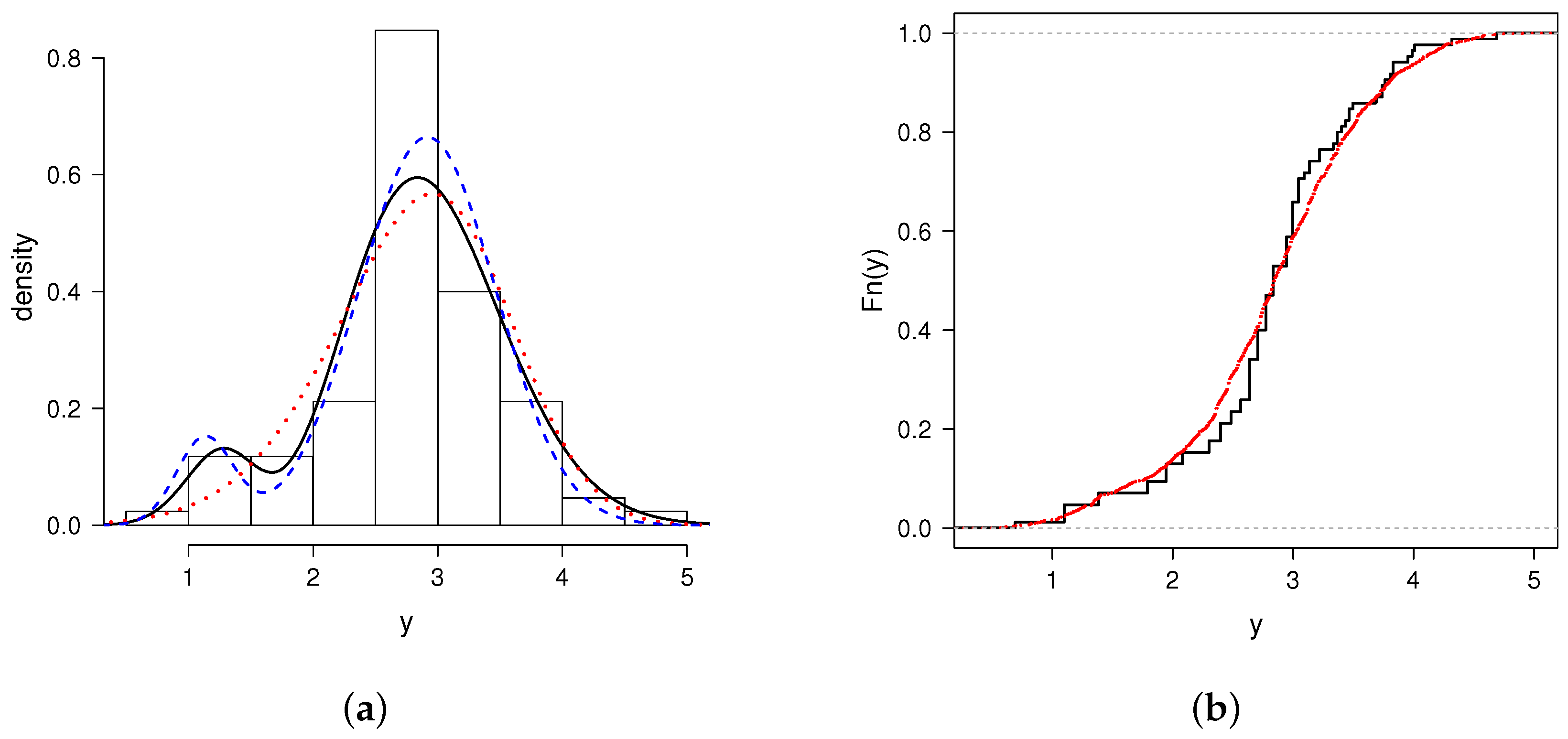
Table 7 gives the estimated parameters and AIC and BIC for the SN, ETN, BESN and MN models. The respective SE are in parentheses. The graph in Figure 5 shows that the BESN model presents quite a good fit.

Table 7. Estimated parameters and AIC and BIC for the SN, ETN, BESN and MN distributions. The respective SE are in parentheses.

Parameters	SN	ETN	BESN	Parameters	MN
$\xi$	3.4851 (0.1545)	2.1977( 0.0973)	1.6740 (0.1323)	${\xi }_1$	1.1320 (0.1094)
$\sigma$	0.9797 (0.1281)	0.9094 (0.0892)	0.5954 (0.0364)	${\sigma }_1$	0.2280 (0.0771)
$\epsilon$			4.0647(1.9118)	${\xi }_2$	2.9167(0.0640)
$\alpha$	−1.5950 (0.5872)	2.3479 (1.4204)	−0.4232 (0.0692)	${\sigma }_2$	0.5494 (0.0434)
$\beta$		1.1509 (0.2944)		p	0.0853 (0.0316)
AIC	190.198	190.768	186.3271		188.751
BIC	197.525	200.538	196.097		200.964

Figure 5. Fitted densities: (a) SN (dotted red line), MN (dashed blue line) and BESN (solid black line), (b) Empirical cdf (solid black line) and BESN distribution (dashed red line).

In all cases, the models are augmented by the inclusion of location ($\xi$) and scale ($\sigma$) parameters. Since the models are not nested, the AIC and BIC have been used to compare the distributions. According to these criteria, the BESN model provides the best fit to the data of the example. Hence, the BESN model seems to be a useful alternative for modelling the data for the logarithm of the nickel concentration.

The conclusion of the study is that the BESN model appears to be more appropriate for the particular data sets analysed here. These points are illustrated in more detail in Figure 5, where the histograms and the fitted curves for the data sets are displayed.

5. Final Comments

In this paper, we propose the BESN distribution, which is shown to have flexible modes. We study its properties and implement ML estimation. Some other characteristics of the BESN distribution are:

• The BESN distribution contains, as special cases, the N and ESN distributions.
• The BESN model is very flexible in its modes, as we discuss in Figure 1 and Figure 2; it can be used to fit both unimodal data (application 1), and bimodal data (applications 2 and 3).
• The BESN distribution has a closed expression for its cdf.
• The moments of the BESN distribution have a closed expression.
• The three applications show that the BESN distribution provides a better fit than the other models tested.

Given the promising results, further research for the model can be addressed by applying the model in other areas. For instance, given the simplicity of the mean and the cdf for the BESN distribution, a reparametrization of the model in terms of the mean or the quantile should be considered in order to propose a new mean or quantile regression model based on this distribution.

Appendix A.1. Elements of the Hessian Matrix

$$\begin{array}{c}{U}_{\mu \mu }=-\frac{4\alpha }{{\sigma }^2}\sum _{i=1}^n\frac{1}{{[1+\alpha z_i^2]}^2}+\frac{2\alpha }{{\sigma }^2}\sum _{i=1}^n\frac{1}{1+\alpha z_i^2}-\frac{1}{{\sigma }^2}\sum _{i=1}^n\frac{1}{{[1-\mathrm{sgn}(x_i-\mu )\epsilon ]}^2},\hfill \\ U_{\mu \sigma }=\frac{4\alpha }{{\sigma }^2}\sum _{i=1}^n\frac{z_i}{{[1+\alpha z_i^2]}^2}-\frac{2}{{\sigma }^2}\sum _{i=1}^n\frac{z_i}{{[1-\mathrm{sgn}(x_i-\mu )\epsilon ]}^2},\hfill \\ U_{\mu \epsilon }=\frac{2}{\sigma }\sum _{i=1}^n\frac{\mathrm{sgn}(x_i-\mu )z_i}{{[1-\mathrm{sgn}(x_i-\mu )\epsilon ]}^3},\hfill \\ U_{\mu \alpha }=-\frac{2}{\sigma }\sum _{i=1}^n\frac{z_i}{{[1+\alpha z_i^2]}^2},\hfill \\ U_{\sigma \sigma }=\frac{n}{{\sigma }^2}+\frac{2\alpha }{{\sigma }^2}\sum _{i=1}^n\frac{3z_i^2+\alpha z_i^4}{{[1+\alpha z_i^2]}^2}-\frac{3}{{\sigma }^2}\sum _{i=1}^n\frac{z_i^2}{{[1-\mathrm{sgn}(x_i-\mu )\epsilon ]}^2},\hfill \\ U_{\sigma \epsilon }=\frac{2}{\sigma }\sum _{i=1}^n\frac{\mathrm{sgn}(x_i-\mu )z_i^2}{{[1-\mathrm{sgn}(x_i-\mu )\epsilon ]}^3},\hfill \\ U_{\sigma \alpha }=-\frac{2}{\sigma }\sum _{i=1}^n\frac{z_i^2}{{[1+\alpha z_i^2]}^2},\hfill \\ U_{\epsilon \epsilon }=\frac{6n\alpha \left[\alpha (3{\epsilon }^2-1)\right]}{{[1+(1+3{\epsilon }^2)\alpha ]}^2}-3\sum _{i=1}^n\frac{z_i^2}{{(1-\mathrm{sgn}(x_i-\mu )\epsilon )}^4},\hfill \\ U_{\epsilon \alpha }=-\frac{6n\epsilon }{{[1+(1+3{\epsilon }^2)\alpha ]}^2},\hfill \\ U_{\alpha \alpha }=-\sum _{i=1}^n\frac{z_i^4}{{[1+\alpha z_i^2]}^2}+n\frac{{(1+3{\epsilon }^2)}^2}{{[1+(1+3{\epsilon }^2)\alpha ]}^2}.\hfill \end{array}$$

Appendix A.2. Elements of the Fisher’s Information Matrix

After some intense calculation, we have that the elements of the Fisher’s information matrix, say $\mathbb{E}\left(H_{\theta }\right)$, are given by

$$\begin{array}{cc}\hfill \mathbb{E}\left(U_{\mu \mu }\right)=& -\frac{2n\alpha A}{{\sigma }^2}\left[\frac{1}{2}(1+\epsilon )\left(1-\Phi \left(\frac{\mu }{\sigma (1+\epsilon )}\right)\right)+\frac{1}{2}(1-\epsilon )\Phi \left(\frac{\mu }{\sigma (1-\epsilon )}\right)\right]-\frac{n\mu \alpha A}{{\sigma }^3}\left[\varphi \left(\frac{\mu }{\sigma (1+\epsilon )}\right)-\varphi \left(\frac{\mu }{\sigma (1-\epsilon )}\right)\right]\hfill \\ \hfill & +\frac{4n\alpha A}{{\sigma }^2}\left[(1+\epsilon )I_3+(1-\epsilon )I_4\right]-\frac{nA}{{\sigma }^2}\left[\frac{1}{1+\epsilon }\left(1-\Phi \left(\frac{\mu }{\sigma (1+\epsilon )}\right)\right)+\frac{1}{1-\epsilon }\Phi \left(\frac{\mu }{\sigma (1-\epsilon )}\right)\right],\hfill \end{array}$$

$$\begin{array}{cc}\hfill \mathbb{E}\left(U_{\mu \sigma }\right)=& \frac{2n(1+\epsilon )A}{{\sigma }^2}\varphi \left(\frac{\mu }{\sigma (1+\epsilon )}\right)\left[\frac{{\sigma }^2+\alpha {\mu }^2}{{\sigma }^2(1+\epsilon )}+2\alpha (1+\epsilon )\right]-\frac{2n(1-\epsilon )A}{{\sigma }^2}\varphi \left(\frac{\mu }{\sigma (1-\epsilon )}\right)\left[\frac{{\sigma }^2+\alpha {\mu }^2}{{\sigma }^2(1-\epsilon )}+2\alpha (1-\epsilon )\right]\hfill \\ \hfill & +\frac{2nA}{\sqrt{2\pi }{\sigma }^2}\left[e^{\frac{1}{2\alpha {(1+\epsilon )}^2}}Ei\left(-\frac{{\sigma }^2+\alpha {\mu }^2}{2\alpha {\sigma }^2(1+\epsilon )}\right)+e^{\frac{1}{2\alpha {(1-\epsilon )}^2}}Ei\left(-\frac{{\sigma }^2+\alpha {\mu }^2}{2\alpha {\sigma }^2(1-\epsilon )}\right)\right],\hfill \end{array}$$

$$\mathbb{E}(U_{\mu \epsilon })=\frac{2nA}{{\sigma }^2}\varphi \left(\frac{\mu }{\sigma (1+\epsilon )}\right)\left[\frac{{\sigma }^2+\alpha {\mu }^2}{{\sigma }^2(1+\epsilon )}+2\alpha (1+\epsilon )\right]+\frac{2nA}{{\sigma }^2}\varphi \left(\frac{\mu }{\sigma (1-\epsilon )}\right)\left[\frac{{\sigma }^2+\alpha {\mu }^2}{{\sigma }^2(1-\epsilon )}+2\alpha (1-\epsilon )\right],$$

$$\mathbb{E}(U_{\mu \alpha })=-\frac{nA}{\sqrt{2\pi }\alpha \sigma }\left[e^{\frac{1}{2\alpha {(1+\epsilon )}^2}}Ei\left(-\frac{{\sigma }^2+\alpha {\mu }^2}{2\alpha {\sigma }^2(1+\epsilon )}\right)+e^{\frac{1}{2\alpha {(1-\epsilon )}^2}}Ei\left(-\frac{{\sigma }^2+\alpha {\mu }^2}{2\alpha {\sigma }^2(1-\epsilon )}\right)\right],$$

$$\begin{array}{cc}\hfill \mathbb{E}\left(U_{\sigma \sigma }\right)=& \frac{4nA}{{\sigma }^2}\left[(1+\epsilon )\left(1-\Phi \left(\frac{\mu }{\sigma (1+\epsilon )}\right)\right)+(1-\epsilon )\Phi \left(\frac{\mu }{\sigma (1-\epsilon )}\right)\right]-\frac{4nA}{{\sigma }^2}\left[(1+\epsilon )I_3+(1-\epsilon )I_4\right]\hfill \\ \hfill & -\frac{nA}{{\sigma }^2}(1+\epsilon )(7\alpha {(1+\epsilon )}^2+3)\left[1-\Phi \left(\frac{\mu }{\sigma (1+\epsilon )}\right)+\frac{\mu }{\sigma (1+\epsilon )}\varphi \left(\frac{\mu }{\sigma (1+\epsilon )}\right)\right]\hfill \\ \hfill & -\frac{nA}{{\sigma }^2}(1-\epsilon )(7\alpha {(1-\epsilon )}^2+3)\left[\Phi \left(\frac{\mu }{\sigma (1-\epsilon )}\right)-\frac{\mu }{\sigma (1-\epsilon )}\varphi \left(\frac{\mu }{\sigma (1-\epsilon )}\right)\right]\hfill \\ \hfill & +\frac{n}{{\sigma }^2}-\frac{3n\alpha {\mu }^{3}A}{{\sigma }^5}\left[\varphi \left(\frac{\mu }{\sigma (1+\epsilon )}\right)-\varphi \left(\frac{\mu }{\sigma (1-\epsilon )}\right)\right],\hfill \end{array}$$

$$\begin{array}{cc}\hfill \mathbb{E}\left(U_{\sigma \epsilon }\right)=& -\frac{2n\mu A}{{\sigma }^2}\varphi \left(\frac{\mu }{\sigma (1+\epsilon )}\right)\left[\frac{{\sigma }^2+\alpha {\mu }^2}{{\sigma }^2(1+\epsilon )}+3\alpha (1+\epsilon )\right]-\frac{2n\mu A}{{\sigma }^2}\varphi \left(\frac{\mu }{\sigma (1-\epsilon )}\right)\left[\frac{{\sigma }^2+\alpha {\mu }^2}{{\sigma }^2(1-\epsilon )}+3\alpha (1-\epsilon )\right]\hfill \\ \hfill & -\frac{2nA}{\sigma }\left[1+3\alpha {(1+\epsilon )}^2\right]\left[1-\Phi \left(\frac{\mu }{\sigma (1+\epsilon )}\right)\right]+\frac{2nA}{\sigma }\left[1+3\alpha {(1-\epsilon )}^2\right]\Phi \left(\frac{\mu }{\sigma (1-\epsilon )}\right),\hfill \end{array}$$

$$\mathbb{E}(U_{\sigma \alpha })=-\frac{2nA}{\alpha \sigma }\left[(1+\epsilon )\left(1-\Phi \left(\frac{\mu }{\sigma (1+\epsilon )}\right)-I_3\right)+(1-\epsilon )\left(\Phi \left(\frac{\mu }{\sigma (1+\epsilon )}\right)-I_4\right)\right],$$

$$\begin{array}{cc}\hfill \mathbb{E}\left(U_{\epsilon \epsilon }\right)=& -\frac{6n\alpha (1+\alpha (1-3{\epsilon }^2))}{{[1+(1+3{\epsilon }^2)\alpha ]}^2}-\frac{3nA}{1+\epsilon }\left\{\frac{\mu }{\sigma }\varphi \left(\frac{\mu }{\sigma (1+\epsilon )}\right)\left[\frac{{\sigma }^2+\alpha {\mu }^2}{{\sigma }^2(1+\epsilon )}+3\alpha (1+\epsilon )\right]+\left[1+3\alpha {(1+\epsilon )}^2\right]\left[\Phi \left(\frac{-\mu }{\sigma (1+\epsilon )}\right)\right]\right\}\hfill \\ \hfill & -\frac{3nA}{1-\epsilon }\left\{-\frac{\mu }{\sigma }\varphi \left(\frac{\mu }{\sigma (1-\epsilon )}\right)\left[\frac{{\sigma }^2+\alpha {\mu }^2}{{\sigma }^2(1-\epsilon )}+3\alpha (1-\epsilon )\right]+\left[1+3\alpha {(1-\epsilon )}^2\right]\Phi \left(\frac{\mu }{\sigma (1-\epsilon )}\right)\right\},\hfill \end{array}$$

$$\mathbb{E}(U_{\epsilon \alpha })=-\frac{6n\epsilon }{{[1+(1+3{\epsilon }^2)\alpha ]}^2},\mathrm{and}$$

$$\begin{array}{c}\hfill \mathbb{E}\left(U_{\alpha \alpha }\right)=-\frac{nA}{\alpha }[{(1+\epsilon )}^3[1-\Phi \left(\frac{\mu }{\sigma (1+\epsilon )}\right)+\frac{\mu }{\sigma (1+\epsilon )}\varphi \left(\frac{\mu }{\sigma (1+\epsilon )}\right)]-\\ \hfill {(1-\epsilon )}^3[\Phi \left(\frac{\mu }{\sigma (1-\epsilon )}\right)-\frac{\mu }{\sigma (1-\epsilon )}\varphi \left(\frac{\mu }{\sigma (1-\epsilon )}\right)]]\\ \hfill +\frac{nA}{{\alpha }^2}\left[(1+\epsilon )\left(1-\Phi \left(\frac{\mu }{\sigma (1+\epsilon )}\right)-I_3\right)+(1-\epsilon )\left(\Phi \left(\frac{\mu }{\sigma (1+\epsilon )}\right)-I_4\right)\right]+\frac{n{(1+3{\epsilon }^2)}^2}{{[1+(1+3{\epsilon }^2)\alpha ]}^2},\end{array}$$

where $A=\frac{1}{1+\alpha (1+3{\epsilon }^2)}$, ${\displaystyle I_3={\int }_{\frac{\mu }{\sigma (1+\epsilon )}}^{\infty }\frac{\varphi \left(u\right)}{1+\alpha {(1+\epsilon )}^2{u}^2}du,}$ ${\displaystyle I_4={\int }_{-\frac{\mu }{\sigma (1-\epsilon )}}^{\infty }\frac{\varphi \left(u\right)}{1+\alpha {(1-\epsilon )}^2{u}^2}du}$, and $Ei(·)$ is the exponential integral defined by $Ei\left(x\right):={\int }_{-\infty }^x\frac{e^t}{t}dt$; these integrals can be computed numerically by someone’s mathematical software.

References

- Azzalini, A. A class of distributions which includes the normal ones. Scand. J. Stat. 1985, 12, 171–178. [Google Scholar]
- Azzalini, A. Further results on a class of distributions which includes the normal ones. Statistica 1986, 46, 199–208. [Google Scholar]
- Henze, N. A probabilistic representation of the Skew-Normal distribution. Scand. J. Stat. 1986, 4, 271–275. [Google Scholar]
- Chiogna, M. Some results on the scalar skew-normal distribution. J. Ital. Statist. Soc. 1998, 1, 1–13. [Google Scholar] [CrossRef]
- Pewsey, A. Problems of inference for Azzalini’s skew-normal distribution. J. Appl. Stat. 2000, 27, 859–870. [Google Scholar] [CrossRef]
- Arellano-Valle, R.B.; Gómez, H.W.; Quintana, F.A. A New Class of Skew-Normal Distributions. Commun. Stat. Theory Methods 2004, 33, 1465–1480. [Google Scholar] [CrossRef]
- DiCiccio, T.J.; Monti, A.C. Inferential aspects of the skew exponential power distribution. J. Am. Stat. Assoc. 2004, 99, 439–450. [Google Scholar] [CrossRef]
- Salinas, H.S.; Arellano-Valle, B.R.; Gómez, H.W. The extended skew-exponential power distribution and its derivation. Commun. Stat. Theory Methods 2007, 36, 1673–1689. [Google Scholar] [CrossRef]
- Rosco, J.F.; Jones, M.C.; Pewsey, A. Skew t distributions via the sinh-arcsinh transformation. Test 2011, 20, 630–652. [Google Scholar] [CrossRef]
- Shafiei, S.; Doostparast, M. Balakrishnan skew-t distribution and associated statistical characteristics. Commun. Stat. Theory Methods 2014, 43, 4109–4122. [Google Scholar] [CrossRef]
- Adcock, C.; Azzalini, A. A selective overview of skew-elliptical and related distributions and of their applications. Symmetry 2020, 12, 118. [Google Scholar] [CrossRef]
- Mudholkar, G.S.; Hutson, A.D. The epsilon-skew-normal distribution for analyzing near-normal data. J. Statist. Plann. Inference 2000, 83, 291–309. [Google Scholar] [CrossRef]
- Arellano-Valle, R.B.; Gómez, H.W.; Quintana, F.A. Statistical inference for a general class of asymmetric distributions. J. Statist. Plann. Inference 2005, 128, 427–443. [Google Scholar] [CrossRef]
- Hansen, B.E. Autoregressive conditional density estimation. Int. Econ. Rev. 1994, 35, 705–730. [Google Scholar] [CrossRef]
- Gómez, H.W.; Torres, F.J.; Bolfarine, H. Large-Sample Inference for the Epsilon-Skew-t Distribution. Commun. Stat. Theory Methods 2007, 36, 73–81. [Google Scholar] [CrossRef]
- Celis, P.; de la Cruz, R.; Fuentes, C.; Gómez, H.W. Survival and Reliability Analysis with an Epsilon-Positive Family of Distributions with Applications. Symmetry 2021, 13, 908. [Google Scholar] [CrossRef]
- Bevilacqua, M.; Caamaño-Carrillo, C.; Arellano-Valle, R.B.; Gómez, C. A class of random fields with two-piece marginal distributions for modeling point-referenced data with spatial outliers. Test 2022, 31, 644–674. [Google Scholar] [CrossRef]
- McLachlan, G.; Peel, D. Mixture Models: Inference and Applications to Clustering; Marcel Dekker: New York, NY, USA, 2000. [Google Scholar]
- Marin, J.M.; Mengersen, K.; Robert, C. Bayesian modeling and inference on mixtures of distributions. Handb. Stat. 2005, 25, 459–503. [Google Scholar]
- Azzalini, A.; Capitanio, A. Distributions generate by perturbation of symmetry with emphasis on a multivariate skew-t distribution. J. R. Stat. Soc. Ser. B 2003, 65, 367–389. [Google Scholar] [CrossRef]
- Ma, Y.; Genton, M.G. Flexible class of skew-symmetric distributions. Scand. J Stat. 2004, 31, 459–468. [Google Scholar] [CrossRef]
- Kim, H.J. On a class of two-piece skew-normal distributions. Statistics 2005, 39, 537–553. [Google Scholar] [CrossRef]
- Elal-Olivero, D.; Gómez, H.W.; Quintana, F.A. Bayesian Modeling using a class of Bimodal skew-Elliptical distributions. J. Statist. Plan. Inference 2009, 139, 1484–1492. [Google Scholar] [CrossRef]
- Arnold, B.C.; Gómez, H.W.; Salinas, H.S. On multiple constraint skewed models. Statistics 2009, 43, 279–293. [Google Scholar] [CrossRef]
- Gómez, H.W.; Elal-Olivero, D.; Salinas, H.S.; Bolfarine, H. Bimodal extension based on the skew-normal distribution with application to pollen data. Environmetrics 2011, 22, 50–62. [Google Scholar] [CrossRef]
- Hassan, M.Y.; El-Bassiouni, M.Y. Bimodal Skew-Symmetric Normal Distribution. Commun. Stat. Theory Methods 2016, 45, 1527–1541. [Google Scholar] [CrossRef]
- Da Silva Braga, A.; Cordeiro, G.M.; Ortega, E.M.M. A new skew-bimodal distribution with applications. Commun. Stat. Theory Methods 2018, 47, 2950–2968. [Google Scholar] [CrossRef]
- Cordeiro, G.M.; Alizadeh, M.; Ozel, G.; Hosseini, B.; Ortega, E.M.M.; Altun, E. The generalized odd log-logistic family of distributions: Properties, regression models and applications. J. Stat. Comput. Simul. 2017, 87, 908–932. [Google Scholar] [CrossRef]
- Da Braga, A.S.; Cordeiro, G.M.; Ortega, E.M.; da Cruz, J.N. The odd log-logistic normal distribution: Theory and applications in analysis of experiments. J. Stat. Theory Pract. 2016, 10, 311–335. [Google Scholar] [CrossRef]
- Altun, E.; Alizadeh, M.; Gamze, O.Z.E.L.; Tatlidil, H.; Maksayi, N. Forecasting Value-At-Risk with Two-Step Method: Garch-Exponentiated Odd Log-Logistic Normal Model. Rom. J. Econ. Forecast. 2017, 20, 97–115. [Google Scholar]
- Alizadeh, M.; Afshari, M.; Hosseini, B.; Ramires, T.G. Extended exp-G family of distributions: Properties, applications and simulation. Commun. Stat. Simul. Comput. 2020, 49, 1730–1745. [Google Scholar] [CrossRef]
- Azzalini, A. The Skew Normal and Related Families; Cambridge University Press: Cambridge, UK, 2014. [Google Scholar]
- Gradshteyn, I.S.; Ryzhik, I.M. Tables of Integrals, Series, and Products, 7th ed.; Academic Press: San Diego, CA, USA, 2007. [Google Scholar]
- Akaike, H. A new look at the statistical model identification. IEEE Trans. Automat. Contr. 1974, 19, 716–723. [Google Scholar] [CrossRef]
- Schwarz, G. Estimating the dimension of a model. Ann. Statist. 1978, 6, 461–464. [Google Scholar] [CrossRef]
- R Core Team. R: A Language and Environment for Statistical Computing; R Foundation for Statistical Computing: Vienna, Austria, 2022; Available online: https://www.R-project.org/ (accessed on 25 December 2022).
Disclaimer/Publisher’s Note: The statements, opinions and data contained in all publications are solely those of the individual author(s) and contributor(s) and not of MDPI and/or the editor(s). MDPI and/or the editor(s) disclaim responsibility for any injury to people or property resulting from any ideas, methods, instructions or products referred to in the content. |
© 2023 by the authors. Licensee MDPI, Basel, Switzerland. This article is an open access article distributed under the terms and conditions of the Creative Commons Attribution (CC BY) license (https://creativecommons.org/licenses/by/4.0/).