1. Introduction
Mathematical models not only help us to understand the behavior of complex systems in situations that are difficult to observe but can also be of great help in predicting the future if a suitable observation dataset is available. Mathematical models in epidemiology are designed to follow the dynamics of disease transmission in groups of people. By making predictions with these models, it is possible to estimate the health needs to cope with a new outbreak of a disease, for example, the possible number of infected people, the number of ICU beds, or the number of tests to be carried out.
Different mathematical models have been used to simulate the behavior of COVID-19, ranging from those using time series that follow patterns but have difficulty predicting changes [
1] to those based on artificial intelligence, which may have validity problems due to the absence of sufficient training data sets [
2] and even agent-based modeling, which simulates the behavior of individuals to estimate the spread of the disease in the community [
3]. These models are based on population-level parameters such as movement rates, distancing, and virus infectivity parameters, which are unknown, but there are models based on ordinary differential equations that have long been used to simulate disease dynamics [
4]. Such a model was first proposed by Kermack and McKendrick in 1927 to simulate the transmission of infectious diseases such as measles and rubella [
5]. This model is known as SIR because it separates the population into three groups: the susceptible, infected, and recovered, and consists of a system of three non-linear ordinary differential equations, which has no explicit solution. However, simple calculus tools allow us to obtain a great deal of information about the solutions [
6,
7].
The SIR transmission model [
8] considers a large, closed population with no births or natural deaths in which the rate of encounters between susceptible and infected is proportional to the size of these populations. It is a short-lived outbreak with no latent period, and recovery from infection confers permanent immunity. This requires that the members of each group are homogeneously distributed, with the probability of encounters per unit of time being the same for all individuals.
Since these assumptions are quite restrictive and, in some cases, unrealistic, the scientific community adapted the model to reality. Thus, the SEIR model incorporates the time of disease development during which an individual is affected by contagion but is not contagious to the rest of the population. SEIS is like SEIR, but immunity to the virus is never achieved. If you add a new group of people who, at the beginning of the pandemic, have passive immunity that they later lose, you obtain the MSEIR model, and if the immunity of the recovered group is temporary, it is the MSEIRS model.
Another way to model a pandemic is to treat the outbreak as a population growth model, working only with the infected group. Limited growth models, such as the logistic model proposed by Verhulst (1838) [
9], can be used to understand and predict a pandemic. For small values of magnitude, at the beginning of the outbreak, the virus spreads rapidly, but as the number of infected grows, the rate of spread of the virus decreases. This is possible because measures were taken against the disease or because finding a person who has not previously been in contact with the disease becomes more difficult. The Verhulst model can predict the human population in an area with the aim of decision-making for socio-economic and demographic development [
10]. Likewise, the Verhulst model, with its bounds for determining unlimited population growth [
11], is a computationally reliable alternative for solving population problems [
12].
Another model used in biology is that of Gompertz (1825) [
13]. This model has been used mainly to describe the growth of a certain population of organisms and for the study of growing tumors [
14,
15,
16,
17,
18,
19,
20,
21,
22]. It is a sigmoidal function describing slower growth at the beginning and end of a given period.
Fernández-Martínez et al. [
23] presented the analysis of Verhulst’s and Gompertz’s models for the short-term and long-term prediction of the COVID-19 pandemic by solving the corresponding inverse problem via a PSO family member. In this paper, we expand this comparison to the SIR model, inferring the posterior distributions of the model parameters via the Metropolis–Hastings algorithm, which is considered a correct importance sampler.
We have compared the robustness of each algorithm, making different representations to visualize the results obtained. The knowledge acquired is applied to make predictions and obtain a range of possible variations for the evolution of both the daily number of infected cases and the total number of cases during each wave in Spain.
It is crucial to note that the approach of the three models is different, and none of them perfectly describes the context of the COVID-19 epidemic. However, this accuracy is not necessary for the calculations we are going to make in this article, and they can all be used to draw important conclusions for predicting the behavior of a pandemic (start date, end date, the peak of the wave...), leading to similar results if the data are interpreted correctly.
The following section presents the fundamentals of the SIR, Verhulst and Gompertz models. This analysis also serves to draw relevant conclusions about the dynamics of the pandemic.
2. Fundamentals of the Three Models
2.1. SIR Model
The model is governed by the following system of ordinary differential equations (ODEs):
where
is the transmission rate,
the recovery rate (being the duration of infection
), and
the transmission rate. The incidence
of the number of newly infected individuals per unit of time involves individuals in the infected and susceptible classes. Additionally, the sum of Equations (1)–(3) is the derivative of the total population size, the result of which is zero. Therefore, the total population size
remains constant.
If each infected person has contacts, on average, capable of transmitting the disease per unit time, irrespective of the total population size, then of those contacts will be with susceptible persons. If of these suitable contacts result in susceptible persons, it follows that each person carrying the virus infects susceptible people per unit of time. Therefore, defining , with the parameter known as transmissibility, the system described above is obtained.
Taking a sufficiently large, initially susceptible population , we define the effective reproductive number and the basic reproductive number , then is approximately equal to .
This is the threshold value that determines whether a disease outbreak will die out quickly or instead spread and cause a pandemic. If , then is a monotonic function that decreases towards zero as it grows, while if , then starts growing, reaches a maximum, and finally decreases towards zero as t increases. This scenario of growing numbers of infected individuals will serve to describe an epidemic.
It is important to emphasize that the existence of a threshold for determining whether a disease outbreak becomes an epidemic or not is far from obvious and goes unnoticed by many public health and infectious disease experts. The reason is that this threshold cannot be derived from data but requires mathematical modeling.
There are some strategies for , such as reducing the duration of infection with antivirals, adopting strategies to reduce the number of contacts or transmissibility, and vaccinating the population to reduce the number of the initial susceptible population. Regarding the latter strategy, it is possible to avoid a pandemic by vaccinating only part of the population. This is the phenomenon known as herd immunity, and the critical vaccination threshold is achieved when the fraction of susceptible people who are vaccinated is . On the other hand, the maximum number of infected can be expressed as a function of the single parameter , as .
Finally, as an epidemic progresses, the number of susceptible people and the rate at which new infections occur decreases. Eventually, decreases below , and the rate of recovery exceeds the rate of infection. Thus, begins to decline, and the epidemic ends because of a lack of newly infected individuals and not for lack of the susceptible population.
2.2. Verhulst Model
Verhulst’s model falls into the class of limited growth models and is a modification of the model of Malthus (1766–1834) [
24], which advocated exponential population growth. In this model, the rate of reproduction is proportional to the existing population and the available resources and is governed by the following first-degree differential equation, representing the number of daily cases:
where
is the population size, which applied to epidemiology is the number of infected,
is the intrinsic growth rate, and
is the maximum population size that can be sustained by the environment, known as the carrying capacity.
The solution of Verhulst’s model is given by
which depends on the parameters
,
y
.
The maximum number of daily cases obtained is
corresponding to
, where A is a constant that must satisfy the initial condition
Therefore, the peak of the daily infections depends on and , while the time at which this peak occurs depends on .
2.3. Gompertz Model
Gompertz’s model, as well as some of his new approximations, have been used in many aspects of biology, such as the growth of animals and plants or the number and volume of bacteria and cancer cells, among others [
25].
There are several forms of the so-called Gompertz equation (1938) in the literature, but in this paper, we will consider the following one:
where
, is the population at time
t,
is an intrinsic growth constant, with
, and
, is the carrying capacity or maximum population size. The general solution is
where
represents a real constant satisfying the initial equation:
Equation (9) can be expressed in terms of the same parameters as the Verhulst model:
The maximum number of daily cases
is obtained for
.
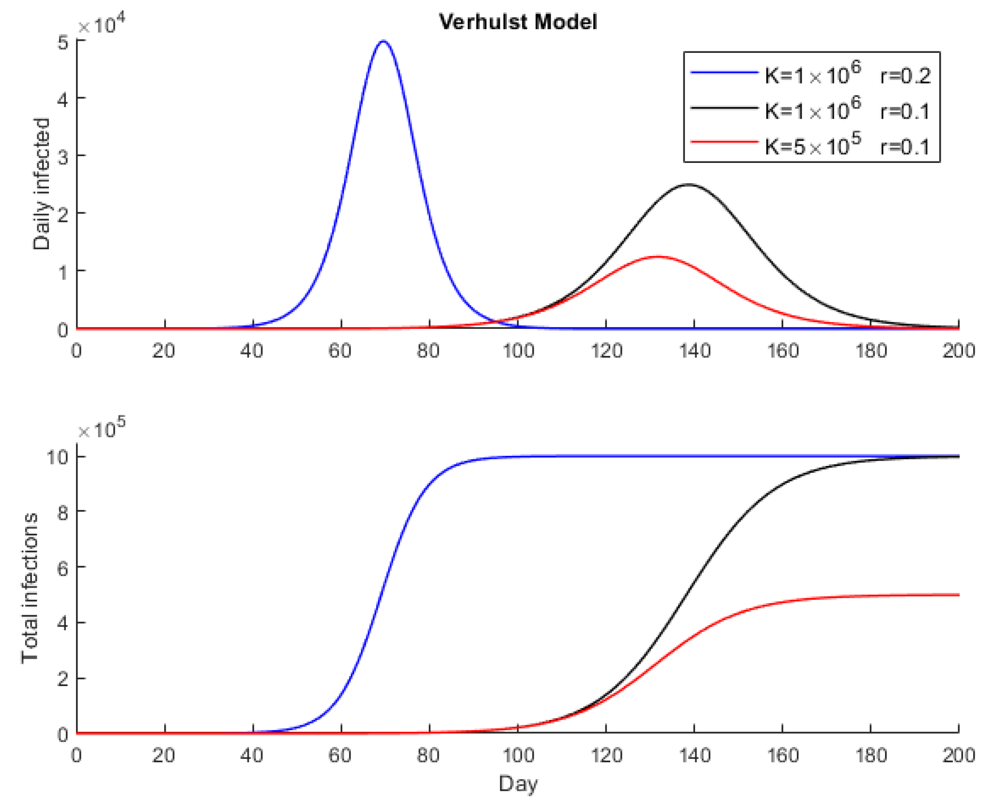
Identical considerations to Verhulst’s model can be made for the peak and the time at which the peak occurs. The number of infected is higher than in the case of Verhulst’s model for the same values of
and
. This result can be seen in
Figure 1 and
Figure 2, in which Verhulst’s and Gompertz’s models were simulated for an initial population
and taking different values of
and
(the same in each model).
In Verhulst’s and Gompertz’s models, the model parameters
and
to
are related via a logarithmic expression. In the case of Verhulst, the logarithmic equation is
In the case of Gompertz’s model, from Equation (8), we obtain
which can be used to obtain a first approximation of
and
by linear regression.
Another possibility is taking logarithms directly in Equation (9):
and solve it for different values of t and by least squares, considering an initial value of
and obtaining the parameters
and
. Analogously, least squares are used to obtain
, proceeding iteratively until the predicted value
satisfies that
is smaller than a fixed value.
3. The Inverse Problem
The inverse problem can be written in abstract form as: , where represents the predicted time series with the parameters obtained by the corresponding model (Verhults or Gormpertz), are the observed data (infected people) in times , and are the model parameters of the prediction problem. For instance, in the Verhulst model , which are the parameters that we need to identify to perform the ad-future predictions.
The data of our problem is a time series containing the number of total infected on each measurement day, so the inverse problem is to find a set of parameters
such as the prediction error:
is less than a certain tolerance
tol, where
represents the predicted time series with the parameters obtained by the corresponding model.
The main source of noise in data, in this case, is the number of infected people, which sometimes corresponds to two consecutive days instead of the same. This is due to the way that the data were transmitted. Additionally, sometimes the criteria to classify the infections has changed over time, causing some data incongruences. Additionally, COVID-19 cases are usually undercounted. All these facts make it so the model should be a useful approximation of reality (noise included) to optimize decision-making. The fact that the L1 norm is used has some implications for the statistical distribution of the outliers due to its robustness in their presence.
The set of models that fit the data with an error smaller than
tol contains the so-called equivalent models
which can be found in a curvilinear valley or even in different unconnected basins [
26]. In this case of a set of plausible values, uncertainty analysis is necessary to obtain a representative sample of the solutions, which will be carried out by a method capable of exploring the set of equivalent parameters to obtain the most plausible one. This method is a member of the PSO (Particle Swarm Optimization) family called RR-PSO (Regressive-Regressive Particle Swarm Optimization), designed by Fernandez-Martinez and Garcia Gonzalo [
27]. It is important to note in this case that casting the inverse problem as a sampling problem makes the use of regularization unnecessary. The only prior information that is used is the search space where the model parameters are sampled. The use of the Metropolis–Hastings (MH) algorithm corresponds to a Bayesian formulation of the inverse problem, while the sampling of the parameters through an exploratory global algorithm, such as RR-PSO, is only a numerical approximation of the posterior distribution of the model parameters provided by a correct theoretical sampler, like MH.
4. Results
The data were obtained from reports provided by the Centro de Coordinacion de Alertas y Emergencias Sanitarias del Ministerio de Sanidad del Gobierno de España [
28].
After obtaining the data on total infections and computing the daily infections, the next step of our study was to set the start and end dates of each wave. As can be seen in
Figure 3, the first wave was the smallest, but in reality, it is believed that there were quite a few more infections than reported by health authorities.
For the purpose of this article, we will focus our attention on the third wave, which starts around 8th December 2020 and is characterized by an upturn in the daily cases a few days after the Christmas holidays (see [
23] for more information).
4.1. Results Comparison
First, using the Verhulst model, really good results have been obtained, which can be found in
Figure 4, where the red dashed line is the observed data and the green one is the best model obtained by minimizing the error. The error obtained was 1.76% with an initial infected population of approximately P0 ≈ 3 × 10⁴, a carrying capacity K ≈ 1.55 × 10⁶, and a growth rate r = 0.086.
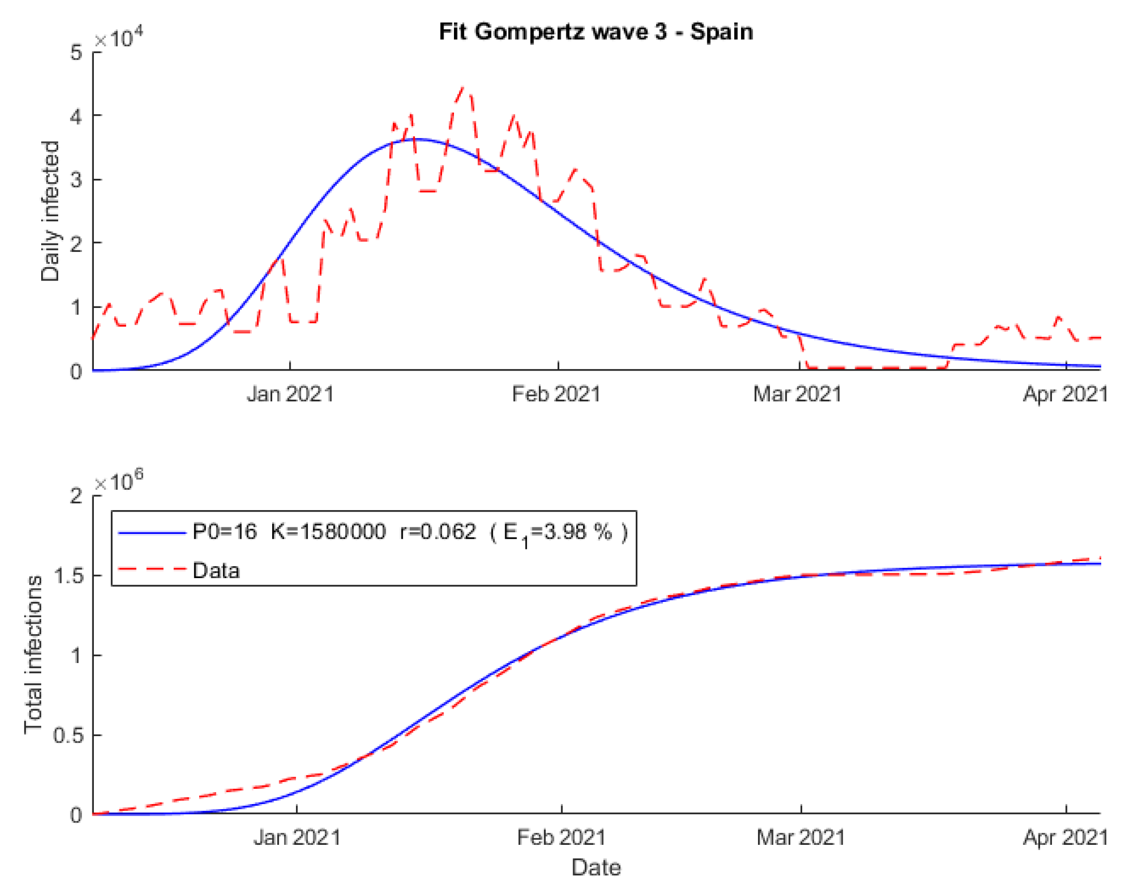
Second,
Figure 5 shows how the fit obtained using Gompertz’s model failed primarily at the beginning of the outbreak, with an error of 3.98%. Furthermore, the initial population obtained, P0 = 16, has been much different with respect to the Verhulst results, and the growth rate is slightly lower, r = 0.062.
Finally, the SIR model returns a precise fit, which can be seen in
Figure 6, with an error of 2.15%, a growth rate of r = 0.255 and a recovery rate of 0.161. It is important to note that, unlike Verhulst’s and Gompertz’s fits, the SIR model does not need to reach the carrying capacity, K ≈ 2.5 × 10⁶, at the end of an outbreak. This could be visualized in
Figure 7, where the epidemic ends because of a reduction in the number of infected people and not due to the lack of susceptibility.
4.2. Predictions
In order to make predictions, it is first necessary to obtain a representative sample of equivalent models. In this paper, the Metropolis–Hastings algorithm, which is a Markov chain Monte Carlo (MCMC) method, was chosen.
After sampling, the next step is to extrapolate the pandemic curves and calculate the different percentiles. The p-percentile of a prediction on one day is the number of infected people left by the p% of predictions below.
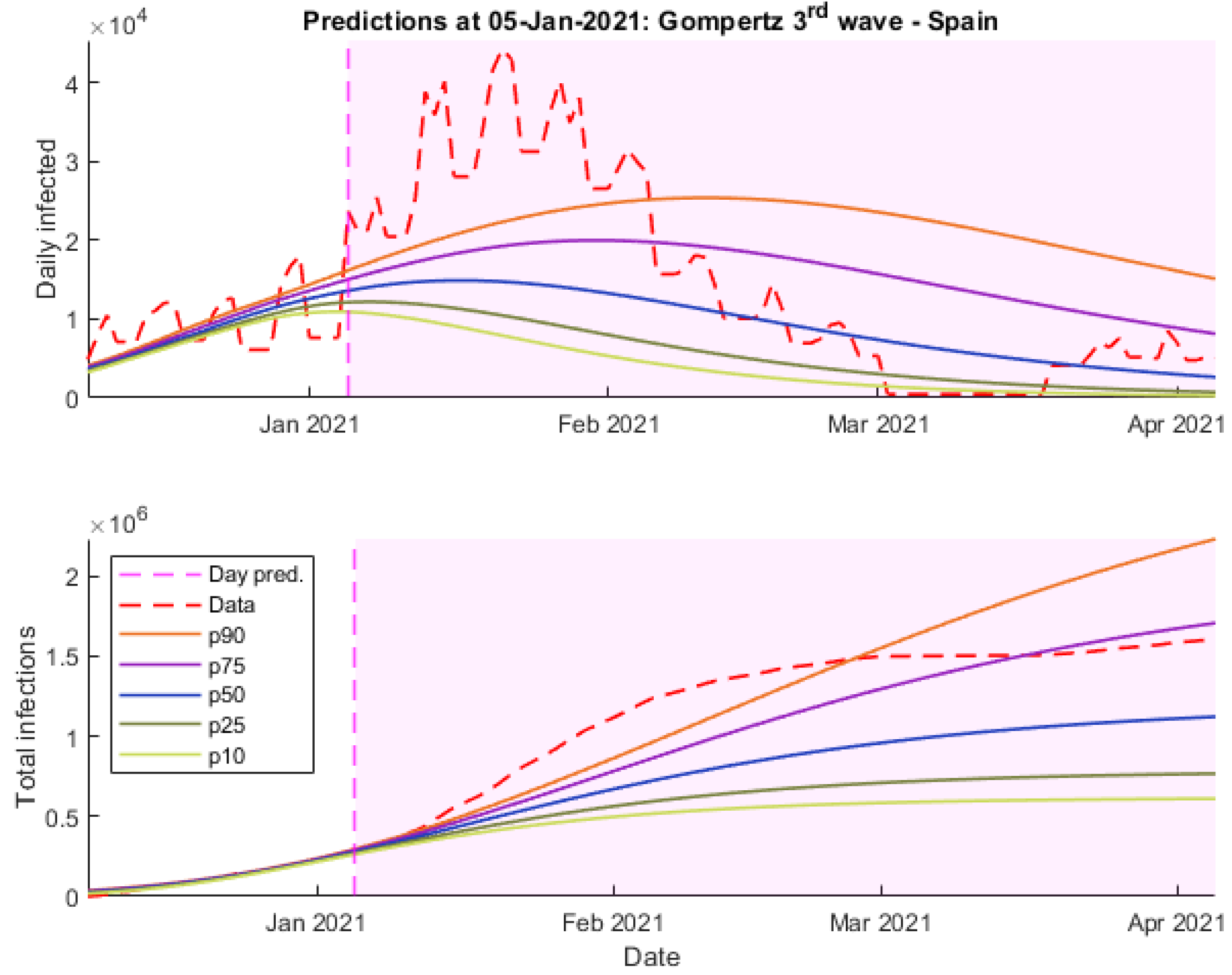
With the aim of giving a general idea about the effectiveness of the different models at making predictions, two examples of it will be presented, the first one made on 5 January 2021 and the second one on 25 January, a few days after the peak of the wave in daily cases.
On the one hand, as it may be seen in
Figure 8,
Figure 9 and
Figure 10, the 75th and 90th Verhulst percentiles are the only ones that correctly predict the fast growth of daily infections at the beginning of the outbreak.
On the other hand, they fail at predicting the end of the outbreak, whereas other models like SIR obtain more accurate predictions. In this case, Gompertz’s model seems like it has not been able to detect the tendency properly due to the lack of data.
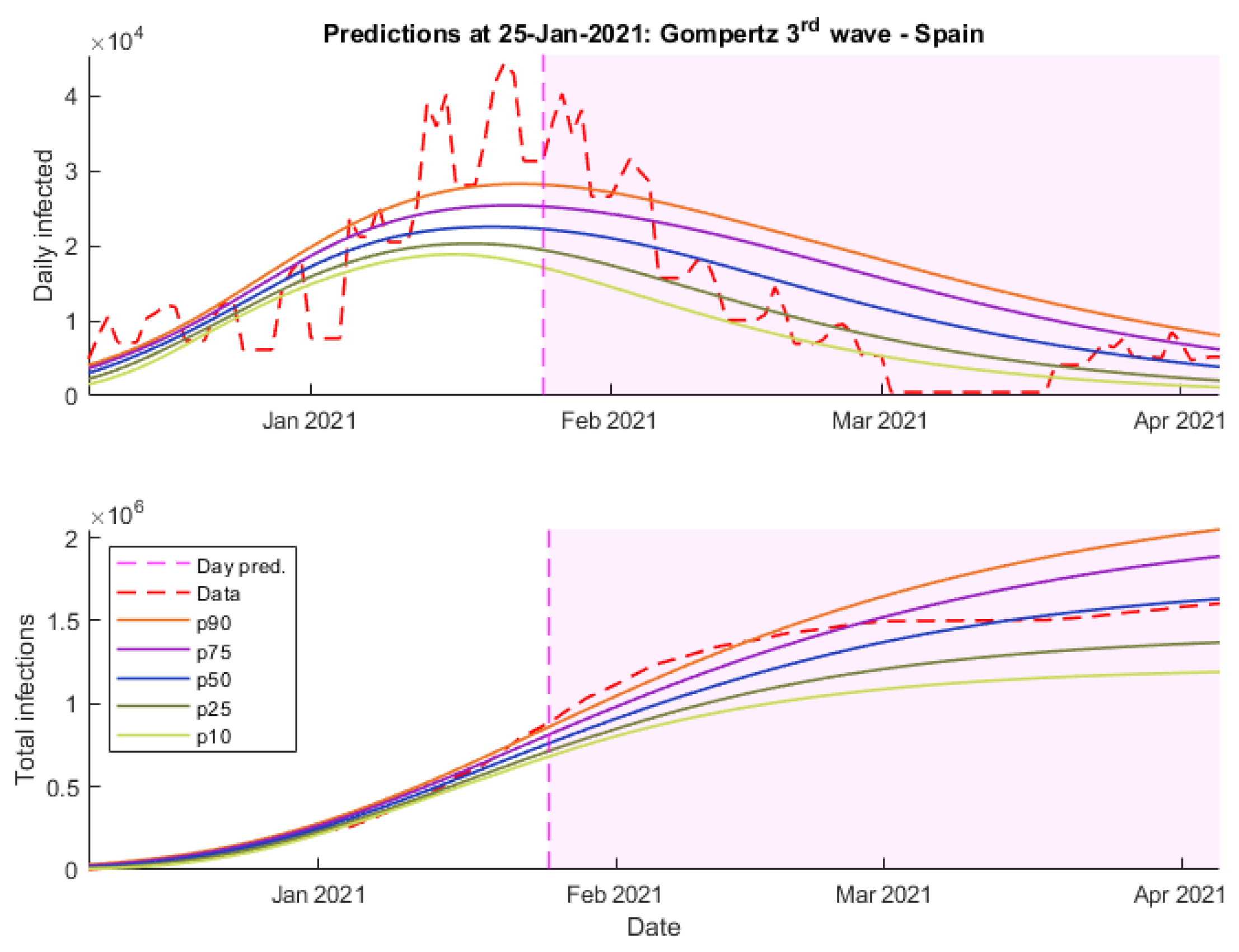
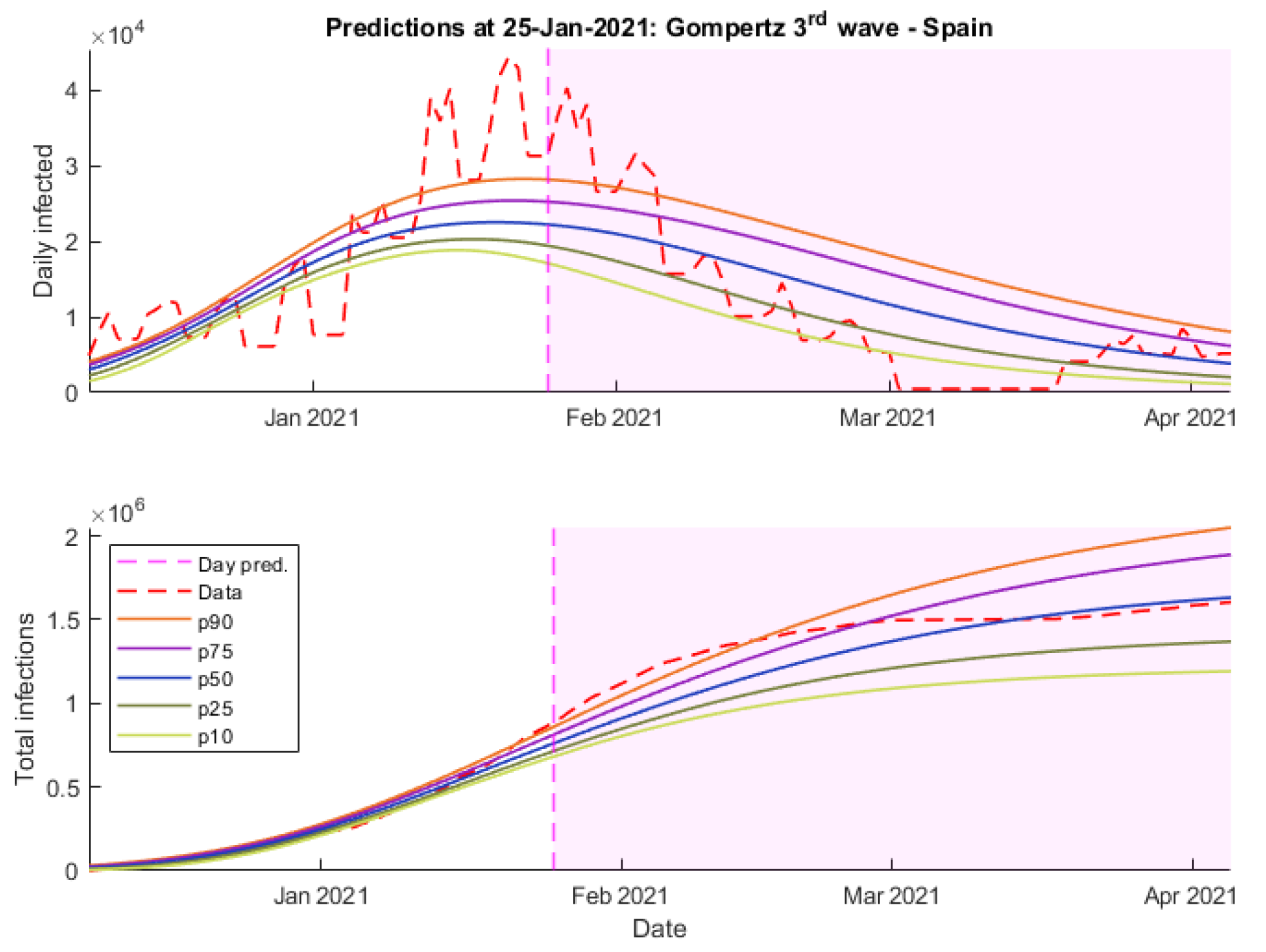
Continuing with the predictions made on 25 January, it can be seen how all the models considerably improved their results.
Figure 11,
Figure 12 and
Figure 13 show the predictions of these three models. For instance, the Verhulst and SIR models (
Figure 11 and
Figure 13) not only allow us to obtain a more precise frame of daily cases, but they fit the wave shape much better.
Finally, as can be seen in
Figure 12, Gompertz’s predictions maintain that long-term trend that fails to adjust the peak of the wave but is the most accurate when it comes to predicting the number of daily cases over April.
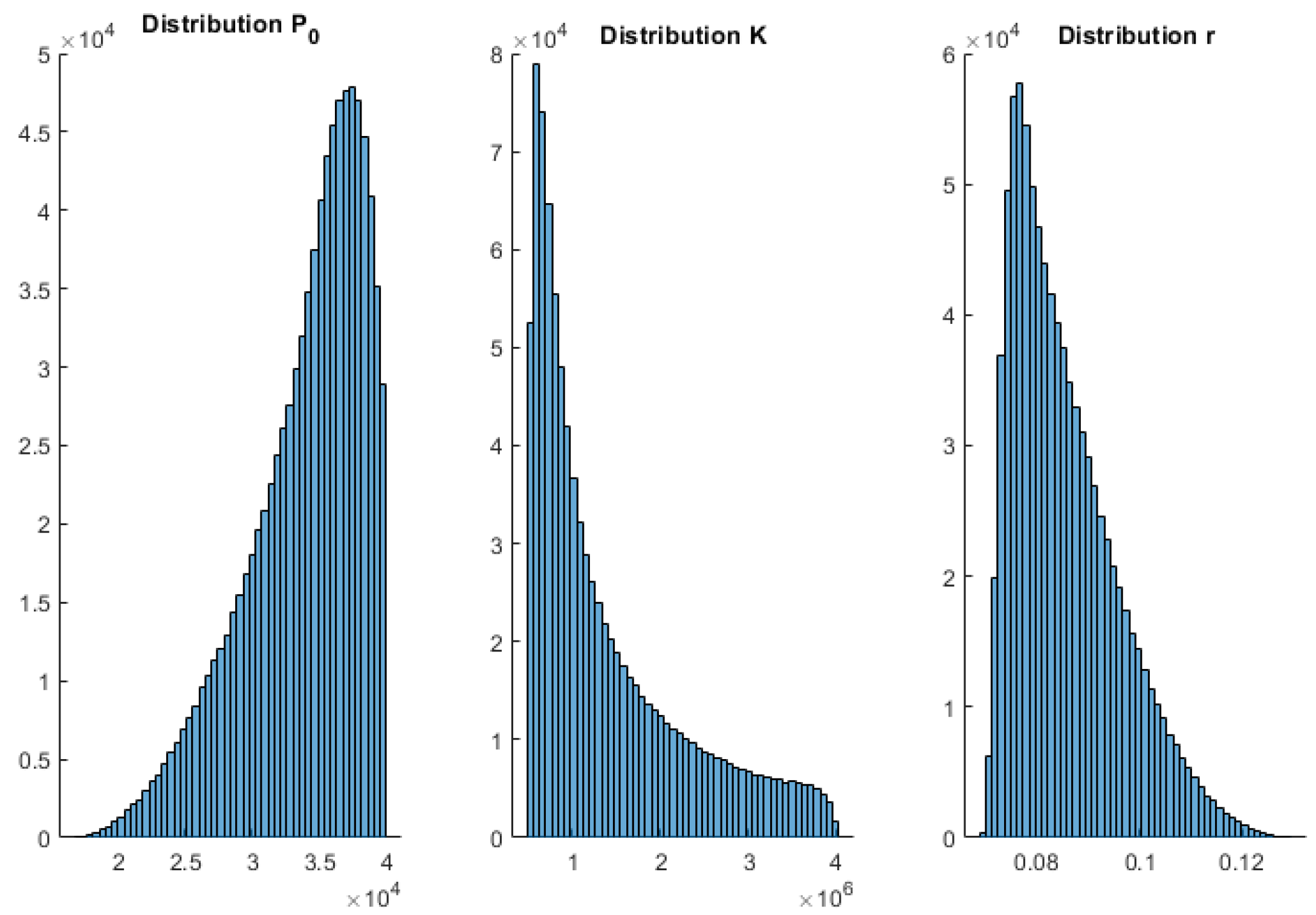
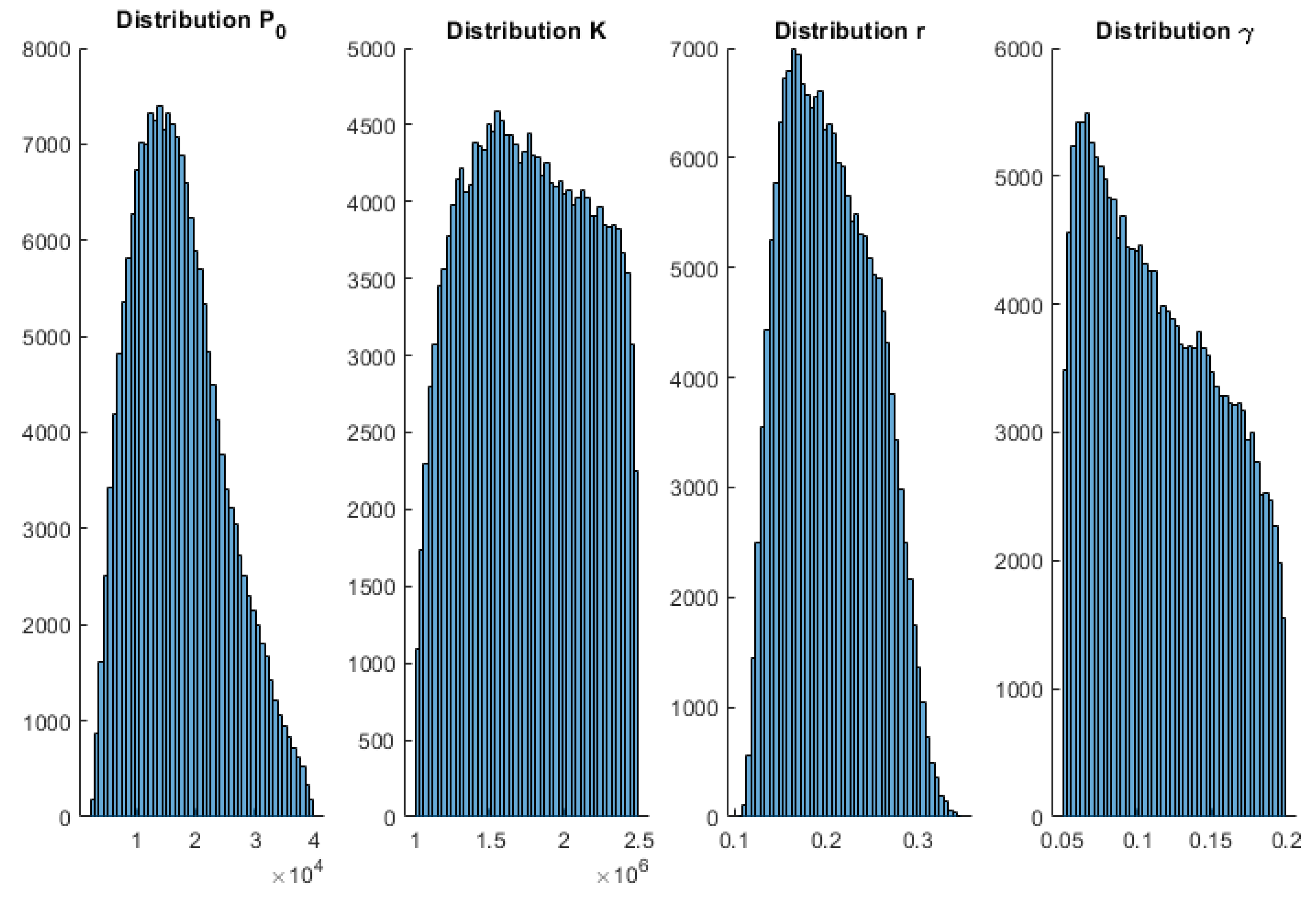
To complement these results,
Appendix A shows the posterior histograms of the model parameters for each of the models and COVID-19 waves. These histograms account for the uncertainty analysis (model appraisal) of the inverse unknowns: initial population, growth rate, maximum population infected (in the case of Verhults’s and Gompertz’s models), and for the SIR parameters via the Metropolis–Hastings algorithm. As can be observed, all the models provide very consistent results. Therefore, the conclusions achieved by the posterior analysis are similar.
5. Conclusions
In this article, a comparison is made between Verhulst’s, Gompertz’s, and SIR models in terms of their effectiveness in predicting the effects of COVID-19 outbreaks in Spain and for the purpose of socio-health planning. The analysis of the different solutions obtained by each model shows the daily prediction of infected people and the total number of infections. All this translates into reliable present and future predictions that are key in determining health measures aimed at the population to mitigate the most serious effects of the next wave.
We show different predictions for COVID-19 in Spain made by each of the models, where the infection rate is between 3% and 10%, i.e., the virus infects between 3 and 10 people out of 100 vulnerable people. The three models show similar results, but it is easier to refine the parameters of Verhulst’s model. In view of these facts, it would be more appropriate to use the Verhulst model for long-term forecasts and the SIR model for short-term forecasts or when precise information on the recovery rate is available. Finally, it is clear throughout the article that none of the models is perfect, but precisely because of these differences in the predictions of each model, they could be used in a complementary way to inform decision-making during a pandemic.


 ,
, 


