1. Introduction
Due to the limitations of geological conditions and exploration techniques, complete and regular geological data cannot be obtained in geological exploration, and sparse data modeling leads to great uncertainty. The method of interpreting and constructing three-dimensional models of complex ore bodies by artificial experience and human–computer interaction is inefficient, arbitrary, and subjective, and makes it difficult to update geological models. To solve this problem, scientists have proposed various geological modeling methods. These are mainly divided into explicit modeling and implicit modeling [
1,
2]. Explicit modeling requires a lot of manpower, time, and effort for complex geological models, and there are many problems such as open mouths and self-intersection. However, implicit modeling does not require a lot of manual interaction, the degree of modeling automation is high, and the local update speed of the model is fast, so it has attracted widespread attention from people in the field of three-dimensional geological modeling.
In the past twenty years, various implicit function interpolation methods have been developed, including deterministic implicit modeling methods (the discrete smooth interpolation method [
3], the RBF method based on radial basis function [
4,
5], the Hermite RBF method [
6], etc.) and stochastic implicit modeling methods (multi-point geostatistical methods). Deterministic implicit modeling methods provide insufficient description of the randomness and uncertainty characteristics of the spatial distribution of geological blocks and geological zone boundaries [
7]. However, multi-point geostatistical random modeling uses borehole data as hard data and training images as soft constraints to reconstruct geological models through multi-point simulation. Geological rules are usually quantified in the training image, which helps us reproduce refined geological models.
Guardiano and Srivastava first proposed using training-image-scanning data templates in 1993 and proposed the MPS method [
8] by replacing the multi-point statistical probability of data events with the probability of different data events. Since then, after more than 20 years of development, scholars have proposed a series of improved strategies and new algorithms [
9,
10,
11] based on this. However, no matter the kind of MPS algorithm, the difficulty in application lies in obtaining training images [
12,
13]. Especially when performing three-dimensional reconstruction, reliable and accurate 3D training images are extremely difficult to obtain, which makes MPS methods difficult to apply effectively in practical three-dimensional modeling [
14].
To improve the applicability of MPS methods, relevant scholars have proposed directly using 2D images (cross sections, plane maps, outcrops, remote sensing images, etc.) to construct training image sequences (training image sequences refer to training image libraries composed of several 2D images) [
15,
16,
17]. Hajizadeh et al. proposed an MPS random modeling method based on the SNESIM (single normal equation simulation) algorithm framework to reconstruct the three-dimensional pore structure of unstructured porous media using 2D training image sequences [
18]. Based on the DS (Direct Sampling) algorithm framework, Comunian et al. proposed the s2Dcd method for MPS simulation. This method uses two or three orthogonal two-dimensional cross sections to construct a training image sequence and fills the entire three-dimensional modeling space by performing a series of two-dimensional simulations [
19]. Chen et al. proposed the 3DRCS method for MPS simulation. The core idea is to use the spatial staggered relationship of a large number of geological sections and plane maps to construct a training image sequence and fill the three-dimensional space through two-dimensional simulation [
20]. Valentin et al. proposed the DeeSse method for MPS simulation. This method obtains a three-dimensional model by superimposing two-dimensional terrain simulation [
21]. Yan et al. proposed the “cross grid, gradual refinement” method to complete the three-dimensional reconstruction of reservoirs using 2D digital images taken by drones [
22].
The above MPS methods based on 2D sequential diagram partition simulation will lead to poor accuracy of simulation results if too few 2D planes are provided. If too many 2D planes are provided, the three-dimensional modeling space is divided into too many partition blocks. It is difficult to capture multi-point statistical information from such limited reference patterns. At the same time, most of the previous MPS methods based on 2D sequential diagram partition simulation adopt an SNESIM algorithm or a Direct Sampling (DS) algorithm improved based on the SNESIM algorithm. The SNESIM algorithm has achieved remarkable results in the stochastic modeling of reservoirs with categorical variables, such as ore body lithology modeling and reservoir sedimentary microphase modeling. However, the method has the following drawbacks: ① When there are too many attribute categories, the modeling effect of the method is relatively poor. Experiments show that when the number of categorical variables is greater than 3, the modeling results of this method begin to deteriorate. ② The SNESIM algorithm is unable to construct a three-dimensional model of continuous variables. ③ When the training image is more complex or the simulation mesh is finer, the method needs to consume a large amount of memory, so usually, for millimeter-level refinement of ore body 3D modeling, the method is difficult to achieve.
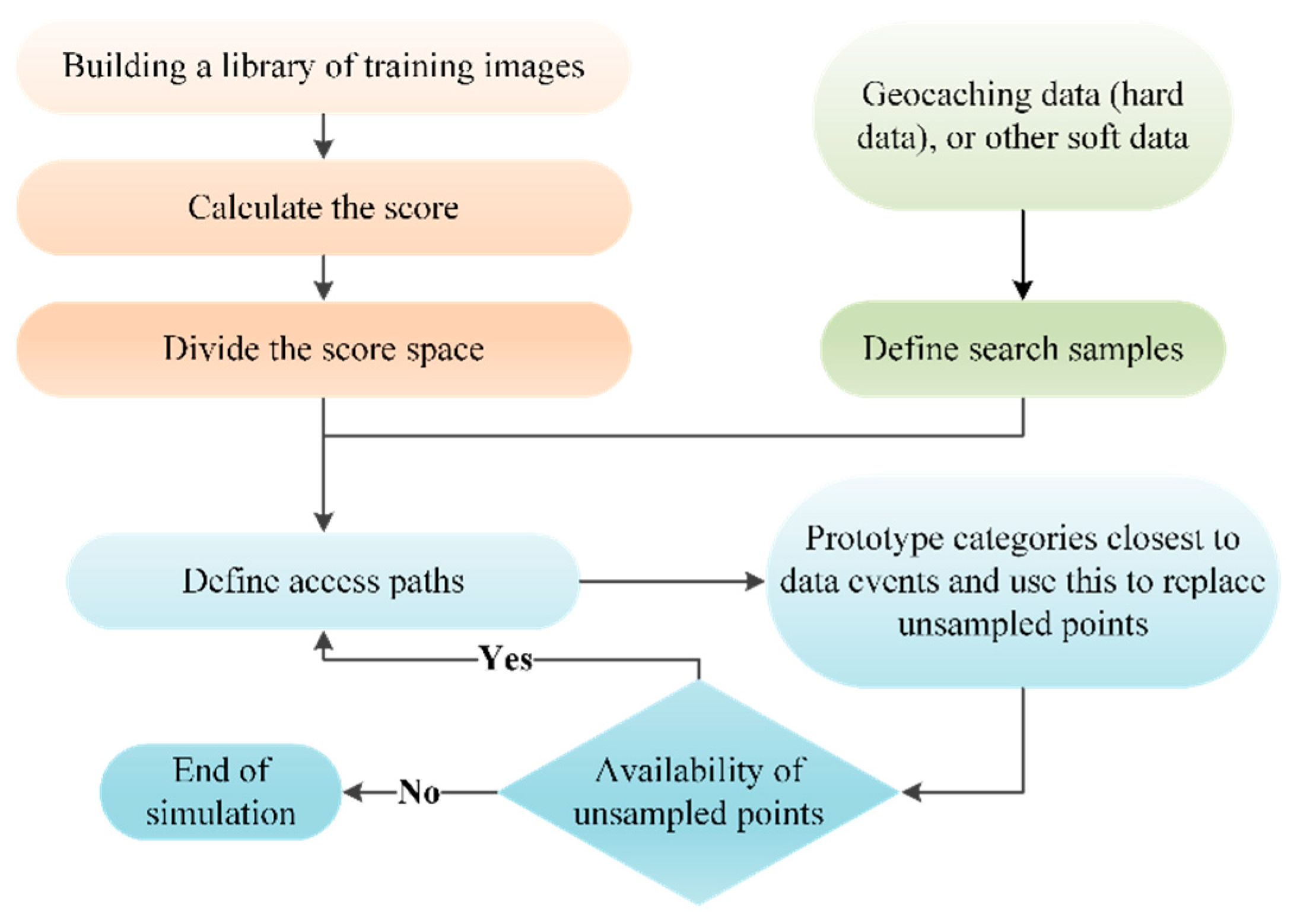
The FILTERSIM algorithm is a good solution to the above problems; it can not only simulate the categorical variables and continuous variables, but can also complete three-dimensional modeling of the ore body under reasonable memory requirements. The algorithm introduces a filter model to reduce the dimensionality of the data, and improves the search speed through clustering analysis, which significantly improves the computational efficiency. The FILTERSIM algorithm is mainly divided into three steps: filter score calculation, pattern classification, and pattern simulation. The flowchart is shown in
Figure 1, and the algorithm implementation steps are as follows:
① Define the data sample specification, scan the training image, and use the filter to calculate the score of each training pattern.
② Classify the training patterns according to the scores and save the score value of each training image.
③ Select the simulation starting point and define the simulation path.
④ Calculate the scores of the data samples, find the training patterns with the most similar scores, and use them to replace the attributes of the unsampled points.
⑤ Repeat the above process until all the unsampled points are simulated.
When reconstructing a three-dimensional copper ore model, Takafuji et al. compared the performance of SNESIM algorithm and FILTERSIM (Filter-based simulation) algorithm. The results showed that the FILTERSIM algorithm simulation results showed better spatial continuity, and it was more representative than the SNESIM algorithm simulation results [
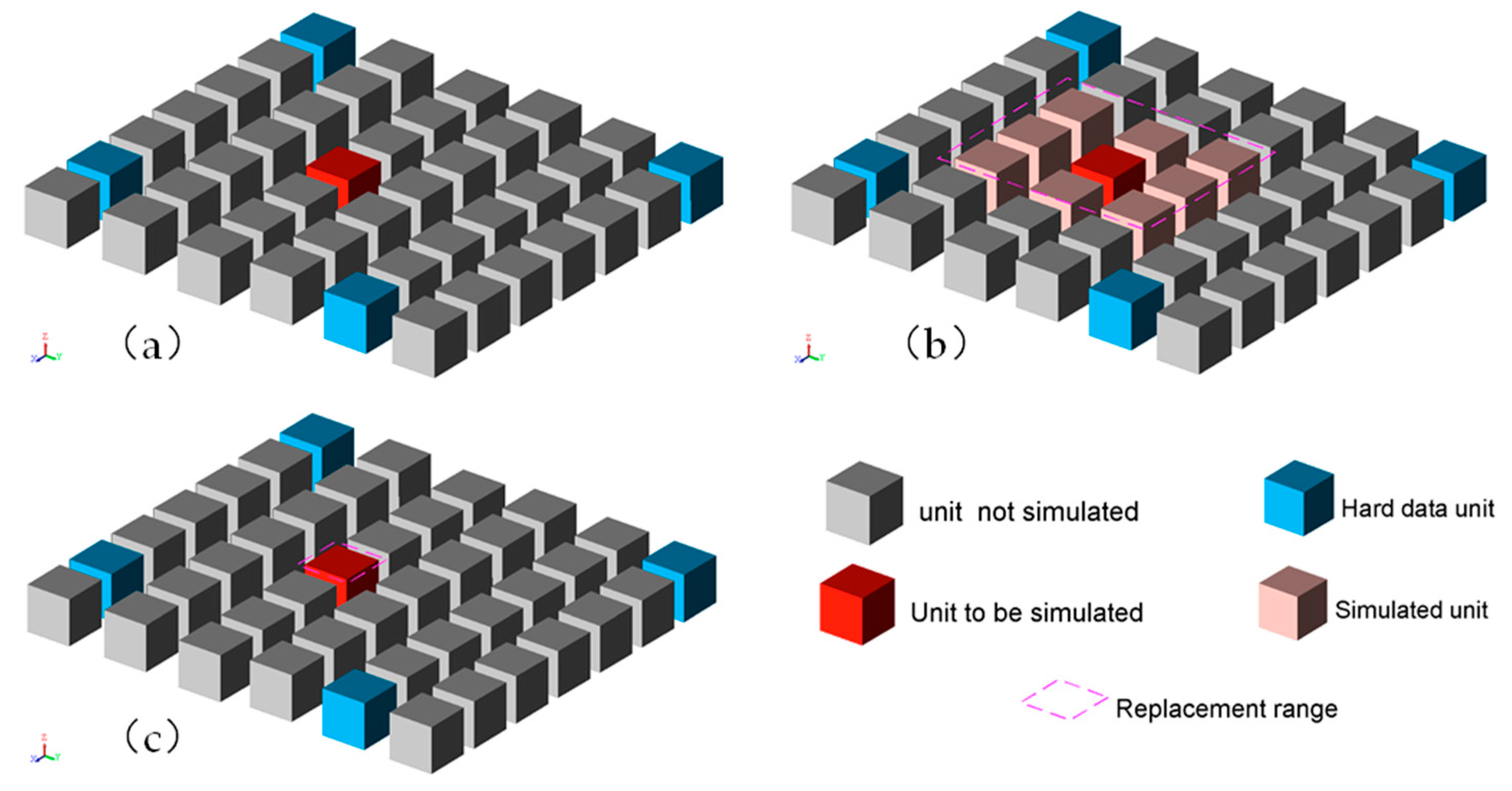
23]. Because the FILTERSIM algorithm replaces the simulated grid with the most similar training pattern as a whole or locally, it ensures continuity of the simulation results. The SNESIM algorithm and a series of algorithms (such as the DS algorithm) derived from its improvement only simulate one Cartesian grid each time, which makes the simulation results too discrete and random, as shown in
Figure 2. In summary, when reconstructing a refined three-dimensional model based on 2D sequential diagrams, two key tasks need to be performed: (1) Construct a reasonable 2D training image sequence. (2) Select a suitable MPS simulation algorithm according to the simulation object.
In order to solve the problem of 2D training image sequences being difficult to construct, an MPS method based on variogram partition simulation is proposed based on the FILTERSIM algorithm framework. In order to ensure the accuracy of the simulation results, this paper defines a new filter and allows the training pattern (the training pattern refers to the grid image extracted from the training image) to be reduced from multiple directions. For the multiple locally similar training patterns (local solutions) generated by the partition simulation, this paper uses information entropy theory to select the training pattern (optimal solution) most similar to the conditional data (conditional data refers to the grid nodes constructed from borehole data) from several local solutions. In addition, in order to construct a refined geological model, this paper uses multiple grids to reconstruct the three-dimensional geological model. Finally, the differences between the new method and the traditional MPS method in simulation accuracy are compared. The results show that the new method has higher simulation accuracy.
2. Two-Dimensional Training Image Plane Partition Simulation Algorithm
The core idea of the MPS modeling method based on 2D training image partition simulation is as follows: firstly, divide the simulation partitions with variogram values, and then, construct 2D training image sequences based on this; then, embed the partition strategy into the FILTERSIM algorithm framework; finally, add new filtering strategies and information entropy theory in this framework to reconstruct accurate and reliable three-dimensional geological models. For a complete overview of the FILTERSIM algorithm, please refer to Zhang et al. [
24,
25].
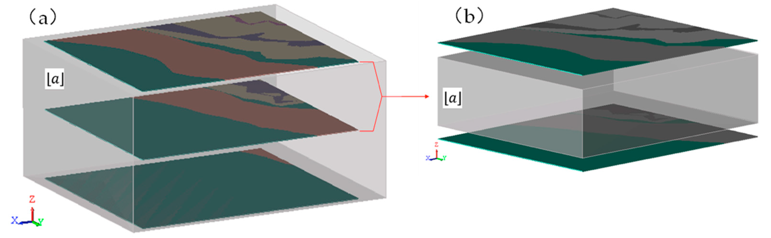
Figure 3 shows a schematic diagram of 2D training image sequence partition simulation. The variogram of geological attributes in the N-S direction is
. Plane maps are drawn along the vertical direction with
as the spacing to construct the training image sequence. The three-dimensional modeling space is divided into two subspaces by three planes in the N-S direction, and each subspace is surrounded by two training images (
Figure 3a). For any unsampled point in the local subspace, MPS simulation only obtains data from the two training images surrounding the subspace, not the entire training image sequence (
Figure 3b). In other words, there are two training images available for scanning at each simulation position. The variogram can reflect the spatial anisotropy of geological attributes, so it is more reasonable and credible to divide the simulation space with the variogram.
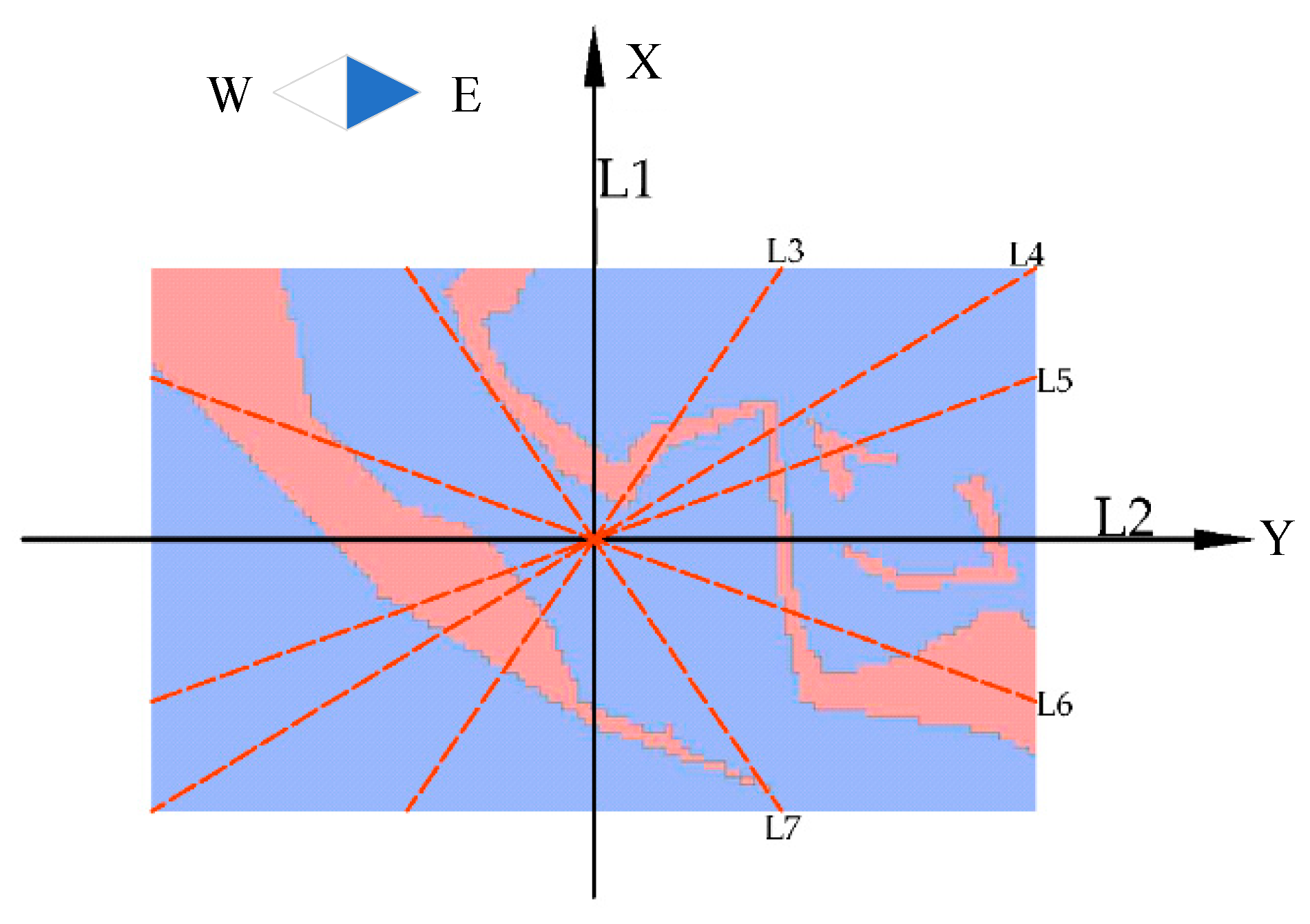
The FILTERSIM algorithm provides three linear filters to reduce the dimension of the training pattern, which can represent a 2D or 3D image as a weight (or score), that is, only the center position of each training pattern is stored in the memory, which reduces the demand for computer memory in MPS simulation and improves modeling efficiency. The FILTERSIM algorithm filters the filtering score to distinguish the dissimilarity of the training patterns, so fast and accurate calculation of the filtering score of the training patterns is the key step in MPS simulation. The new method adds a covariance filter based on the original filters. In addition, the FILTERSIM algorithm only reduces the dimension of the image in the
direction and the
direction, such as L1 and L2 in
Figure 4. Zhang et al. pointed out that it is difficult to accurately reduce the dimension of nonlinear data from only two directions [
26]. In order to better distinguish the dissimilarity of training patterns, the new method allows the filter to filter the training patterns from multiple directions, such as L3, L4, L5, L6, and L7 in
Figure 4. The advantage of this strategy is that it can better capture the diversified characteristics of the training pattern.
Partition simulation needs to scan multiple training images, so it will generate multiple similar training patterns. As shown in
Figure 3b, MPS simulation will extract training patterns (local solutions) similar to the conditional data from the upper and lower training images, respectively. These two local solutions may be similar or may have obvious deviations. There are two solutions to this problem: (1) Compare the scores of the two training patterns and choose the training pattern with the minimum score distance from the conditional data. (2) Determine the preferred method and theory of training patterns according to geological attribute characteristics and user needs (such as information entropy, Kalman filter, etc.). Theoretically, both solutions are feasible, but the latter selects training patterns with better continuity and more representativeness.
2.1. Define Filters and Filtering Directions
The FILTERSIM algorithm can accept two forms of filters: default filters and user-defined filters [
25]. By default, the FILTERSIM algorithm provides three filters for the
direction (the mean Formula (1), gradient Formula (2), and curvature Formula (3)). The filter structure and search template size are the same, where
is the template size in the
direction (
indicates
), and
and
are the offset of the filter nodes in the g direction. They can represent the training pattern as a set of score values
(as shown in Formula (4)), where
is the template center node;
is the simulated node value;
, and
is the template size in a certain direction.
Using the three default filters to reduce the dimension of the training pattern in
Figure 5, and then, analyzing the three sets of scores in the
direction by the factor analysis method, the results show that there is only one main factor in the calculation results of Formulas (1)–(3). Formula (5) defines a new filter (covariance filter) in this paper.
Compared to the other three filters, the covariance filter is more capable of retaining the edge information of an image and is more sensitive to capturing localized features and changes in the image. It is able to better identify local textures, patches, or other features in an image by taking into account the covariance between pixels, so that this information is better preserved in the dimensionality reduction process. Using the above four filters to reduce the dimension of the training pattern in
Figure 5, the factor analysis method calculates the results, as shown in
Figure 6, where filter numbers 1 to 4, respectively, indicate the covariance, mean, gradient, and curvature filters. The scree plot turns at the third feature point, and the feature values of the first two points are both greater than 1, indicating that there are only two main factors in the above four filters.
Section 3.2.1 analyzes the performance of the four filters. The results show that the gradient filter and the covariance filter are superior.
There are limitations in filtering (reducing dimension) 2D or 3D training patterns only from the
direction and
direction in the FILTERSIM algorithm. In order to fully capture the diversified characteristics of the training pattern, the new method allows the filter to reduce the dimension of the training pattern from any direction. In MPS simulation, there are two ways to represent the filtering direction of the filter: (1) Set the tolerance angle (the tolerance angle is the angle between adjacent filtering directions); (2) Specify the specific filtering direction angle value (range from 0° to 180°, as shown in
Figure 4). This paper achieves the dimension reduction of training patterns through the former, and the filtering direction with a tolerance angle of
is
. Obviously, the smaller the tolerance angle, the more filtering directions there will be, and the diversified characteristics of the training pattern can be captured more accurately. However, too small a tolerance angle will consume a large amount of computer memory and modeling time. Therefore, the size of the tolerance angle
should be within a suitable range.
2.2. Weighted Method to Select the Optimal Pattern
The core aim of MPS simulation is to find the training pattern most similar to the conditional data. For the multiple similar training patterns generated by the partition simulation, this paper considers using a nonlinear, objective, and practical method to select the training pattern most similar to the conditional data. Christakos et al. introduced entropy in geostatistics to measure the uncertainty of the probability density function [
27]. Deutsch et al. used information entropy to evaluate the spatial disorder of geological models [
28]. Silva et al. used spatial information entropy to evaluate the spatial disorder of MPS training images [
29]. In fact, the difficulty in calculating information entropy lies in obtaining an accurate probability density function. He et al. used multi-point density function scanning of geological models to obtain probability density functions [
30].
In order to fully reproduce the spatial continuity of the geological model, this paper hopes to select a result that is most similar to the conditional data, has good continuity, and is more representative from two similar training patterns. The new method uses information entropy to calculate the weights of each training pattern, and then, selects the training pattern according to the weight values. The better the continuity of the training pattern, the greater the weight; the worse the continuity, the smaller the weight. The information entropy formula is Formula (6) [
31,
32], where
is a discrete variable of n different probabilities. The weight of the evaluation indicators formula is Formula (7).
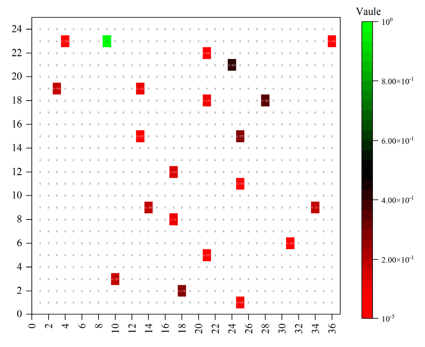
To demonstrate that entropy values can be used as a measure of uncertainty in the probability density function, the following example is given.
Figure 7 shows two similar training patterns with some differences in continuity. We scanned the training patterns with a rectangular template containing two attributes and four positions, and a total of 16 configurations were obtained, as shown in
Figure 7. By calculating the entropy values of the two patterns, it is possible to quantitatively analyze that the uncertainty of pattern A (
HA = 0.92) is higher than that of pattern B (
HB = 0.80). The weight of mode B (
WB = 0.108) is calculated to be higher than that of mode A (
WA = 0.046). Therefore, training mode B was selected as the optimal simulation result.
2.3. Detailed Algorithm Flow of Partition Simulation
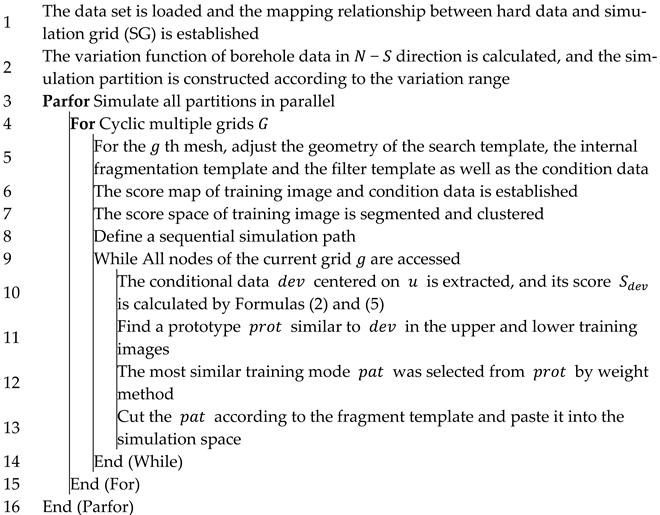
In summary, the detailed algorithm flow of the MPS modeling method based on 2D sequence graph partition simulation is described in Algorithm 1. For each independent partition, this paper uses multi-thread parallel operation to improve modeling efficiency. In order to accurately capture the diversified characteristics of the training patterns, this paper reduces the dimension of the training patterns from multiple directions using Formulas (2) and (5). In order to simulate a stratigraphic model with good continuity and more representativeness, the weighted method is used to select the optimal solution from multiple similar training patterns.
| Algorithm 1: MPS modeling method using 2D training image partition simulation |
![Mathematics 11 04900 i001]() |
4. Comprehensive Example—3D Strata Reconstruction
For the Xishan Yao Formation of a uranium deposit in Xinjiang, China, the new method proposed in this paper is used for modeling and compared with the results of other methods. The study area is the sand body of the lower section of the Xishan Yao Formation, a sand body with a high degree of control in the survey area, with a length of more than 1200 m and a width of 1300 to 2500 m. The net thickness of the sand body ranges from 7.60 to 40.75 m, with an average of 27.64 m, and a coefficient of variation of 23.57%, and the morphology of the sand body is simple, with a continuous distribution on the planar surface. The sand body is thick in the south-east and gradually thins toward the north-west. The internal structure of the sand body is the most complicated among all the ore-bearing sand bodies. On the whole, the thickness of the mudstone interlayer in the ore-bearing sand body in the detailed investigation area gradually increases from the south-east to the north-west, and generally, the ore-bearing sand body is interspersed with 1–3 layers of mud interlayer, with a thickness of 0.20–16.20 m and an average of 3.08 m, and the length of the mud interlayer in the profile varies from 50 to 400 m. Most of the sand bodies show the following coarse upper layer, with a thickness of 40.75 m, and a variation coefficient of 23.57%. Most of the sand bodies are characterized by a sedimentary pattern of coarse at the bottom and fine at the top, with some sections forming a coarse–fine–coarse pattern. The study area is the C16 mining area of the uranium deposit. There are 95 boreholes in this area, and the borehole data are shown in
Figure 8.
Section 3.1 calculates that the range of borehole data in the direction is about 10 m.
Figure 15 shows 12 training images obtained from borehole interpretation.
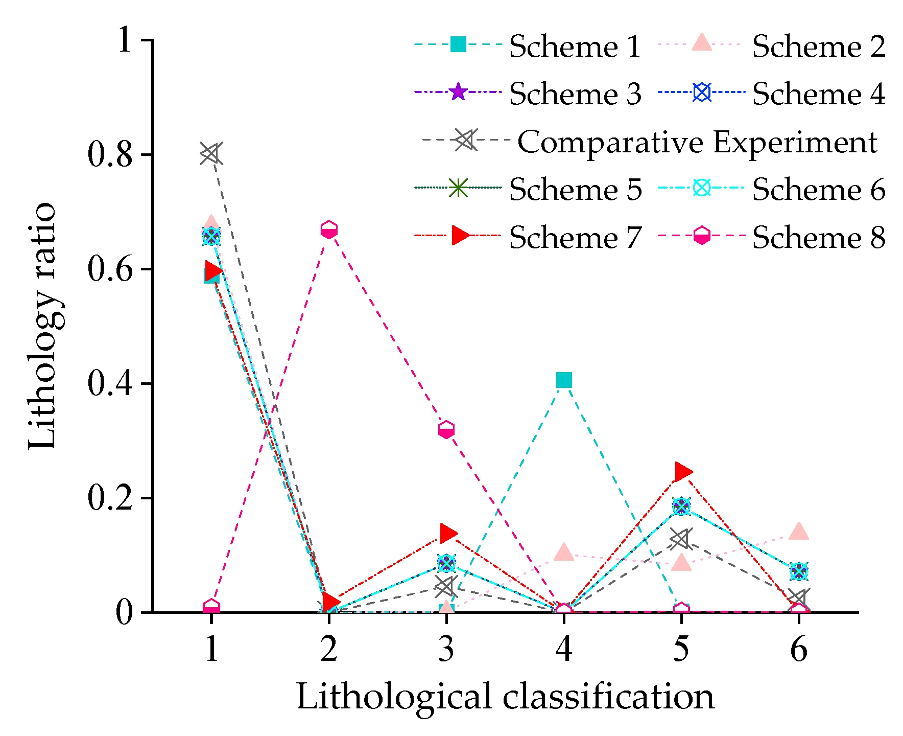
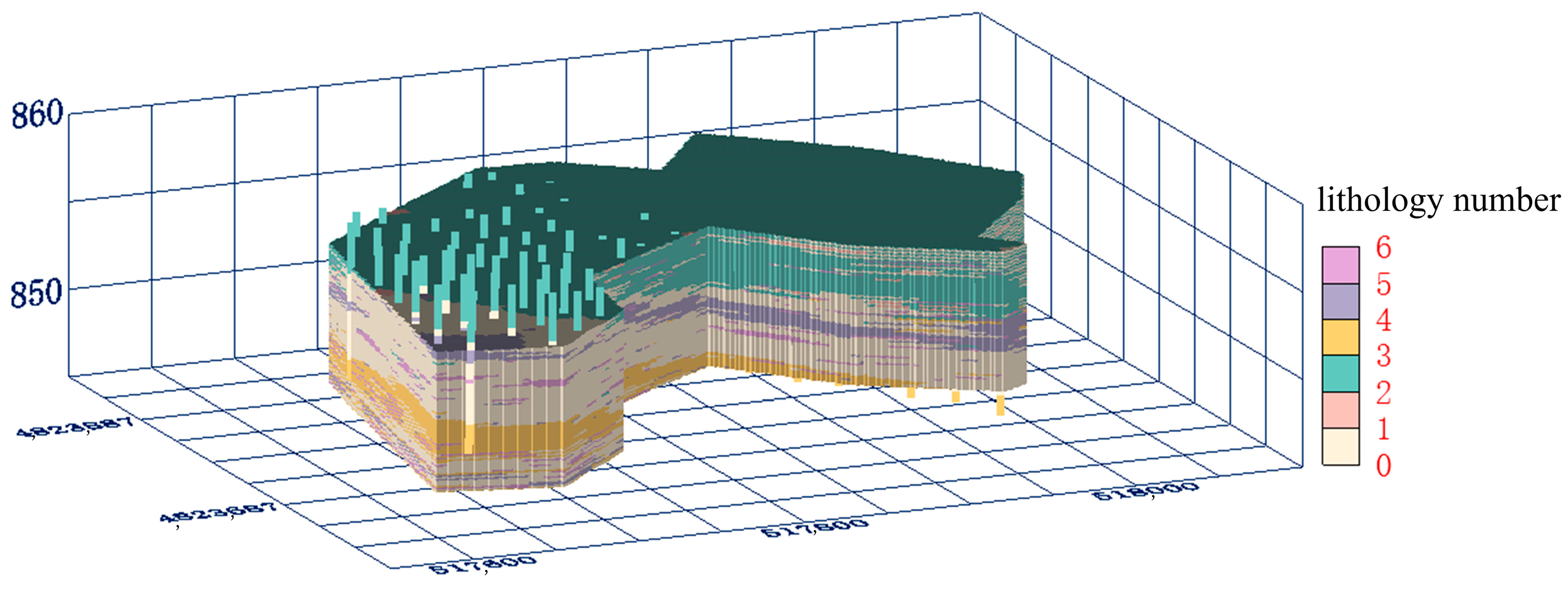
Table 3 shows the basic parameters of a single training image. There are six lithologies in the modeling area: sandstone, the coal seam, the top plate, the bottom plate, mudstone, and a sandstone–mudstone mixture, which are represented by numbers 1 to 6, respectively.
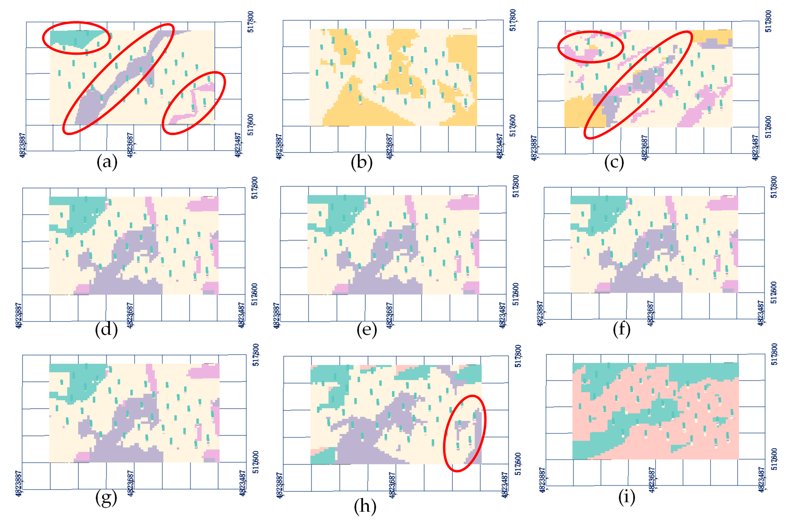
For the training images shown in
Figure 15, this paper studies the modeling ability of three different MPS methods: the new method (partition simulation FILTERSIM algorithm), the traditional FILTERSIM algorithm, and the SNESIM algorithm. In order to compare the accuracy of the simulation results of the three methods, five boreholes are left out of the borehole database shown in
Figure 8 and are not involved in strata modeling. The simulation results of the three methods are compared with the five reserved boreholes, respectively. In this way (“borehole sampling detection”), the ability of the three methods to reconstruct complex three-dimensional strata is compared.
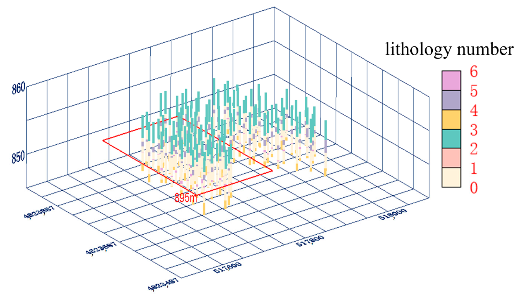
Figure 16 shows the three-dimensional strata model of Tianshan uranium mine simulated by the new method.
Figure 17 and
Figure 18 show the borehole detection results of the simulation results of the three MPS methods. Obviously, the new method has the highest accuracy in simulating strata models, the accuracy of the five boreholes is greater than 80%, and the average value of accuracy is 86.21%; the traditional FILTERSIM algorithm simulates the rock model with the second highest accuracy with an average value of accuracy of 74.85%, and the new method improves the accuracy of the simulation results by 11.36% compared with the traditional MPS method. In addition, it can also be found that the accuracy of the FILTERSIM algorithm simulation results is significantly higher than that of the SNESIM algorithm. This shows that the FILTERSIM algorithm simulation results are more representative, which is the same as the research conclusions of Takafuji et al. [
23]. The new method has two typical characteristics: (1) The MPS simulation results are captured from two training images surrounding the subregions. (2) The filtering algorithm in this paper can accurately determine the similarity between training patterns and conditional data. These features ensure the ability of the new method to reconstruct complex 3D strata.
5. Conclusions
This paper proposes an MPS method based on variogram partitioning to reconstruct three-dimensional models. For a long time, the difficulty in applying MPS methods has lain in constructing accurate and reasonable training image sequences. Especially when using 2D graphics for three-dimensional reconstruction, the position and number of 2D training images will directly affect the simulation results. The new method uses a variogram to construct simulation partitions, and then, formulates a training image sequence based on the partitions. The variogram partitioning strategy ensures the reliability of the training image sequence. At the same time, a series of sensitivity and performance analysis experiments have verified the applicability and accuracy of the new method in 3D strata simulation.
Compared with existing multi-point geological statistical reconstruction methods based on incomplete data sets (2D images), the new method has two advantages: First, the idea of variogram partitioning eliminates the influence of the number of training images on the simulation results; second, the simulated results have good continuity and more representative strata models. In the field of MPS geological modeling, many scholars believe that FILTERSINM algorithm simulation results are superior to those of algorithms such as SNESIM. Therefore, this paper embeds the partitioning strategy into the FILTERSIM algorithm framework. At the same time, in order to ensure the reliability and accuracy of the new method’s simulation results, this paper proposes a series of innovative methods.
The core of the FILTERSIM algorithm is to reduce the dimension of 2D or 3D training patterns. Compared with the existing FILTERSIM methods, this paper proposes new filters that can fully capture the diversified characteristics of training patterns, and allow training patterns to be reduced from multiple directions. The performance analysis of four filters proves that the gradient filter and covariance filter are much better than the mean filter and curvature filter in reducing the dimension of training patterns. The results of the tolerance angle sensitivity analysis show that increasing the filtering direction can improve the dimension reduction ability of the filter. For multiple similar training patterns generated by partition simulation, this paper uses information entropy to select the optimal simulation results.
In order to verify the accuracy of the new method, this paper applies the new method in a real geological example, and compares the new method with two existing MPS methods (the FILTERSIM algorithm and SNESIM algorithm). The borehole sampling detection experiment results show that the new method has the highest accuracy in simulation results. These experimental analyses show the superiority of the new method in all aspects.


