Abstract
In this study, the authors verify fixed-point results for Geraghty contractions with a restricted co-domain of the auxiliary function in the context of generalized metric structure, namely the -metric space. This new idea of defining Geraghty contraction for self-operators generalizes a large number of previously published, closely related works on the presence and uniqueness of a fixed point in -metric space. Also, the outcomes are achieved by removing the continuity constraint of self-operators. We also provide examples to elaborate on the obtained results and an application to the integral equation to illustrate the significance in the literature.
MSC:
58C30
1. Introduction
The development of other sciences depends heavily on mathematics, and the natural sciences are intimately interconnected. As a result, mathematicians are constantly attempting to create methods and systems that will enable other fields to advance. When it comes to helping mathematicians solve models in partial and ordinary differential equations developed by physicists, engineers, or chemists, one of the most effective tools at their disposal is the fixed-point methodology in metric spaces having a symmetric property. Additionally, the fixed-point theory is still regarded as a vital tool in the advancement of research in numerous fields and disciplines, including dynamical systems (and chaos), functional analysis, economics, logic programming, artificial intelligence, differential equations, topology, and game theory.
It is important to remember that the first mathematical discovery to focus on fixed points (FPs) for mapping under particular kinds of contraction conditions was Banach’s contraction theorem (BCT) [1]. Mathematicians started extending the Banach contraction theorem in a variety of ways because of the significance of fixed points. Some generalized the Banach contraction condition in numerous ways, while others extended metric spaces to new spaces and expanded the Banach contraction theory to new forms. For example, the concept of metric space is generalized to b-metric space [2], S-metric space [3] and these two generalizations of metric space are combined to introduce the concept of -metric space [4,5,6]. Furthermore, in order to provide novel fixed-point results, others have introduced more generic contraction conditions.
Utilizing an auxiliary function with the condition gives . Geraghty [7] introduced the Geraghty contraction, an intriguing contraction condition, in 1973 and illustrated certain FPs under this condition by extending BCT into a complete metric space (CMS). Numerous authors have dedicated a great deal of attention to Geraghty’s results. In metric-like space, Aydi et al. [8] examined FP theorems for a new type of Geraghty contractions, Karapinar et al. [9] expanded the theory in generalized metric structure, namely b-metric-like-space, Wang et al. [10] presented intriguing results pertaining to FP consequences through the notion of Geraghty contraction-type maps in —metric spaces, and very recently, Alam et al. [11] solved a two-point boundary value problem introducing rational-type Geraghty contraction.
Wang et al. [10] obtained the following result by generalizing the result obtained by Karapinar et al. [9].
Theorem 1
([10]). Let T be a mapping defined on X, where is a complete -metric space. Let be such that
for all , where and g satisfies . Then, T has a distinct fixed point .
Following Geraghty [7] and Wang et al. [10], we explored new Geraghty types of contractions in the context of -metric space. The auxiliary function, which is used to define the first contraction, has a restricted co-domain and a limiting condition that is different from the limiting condition of Geraghty. We demonstrate that the self-operators that fulfill this contraction need to have only one fixed point within the framework of -metric spaces. Additionally, examples are provided that explain the obtained outcomes, and a utilization of the integral equation demonstrates how significant they are in the literature. The primary goal of this work includes assisting young researchers by providing a framework for Geraghty-type outcomes in -metric space and demonstrating that there is still an opportunity for many more researchers to explore this intriguing area with its vast potential for applications.
2. Preliminaries
We now look over several definitions, illustrations, and results that are pertinent to understanding this work.
Definition 1
([6]). Suppose X is a nonempty set. Let and . Let be a mapping satisfying the properties listed below:
- (i)
- , for all with ;
- (ii)
- , if and only if ;
- (iii)
- , for all .
Then, the mapping is called an -metric and the pair is called an -metric space for .
Definition 2
([4]). An -metric for is called symmetric if
Lemma 1
([6]). In any -metric space for , we have
Lemma 2
([6]). In any -metric space for , we have
Definition 3
([6]). In an -metric space for , the sequence in X is said to be:
- (i)
- Convergent to the point , if for any given , there exists such that or , for all , and it is denoted by .
- (ii)
- A Cauchy sequence if, for some given , we can find some such that , for each .
Definition 4
([6]). A complete -metric space for is that space in which every Cauchy sequence in X is convergent in X.
Now, we recall the following collections of functions with examples. Let be the set of all those functions g with the condition ⇒ and be the set of all those functions g with the condition ⇒, where .
Example 1.
Let
Then, .
Example 2.
Let
Then, .
3. Main Results
We begin our main outcome with the following theorem.
Theorem 2.
Let A be a self-mapping in a complete -metric space for such that satisfies
for all , where
Then, the mapping A fixes a unique point .
Proof.
Suppose is an element of W. For , let us construct a sequence in W as . For some , if , then we know that is a fixed point of A. In this case, the proof is completed. Thus, let , for all . From (1), we have
where
Take
From (3)
Let such that . Then, by (6), we have
which is a contradiction. Therefore, , for all . From (6), we have
That is, the sequence of real is decreasing. Suppose there exists such that . Let . Letting in (8), we have
Now, we have two cases.
Case II: If , according to (9), we have
which is in conflict.
From the above two cases, we assume , that is,
Utilizing the properties of -metric space, we have
Thus, we obtain
We shall prove the sequence in is a Cauchy sequence; i.e.,
will be proved.
Let us assume (17) is not true, so there exists some for which we can find two subsequences and of with such that
and
By inequalities (18), (19) and Lemma 2, we have
Taking in (20) and using (14), we obtain
From (1), we have
Let and taking in the above equation and using (14) and (19), we obtain
Thus,
From (21) and (24), we have
Hence,
Since , utilizing (14) and (16), we have
From (14) and (27), we have
a contradiction. Thus,
This shows that is a Cauchy sequence in . So, there exists , such that
From Lemma 1 and (30), we obtain
Now, we need to prove that is some fixed point of A. Suppose , then . From (1) and (2), we have
where
We also have
Taking and utilizing (30), (31), and (33), we obtain
Therefore,
Since , then
which is a contradiction. So, and so . Consequently, A fixes the point u.
To prove the distinctness of this fixed point, let be another fixed point of A; that is, and . Now,
and by (1),
which is a contradiction. So, A fixes a unique point. □
The example below illustrates the above result.
Example 3.
Let be endowed with the -metric for , given by
Consider as and . Take
For .
For,
For
Thus, (1) holds for all ; that is, all hypotheses of Theorem 2 are satisfied, so A must fix a unique point. Clearly is such point with .
Next, we prove the following theorem.
Theorem 3.
Let be defined in a complete -metric space for and such that
for all , where
Then, the mapping A fixes a unique point .
Proof.
Suppose is an element of the space W. For , let us construct a sequence in W as . For some , if , then we know that is one of the fixed points of A. In this case, the proof is complete. Thus, let for all . Using (40), we have
where
Take
From (42), we obtain
Let be such that . Then, from (45), we obtain
which is not possible, as . Thus, for all , . So, is a decreasing sequence. Consequently, , for some . Next, we prove that
From (45), we have
Taking in (48), we have
We obtain
Since ,
Therefore,
Thus, we have
From Lemma 1 and (53), we obtain
Next, we want to show that is a Cauchy sequence, i.e., to prove
On the contrary, we assume that (55) is not true. So, there exists some depending on which we can find the subsequences and of with such that
and
By (40) and (56), we obtain
where
Utilizing (58) and (59) in (53), we obtain
On the other hand, using (57), we obtain
Taking , we have
By (60) and (62), we obtain
which is a contradiction with .
Next, we look at the case for . If , then from Lemma 1, we obtain
for all .
By (56) and (57), we obtain
Taking in (64) and using (54), we obtain
Also,
Taking and by (53), we can obtain
From (40), we have
where
Using (53), we get
Taking in (68), we can obtain
Since ,
a contradiction. From the above two situations, the sequence is a Cauchy sequence in . Therefore, there must exists satisfying
We now confirm . In fact, if , then by (40) and (41), we have
where
Also,
Taking and by (73), we obtain
When , we obtain
Since ,
which is a contradictory result.
The example below illustrates the above result.
Example 4.
Let be endowed with the -metric given by
Consider as
Take
When , the terms of inequality (40) are
and
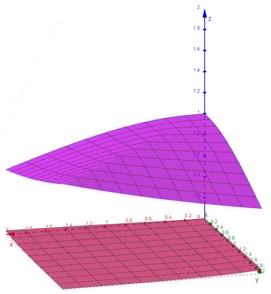
When , the terms of inequality (40) are
and
Now, we draw surfaces for the terms and in one figure when and in another figure when .
Then, from Figure 1, we see the inequality (40) satisfies in the interval , and from Figure 2, we see the inequality (40) satisfies in the interval .
Thus, (40) holds for all . That is, all hypotheses of Theorem 3 are satisfied, so A must fix a unique point. Clearly, is such point with .
The following remark will distinguish the Theorem 2 and 3.

Remark 1.
The inequality (40) in Theorem 3 will imply the inequality (1) in Theorem 2 only when either or in both cases. But we used the function g from different collection for both the theorems, where the collections is the set of all those functions g with the condition ⇒ and is the set of all those functions g with the condition ⇒, for , are completely different. So, we cannot compare the inequalities. Also, the term is different in both the theorems.
We now present some consequent results.
Corollary 1.
Let A be a self-mapping in a complete -metric space for such that satisfies
for all , where
Then, the mapping A fixes a unique point .
Proof.
For the defined sequence in Theorem 2, if , then
Consequently, the result follows Theorem 2. □
Corollary 2.
Let A be a self-mapping in a complete -metric space for such that satisfies
for all , where
Then, the mapping A fixes a unique point .
Proof.
Consequently, the result follows Theorem 3. □
For the defined sequence in Theorem 3, if , then
Corollary 3.
Let A be a self-mapping in a complete -metric space for such that satisfies
for all , where
Then, the mapping A fixes a unique point .
Proof.
For the defined sequence in Theorem 2, if , then
Consequently, the result follows Theorem 2. □
Corollary 4.
Let A be a self-mapping in a complete -metric space for such that satisfies
for all , where
Then, the mapping A fixes a unique point .
Proof.
For the defined sequence in Theorem 3, if , then
Consequently, the result follows Theorem 3. □
4. Application
When it comes to solving differential equations in mathematics, integral equations are usually crucial. FP methods have been utilized by numerous authors to solve integral problems. Within this framework of inquiry, we utilize Theorem 2 to determine whether the integral equation below has a solution. Consider the following integral equation
where and are continuous, is a function, and for all (see, [12,13]).
Let and be -metric given by
for all . Then, is an -metric space with regard to the parameter .
Let be given by
Now, we present a result for existence of a solution of (87).
Theorem 4.
Let the following conditions be met:
- (1)
- there exists for all
- (2)
- there exists withwhere
Then, the integral equation given in (87) has a unique solution.
5. Conclusions
In conclusion, following Geraghty [7] and Wang et al. [10] we presented a new type of Geraghty contraction and studied fixed point results within the framework of -metric space for these contractions which includes auxiliary functions with a restricted co-domain. This new idea of defining Geraghty contraction for self operators generalized a large number of previously published and closely related works for the presence and uniqueness of a fixed point in -metric space. We demonstrated that the self-operators that fulfill this contraction need to have only one fixed point. Additionally, we offer examples that explain on the obtained outcomes, and a utilization of the integral equation demonstrates how significant they are in the literature.
Author Contributions
Conceptualization, Y.R.; formal analysis, K.H.A., M.P.S., Y.R. and N.S.; investigation, Y.R., K.H.A., N.S. and K.A.S.; writing—original draft preparation, M.P.S. and K.H.A.; writing—review and editing, K.H.A., Y.R., A.R. and N.S. All authors have read and agreed to the publish current version of the manuscript.
Funding
This work was supported by the Deanship of Scientific Research, Vice Presidency for Graduate Studies and Scientific Research, King Faisal University, Saudi Arabia [Grant No. 5193].
Data Availability Statement
No new data were created or analyzed in this study. Data sharing is not applicable to this article.
Acknowledgments
The first author is supported by NIT Manipur, India.
Conflicts of Interest
The authors declare no conflict of interest.
References
- Banach, S. Sur les opérations dans les ensembles abstraits et leur applications aux èquations intégrales. Fund. Math. 1922, 3, 133–181. [Google Scholar] [CrossRef]
- Bakhtin, I.A. The contraction mapping principle in quasimetric spaces. Funct. Anal. 1989, 30, 26–37. [Google Scholar]
- Sedghi, S.; Shobe, N.; Aliouche, A. A generalization of fixed point theorems in S-metric spaces. Mat. Vesn. 2012, 64, 258–266. [Google Scholar]
- Rohen, Y.; Došenović, T.; Radenović, S. A Note on the Paper “A Fixed Point Theorems in Sb-Metric Spaces”. Filomat 2017, 31, 3335–3346. [Google Scholar] [CrossRef]
- Souayah, N.; Mlaiki, N. A fixed point theorem in Sb-metric spaces. J. Math. Comput. Sci. 2016, 16, 131–139. [Google Scholar] [CrossRef]
- Sedghi, S.; Gholidahneh, A.; Došenović, T.; Esfahani, J.; Radenović, S. Common fixed point of four maps in Sb-metric spaces. J. Linear Topol. Algebra 2016, 5, 93–104. [Google Scholar]
- Geraghty, M. On contractive mappings. Proc. Am. Math. Soc. 1973, 40, 604–608. [Google Scholar] [CrossRef]
- Aydi, H.; Felhi, A.; Afshari, H. New Geraghty type contractions on metric-like spaces. J. Nonlinear Sci. Appl. 2017, 10, 780–788. [Google Scholar] [CrossRef]
- Karapinar, E.; Alsulami, H.H.; Noorwali, M. Some extensions for Geraghty type contractive mappings. J. Inequal. Appl. 2015, 2015, 303. [Google Scholar] [CrossRef]
- Wang, Y.; Chen, C. Two new Geraghty type contractions in Gb-metric spaces. J. Funct. Spaces 2019, 2019, 7916486. [Google Scholar] [CrossRef]
- Alam, K.H.; Rohen, Y.; Saleem, N. Fixed points of (α, β, F*) and (α, β, F**)-weak Geraghty contractions with an application. Symmetry 2023, 15, 243. [Google Scholar] [CrossRef]
- Chidume, C.E.; Adamu, A.; Nnakwe, M.O. An Inertial Algorithm for Solving Hammerstein Equations. Symmetry 2021, 13, 376. [Google Scholar] [CrossRef]
- Chidume, C.E.; Adamu, A.; Minjibir, M.S.; Nnyaba, U.V. On the strong convergence of the proximal point algorithm with an application to Hammerstein euations. J. Fixed Point Theory Appl. 2020, 22, 61. [Google Scholar] [CrossRef]
Disclaimer/Publisher’s Note: The statements, opinions and data contained in all publications are solely those of the individual author(s) and contributor(s) and not of MDPI and/or the editor(s). MDPI and/or the editor(s) disclaim responsibility for any injury to people or property resulting from any ideas, methods, instructions or products referred to in the content. |
© 2023 by the authors. Licensee MDPI, Basel, Switzerland. This article is an open access article distributed under the terms and conditions of the Creative Commons Attribution (CC BY) license (https://creativecommons.org/licenses/by/4.0/).