Curves in Lightlike Planes in Three-Dimensional Lorentz–Minkowski Space

Abstract

In this paper, we analyze the intrinsic geometry of lightlike planes in the three-dimensional Lorentz–Minkowski space ${\mathbb{M}}^3$. We connect the theory of curves lying in lightlike planes in ${\mathbb{M}}^3$ with the theory of curves in the simply isotropic plane ${\mathbb{I}}^2$. Based on these relations, we characterize some special classes of curves that lie in lightlike planes in ${\mathbb{M}}^3$.

1. Introduction

In the three-dimensional Lorentz–Minkowski space ${\mathbb{M}}^3$, we distinguish three types of surfaces with respect to their induced metric—spacelike, timelike, or lightlike. Their metric is either positive definite, indefinite, or degenerate of rank 1, respectfully. The same holds for planes in ${\mathbb{M}}^3$, with the consequence that the intrinsic geometry of these planes is either Euclidean, pseudo-Euclidean (two-dimensional Lorentzian-Minkowskian), or isotropic in the sense developed by [1]. The geometry of lightlike planes and, then, also of its objects can be quite challenging to study, due to the degeneracy of the metric. However, they are still worthy of attention [2,3,4], since they are also important in the theory of general relativity. One of the known results is that every pseudo-null curve, that is a spacelike curve with a lightlike principal normal field, lies in a lightlike plane [5,6]. The aim of this paper was to relate the theory of curves lying in lightlike planes in ${\mathbb{M}}^3$ to the theory of curves in the simply isotropic space ${\mathbb{I}}^2$. This relationship was noted in [7], where we analyzed the involutes of pseudo-null curves. By obtaining the mentioned relationship, we can offer a new approach in the analysis of curves lying in lightlike planes, where we consider them as curves in an isotropic space ${\mathbb{I}}^2.$ As we will show, it turns out that the isotropic curvature of a curve can be more informative than its pseudo-torsion.

The paper is organized as follows. In Section 2, we recall the preliminaries of the Lorentz–Minkowski space and pseudo-null curves, as a special class of curves having lightlike fields in their Frenet bases. Then, we introduce a simply isotropic space ${\mathbb{I}}^n$, in particular two-dimensional ${\mathbb{I}}^2$, and describe the theory of curves in that space. In Section 3, we recall that pseudo-null curves lie in a lightlike plane and show that the converse also holds, that is every spacelike curve in a lightlike plane is pseudo-null. In Section 4, we define a Darboux frame of curves lying in a lightlike plane. In Section 5, we further develop connections between curves in lightlike planes and curves in simply isotropic space and give examples.

2. Preliminaries

2.1. Lorentz–Minkowski Space ${\mathbb{M}}^3$

The Lorentz–Minkowski three-space ${\mathbb{M}}^3$ is the three-dimensional vector space ${\mathbb{R}}^3$ equipped with the indefinite symmetric bilinear form of index 1 (a pseudo-scalar product):

$$\langle x,y\rangle =-x_1{y}_1+x_2{y}_2+x_3{y}_3.$$

A vector x in the Lorentz–Minkowski space ${\mathbb{M}}^3$ is called spacelike if $\langle x,x\rangle >0$ or $x=0$, timelike if $\langle x,x\rangle <0$, and lightlike (null, isotropic) if $\langle x,x\rangle =0$ and $x\ne 0$. The pseudo-norm of a vector x is defined as the real number:

$$\parallel x\parallel =\sqrt{|\langle x,x\rangle |}\ge 0.$$

There exist locally three types of curves and surfaces in ${\mathbb{M}}^3$: spacelike, timelike, and lightlike (null). The type of a curve is defined based on the character of its tangent vectors, whereas the type of a surface with respect to the induced metric, either as having the induced metric positive definite, indefinite, or degenerate of rank 1, respectively. We can note that the type of a surface is characterized by the causal character of its normal vectors, which are timelike, spacelike, and lightlike, respectively [8,9].

In this paper, we are interested in lightlike surfaces in ${\mathbb{M}}^3$. If S is a regular lightlike surface in ${\mathbb{M}}^3$ and $T_{p}S$ its tangent plane, $p\in S$, then by $T_p{S}^{\perp }$, we denote the space of all vectors orthogonal to the tangent vectors at p:

$$T_p{S}^{\perp }=\{w\in T_p{\mathbb{M}}^3:\langle v,w\rangle =0,\forall v\in T_{p}S\}.$$

In contrast to non-degenerate surfaces, the union of $T_{p}S$ and $T_p{S}^{\perp }$ for lightlike surfaces is not the whole $T_p{\mathbb{M}}^3$; timelike vectors cannot be contained either in a lightlike plane $T_{p}S$ or in its complement $T_p{S}^{\perp }$ (timelike vectors cannot be orthogonal to lightlike) [9]. Besides, the intersection of $T_{p}S$ and $T_p{S}^{\perp }$ is not trivial, since a lightlike tangent vector is orthogonal to itself. Therefore, the subspace:

$$Rad{T}_{p}S:=T_{p}S\cap T_p{S}^{\perp }$$

is introduced and called the radical subspace of S at the point p. Since $T_p{S}^{\perp }$ is a 1-dimensional lightlike subspace, then $Rad{T}_{p}S$ is also a 1-dimensional lightlike subspace:

$$Rad{T}_{p}S=T_p{S}^{\perp }\subseteq T_{p}S.$$

To summarize, in each tangent plane of a lightlike surface, there exists a unique lightlike direction determined by $v\in Rad{T}_{p}S$, $v\ne 0$. We use $Rad{T}_{p}S$ instead of $T_p{S}^{\perp }$ and refer to normal vectors of a lightlike surface S as the vectors of the radical space of S (see [2,3,4]).

Furthermore, the decomposition:

$$T_{p}S=Rad{T}_{p}S\perp S\left(T_{p}S\right)$$

defines a vector subspace $S\left(T_{p}S\right)$, the so-called screen distribution of S, as the orthogonal complementary vector space of $Rad{T}_{p}S$ in $T_{p}S$. A screen distribution $S\left(T_{p}S\right)$ is a spacelike vector space of dimension one. It is important to notice that it is not unique, and therefore, the geometry of a lightlike surface generally depends on its choice. Furthermore, for a given screen distribution $S\left(T_{p}S\right)$, there exists a unique complementary vector space $ltr\left(T_{p}S\right)$ called the lightlike transversal space of S. It is of dimension one, and $T_p{\mathbb{M}}^3$ now splits into

$$T_p{\mathbb{M}}^3{|}_S=T_{p}S\oplus ltr\left(T_{p}S\right)=(Rad{T}_{p}S\perp S\left(T_{p}S\right))\oplus ltr\left(T_{p}S\right).$$

2.2. Pseudo-Null Curves in Lorentz–Minkowski Space ${\mathbb{M}}^3$

Pseudo-null curves in ${\mathbb{M}}^3$ are spacelike curves having their principal normals lightlike, and therefore, their binormals are lightlike as well. We recall their Frenet frames and curvatures in ${\mathbb{M}}^3$.

Let c be a pseudo-null curve in ${\mathbb{M}}^3$ parametrized by arc-length $\parallel c^{\prime }\left(s\right)\parallel =\parallel \mathbf{t}\left(s\right)\parallel =1$, $s\in I$. Its Frenet frame $\{\mathbf{t},\mathbf{n},\mathbf{b}\}$ forms a pseudo-orthonormal basis (also called a lightlike basis), with the lightlike principal normal vector field $\mathbf{n}$ defined as $\mathbf{n}\left(s\right)=c^{″}\left(s\right)$ and the lightlike binormal $\mathbf{b}\left(s\right)$ satisfying $\langle \mathbf{t},\mathbf{b}\rangle =0$, $\langle \mathbf{n},\mathbf{b}\rangle =1$. The Frenet equations are given by

$$\left(\begin{array}{c}{\mathbf{t}}^{\prime }\\ {\mathbf{n}}^{\prime }\\ {\mathbf{b}}^{\prime }\end{array}\right)=\left(\begin{array}{ccc}0& \kappa & 0\\ 0& \tau & 0\\ -\kappa & 0& -\tau \end{array}\right)\left(\begin{array}{c}\mathbf{t}\\ \mathbf{n}\\ \mathbf{b}\end{array}\right).$$

(1)

The function $\kappa$ takes only two values, 0 if c is a straight line or 1 otherwise. The function $\tau =\langle {\mathbf{n}}^{\prime },\mathbf{b}\rangle$ is called the pseudo-torsion [9,10].

2.3. Darboux Frames of Curves on Lightlike Surfaces

In the classical differential geometry, a Darboux frame is defined as a moving frame adapted for curves lying on a certain surface. It reflects the geometry of curves by conditions imposed from a surface.

In Euclidean space, a Darboux frame of a curve lying on a surface consists of a tangent field $\mathbf{t}$ of a curve, a surface unit normal $\mathbf{u}$, and a so-called side-tangential field $\mathbf{q}$, that is their vector product. Derivatives of these fields yield functions called curvatures, the geodesic curvature ${\kappa }_g$, the normal curvature ${\kappa }_n$, and the geodesic torsion ${\tau }_g$, that is the following holds:

$$\left(\begin{array}{c}{\mathbf{t}}^{\prime }\\ {\mathbf{q}}^{\prime }\\ {\mathbf{u}}^{\prime }\end{array}\right)=\left(\begin{array}{ccc}0& {\kappa }_g& {\kappa }_n\\ -{\kappa }_n& 0& {\tau }_g\\ -{\kappa }_g& -{\tau }_g& 0\end{array}\right)\left(\begin{array}{c}\mathbf{t}\\ \mathbf{q}\\ \mathbf{u}\end{array}\right).$$

(2)

The vanishing of these curvatures describes curves on a surface known as geodesic curves, asymptotic curves, and principal curves (lines of curvature), respectively.

In this paper, we consider curves lying on a lightlike plane in three-dimensional Lorentz–Minkowski space. If a curve lies on an arbitrary lightlike surface, its Darboux frame is introduced in [11,12] as follows. Let c be a unit-speed curve lying on a lightlike surface S in Lorentz–Minkowski space ${\mathbb{M}}^3$, $\mathbf{t}=c^{\prime }$. Let $\mathbf{u}$ be a lightlike field in $RadTS$ and $\mathbf{q}$ a unique lightlike field (lightlike transversal field) such that the following orthogonality conditions hold:

$$\langle \mathbf{t},\mathbf{t}\rangle =\langle \mathbf{u},\mathbf{q}\rangle =1,\langle \mathbf{u},\mathbf{u}\rangle =\langle \mathbf{q},\mathbf{q}\rangle =\langle \mathbf{t},\mathbf{u}\rangle =\langle \mathbf{t},\mathbf{q}\rangle =0.$$

Further, the following formulas are satisfied:

$$\left(\begin{array}{c}{\mathbf{t}}^{\prime }\\ {\mathbf{u}}^{\prime }\\ {\mathbf{q}}^{\prime }\end{array}\right)=\left(\begin{array}{ccc}0& {\kappa }_g& {\kappa }_n\\ -{\kappa }_n& {\tau }_g& 0\\ -{\kappa }_g& 0& -{\tau }_g\end{array}\right)\left(\begin{array}{c}\mathbf{t}\\ \mathbf{u}\\ \mathbf{q}\end{array}\right).$$

(3)

2.4. Curves in an Isotropic Space ${\mathbb{I}}^n$

Isotropic space ${\mathbb{I}}^n$ is the vector space ${\mathbb{R}}^n$ equipped with the degenerate symmetric bilinear form (a degenerate scalar product) of rank $n-1$:

$${\langle x,y\rangle }_{\mathbb{I}}=x_1{y}_1+\dots +x_{n-1}{y}_{n-1}.$$

It is called an isotropic scalar product and also referred to as the “top-view product” since it coincides with the Euclidean scalar product of the projections of vectors onto the first $(n-1)$-coordinates. The isotropic scalar product generates the isotropic norm in the usual way ${\parallel x\parallel }_{\mathbb{I}}=\sqrt{{\langle x,x,\rangle }_{\mathbb{I}}}$. Vectors collinear to $(0,0,\dots ,1)$, for which the isotropic norm vanishes, are called isotropic vectors. They generate a unique isotropic direction in ${\mathbb{I}}^n$. The other vectors are called non-isotropic.

A curve in ${\mathbb{I}}^n$ that is not an isotropic line, that is its tangent vectors, are all non-isotropic and can be (re)parametrized by arc-length, $\parallel c^{\prime }{\left(s\right)\parallel }_{\mathbb{I}}=1$, in the usual way. This is called admissible, since it allows the construction of the Frenet frame.

In the special case of the isotropic plane ${\mathbb{I}}^2$, a curve $c\left(s\right)=\left(x\right(s),y(s\left)\right)$ is parametrized by the arc-length if $x^{\prime }\left(s\right)=\pm 1$. We shall, for instance, take $c\left(s\right)=(s,y(s\left)\right).$ For curves parametrized by the arc-length in ${\mathbb{I}}^2$, the Frenet frame is introduced by ${\mathbf{t}}_{\mathbb{I}}=c^{\prime }$, ${\mathbf{n}}_{\mathbb{I}}=(0,1)$, and the following Frenet formulas hold:

$$\left(\begin{array}{c}{\mathbf{t}}_{\mathbb{I}}^{\prime }\\ {\mathbf{n}}_{\mathbb{I}}^{\prime }\end{array}\right)=\left(\begin{array}{cc}0& {\kappa }_{\mathbb{I}}\\ 0& 0\end{array}\right)\left(\begin{array}{c}{\mathbf{t}}_{\mathbb{I}}\\ {\mathbf{n}}_{\mathbb{I}}\end{array}\right).$$

The isotropic curvature ${\kappa }_{\mathbb{I}}$ is determined as

$${\kappa }_{\mathbb{I}}=det(c^{\prime },c^{″})=y^{″}\left(s\right).$$

(4)

If c is parametrized by an arbitrary parameter, then

$${\kappa }_{\mathbb{I}}\left(t\right)=\frac{det(c^{\prime }\left(t\right),c^{″}\left(t\right))}{x_1^{\prime }{\left(t\right)}^3}.$$

A circle in an isotropic plane is a regular curve of the second order with a normal equation $y=R{x}^2$. The real number R is defined as its radius. As a curve, it is a Euclidean parabola, whose axis coincides with the isotropic direction.

Remark 1.

Considering the geometry of an isotropic plane ${\mathbb{I}}^2$ as a Cayley–Klein geometry ([1], p. 23), a circle is defined as a regular curve of the second order in the underlying projective plane, which contains the absolute point F of ${\mathbb{I}}^2$ and touches the absolute line in F. This implies that, in affine coordinates, a circle is a curve with the given normal equation.

Remark 2

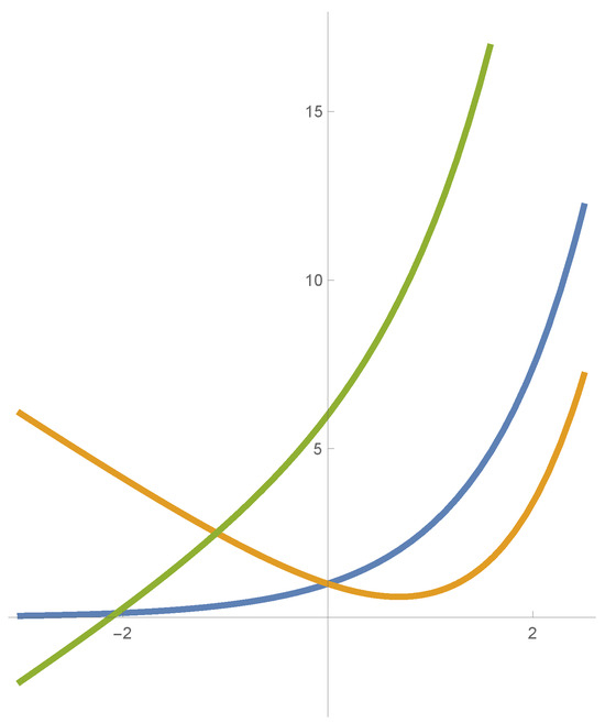
([1]). The fundamental theorem for curves in ${\mathbb{I}}^2$ states that, with the given isotropic curvature ${\kappa }_{\mathbb{I}}\left(s\right)$, there exists, up to isotropic motions, a unique curve parametrized by arc-length s with the given curvature. Note that, in particular, curves $c\left(s\right)=(s,f(s\left)\right)$, $\overline{c}\left(s\right)=(s,f\left(s\right)+as+b)$, $a,b,\in \mathbb{R}$, are congruent, which does not hold in the Euclidean plane (see the example in Figure 1).

In an isotropic plane, the following curves are characterized by constant isotropic curvature.

Proposition 1

([1]). Let $c:I\to {\mathbb{I}}^2$ be a non-isotropic curve in an isotropic plane ${\mathbb{I}}^2$. Then:

1. 

${\kappa }_{\mathbb{I}}=0$ on I if and only if c is a non-isotropic straight line;

2. 

${\kappa }_{\mathbb{I}}=const.\ne 0$ on I if and only if c is an isotropic circle.

3. Pseudo-Null Curves in ${\mathbb{M}}^{\mathbf{3}}$ Are Planar Curves

We begin this section by offering an alternative proof of the fact that every pseudo-null curve lies in a lightlike plane. A different proof of this property can be found in [5,6].

Proposition 2.

A pseudo-null curve with the curvature $\kappa \left(s\right)=1$ is a planar curve lying in a lightlike plane.

Proof. 

Let the principal normal vector field $\mathbf{n}$ of a pseudo-null curve c parametrized by the arc-length be written as $\mathbf{n}=(n_1,n_2,n_3).$ Since $\mathbf{n}=c^{″}$ and by the Frenet equation ${\mathbf{n}}^{\prime }=\tau \mathbf{n}$ in (1), we can conclude that

$$n_i=K_i{e}^{\int \tau \left(s\right)ds},K_i\in \mathbb{R},i=1,2,3,$$

with $K_1\ne 0$ since $\mathbf{n}$ is lightlike. Therefore,

$$\mathbf{n}=e^{\int \tau \left(s\right)ds}(K_1,K_2,K_3),$$

(5)

where the vector:

$$\mathbf{u}\left(s\right)=(K_1,K_2,K_3)\ne 0,$$

is a constant lightlike vector. We consider a function

$$f\left(s\right)=\langle c\left(s\right)-c\left(s_0\right),\mathbf{u}\left(s\right)\rangle ,$$

for an arbitrary $s_0\in I$. Since $\mathbf{u}$ is constant, we have $f^{\prime }\left(s\right)=\langle \mathbf{t}\left(s\right),\mathbf{u}\left(s\right)\rangle =0$, so f is a constant function. Since $f\left(s_0\right)=0$ and f is smooth, we can conclude that $f\left(s\right)=0$ for all s. This means that c lies in a plane with the equation $\langle \mathbf{x}-c\left(s_0\right),\mathbf{u}\left(s\right)\rangle =0$. □

Remark 3.

The normal field $\mathbf{u}$ belongs to the radical space $Ra{d}_{p}S=T_p{S}^{\perp }$ of a lightlike plane S. Obviously, a constant vector $\mathbf{u}$ in the previous proposition is determined up to a multiplicative constant.

Remark 4.

A pseudo-null curve lies in a plane through an arbitrary point of a curve spanned by (linearly independent) $c^{\prime }\left(s\right)=\mathbf{t},c^{″}\left(s\right)=\mathbf{n}$. Notice that this is a consequence of the fact that $c^{‴}\left(s\right)$ is linearly dependent with $c^{\prime }\left(s\right),c^{″}\left(s\right)$. The same holds for planar non-degenerate curves. We refer to this plane as the osculating plane (being spanned by $\mathbf{t},\mathbf{n}$), whereas some authors call it a rectifying plane (as having a normal $\mathbf{n}$).

Pseudo-null curves lie in planes that are lightlike, having a lightlike direction determined by $c^{″}\in Rad\left(TS\right)$. This additional fact that the osculating plane is lightlike for pseudo-null curves is characterized by the vanishing Gram determinant (with respect to the pseudo-scalar product of ${\mathbb{M}}^3$) [13]:

$$\Gamma (c^{\prime },c^{″})=\left|\begin{array}{cc}\langle c^{\prime },c^{\prime }\rangle & \langle c^{\prime },c^{″}\rangle \\ \langle c^{\prime },c^{″}\rangle & \langle c^{″},c^{″}\rangle \end{array}\right|=0.$$

We can verify this first for pseudo-null curves c parametrized by the arc-length, $\langle c^{\prime },c^{\prime }\rangle =1$. Then, also, $\langle c^{\prime },c^{″}\rangle =0.$ Additionally, the principal normals are lightlike, $\langle c^{″},c^{″}\rangle =0.$ Therefore, we conclude

$$\Gamma (c^{\prime },c^{″})=\left|\begin{array}{cc}1& 0\\ 0& 0\end{array}\right|=0.$$

If c is parametrized by an arbitrary parameter t and $\overline{c}$ is its reparametrization by the arc-length parameter s, then $c^{\prime }\left(t\right)={\overline{c}}^{\prime }\left(s\right)\frac{ds}{dt}$, $c^{″}\left(t\right)={\overline{c}}^{″}\left(s\right){\left(\frac{ds}{dt}\right)}^2+{\overline{c}}^{\prime }\left(s\right)\frac{d^{2}s}{d{t}^2}$. Then, also,

$$\Gamma (c^{\prime },c^{″})=\left|\begin{array}{cc}{\left(\frac{ds}{dt}\right)}^2& \frac{ds}{dt}\frac{d^{2}s}{d{t}^2}\\ \frac{ds}{dt}\frac{d^{2}s}{d{t}^2}& {\left(\frac{d^{2}s}{d{t}^2}\right)}^2\end{array}\right|=0.$$

Finally, note that, by the Lagrange identity in ${\mathbb{M}}^3$, we have

$$\Gamma (c^{\prime },c^{″})={\langle c^{\prime },c^{″}\rangle }^2-\langle c^{\prime },c^{\prime }\rangle \langle c^{″},c^{″}\rangle =\langle c^{\prime }\times c^{″},c^{\prime }\times c^{″}\rangle ,$$

where × is the Lorentzian cross-product ([9]). The vector $c^{\prime }\times c^{″}$ is a vector orthogonal to both $c^{\prime },$ $c^{″}$. In the case of non-degenerate surfaces, it is a surface normal. However, for lightlike planes, it is an element of the radical space of S, being lightlike and orthogonal to a lightlike direction of S.

4. Curves in a Lightlike Plane in ${\mathbb{M}}^{\mathbf{3}}$

A lightlike plane S is a lightlike surface in Lorentz–Minkowski space ${\mathbb{M}}^3$, and its radical space is determined by a unique lightlike direction; we denote it by $\mathbf{u}$. This means that $RadS=span\left\{u\right\}$.

Let $c:I\subset \mathbb{R}\to {\mathbb{M}}^3$ be a curve that lies in S. If we assume that the causal character of c does not change on I, then c is either a lightlike curve or a spacelike curve. If c is a lightlike curve, then it has the same direction as the lightlike direction $\mathbf{u}$. Let c be a spacelike curve in S with the curvature $\kappa =1$. Then, a vector field $\mathbf{t}=c^{\prime }$ is spacelike, and there exists a unique lightlike field $\mathbf{q}$ satisfying

$$\langle \mathbf{q},\mathbf{q}\rangle =0,\langle \mathbf{t},\mathbf{q}\rangle =0,\langle \mathbf{u},\mathbf{q}\rangle =1.$$

In the following, we frame c by the pseudo-orthonormal frame $L=(\mathbf{t},\mathbf{u},\mathbf{q})$ as a Darboux frame for a lightlike plane.

Theorem 1.

Let $L=(\mathbf{t},\mathbf{u},\mathbf{q})$ be a Darboux frame of a curve c, the spacelike curve c, with the curvature $\kappa =1$ lying in a lightlike plane S. Then, the following holds:

$$\left(\begin{array}{c}{\mathbf{t}}^{\prime }\\ {\mathbf{u}}^{\prime }\\ {\mathbf{q}}^{\prime }\end{array}\right)=\left(\begin{array}{ccc}0& {\kappa }_g& 0\\ 0& 0& 0\\ -{\kappa }_g& 0& 0\end{array}\right)\left(\begin{array}{c}\mathbf{t}\\ \mathbf{u}\\ \mathbf{q}\end{array}\right)$$

(6)

where ${\kappa }_g$ is a function defined as

$${\kappa }_g=\langle {\mathbf{t}}^{\prime },\mathbf{q}\rangle =-\langle \mathbf{t},{\mathbf{q}}^{\prime }\rangle .$$

(7)

Proof. 

Let us put ${\mathbf{t}}^{\prime }=\alpha \mathbf{t}+\beta \mathbf{u}+\gamma \mathbf{q}$, where, for the unknown functions $\alpha ,\beta ,\gamma :I\to \mathbb{R}$, it holds that $\alpha =\langle {\mathbf{t}}^{\prime },\mathbf{t}\rangle ,$$\beta =\langle {\mathbf{t}}^{\prime },\mathbf{q}\rangle ,$$\gamma =\langle {\mathbf{t}}^{\prime },\mathbf{u}\rangle .$ Since $\langle \mathbf{t},\mathbf{t}\rangle =1$, and we have $\langle {\mathbf{t}}^{\prime },\mathbf{t}\rangle =0$, so $\alpha =0.$ From $\langle \mathbf{t},\mathbf{u}\rangle =0$ and because $\mathbf{u}$ is constant, we obtain $\langle {\mathbf{t}}^{\prime },\mathbf{u}\rangle =0$, so $\gamma =0$. Therefore, we may write ${\mathbf{t}}^{\prime }=\beta \mathbf{u}$. For the function $\beta$, we put $\beta :={\kappa }_g$.

The second formula follows because $\mathbf{u}$ is a constant vector. For the third formula, we have the following: if we write ${\mathbf{q}}^{\prime }=\overline{\alpha }\mathbf{t}+\overline{\beta }\mathbf{u}+\overline{\gamma }\mathbf{q}$, for the unknown functions $\overline{\alpha },\overline{\beta },\overline{\gamma }:I\to \mathbb{R}$, it holds that $\overline{\alpha }=\langle {\mathbf{q}}^{\prime },\mathbf{t}\rangle ,$$\overline{\beta }=\langle {\mathbf{q}}^{\prime },\mathbf{q}\rangle ,$$\overline{\gamma }=\langle {\mathbf{q}}^{\prime },\mathbf{u}\rangle .$ Since $\mathbf{q}$ is a lightlike vector, $\langle \mathbf{q},\mathbf{q}\rangle =0$, then $\langle {\mathbf{q}}^{\prime },\mathbf{q}\rangle =0$, so $\overline{\beta }=0$. From $\langle \mathbf{u},\mathbf{q}\rangle =1$, it follows that $\langle \mathbf{u},{\mathbf{q}}^{\prime }\rangle =0$; therefore, $\overline{\gamma }=0$. Finally, since $\langle \mathbf{t},\mathbf{q}\rangle =0$, we have ${\kappa }_g=\langle {\mathbf{t}}^{\prime },\mathbf{q}\rangle =-\langle \mathbf{t},{\mathbf{q}}^{\prime }\rangle$, which gives $\overline{\alpha }=-{\kappa }_g$. □

Remark 5.

We note that the formulas (6) for lightlike planes appear as the special case of the formulas for the Darboux frame (3) for a general lightlike surface with ${\kappa }_n={\tau }_g=0$.

By Proposition 2, we know that a pseudo-null curve lies in a lightlike plane. Now, we consider the converse: Which curves lie in a lightlike plane?

Corollary 1.

Every spacelike curve with the curvature $\kappa =1$ that lies in a lightlike plane in ${\mathbb{M}}^3$ is a pseudo-null curve.

Proof. 

Without loss of generality, we may assume that c is parametrized by the arc-length. From the formulas (6), we have $c^{″}=t^{\prime }={\kappa }_g\mathbf{u}$. If ${\kappa }_g$ is different from zero, $c^{″}$ is a lightlike vector, and c is a pseudo-null curve. □

5. Connection between the Frenet and Darboux Frames of a Pseudo-Null Curve

Our next goal is to determine the relations between two constructed frames (1) and (6) for a pseudo-null curve (parametrized by the arc-length) and their curvatures, the curvature $\kappa$, the pseudo-torsion $\tau$, and the geodesic curvature ${\kappa }_g$.

First note that the tangent field $\mathbf{t}$ is the same in both frames. Let us first consider the case of spacelike straight lines. A curve c is a spacelike straight line if and only if its curvature $\kappa$ as a pseudo-null curve in ${\mathbb{M}}^3$ vanishes, $\kappa =0$ (see (1)). Likewise, $c^{″}={\mathbf{t}}^{\prime }={\kappa }_g\mathbf{u}=0$ implies ${\kappa }_g=0.$ Therefore, in this case, we have

$$\kappa ={\kappa }_g=0.$$

Otherwise, ${\kappa }_g$ is related to the pseudo-torsion $\tau$, which we discuss further on. Let now $c=c\left(s\right)$ be a pseudo-null curve with the curvature $\kappa =1$, and let it be parametrized by arc-length s. Let $\mathbf{u}$ be a constant vector in the direction of the principal normal vector $\mathbf{n}=c^{″}$ of c (see (5)). Note that the vector $\mathbf{u}$ is determined up to a multiplicative constant. With the vector $\mathbf{u}$ chosen and fixed, by (6), we may write

$$c^{″}\left(s\right)={\mathbf{t}}^{\prime }\left(s\right)=\mathbf{n}\left(s\right)={\kappa }_g\left(s\right)\mathbf{u}\left(s\right),$$

(8)

which by (5) implies

$${\kappa }_g\left(s\right)=e^{\int \tau \left(s\right)ds},$$

(9)

or

$$\tau =\frac{{\kappa }_g^{\prime }}{{\kappa }_g}.$$

(10)

Lightlike normal fields $\mathbf{u},\mathbf{n}$ are, therefore, related as follows:

$$\mathbf{u}\left(s\right)=e^{-\int \tau \left(s\right)ds}\mathbf{n}\left(s\right)=\frac{1}{{\kappa }_g\left(s\right)}{c}^{″}\left(s\right).$$

(11)

Furthermore, since $\langle \mathbf{n},\mathbf{b}\rangle =\langle \mathbf{u},\mathbf{q}\rangle =1$, then $\mathbf{q},$ $\mathbf{b}$ are related as follows:

$$\mathbf{q}\left(s\right)={\kappa }_g\left(s\right)\mathbf{b}\left(s\right).$$

(12)

Summarizing:

Proposition 3.

Let c be a pseudo-null curve with the curvature $\kappa =1$ and the Frenet pseudo-orthonormal frame $(\mathbf{t},\mathbf{n},\mathbf{b})$ satisfying (1). Then, its Darboux frame $(\mathbf{t},\mathbf{u},\mathbf{q})$ is defined by (11), (12), and ${\kappa }_{\mathbb{I}}$ and τ are related by (9).

Remark 6.

In Euclidean space, curvatures from the Frenet and Darboux frame for curves parametrized by the arc-length are connected by ${\kappa }_g=\kappa cos\phi$, ${\kappa }_n=-\kappa sin\phi$, ${\tau }_g=\tau +{\phi }^{\prime }$, where φ is the angle of rotation in the plane spanned by $\mathbf{n},\mathbf{b}$, which maps $\mathbf{n},\mathbf{b}$ to $\mathbf{q},\mathbf{u}$. In the case when a surface S is a plane, the field $\mathbf{b}$ is constant and represents a unit normal of a plane. It is equal to $\mathbf{u}$, up to a sign. The angle of rotation is constant (equal to $0,\pi$), and ${\kappa }_g$ coincides with κ, whereas other curvatures vanish.

6. Connection between Theories of Curves in ${\mathbb{I}}^2$ and in Lightlike Planes in ${\mathbb{M}}^3$: Examples

We introduce local coordinates in a lightlike plane $S\subset {\mathbb{M}}^3$. Since there is a unique lightlike direction in S, we can consider S as being given by passing through a point q and spanned by a lightlike vector $\mathbf{u}$ and a unit spacelike vector $\mathbf{v}$, that is given by a parametrization:

$$F(v,u)=q+v\mathbf{v}+u\mathbf{u}.$$

(13)

With respect to this parametrization, the induced metric of S is given with the coefficients $E=1$, $F=0$, $G=0$, that is $d{s}^2=d{v}^2$. The metric is degenerate of index 1.

We note that the vectors $\mathbf{v}$, $\mathbf{u}$ form constant fields of tangent vectors, $\mathbf{v}\in T_{p}S$, $\mathbf{u}\in Rad\left(T_p\right)\subset T_{p}S$, $p\in S$, which are orthogonal for every $p\in S$. The field $\mathbf{v}$ generates the screen distribution $S\left(TS\right)$. Its choice is not unique, since every spacelike vector in $T_{p}S$ is orthogonal to $\mathbf{u}$, $p\in S$. With the fields $\mathbf{v}$, $\mathbf{u}$ chosen and fixed, every point $x\in S$ can be given by the local coordinates in the plane S as $x=(v_0,u_0)$, after identification with $F(v_0,u_0).$

By this identification for a pseudo-null curve, we may write ${\kappa }_g={\kappa }_{\mathbf{I}}$. Indeed, for a pseudo-null curve c lying in its osculating plane spanned by $(\mathbf{v}$, $\mathbf{u}),$ i.e., by $(\mathbf{t}$, $\mathbf{n}),$ through a point q (see (13)), there exist functions $\alpha \left(s\right)$, $\beta \left(s\right)$ such that

$$c\left(s\right)=q+\alpha \left(s\right)\mathbf{v}+\beta \left(s\right)\mathbf{u}.$$

(14)

If c is parametrized by the arc-length, $\parallel c^{\prime }\left(s\right)\parallel ={\alpha }^{\prime }{\left(s\right)}^2=1$, implies $\alpha \left(s\right)=\pm s+c$. Following [1], without loss of generality, we will choose $\alpha \left(s\right)=s$. Now, (7) implies ${\kappa }_g=\langle {\mathbf{t}}^{\prime },\mathbf{q}\rangle ={\beta }^{″}\left(s\right)$. The same is obtained for a curve $c\left(s\right)=(s,\beta (s\left)\right)$ as a curve in ${\mathbf{I}}^2$, ${\kappa }_{\mathbf{I}}={\beta }^{″}\left(s\right)$ (see (4)).

Next, we are interested in understanding how the choice of the pseudo-orthonormal frame of constant fields $\mathbf{v}$, $\mathbf{u}$ (which determines the local coordinates) affects the isotropic curvature given by (4) of a curve c in a lightlike plane S.

Proposition 4.

Rescaling a constant field $\mathbf{u}$ by a constant has an effect on the isotropic curvature. If we put $\overline{\mathbf{u}}=a\mathbf{u}$, $a\in \mathbb{R}$, $a\ne 0$, then the corresponding isotropic curvature are related in the following way:

$${\overline{\kappa }}_{\mathbb{I}}=\frac{1}{a}{\kappa }_{\mathbb{I}}.$$

Proof. 

By introducing a frame $(\mathbf{v},\overline{\mathbf{u}})$, a curve c given by (14) and parametrized by arc-length, can be written as $c\left(s\right)=q+s\mathbf{v}+(1/a)\beta \overline{\mathbf{u}}$, that is with coordinates $c\left(s\right)=(s,(1/a\left)\beta \right)$ in the local frame. Since a is a constant, the isotropic curvature of c with respect to this frame is ${\overline{\kappa }}_{\mathbb{I}}=(1/a){\beta }^{″}$. □

Proposition 5.

The curvature ${\kappa }_{\mathbb{I}}$ does not depend on different choices of the constant unit spacelike field $\mathbf{v}$ (different screen distributions).

Proof. 

Let $(\mathbf{v},\mathbf{u})$, $(\overline{\mathbf{v}},\mathbf{u})$ be two pseudo-orthonormal frames consisting of constant fields, a unit spacelike field $\mathbf{v}$, respectively $\overline{\mathbf{v}}$, and a lightlike field $\mathbf{u}$. Obviously $\mathbf{v}=\overline{\mathbf{v}}+\lambda \mathbf{u}$, for a constant $\lambda \in \mathbb{R}$. Let $c:I\to S$ be a curve in S parametrized by the arc-length; see (14). Then, the unit tangent vector $\mathbf{t}$ of c is given by $\mathbf{t}=\mathbf{v}+f\left(s\right)\mathbf{u}$, or with respect to this basis in local coordinates

$$\mathbf{t}=(1,f(s\left)\right).$$

Similarly,

$$\mathbf{t}=\overline{\mathbf{v}}+(f\left(s\right)+\lambda )\mathbf{u}=(1,f\left(s\right)+\lambda ),$$

respectively. Now, we have ${\kappa }_{\mathbb{I}}=f^{\prime }\left(s\right)$, ${\overline{\kappa }}_{\mathbb{I}}={(f\left(s\right)+\lambda )}^{\prime }=f^{\prime }\left(s\right)$ which proves the claim. □

Based on these results and the theory of curves in an isotropic plane developed in [1], we analyzed some special pseudo-null curves in ${\mathbb{M}}^3$. By Proposition 1, we may conclude the following:

Theorem 2.

Let $c:I\to {\mathbb{M}}^3$ be a pseudo-null curve curve in ${\mathbb{M}}^3$. Then:

1. 

$\kappa =0$ on I if and only if c is a spacelike straight line;

2. 

$\tau =0$ on I if and only if c is an isotropic circle (a Euclidean parabola with the lightlike axis).

We are further interested in the class of spherical pseudo-null curves. These results can also be found in [14,15,16] and in [17] in the case of lightlike cones. In Lorentz–Minkowski space ${\mathbb{M}}^3$, the following sets are considered as spheres:

$$\begin{array}{ccc}\hfill {\mathbb{S}}_1^2(p,r)& =& \{q\in {\mathbb{M}}^3:\langle q-p,q-p\rangle =r^2\},\hfill \\ \hfill {\mathbb{H}}^2(p,r)& =& \{q\in {\mathbb{M}}^3:\langle q-p,q-p\rangle =-r^2\},\hfill \\ \hfill \mathbb{LC}\left(p\right)& =& \{q\in {\mathbb{M}}^3:\langle q-p,q-p\rangle =0\}.\hfill \end{array}$$

The set ${\mathbb{S}}_1^2(p,r)$ is called the Lorentzian sphere or a pseudo-sphere with center p and radius $r>0,$ the set ${\mathbb{H}}^2(p,r)$ a hyperbolic plane with center p and radius $r>0$, and the set $\mathbb{LC}\left(p\right)$ a lightlike cone with the vertex p. For unit spheres, we put ${\mathbb{S}}_1^2\left(p\right)={\mathbb{S}}_1^2(p,1),{\mathbb{H}}_1^2\left(p\right)={\mathbb{H}}_1^2(p,1).$

Proposition 6.

A pseudo-null curve that is spherical in ${\mathbb{M}}^3$, i.e., that lies on ${\mathbb{H}}^2\left(p\right)$, ${\mathbb{S}}_1^2\left(p\right)$, or $\mathbb{LC}\left(p\right)$, $p\in {\mathbb{M}}^3$, is an isotropic circle (a Euclidean parabola).

Proof. 

First, we assume that a pseudo-null curve c parametrized by the arc-length parameter lies on ${\mathbb{H}}^2\left(p\right)$, ${\mathbb{S}}_1^2\left(p\right)$, or $\mathbb{LC}\left(p\right)$. Therefore,

$$\langle c\left(s\right)-p,c\left(s\right)-p\rangle =\epsilon ,\epsilon \in \{\pm 1,0\}.$$

Differentiating the previous expression twice, we obtain $\langle c\left(s\right)-p,\mathbf{t}\rangle =0$, $\langle \mathbf{t},\mathbf{t}\rangle +\langle c\left(s\right)-p,\mathbf{n}\rangle =0$. Hence, by using (8) and ${\kappa }_{\mathbb{I}}={\kappa }_g$, we obtain

$${\kappa }_{\mathbb{I}}\langle c\left(s\right)-p,\mathbf{u}\rangle =-1.$$

(15)

Further, we represent c by (14). By taking the pseudo-scalar product of (14) by $\mathbf{u}$, we obtain $\langle c\left(s\right)-q,\mathbf{u}\rangle =0$. Therefore, $\langle c\left(s\right)-p,\mathbf{u}\rangle =\langle q-p,\mathbf{u}\rangle =const.\ne 0$, since $q\ne p$. Now, (15) implies

$${\kappa }_{\mathbb{I}}=-\frac{1}{\langle q-p,\mathbf{u}\rangle },$$

and from Proposition 1, it follows that c is an isotropic circle.

In the case when the osculating plane passes through the center of a sphere, $q=p$, then the relation (14) implies $\langle c\left(s\right)-p,c\left(s\right)-p\rangle =\langle c\left(s\right)-q,c\left(s\right)-q\rangle ={\alpha }^2\left(s\right)=\epsilon ,\epsilon \in \{\pm 1,0\}.$ In the case $\epsilon =-1$, we have ${\alpha }^2=-1$ with $\alpha \in \mathbb{R}$, which implies that there is no intersection of ${\mathbb{H}}^2\left(p\right)$ by a lightlike plane passing through its center. In the case when $\epsilon =1$ or $\epsilon =0$ (that is, $\alpha =\pm 1$ or $\alpha =0$), by differentiating (14), we further have $\mathbf{t}={\beta }^{\prime }\left(s\right)\mathbf{u}$. This means that the tangent field of a curve c would be lightlike, which implies that c is a lightlike straight line. However, this curve is not pseudo-null (pseudo-null curves are spacelike). □

Note that part of this statement is a classical result stating that the cross-section of a hyperboloid of one sheet and a cone, by a plane parallel to its rulings, is a parabola with the axis parallel to the rulings, or a straight line (a ruling).

Example 1

([10]). Up to isometries of ${\mathbb{M}}^3$, the only pseudo-null curve with the pseudo-torsion ${\displaystyle \tau =0}$ is the curve:

$$c\left(s\right)=\left(\frac{s^2}{2},s,\frac{s^2}{2}\right).$$

The curve c lies in the lightlike plane $x=z$ with the lightlike direction $(1,0,1)$. According to Theorem 2, it is an isotropic circle (a Euclidean parabola with the lightlike axis).

The fields of the Frenet frame are $\mathbf{t}=(s,1,s)$, $\mathbf{n}=(1,0,1)$, and therefore, the Frenet and the Darboux frames of c coincide (up to a multiplicative constant for $\mathbf{n}$). Since ${\mathbf{n}}^{\prime }=0$, we have $\tau =0$. On the other side, if we define $\mathbf{u}=\mathbf{n}$, then ${\mathbf{t}}^{\prime }=\mathbf{u}$, and therefore, ${\kappa }_{\mathbb{I}}=1$. Having a constant isotropic curvature ${\kappa }_{\mathbb{I}}=1$, this also shows that c is a circle as a curve in ${\mathbb{I}}^2$.

We can also reason in local coordinates. If we choose a frame $\left(\mathbf{t}\right(0),\mathbf{n}(0\left)\right)$ as a coordinate frame in S, the curve c can be written as $c\left(s\right)=s\mathbf{t}\left(0\right)+\frac{s^2}{2}\mathbf{n}\left(0\right)$ or, in local coordinates, as $c\left(s\right)=(s,\frac{s^2}{2})$. Now, we apply (4) to calculate the curvature again as ${\kappa }_{\mathbb{I}}=1$.

Example 2

([10]). Up to isometries of ${\mathbb{M}}^3$, the only pseudo-null curve with the pseudo-torsion ${\displaystyle \tau =const.\ne 0}$ is the curve lying in the lightlike plane $x=z$ given by

$$c\left(s\right)=\frac{1}{{\tau }^2}(e^{\tau s},{\tau }^{2}s,e^{\tau s}).$$

The unit tangent vector is $\mathbf{t}\left(s\right)=c^{\prime }\left(s\right)=\frac{1}{\tau }(e^{\tau s},\tau ,e^{\tau s})$, and the principal normal $\mathbf{n}=c^{″}\left(s\right)=(e^{\tau s},0,e^{\tau s})$. For the constant principal normal, we choose $\mathbf{u}=\mathbf{n}\left(0\right)=(1,0,1)$. Now, we have

$${\mathbf{t}}^{\prime }\left(s\right)=c^{″}\left(s\right)=(e^{\tau s},0,e^{\tau s})=e^{\tau s}\mathbf{u};$$

hence, ${\kappa }_{\mathbb{I}}\left(s\right)=e^{\tau s}$.

Regarding the curve c as a curve in a lightlike plane with the chosen frame $\left(\mathbf{t}\right(0),\mathbf{u})$, we obtain

$$c\left(s\right)=s\mathbf{t}\left(0\right)+(\frac{1}{{\tau }^2}{e}^{\tau s}-\frac{s}{\tau })\mathbf{u},$$

that is in the given local coordinates, we obtain

$$c\left(s\right)=(s,\frac{1}{{\tau }^2}{e}^{\tau s}-\frac{s}{\tau }).$$

This curve is an isotropic tractrix sharing the property of the constant tangent length with the Euclidean tractrix: if P is a point of c and p a non-isotropic line and if a tangent of c at P intersects p at G, then the distance between P and G is constant [1]. It is congruent to the curve $c\left(s\right)=(s,\frac{1}{{\tau }^2}{e}^{\tau s})$; see Remark 2.

Example 3

([7]). The curve:

$$c\left(s\right)=\left(-\frac{s^3}{12},\frac{s^3+12s}{12\sqrt{2}},\frac{s^3-12s}{12\sqrt{2}}\right).$$

is a pseudo-null curve lying in the lightlike plane $y+z=-\sqrt{2}x$. Its tangent and principal normals are given by

$$\mathbf{t}=c^{\prime }\left(s\right)=(-\frac{s^2}{4},\frac{s^2+4}{4\sqrt{2}},\frac{s^2-4}{4\sqrt{2}}),\mathbf{n}=c^{″}\left(s\right)=(-\frac{s}{2},\frac{s}{2\sqrt{2}},\frac{s}{2\sqrt{2}}).$$

Since

$${\mathbf{n}}^{\prime }=(-\frac{1}{2},\frac{1}{2\sqrt{2}},\frac{1}{2\sqrt{2}})$$

its pseudo-torsion is ${\displaystyle \tau =\frac{1}{s}}$. If we introduce

$$\mathbf{u}=\frac{1}{2}(-1,\frac{1}{\sqrt{2}},\frac{1}{\sqrt{2}})$$

we obtain the isotropic curvature as ${\kappa }_{\mathbb{I}}\left(s\right)=s$.

On the other hand, if we choose

$$\mathbf{t}\left(1\right)=(-\frac{1}{4},\frac{5}{4\sqrt{2}},-\frac{3}{4\sqrt{2}}),\mathbf{n}\left(1\right)=(-\frac{1}{2},\frac{1}{2\sqrt{2}},\frac{1}{2\sqrt{2}})$$

as a local frame in the lightlike plane in which the curve lies, then

$$c\left(s\right)=s\mathbf{t}\left(1\right)+\frac{s^3-3s}{6}\mathbf{n}\left(1\right)$$

or

$$c\left(s\right)=(s,\frac{s^3-3s}{6}).$$

According to [1], the curve c is a lightlike analogue of the Euclidean clothoide curve having the property that its curvature is proportional to the arc-length, ${\kappa }_{\mathbb{I}}\left(s\right)=s$.

If we choose another local frame for the lightlike plane with a different unit spacelike vector (different screen) and the same lightlike vector $\mathbf{u}$, e.g.,

$$\mathbf{v}=\frac{1}{\sqrt{2}}(0,1,-1),\mathbf{u}=\frac{1}{2}(-1,\frac{1}{\sqrt{2}},\frac{1}{\sqrt{2}}),$$

then

$$c\left(s\right)=s\mathbf{v}+\frac{s^3}{6}\mathbf{u}$$

or

$$c\left(s\right)=(s,\frac{s^3}{6}).$$

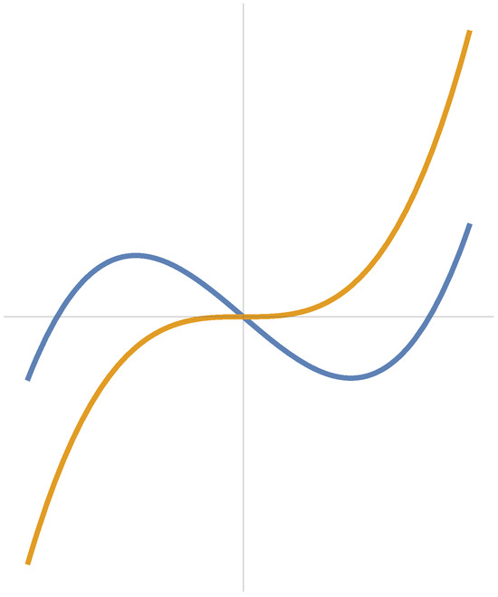
The isotropic curvature as a function of s is again given by ${\kappa }_{\mathbb{I}}\left(s\right)=s$ (see Figure 2).

Example 4.

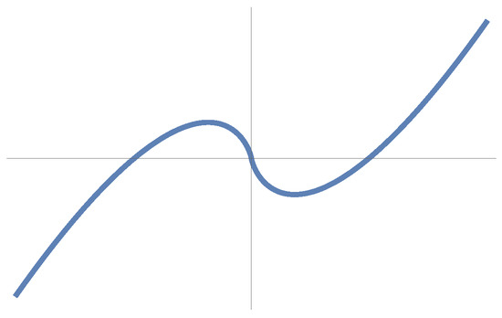
The curve with the isotropic curvature ${\kappa }_{\mathbb{I}}=\frac{1}{s}$ in ${\mathbb{I}}^2$ is a curve $c\left(s\right)=(s,s\ln |s\left|\right)$. If we choose that c lies in a lightlike plane spanned by $(0,1,0)$ and $(1,0,1)$, then c is a pseudo-null curve in ${\mathbb{M}}^3$ parametrized by

$$c\left(s\right)=s\left(\ln \right|s|,1,\ln |s\left|\right).$$

Its pseudo-torsion is calculated as $\tau =-\frac{1}{s}$, which confirms the relation (10) (see Figure 3).

References

- Sachs, H. Lehrbuch der Ebenen Isotropen Geometrie; Vieweg: Wiesbaden, Germany, 1987. [Google Scholar]
- Duggal, K.L.; Bejancu, A. Lightlike Submanifolds of Semi-Riemannian Manifolds and Applications; Kluwer Academic Publishers: Dordrecht, The Netherlands, 1996. [Google Scholar]
- Duggal, K.L.; Jin, D.H. Null Curves and Hypersurfaces of Semi-Riemannian Manifolds; World Scientific Publishing: Singapore, 2007. [Google Scholar]
- Duggal, K.L.; Sahin, B. Differential Geometry of Lightlike Submanifolds; Birkhäuser: Basel, Switzerland, 2010. [Google Scholar]
- Camci, Ç.; Uçum, A.; İlarslan, K. New results concerning Cartan null and pseudo null curves in Minkowski 3-space. J. Geom. 2023, 114, 15. [Google Scholar] [CrossRef]
- da Silva, L.C.B. Moving frames and the characterization of curves that lie on a surface. J. Geom. 2017, 108, 1091–1113. [Google Scholar] [CrossRef]
- López, R.; Milin Šipuš, Ž.; Primorac Gajčić, L.; Protrka, I. Involutes of pseudo-null curves in Lorentz–Minkowski space. Mathematics 2021, 7, 1256. [Google Scholar] [CrossRef]
- Kühnel, W. Differential Geometry: Curves-Surfaces-Manifolds; American Mathematical Society: Providence, RI, USA, 2005. [Google Scholar]
- López, R. Differential geometry of curves and surfaces in Lorentz–Minkowski space. Int. Electron. J. Geom. 2014, 7, 44–107. [Google Scholar] [CrossRef]
- Walrave, J. Curves and Surfaces in Minkowski Space. Ph.D. Thesis, K. U. Leuven, Faculteit Der Wetenschappen, Leuven, Belgium, 1995. [Google Scholar]
- Osmar, A.; Badr, S.A.-N.; Hassan, S.A.; Rodrigues, L.A.; Silva, F.N.; Soliman, M.A. Transversal Intersection Curves of Two Surfaces in Minkowski 3-Space. Sel. Mat. 2018, 5, 137–153. [Google Scholar]
- Topbas, G.I.; Ekmekci, N.; Yayli, Y. Darboux Frame of a Curve Lying on a Lightlike Surface. Math. Sci. Appl. E-Notes 2016, 4, 121–130. [Google Scholar] [CrossRef]
- Bonnor, W.B. Curves with null normals in Minkowski space–time. In A Random Walk in Relativity and Cosmology; Dadhich, N., Ed.; Wiley Easten Limited: New Delhi, India, 1985; pp. 33–47. [Google Scholar]
- Pekmen, U.; Pasali, S. Some characterizations of the Lorentzian spherical space-like curves. Math. Morav. 1999, 3, 33–37. [Google Scholar]
- Petrović-Torgašev, M.; Šućurović, E. Some characterizations of the spacelike, the timelike and the null curves on the pseudohyperbolic space H0 in . Kragujev. J. Math. 2000, 22, 78–82. [Google Scholar]
- Petrović-Torgašev, M.; Šućurović, E. Some characterizations of the Lorentzian spherical spacelike with the timelike and the null principal normals. Math. Morav. 2000, 4, 83–92. [Google Scholar] [CrossRef]
- Milin Šipuš, Ž.; Primorac Gajčić, L.; Protrka, I. Generalized helices on a lightlike cone in 3-dimensional Lorentz–Minkowski space. KoG 2020, 24, 41–46. [Google Scholar] [CrossRef]
Disclaimer/Publisher’s Note: The statements, opinions and data contained in all publications are solely those of the individual author(s) and contributor(s) and not of MDPI and/or the editor(s). MDPI and/or the editor(s) disclaim responsibility for any injury to people or property resulting from any ideas, methods, instructions or products referred to in the content. |
© 2023 by the authors. Licensee MDPI, Basel, Switzerland. This article is an open access article distributed under the terms and conditions of the Creative Commons Attribution (CC BY) license (https://creativecommons.org/licenses/by/4.0/).