Dynamic Analysis of Impulsive Differential Chaotic System and Its Application in Image Encryption

Abstract

In this paper, we study the dynamic behavior of an impulse differential chaotic system which can be applied to image encryption. Combined with the chaotic characteristics of the high dimensional impulsive differential equations, the plaintext image can be encrypted by using the traditional Henon map and diffusion sequences encryption algorithm. The initial values and control parameters serve as keys for encryption algorithms, and the algorithm has a larger key space. The key is resistant to minor interference and the accuracy can reach ${10}^{-12}$. The simulation results show that the impulsive differential chaotic system has a good application prospect in image encryption.

1. Introduction

With the development and application of the Internet, big data, and 5G networks, more and more people use mobile terminals such as smartphones to transmit media files such as images, texts, and videos. In particular, the application of the social platform APP has has generated a large amount of image transmission and storage, and the security and confidentiality of image transmission in networks has been paid more and more attention. Therefore, the image encryption algorithm has become one of the key directions of researchers’ attention [1,2,3].

Image encryption based on chaotic sequences is one of the most popular image encryption algorithms [4]. Chaos is a kind of complex dynamic behavior possessed by nonlinear dynamic systems. It is the inherent randomness of deterministic nonlinear systems. “Deterministic system” means that the mathematical model describing the system is expressed as a fully deterministic equation that does not contain any random factors. Chaotic systems can usually be divided into two categories: discrete iterative mapping and continuous systems.

At present, many safe and convenient encryption algorithms have been proposed, such as image encryption algorithms based on the Lorenz system, Chua’s system [5], logistic mapping [6,7], tent mapping [8], Henon mapping [9], and other systems. They are widely used in image encryption. But we know that these systems belong to continuous chaotic systems or discrete iterative maps. After decades of research on impulsive differential systems, it was found that impulsive differential systems have the characteristics of continuous systems and discrete systems, but they also have properties beyond the range of continuous systems and discrete systems [10,11,12]. The theoretical research on impulsive differential equations began in the 1960s. In the 1990s, after the research and efforts of many scholars, the basic theorem of the existence of impulsive differential equation solutions, impulsive differential/integral inequalities and basic theories of impulsive differential equation stability were gradually established [13,14,15].

In recent years, many researchers have introduced impulsive differential equations into population dynamics. Through research, it has been found that impulsive differential systems have complex dynamic behaviors, including quasi-periodic oscillation, double-period branching, half-period branching, periodic window, chaos [16], etc.

Based on the analysis and research of a class of impulsive differential equations, this paper proposes a chaotic image encryption algorithm based on impulsive differential chaotic systems.

2. Impulsive Differential Equations

The encryption algorithm used in this article is based on impulsive differential equations, we briefly introduce the impulsive differential equations in the next section.

2.1. Introduction to Impulsive Differential Equations

Impulsive differential equations have the characteristics of continuous systems and discrete systems. Under certain parameter conditions, complex dynamic behavior will occur. Different impulsive disturbances will fundamentally change the system. The stability and periodicity of the numerical solutions of the system change accordingly. Because of the sensitivity to the initial value, the dynamic behavior of the system is difficult to predict. The system will exhibit double-period branching, half-period branching, quasi-periodic oscillation, periodic waterfall, chaos, and other phenomena in the specific value range, so the resulting sequence is difficult to predict. Based on this, we use the chaotic characteristics of the impulsive differential equations and the sequences generated by them to perform certain processing transformations for image encryption; we can also combine Henon maps or logistics maps to take their numerical solutions as the input of the initial value of the map, and then generate a new encrypted sequence which expands the way to generate the encrypted sequence and the key space. As a result, it improves the security of the image encryption algorithm.

The impulsive differential equations used in this article are the following three-dimensional impulsive differential equations as shown in Equation (1). Equation (1) is a mathematical model of the Gompertz virus disease for pest control, with pulse effect and a Holling II functional response function.

$$\{\begin{array}{ll}\frac{dS(t)}{dt}=S(t)[r\mathit{ln}\frac{K}{S(t)+\alpha I(t)}-\beta \frac{V(t)}{1+mS(t)}],& \\ \frac{dI(t)}{dt}=\beta \frac{V(t)}{1+mS(t)}-dI(t),& t\ne nT,\\ \frac{dV(t)}{dt}=-\mu V(t)+\kappa dI(t),& \\ I\left(t^{+}\right)=I(t)+p,& t=nT.\end{array}$$

(1)

where all parameters are positive constants and S(t) represents susceptible pests, I(t) represents infected pests, V(t) represents viruses, $r$ is the intrinsic growth rate, $K$ is the environmental carrying capacity, $\alpha \ge 0$, $\beta$ represents the infection rate, $m\ge 0$, $d$ represents the mortality rate due to disease, $\mu$ represents the virus mortality constant, $\kappa$ represents the virus replication parameter, and $p$ represents the continuous release of infected pests at a constant rate.

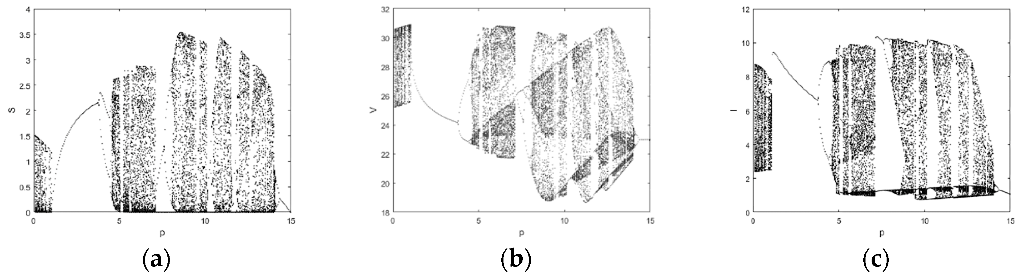
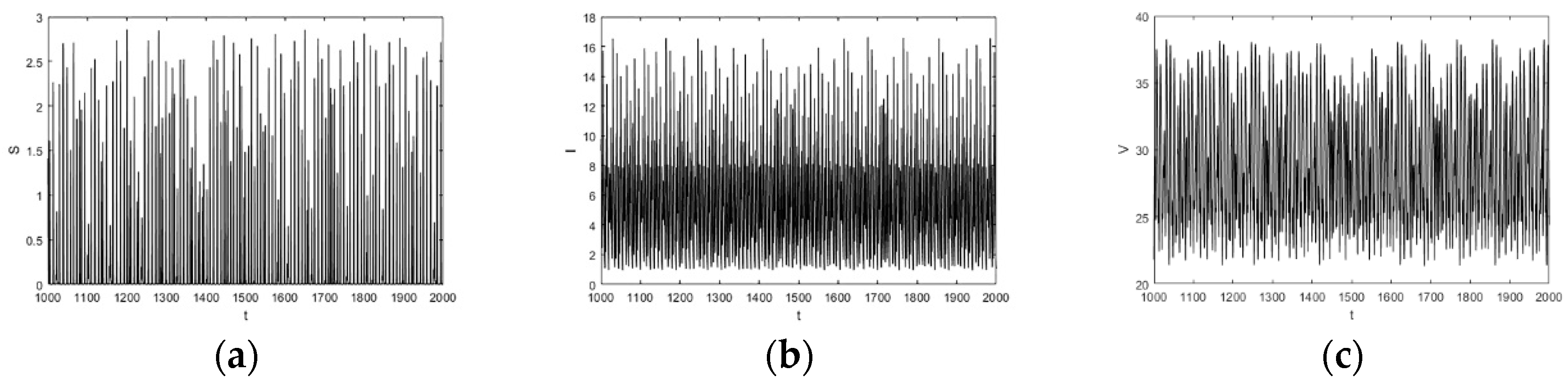
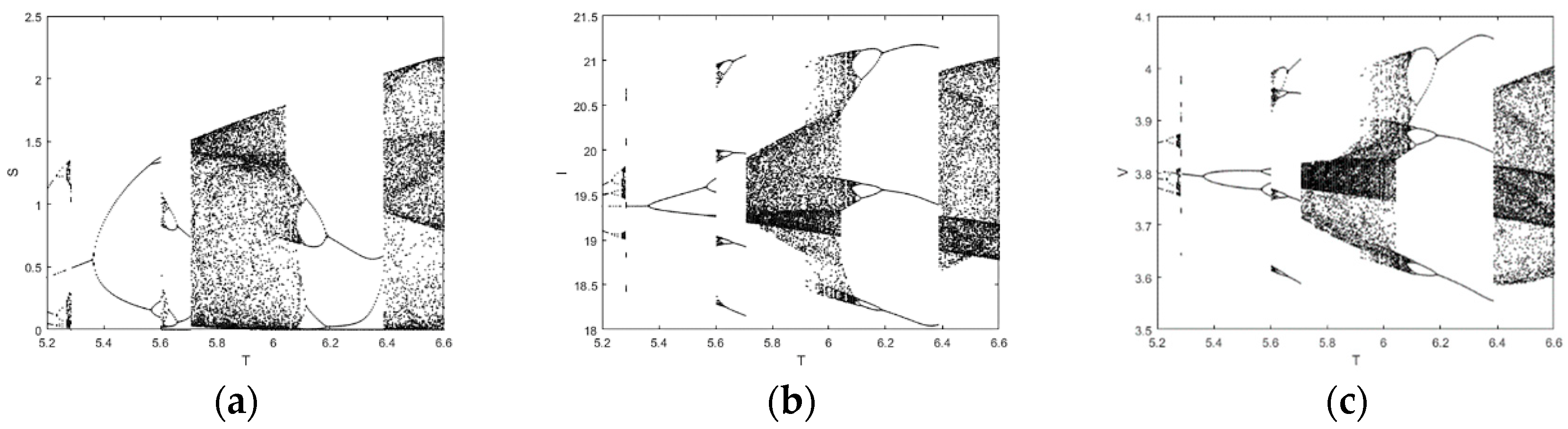
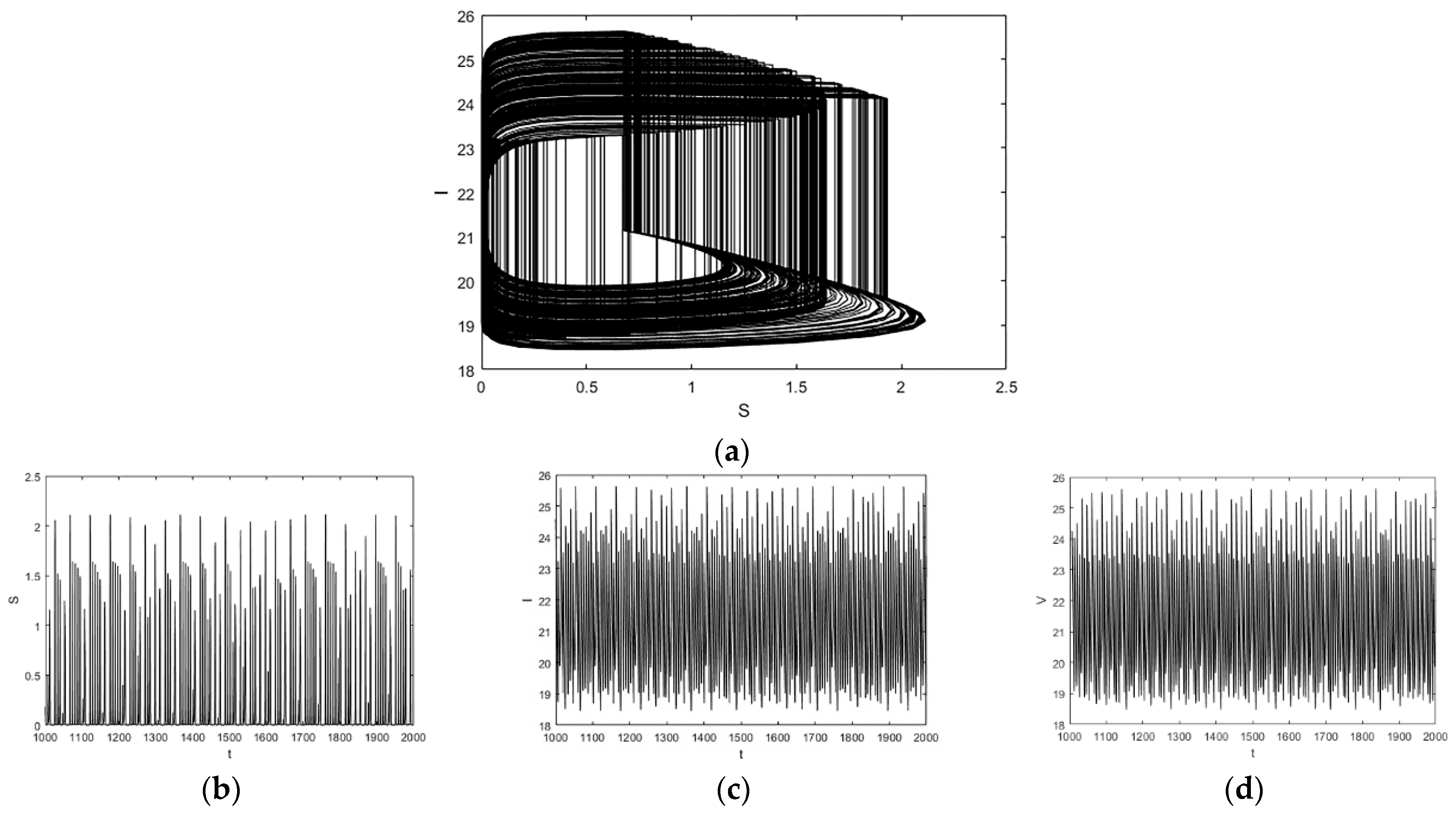
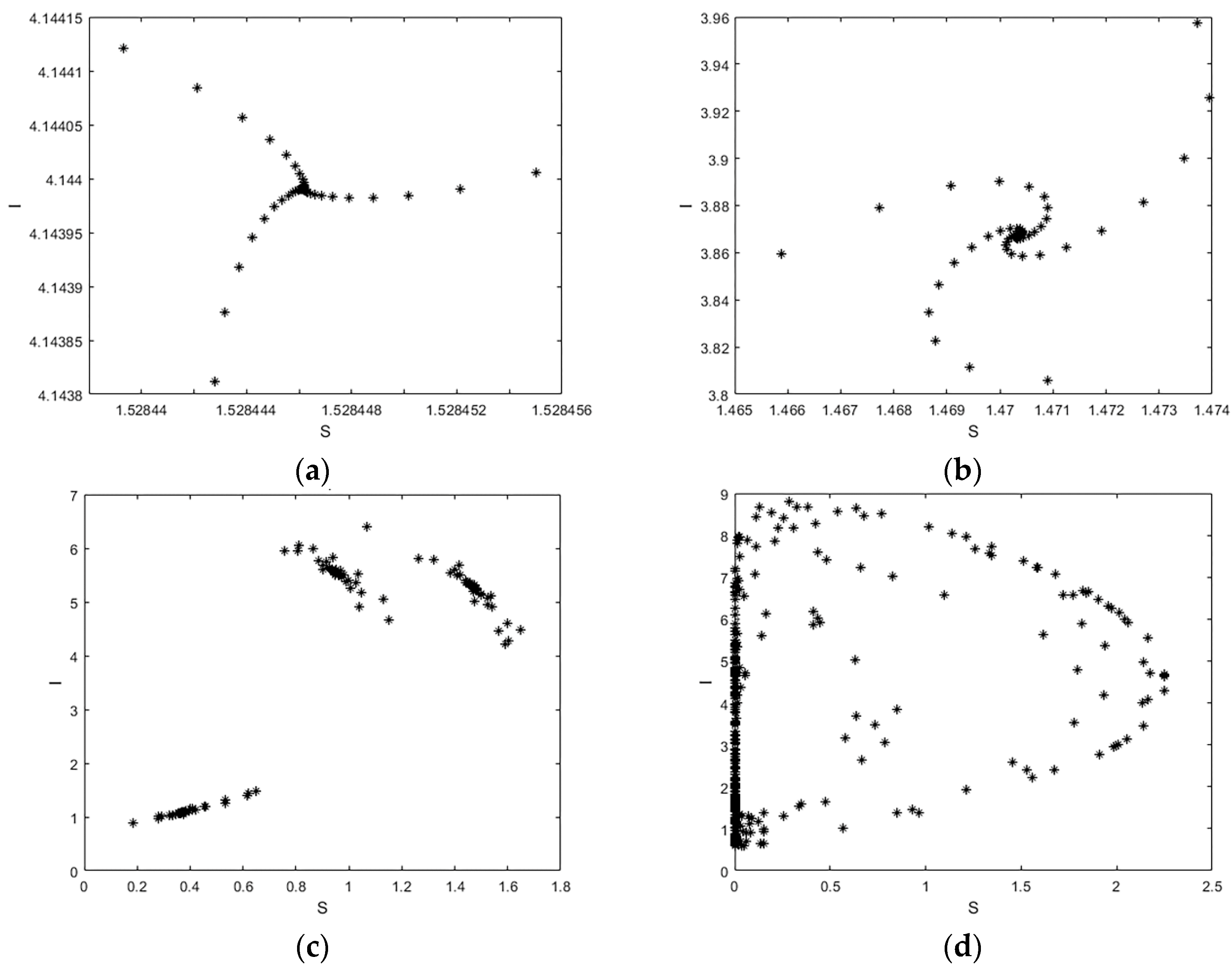
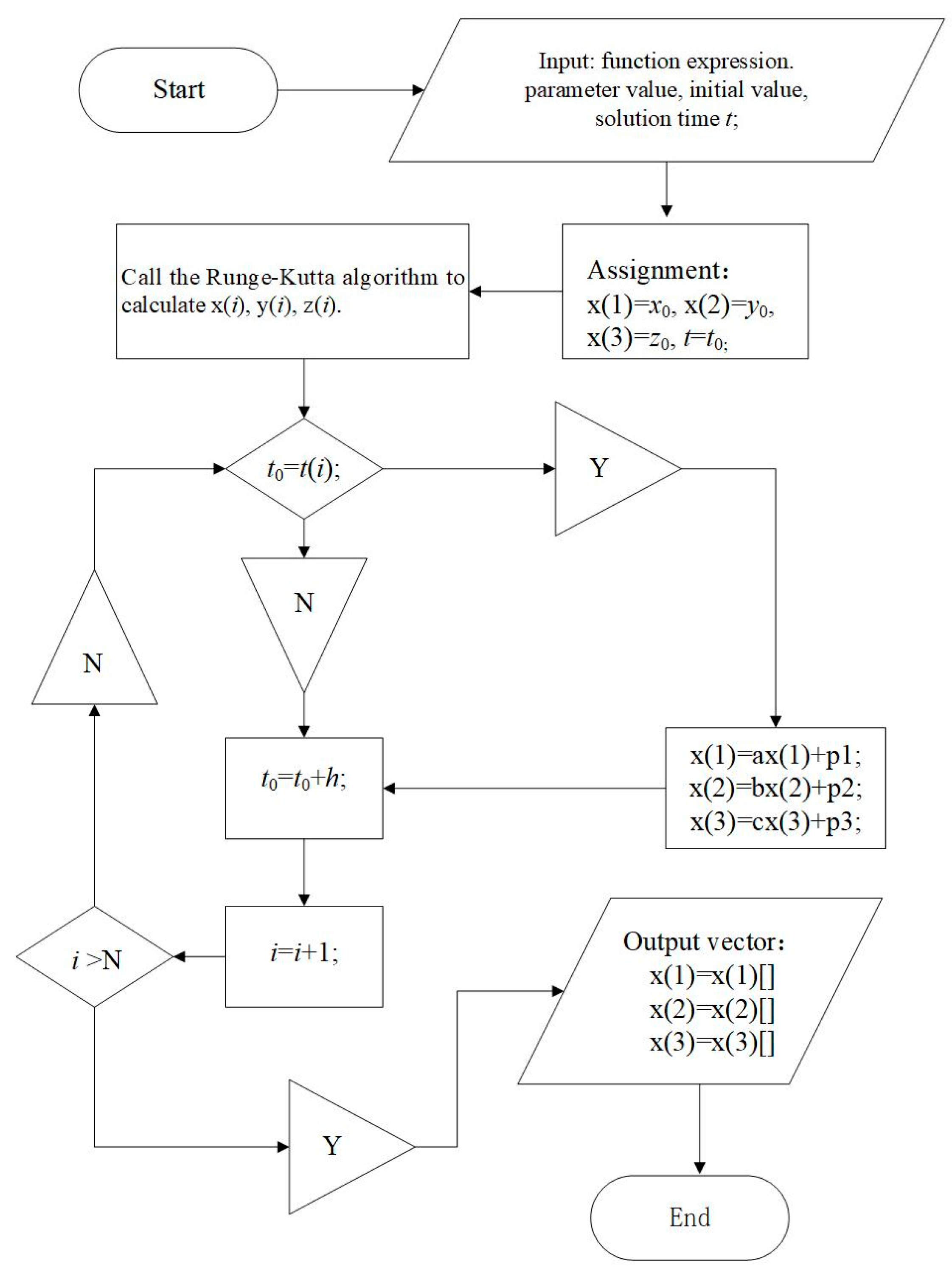
2.2. Chaotic Properties of Numerical Solutions of Impulsive Differential Equations

We use the Runge–Kutta algorithm to solve the impulsive differential equations, and the numerical simulation method can be used to visually understand the complex dynamic behavior of the equations. The following Figure 1 and Figure 2 are the bifurcation diagrams of the system under the following parameter conditions. It can be seen from the analysis of the diagram that the system has complex dynamic behaviors. With the increase of p, the system has experienced chaos → period → double period branch → chaos → period → double period branch → chaos and other dynamics, characterized by double period branch.

We can see from Figure 3, Figure 4 and Figure 5 that the period T has a very important effect on the dynamic behavior of the system. As T increases, the system undergoes a complex process: period → chaos → period → double period branch → chaos → half period branch → period → chaos. The characteristics are double-period branching and half-period branching.

Figure 6a shows a chaotic attractor of the system. The image predicts that as the parameters change, the system will undergo major changes. From Figure 7, we can see that the system has experienced complex movements.

The above are the numerical simulation results of the system. From the above figures, we can see that the system has very different dynamic behavior under different initial value conditions.

3. Design of Chaotic Image Encryption Algorithm Based on Impulsive Differential Equations

In this paper, an image encryption algorithm based on an impulsive differential system is designed by using the complex dynamic behavior of impulsive differential chaotic system, combined with the Henon map to avoid the problem of low security of a single chaotic system. The algorithm has high security, therefore, it can avoid brute force attacks and effectively protect the security of encrypted images.

3.1. Generation of Encryption Key and Encrypted Chaotic Sequence

Generally, the parameter value and initial value of the impulsive differential equation can be used as the input of the encryption key. After the parameters and initial values of the system are given, the impulsive differential equations can be solved. In this paper, the Runge–Kutta function is used to solve the system [17,18]. The flow chart of the algorithm for generating chaotic sequence of the impulsive differential equations is shown in Figure 8.

The parameters and initial values of the impulsive differential equations used in this paper are as following: Equation (2). x₀, y₀ and z₀ are the initial values of S, I, and V.

$$T=4.5;x_0=0.8;y_0=1.1;z_0=0.6;t_0=0;p=6.85;$$

(2)

In order to increase the sensitivity of the ciphertext to the plaintext, each cleartext image corresponds to a unique encryption key, and set the value of p in Equation (3):

$$p=6.85+s,$$

(3)

where s = mod(sum(sum($I$)),256)/100, I is the pixel matrix of the clear text image.

In this way, even if one pixel of the plaintext image is modified, the corresponding encryption key will also change. Through the above algorithm, three chaotic sequences x1, x2, x3 for encryption can be obtained.

Because the system may produce imaginary value solutions under different conditions, before encrypting with sequence values, we need to perform real operations on all sequence values as Equation (4):

$$x\left(i\right)=real\left(x\left(i\right)\right),$$

(4)

So that the computer can be processed.

In order to obtain a better pseudo-random sequence, we can perform mathematical processing on the generated sequence, such as performing a square root operation on each column of sequence values as Equation (5):

$$x\left(i\right)=real\left(sqrt\left(x\left(i\right)\right)\right),$$

(5)

or perform a triangle function conversion as Equation (6):

$$x\left(i\right)=real\left(\mathit{sin}\left(x\left(i\right)\right)\right), x\left(i\right)=real\left(\mathit{cos}\left(x\left(i\right)\right)\right),$$

(6)

Also, we can perform mathematical processing between two sequences, thereby greatly improving the randomness.

This article performed the following two rounds of processing in Equations (7) and (8):

$$\{\begin{array}{c}x1\left(i\right)={\left(sqrt\left(x2-sqrt\left(0.6\times x4\left(i\right)\right)\right)\right)}^3;\\ x2\left(i\right)={\left(sqrt\left(x3-sqrt\left(p\right)\times x4\left(i\right)\right)\right)}^3; \end{array}$$

(7)

$$\{\begin{array}{c}y1\left(i\right)=\left(1/3.1415926\right)\times asin\left(sqrt\left(x1\left(i\right)\right)\right); \\ y2\left(i\right)=\left(1/3.1415926\right)\times asin\left(sqrt\left(x2\left(i\right)\right)\right);\end{array}$$

(8)

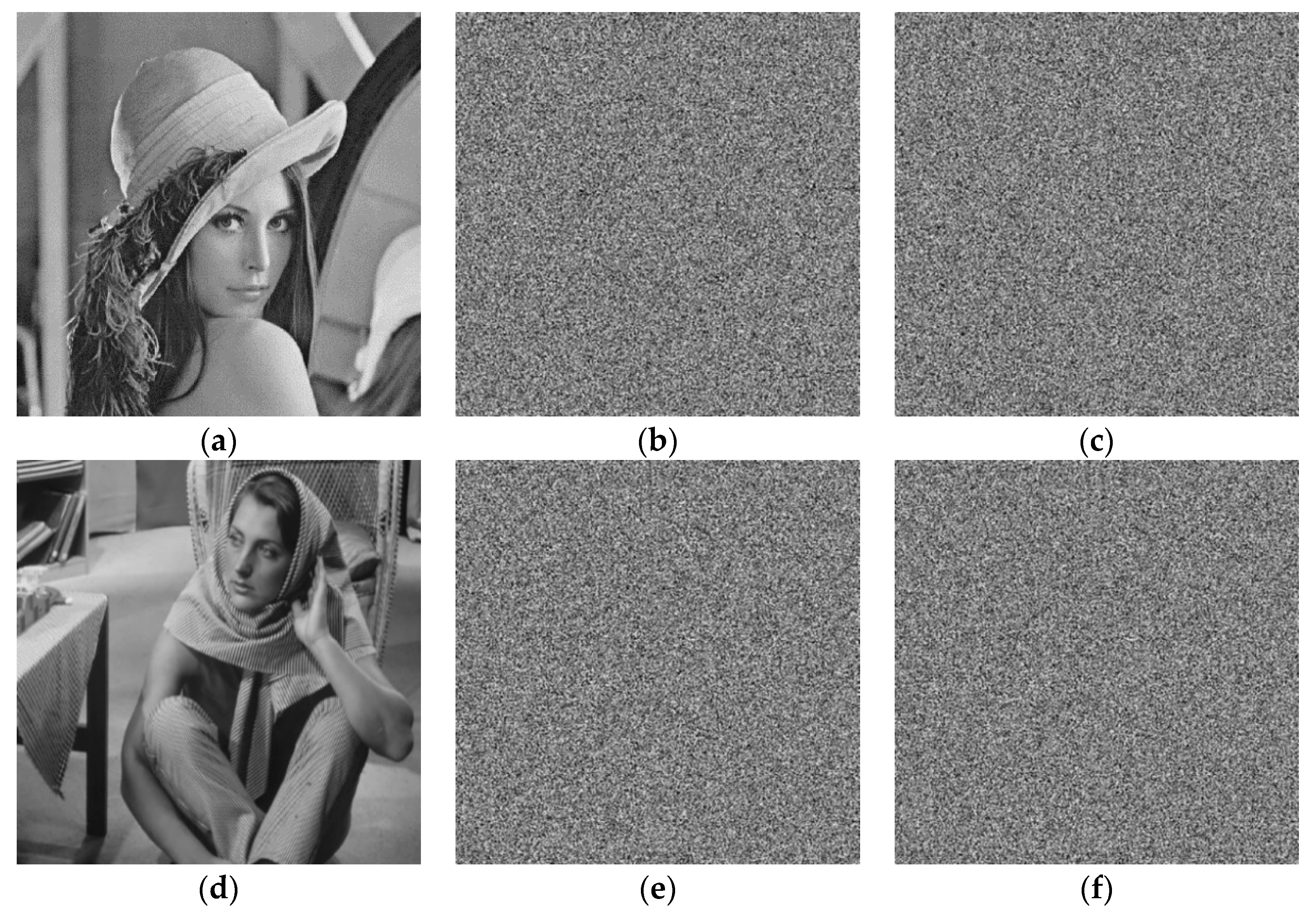
3.2. Image Encryption Process

3.2.1. Scrambling of Image Position

In order to scramble the rows and columns of the image matrix, we use the algorithm to generate chaotic sequences. Firstly, we use the Henon algorithm to scramble the plaintext image, and then use the above encryption sequences to perform pixel value replacement operations. Then, we can obtain the ciphertext image. The partial encryption pseudocode is as follows. It should be noted that some symbols in the previous and subsequent steps are same, but they do not indicate the same operation result.

To generate three chaotic sequences (xi (i = 1, 2, 3)), we run the algorithm in 3.1. Then, we can obtain four chaotic sequences (xi (i = 1, 2, 3, 4)) by performing the following processing operations:

Step1: $x1=x1\left(Nt:end\right);xi1=xi\left(Nt:end\right);\left(i=2,3\right);x41=x21-x31;$

where, xi (Nt: end) is a sufficiently chaotic sequence after discarding the sequence values of the previous Nt-1 iterations. The Nt selected in this paper is 14,000.

Then perform the following processing operations:

Step2: $x11={\left(sqrt\left(x21-sqrt\left(b\times x41\right)\right)\right)}^3;x21={\left(sqrt\left(x31-sqrt\left(b\times x41\right)\right)\right)}^3;x31={\left(sqrt\left(x1-sqrt\left(p\right)\times x41\right)\right)}^3;x41={\left(sqrt\left(x21-sqrt\left(p\right)\times x31\right)\right)}^3;xi=xi{1}^{\prime };i=1,2,3,4;$

where b = 0.6, this value can be chosen arbitrarily, the sqrt function can also be replaced with other mathematical functions. The above-mentioned processing can make the connection between each sequence closer. In this way, we have obtained four chaotic sequences x1, x2, x3, x4.

Next, we use the Henon mapping algorithm to scramble plaintext image. Assuming the size of the plaintext image to be encrypted is $L=M\times N$, the pixel matrix of the read plaintext image is denoted as I in Equation (9):

$$I=\left[\begin{array}{ccc}I\left(1\right)& I\left(2\right)& \begin{array}{cc}\cdots & I\left(N\right)\end{array}\\ I\left(N+1\right)& I\left(N+2\right)& \begin{array}{cc}\cdots & I\left(2N\right)\end{array}\\ \begin{array}{c}⋮\\ I\left(\left(M-1\right)N+1\right)\end{array}& \begin{array}{c}⋮\\ I\left(\left(M-1\right)N+2\right)\end{array}& \begin{array}{c}\begin{array}{cc}⋮& ⋮\end{array}\\ \begin{array}{cc}\cdots & I\left(L\right)\end{array}\end{array}\end{array}\right]$$

(9)

Since chaotic systems are highly sensitive to initial values and parameters, we used the following Henon map Equation (10):

$$\{\begin{array}{c}{x}_{n+1}=1-a{x}_n^2+y_n\\ y_{n+1}=b{x}_n\end{array}$$

(10)

where a = 1.4, b = 0.3. generating chaotic sequences x (n), y (n), and arranged in ascending order. The position of the sorted sequence is recorded using the corresponding position matrix $Lxy$, and the pixel position of the image I is replaced to obtain the scrambled image ${I^{\prime }}^{’}$. such as Equation (11)

$$Lxy=\left[\begin{array}{cccc}5& 7& 13& 10\\ 9& 3& 2& 15\\ 1& 4& 8& 11\\ 12& 16& 6& 14\end{array}\right]$$

(11)

Then the scrambled ${I^{\prime }}^{’}$ as following Equation (12):

$${I^{\prime }}^{’}=\left[\begin{array}{cccc}I\left(2\right)& I\left(10\right)& I\left(4\right)& I\left(7\right)\\ I\left(3\right)& I\left(9\right)& I\left(5\right)& I\left(12\right)\\ I\left(1\right)& I\left(13\right)& I\left(14\right)& I\left(11\right)\\ I\left(15\right)& I\left(16\right)& I\left(6\right)& I\left(8\right)\end{array}\right]$$

(12)

3.2.2. Pixel Value Diffusion Replacement

After obtaining the scrambled image, we use the new chaotic system to generate chaotic sequences to improve the encryption effect, and perform the first round of diffusion operation on the scrambled image.

For the four chaotic sequences obtained from step1 and step2, we proceed as follows to obtain two chaotic sequences x1, x2 for encryption:

Step3: $xi\left(n\right)=\left(\frac{1}{pi}\right)\times asin\left(sqrt\left(xi\left(n\right)\right)\right)\left(i=1,2;n=M\times N\right);$

$ki\left(n\right)=mod\left(floor\left(real\left(xi\left(n\right)\right)\times {10}^{15}\right),256\right)\left(i=1,2;n=M\times N\right);$

where floor means rounding down, real means taking the value of the real part, $ki\left(n\right)\in \left[0, 255\right]$;

Then perform XOR operation on the scrambled image pixels:

Step4:

if $mod\left(n,1\right)==0$

$k\left(n\right)=k1\left(n\right);$

  else $k\left(n\right)=k2\left(n\right);$

$Ac\left(i,j\right)=bitxor\left(I^{\prime }\left(i,j\right),k\left(n\right)\right);$

Afterwards, we use the remaining two chaotic sequences x3, x4 to perform the second round of diffusion operation on the encrypted ciphertext image:

Step5:

$xi\left(n\right)=\left(\frac{1}{pi}\right)\times asin\left(sqrt\left(xi\left(n\right)\right)\right),\left(i=3,4;n=M\times N\right)$;

$ki\left(n\right)=mod\left(floor\left(real\left(xi\left(n\right)\right)\times {10}^{14}\right),256\right),\left(i=3,4;n=M\times N\right);$

if $mod\left(n,2\right)==0$

$k\left(n\right)=k3\left(n\right);$

else

$k\left(n\right)=k4\left(n\right);$

$Ac\left(i,j\right)=bitxor\left(Ac\left(i,j\right),k\left(n\right)\right);$

where $Ac\left(i,j\right)$ is an intermediate variable.

Finally, the encrypted image pixel sequence is converted into an $M\times N$ matrix to obtain the final ciphertext image C.

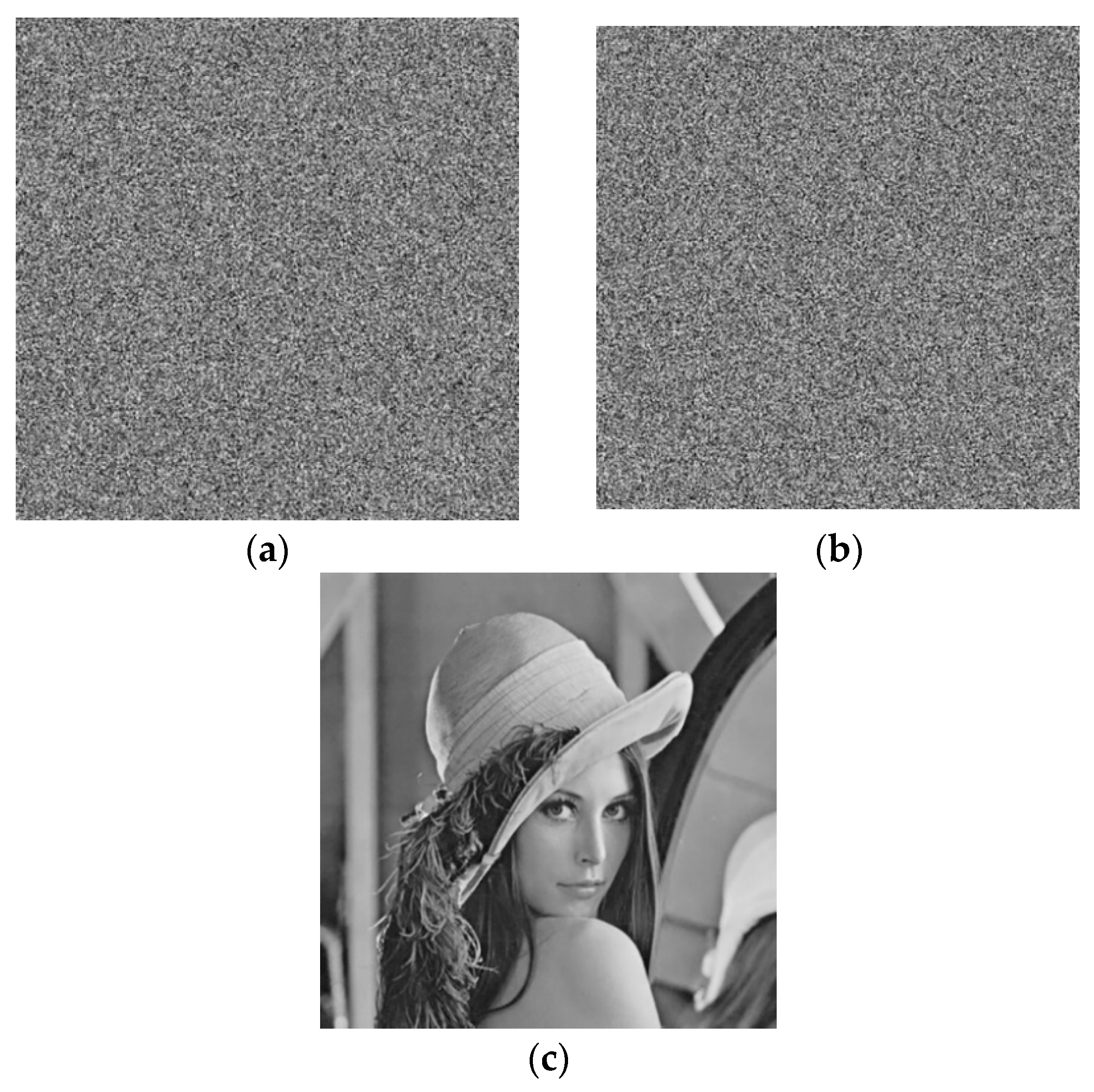
3.3. Image Decryption

The decryption process of the cipher text image is similar to the encryption process. If the reverse operation is performed, the decrypted image can be obtained. It will not be repeated here.

4. Results and Safety Analysis

The performance of the actual execution time of each scheme depends on many factors such as number of iterations, programming method, and coding efficiency, as well as platform specifications. In this paper, we performed image encryption on Lena, Peppers, Barbara, and Girl. The average time consumed to encrypt a $512\times 512$ image was 0.730 s.

4.1. Key Sensitivity Test

In order to verify the effectiveness and feasibility of the algorithm, we performed simulation experiments using scientific computing software such as Matlab 2014b. Figure 9 shows the plain text image and the cipher text image.

In order to test the sensitivity of the key, we only modified the initial encryption key T = 4.5 to obtain the following two error decryption keys T = 4.5 + ${10}^{-10}$ and T = 4.5 + ${10}^{-12}$. Then, used incorrect keys and the correct key to decrypt the ciphertext image. Finally, we received the following error decrypted images and correctly decrypted image in Figure 10.

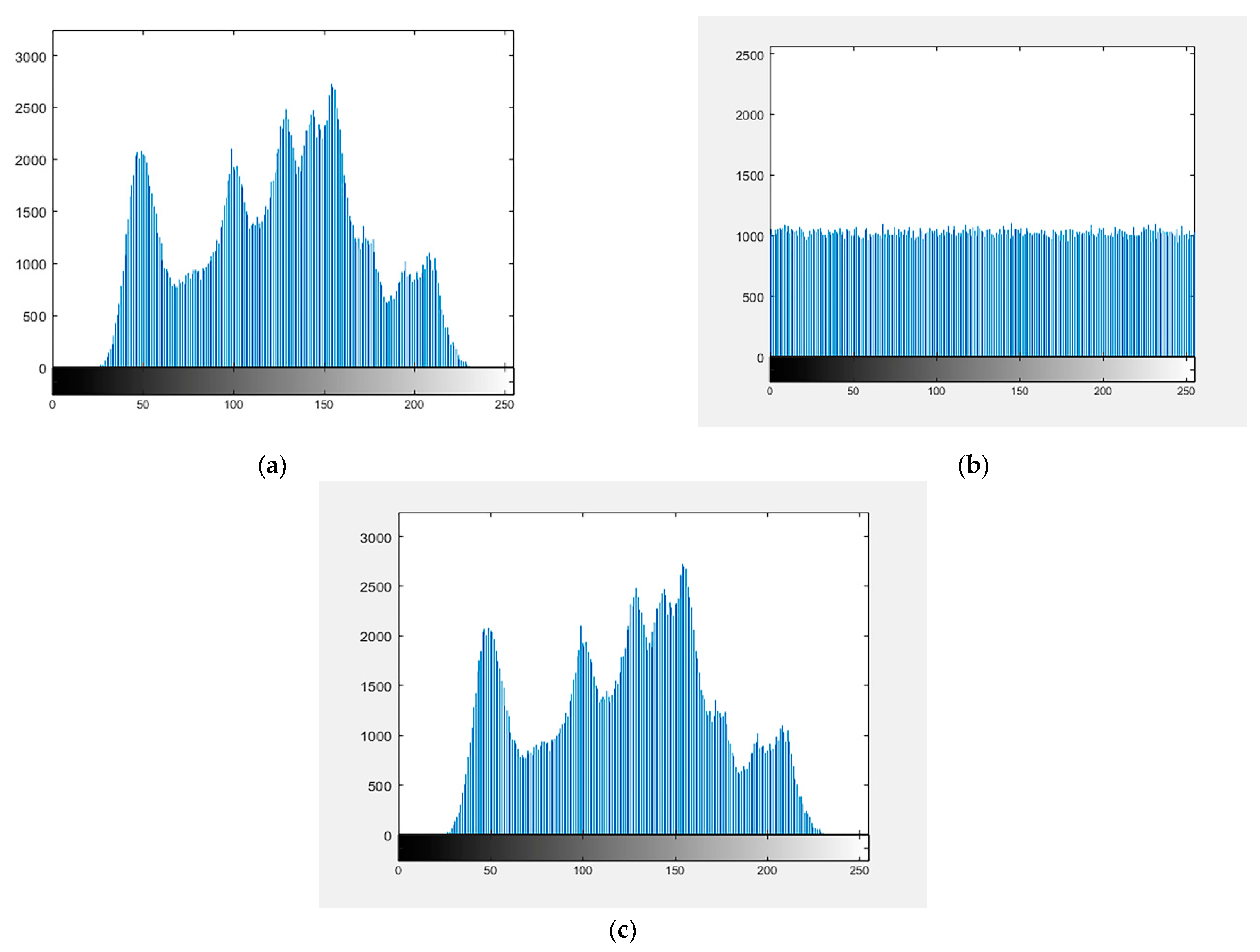
4.2. Histogram Analysis

Figure 11 shows the histograms of the plaintext image, ciphertext image and the decrypted image. We can see that after the plain text image is encrypted, the image information has changed, and the attacker cannot obtain the relevant plaintext image information, thereby protecting the encrypted information from direct cracking.

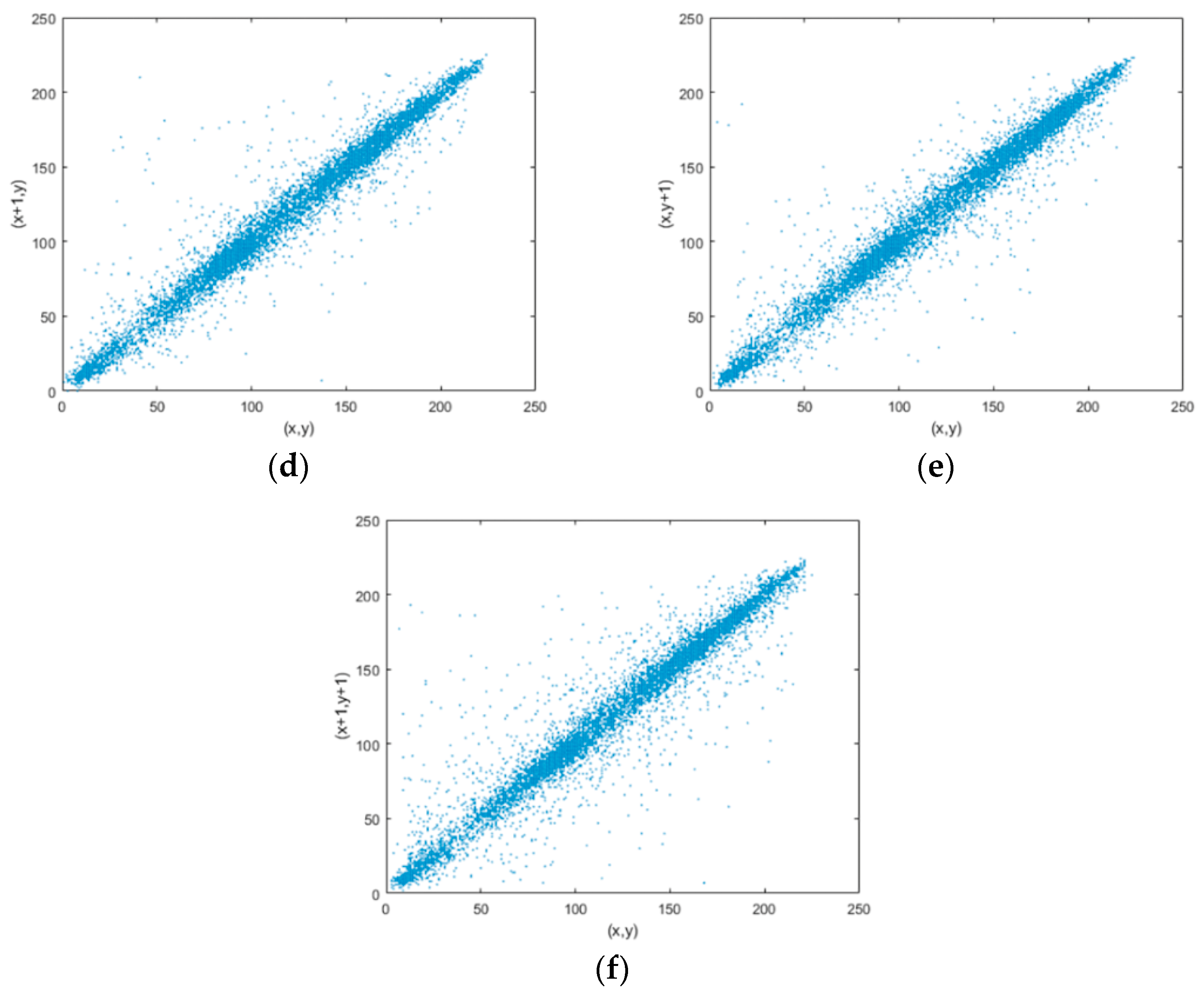
4.3. Correlation Analysis of Adjacent Pixels

Correlation reflects the relationship between the adjacent pixels of an image. In a meaningful image, the adjacent pixels are usually relatively close. As we all know, an effective image encryption should make the adjacent pixels of the encrypted image not so close. Correlation analysis can effectively judge the performance of the encryption algorithm. N pairs of pixel values are randomly selected from the plaintext image and the ciphertext image, then, we calculate the correlation coefficients in the horizontal, vertical, and diagonal directions according to the Equations (13)–(16) [19]. The result of correlation analysis of plaintext images is shown in Figure 12, and result of ciphertext images is shown in Figure 13. We can find that correlation between the adjacent pixels in plaintext images is high, and it becomes low in ciphertext images from

Table 1. Correlation coefficients of adjacent pixels of plain text images and cipher text images.

Test Image	Horizontal	Vertical	Diagonal
Lena’ Plaintext image	0.9848	0.9702	0.9587
Lena’ Ciphertext image	0.0020	0.0131	0.0070
Peppers’ Plaintext image	0.9802	0.9799	0.9669
Peppers’ Ciphertext image	0.0042	0.0160	0.0027
Ref. [20]	0.0118	0.0002	0.0148
Ref. [21]	−0.475	0.196	0.135
Ref. [22]	0.0029	−0.0342	−0.0021

. Compared with the Refs. [20,21], the correlation coefficients of the proposed algorithm in three directions are very close to their values. So, the proposed algorithm has a high security.

$$cov\left(x,y\right)=E\left\{\left(x-E\left(x\right)\right)\left(y-E\left(y\right)\right)\right\},$$

(13)

$$r_{xy}=\frac{cov\left(x,y\right)}{\sqrt{D\left(x\right)}\sqrt{D\left(y\right)}},$$

(14)

where

$$E\left(x\right)=\frac{1}{N}{\sum }_{i=1}^N{x}_i,$$

(15)

$$D\left(x\right)=\frac{1}{N}{\sum }_{i=1}^N{\left(x_i-E\left(x\right)\right)}^2.$$

(16)

4.4. Key Space Analysis

A good algorithm should have a large key space to resist the brute force attack. If the operational precision of the computer is ${10}^{-14}$ and parameters of the functions are used as encryption keys, the size of key space will be ${10}^{14}\times {10}^{14}\times {10}^{14}\times {10}^{14}\times {10}^{14}\times {10}^{14}\dots \times {10}^{14}={10}^{224}$. The result shows that the key space is very large. The general exhaustive cracking attack is almost impossible to make work, making the security of the ciphertext is guaranteed.

4.5. Information Entropy Analysis

Entropy refers to the degree of chaos in a system and it has important applications in the fields of cybernetics, probability theory, number theory, astrophysics, and life sciences. Claude E. Shannon introduced the concept of entropy to information theory for the first time. Image information entropy is a statistical form of image features, which reflects the average amount of information in an image. The more confusing the image information, the greater the information entropy and the closer to the ideal value [20,23]. The definition [23] of information entropy is:

$$H\left(m\right)={\sum }_{i=0}^{2^N-1}p\left(m_i\right){\mathit{log}}_2\frac{1}{p\left(m_i\right)},$$

(17)

where $m$ is the information source, N represents the number of bits of $m_i$, and $p\left(m_i\right)$ represents the appearing probability of $m_i$.

According to the above Equation (17), we can calculate the information entropy of the Lena image and Peppers image before and after encryption. The results of the encrypted image information entropy are listed in

Table 2. Information entropy of ciphertext images.

Test Image	Information Entropy of Ciphertext Images
Lena(512 $\times$512)	7.9686
Peppers(512 512)	7.9681
Baboon(512 $\times$512)	7.9675
Barbara(512 $\times$512)	7.9687
Ref. [22]	7.9485
Ref. [23]	7.9993
Ref. [24]	7.9994

. The table also lists the information entropy applying other algorithms to encrypt Lena images.

The information entropy of the Lena plaintext image is 7.4455, the information entropy of the Lena ciphertext image is 7.9686, the information entropy of the Pepper plaintext image is 7.5922, and the information entropy of the Pepper ciphertext image is 7.9681. We can see that the values are very close to 8. Because the value distribution is very uniform, it is difficult to find the crack information from the ciphertext image.

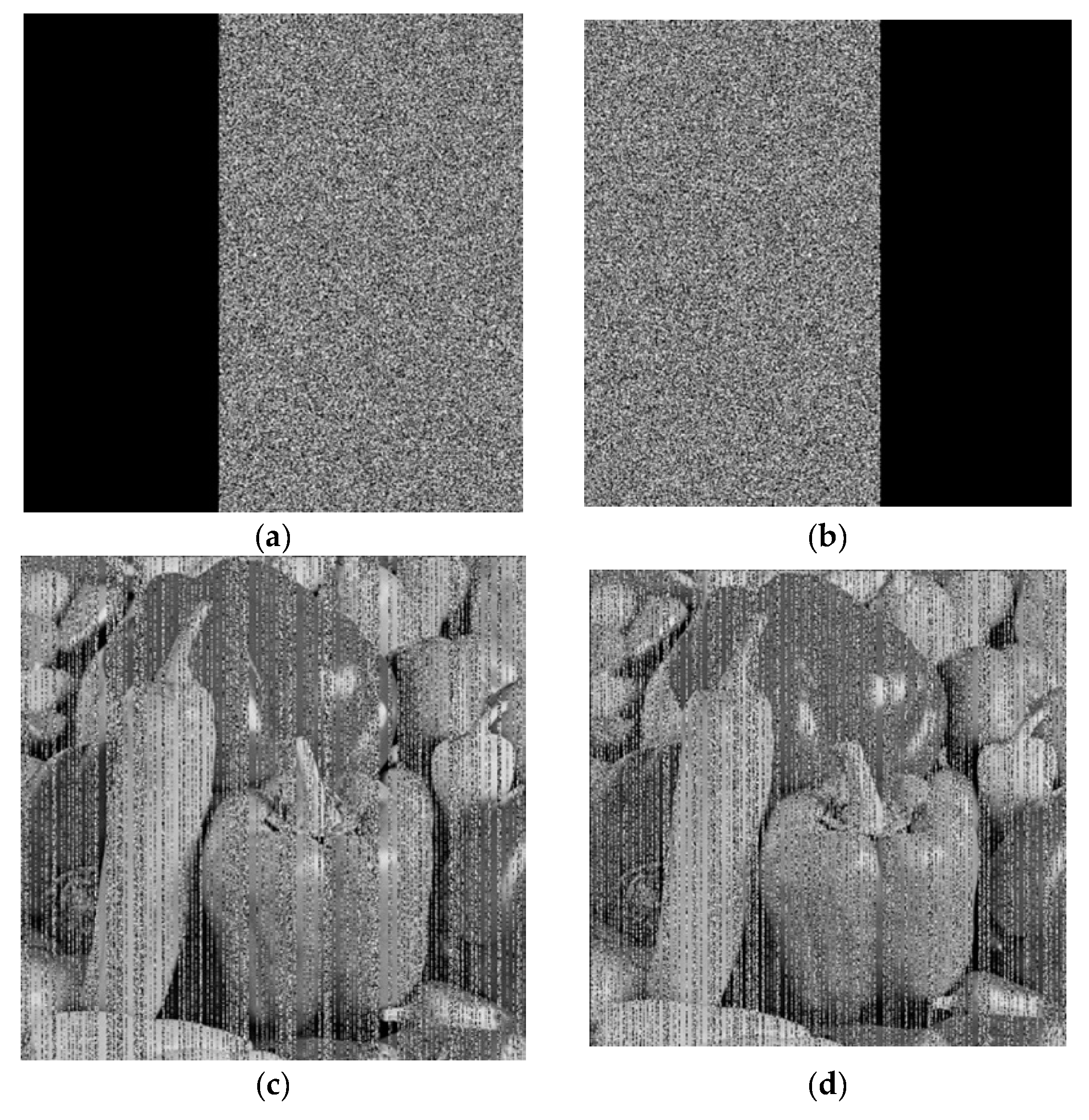
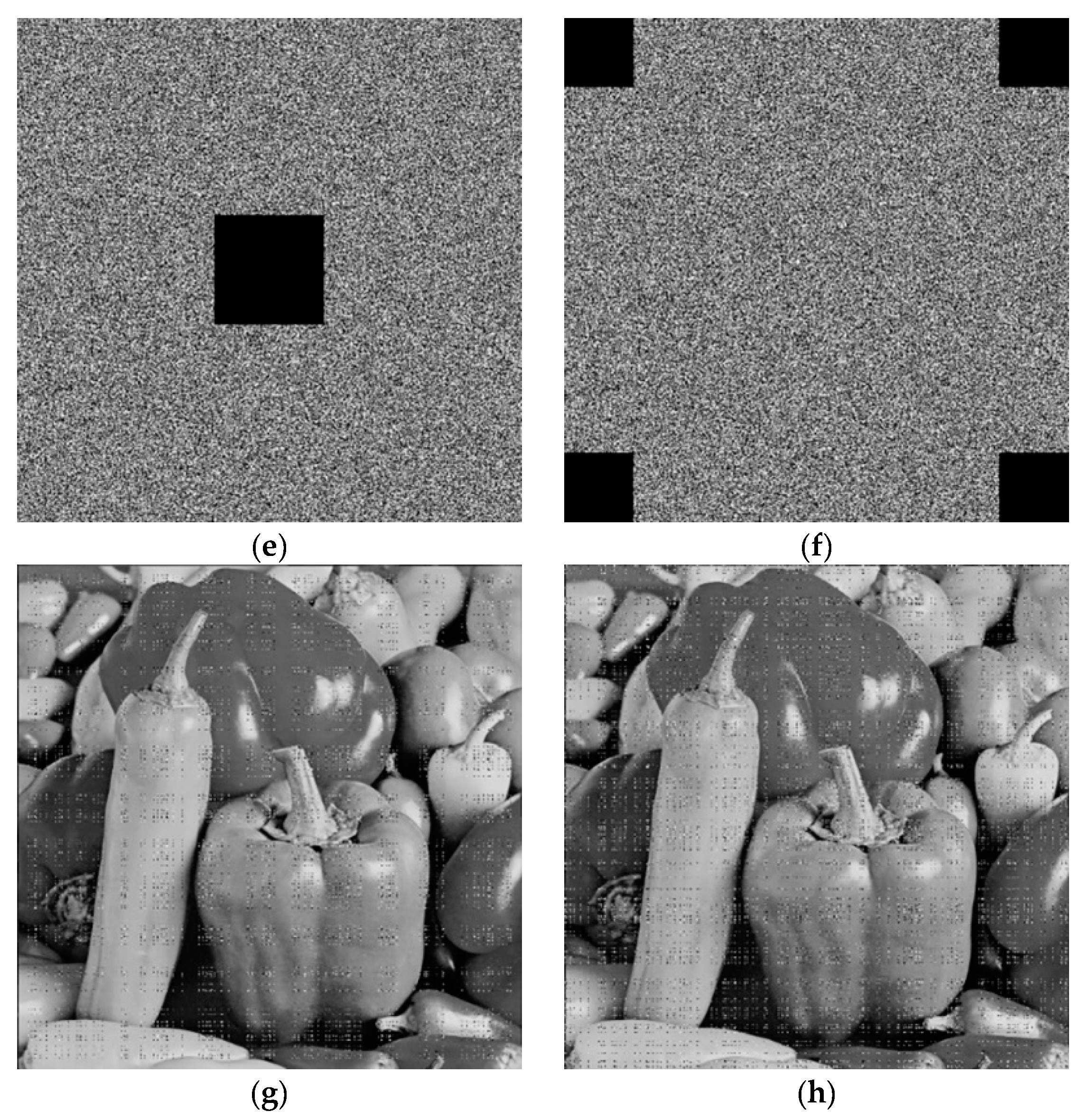
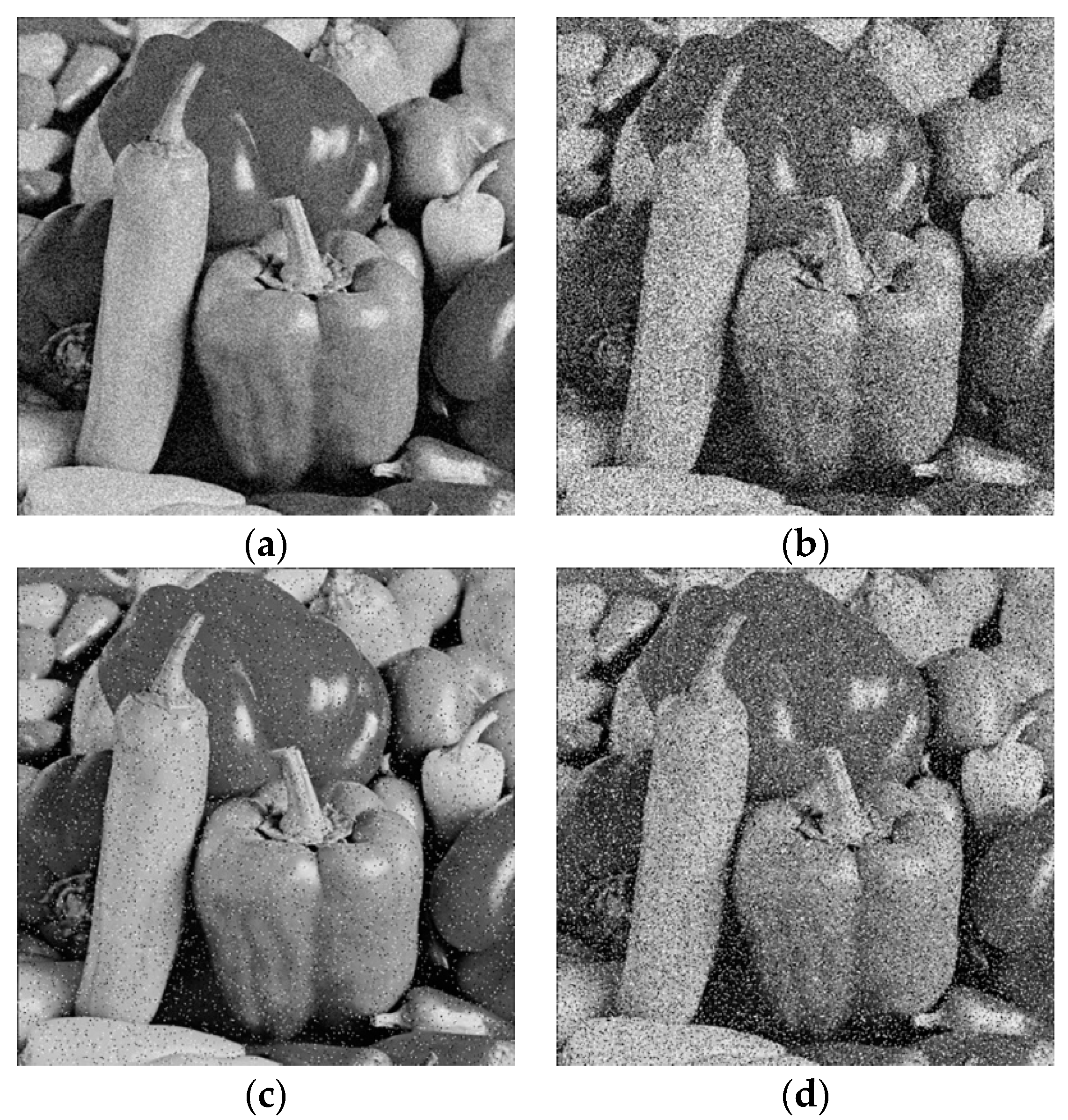
4.6. Anti-Shear and Noise Attack Analysis

The ability to withstand an attack reflects the security of the image encryption algorithm [21,25,26]. Figure 14 is the result of the shear attack test. Four kinds of shear methods are selected respectively. The test results show that the algorithm can withstand the shear attack well and the algorithm has high security.

The result of the noise attack test is shown in Figure 15. We conducted a Gaussian noise attack and a salt and pepper noise attack. The test results show that the algorithm can withstand the noise attack well [23,25]. It shows that the Gompertz virus disease mathematical model can not only provide high-quality chaotic sequences, but also provide more key space. And, the keys are resistant to small changes and have an extremely high sensitivity.

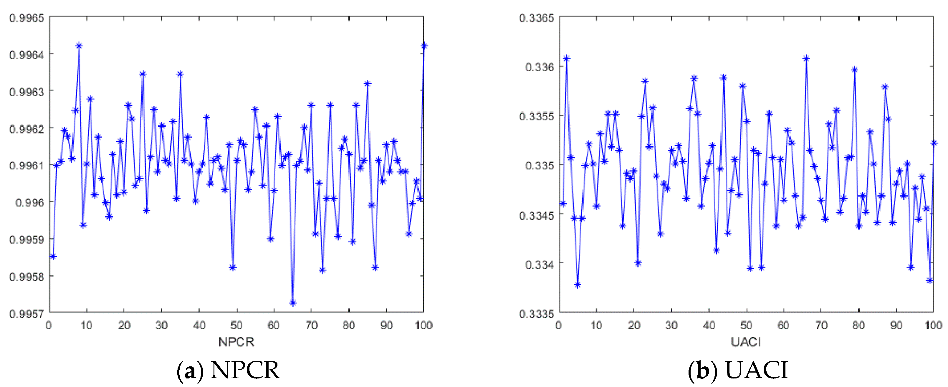
4.7. NCPR and UACI Analysis

In order to test the effect of a pixel change in the plaintext image on the overall encryption result of the algorithm, two common measures are adopted: pixel change rate (NPCR) and uniform average change degree (UACI). If pixel value changes cause the ciphertext image significant changes, it indicates that the algorithm can resist differential attacks. As we all know, the theoretical expected value of NPCR is 99.6094%, and the expected value of UACI is 33.4635% [27,28].

$$NPCR=\frac{1}{M\times N}{\sum }_{i=1}^M{\sum }_{j=1}^{N}D\left(i,j\right)\times 100\%,$$

(18)

$$UACI=\frac{1}{M\times N}{\sum }_{i=1}^M{\sum }_{j=1}^N\frac{\left|D_1\left(i,j\right)-D_2\left(i,j\right)\right|}{255}\times 100\%.$$

(19)

where $D_1$ is the ciphertext image, and $D_2$ is the ciphertext image encrypted after the pixel value of the plaintext image changes.

Here, we changed the pixels of the Lena plaintext image 100 times, randomly changing five pixels at a time to simulate a differential attack. The attack test results are shown in Figure 16, and the average value of the attack results is calculated as follows:

$$mean\_NCPR=0.996099662780762,$$

$$mean\_UACI=0.334936298594755,$$

The average values of 100 NPCR and UACI values are 99.60997% and 33.49363%, respectively, which are very close to the theoretical expected values of NPCR and UACI of 8-bit grayscale images, 99.6094% and 33.4635%. It can be said that the algorithm has a good effect against differential attacks.

5. Conclusions

In the field of image encryption, there have been many examples of chaotic systems being applied [29,30]. These examples can be roughly divided into two types: one is to directly use the existing classical chaos mapping or combine the classic chaos mapping with other algorithms [31,32,33]; the other is to improve the original classical chaos mapping based on it, and then apply image encryption [34,35]. A major difference in this article is the search for new chaotic systems. Through our efforts, we found that there is a chaotic system with pulse control in the predator-prey system. Based on this, we conducted detailed research and applied this new chaotic system to image encryption.

Based on the above, we know that impulsive differential chaotic systems have complex dynamic behavior, which can be applied to image encryption. Generally, image encryption schemes use discrete iterative mapping or continuous systems [29]. The image encryption scheme based on the impulsive differential chaotic system proposed in this paper uses the impulsive differential equations, combined with the traditional Henon encryption algorithm to encrypt plaintext images. The security of encryption is high. Because the system is high dimensional, initial values and parameters can also be used as keys, the algorithm has a large key space [25,29]. In the encryption process, the chaotic sequence is used to achieve pixel scrambling, and the three rounds of diffusion operation also make the statistical characteristics of the ciphertext image meet the higher encryption requirements. Based on the above, the proposed algorithm in this paper has a high security. In order to improve the security of encryption, we need to further study impulsive differential chaotic systems and improve the algorithm.

References

1. Wan, Y.J.; Wang, S.M.; Du, B.X. A bit plane image encryption algorithm based on compound chaos. Multimed. Tools Appl. 2023, 82, 22103–22121. [Google Scholar] [CrossRef]
2. Pourasad, Y.; Ranjbarzadeh, R.; Mardani, A. A New Algorithm for Digital Image Encryption Based on Chaos Theory. Entropy 2021, 23, 341. [Google Scholar] [CrossRef] [PubMed]
3. Chen, Y.; Tang, C.; Ye, R. Cryptanalysis and improvement of medical image encryption using high-speed scrambling and pixel adaptive diffusion. Signal Process 2020, 167, 107286. [Google Scholar] [CrossRef]
4. Yousif, S.F.; Abboud, A.J.; Alhumaima, R.S. A new image encryption based on bit replacing, chaos and DNA coding techniques. Multimed. Tools Appl. 2022, 81, 27453–27493. [Google Scholar] [CrossRef]
5. Ye, X.; Wang, X.; Gao, S.; Mou, J.; Wang, Z. A new random diffusion algorithm based on the multi-scroll Chua’s chaotic circuit system. Opt. Lasers Eng. 2020, 127, 105905. [Google Scholar] [CrossRef]
6. Sharma, M. Image encryption based on a new 2D logistic adjusted logistic map. Multimed. Tools Appl. 2020, 79, 355–374. [Google Scholar] [CrossRef]
7. Liansheng, S.; Cong, D.; Xiao, Z.; Ailing, T.; Anand, A. Double-image encryption based on interference and logistic map under the framework of double random phase encoding. Opt. Lasers Eng. 2019, 122, 113–122. [Google Scholar] [CrossRef]
8. Qumsieh, R.; Farajallah, M.; Hamamreh, R. Joint block and stream cipher based on a modified skew tent map. Multimed. Tools Appl. 2019, 78, 33527–33547. [Google Scholar] [CrossRef]
9. Luo, H.; Ge, B. Image encryption based on Henon chaotic system with nonlinear term. Multimed. Tools Appl. 2019, 78, 34323–34352. [Google Scholar] [CrossRef]
10. Holling, S.C. The Functional Response of Predators to Prey Density and its Role in Mimicry and Population Regulation. Mem. Entomol. Soc. Can. 1965, 97, 5–60. [Google Scholar] [CrossRef]
11. Pavlova, O.N.; Pavlov, A.N. Prediction of complex oscillations in the dynamics of coupled chaotic systems using transients. Phys. A Stat. Mech. Its Appl. 2020, 545, 123818. [Google Scholar] [CrossRef]
12. Bashkirtseva, I.; Ryashko, L.; Ryazanova, T. Analysis of regular and chaotic dynamics in a stochastic eco-epidemiological model. Chaos Solitons Fractals 2020, 131, 109549. [Google Scholar] [CrossRef]
13. Sugie, J. Interval oscillation criteria for second-order linear differential equations with impulsive effects. J. Math. Anal. Appl. 2019, 479, 621–642. [Google Scholar] [CrossRef]
14. Huang, C.; Yang, X.; Cao, J. Stability analysis of Nicholson’s blowflies equation with two different delays. Math. Comput. Simul. 2020, 171, 201–206. [Google Scholar] [CrossRef]
15. Fa, K.S. A class of nonlinear Langevin equation with the drift and diffusion coefficients separable in time and space driven by different noises. Phys. A Stat. Mech. Its Appl. 2020, 545, 123334. [Google Scholar] [CrossRef]
16. Pang, G.; Chen, L. Complexity of an ivlev’s predator-prey model with pulse. Adv. Complex Syst. 2007, 10, 217–231. [Google Scholar] [CrossRef]
17. Sim, C.; Sun, C.; Yun, N. A nearly analytic symplectic partitioned Runge-Kutta method based on a locally one—Dimensional technique for solving two-dimensional acoustic wave equations. Geophys. Prospect. 2020, 68, 1253–1269. [Google Scholar] [CrossRef]
18. Rathinasamy, A.; Ahmadian, D.; Nair, P. Second-order balanced stochastic Runge-Kutta methods with multi-dimensional studies. J. Comput. Appl. Math. 2020, 377, 112890. [Google Scholar] [CrossRef]
19. Liao, X.; Lai, S.; Zhou, Q. A novel image encryption algorithm based on self-adaptive wave transmission. Signal Process 2010, 90, 2714–2722. [Google Scholar] [CrossRef]
20. Alawida, M.; Teh, J.S.; Samsudin, A.; Alshoura, W.H. An image encryption scheme based on hybridizing digital chaos and finite state machine. Signal Process 2019, 164, 249–266. [Google Scholar] [CrossRef]
21. Degadwala, S.D.; Kulkarni, M.; Vyas, D.; Mahajan, A. Novel Image Watermarking Approach against Noise and RST Attacks. Procedia Comput. Sci. 2020, 167, 213–223. [Google Scholar] [CrossRef]
22. Wu, Q.; Wang, G.Y.; Jin, P.P. A improved logistic chaotic map and its application to image encryption and hiding. J. Electron. Inf. Technol. 2022, 44, 3062–3069. [Google Scholar]
23. Ismail, S.M.; Said, L.A.; Radwan, A.G.; Madian, A.H.; Abu-ElYazeed, M.F. A novel image encryption system merging fractional-order edge detection and generalized chaotic maps. Signal Process 2020, 167, 107280. [Google Scholar] [CrossRef]
24. Zhou, L.B.; Zhou, X.Z.; Cui, X.R. Compressed image encryption scheme based on dual two dimensional chaotic map. Comput. Sci. 2022, 49, 344–349. [Google Scholar]
25. Fang, P.; Huang, L.; Lou, M.; Jiang, K. Image encryption algorithm based on two-dimensional Logistic chaotic map-ping and DNA sequence operations. Chin. Sci. Technol. Pap. 2021, 16, 247–252. [Google Scholar]
26. Zhang, L.; Wei, D. Image watermarking based on matrix decomposition and gyrator transform in invariant integer wavelet domain. Signal Process 2020, 169, 107421. [Google Scholar] [CrossRef]
27. Liu, W.; Sun, K.; Zhu, C. A fast image encryption algorithm based on chaotic map. Opt. Lasers Eng. 2016, 84, 26–36. [Google Scholar] [CrossRef]
28. Sheela, S.J.; Suresh, K.V.; Tandur, D. Image encryption based on modified Henon map using hybrid chaotic shift transform. Multimed. Tools Appl. 2018, 77, 25223–25251. [Google Scholar] [CrossRef]
29. Zhang, S.N.; Li, Q.M. Color image encryption algorithm based on Logistic-Sine-Cosine mapping. Comput. Sci. 2022, 49, 353–358. [Google Scholar]
30. Hanif, M.; Rehman, Z.U.; Zohaib, M. On the novel image encryption based on chaotic system and DNA computing Nadeem Iqbal. Multimed. Tools Appl. 2022, 81, 8107–8137. [Google Scholar]
31. Yu, J.W.; Xie, W.; Zhong, Z.Y.; Wang, H. Image encryption algorithm based on hyperchaotic system and a new DNA sequence operation. Chaos Solitons Fractals 2022, 162, 112456. [Google Scholar] [CrossRef]
32. Huang, Z.W.; Zhou, N.R. Image encryption scheme based on discrete cosine Stockwell transform and DNA-level modulus diffusion. Opt. Laser Technol. 2022, 149, 107879. [Google Scholar] [CrossRef]
33. Zou, C.Y.; Wang, X.Y.; Zhou, C.J.; Xu, S.J.; Huang, C. A novel image encryption algorithm based on DNA strand exchange and diffusion. Appl. Math. Comput. 2022, 430, 127291. [Google Scholar] [CrossRef]
34. Liang, Q.; Zhu, C.X. A new one-dimensional chaotic map for image encryption scheme based on random DNA coding. Opt. Laser Technol. 2023, 160, 109033. [Google Scholar] [CrossRef]
35. Zhu, S.L.; Deng, X.H.; Zhang, W.D.; Zhu, C.X. Image encryption scheme based on newly designed chaotic map and parallel DNA coding. Mathematics 2023, 11, 231. [Google Scholar] [CrossRef]
Figure 1. The bifurcation diagram of the system about p . r = 9 ; K = 7.5 ; α = 0.34 ; β = 0.5 ; m = 0.58 ; d = 0.54 ; μ = 0.25 ; κ = 2.5 ; T = 5 ; p [ 0.1 , 15 ] .   (a) Bifurcation diagram of S; (b) Bifurcation diagram of V; (c) Bifurcation diagram of I.
Mathematics 11 04835 g001
Figure 2. Time series diagram of the system of p = 6.9 . (a) Time series of S ; (b) Time series of I ; (c) Time series of V .
Mathematics 11 04835 g002
Figure 3. The bifurcation diagram of the system about T . r = 33 ; K = 15 ; α = 0.65 ; β = 0.55 ; m = 0.45 ; d = 0.045 ; μ = 1.75 ; κ = 7.5 ; p = 4.5 ; T [ 5.2 , 6.6 ] . (a) Bifurcation diagram of S; (b) Bifurcation diagram of V; (c) Bifurcation diagram of I.
Mathematics 11 04835 g003
Figure 4. Time series diagram of the system of T = 6.8 . (a) Time series of S ; (b) Time series of I ; (c) Time series of V .   r = 33 ; K = 15 ; α = 0.65 ; β = 0.55 ; m = 0.45 ; d = 0.045 ; μ = 1.75 ; κ = 7.5 ; p = 4.5 .
Mathematics 11 04835 g004
Figure 5. System phase diagram and time series diagram.   κ = 3.4 ; r = 10 ; K = 7.5 ; α = 0.35 ; β = 0.65 ; m = 0.45 ; d = 0.54 ; μ = 0.35 ; p = 1.5 , T = 5 . (a) Phase diagram of V; (b) Time series of I.
Mathematics 11 04835 g005
Figure 6. Strange attractor. (a) Time series diagram of the system of T = 6.8 ; (bd) phase diagram of the system of T = 6.8 .   r = 33 ; K = 15 ; α = 0.65 ; β = 0.55 ; m = 0.45 ; d = 0.045 ; μ = 1.75 ; κ = 7.5 ; p = 4.5 .
Mathematics 11 04835 g006
Figure 7. Poincaré cross section. (a) Poincaré cross section for κ = 5.2; (b) Poincaré cross section for κ = 5.4; (c) Poincaré cross section for κ = 5.6; (d) Poincaré cross section for κ = 5.8.
Mathematics 11 04835 g007
Figure 8. Flowchart of encryption chaotic sequence generation.
Mathematics 11 04835 g008
Figure 9. Plain text image and encrypted image. (a) Plain text image. (b) Once encrypted image. (c) Second encrypted image. (d) Plain text image. (e) Once encrypted image. (f) Second encrypted image.
Mathematics 11 04835 g009
Figure 10. Wrong decrypted image and correct decrypted image. (a,b) The decrypted image of incorrect key; (c) The decrypted image of correct key.
Mathematics 11 04835 g010
Figure 11. (a) Histograms of the Lena plaintext image; (b) Histograms of the ciphertext image; (c) Histograms of the decrypted image.
Mathematics 11 04835 g011
Figure 12. Correlation analysis of plain text images of Lena and Peppers. (ac): Lena; (df): Peppers.
Mathematics 11 04835 g012aMathematics 11 04835 g012b
Figure 13. Correlation analysis of Lena and Peppers ciphertext images. (ac): Lena; (df): Peppers.
Mathematics 11 04835 g013
Figure 14. Analysis of Peppers anti-shear attack. (a,b,e,f) are the ciphertext image that has been cut, and (c,d,g,h) are the corresponding decryption images.
Mathematics 11 04835 g014aMathematics 11 04835 g014b
Figure 15. Analysis results of Gaussian noise and Salt &Pepper noise attack. (a) 0.01 Gaussian noise attack; (b) 0.1 Gaussian noise attack; (c) 0.05 Salt &Pepper noise attack; (d) 0.2 Salt &Pepper noise attack.
Mathematics 11 04835 g015
Figure 16. Differential attack result of Lena image.
Mathematics 11 04835 g016