
Local and Parallel Stabilized Finite Element Methods Based on the Lowest Equal-Order Elements for the Stokes–Darcy Model


Abstract
:1. Introduction
2. The Stokes–Darcy Model
3. Stabilized Finite Element Approximation
4. Numerical Algorithm
| Algorithm 1 Local and parallel stabilized finite element method |
Step 1. On a coarse grid, solve the following coupled model to find satisfying
Step 2. On a fine mesh, solve a series of local Darcy sub-problems in parallel as follows: Find the local residuals (, ) satisfying
On a fine mesh, solve the following local Stokes sub-problems in parallel. Find local residuals (), such that, for all ,
|
| Algorithm 2 Local and parallel partition of unity stabilized finite element method |
Step 1. On a coarse grid, solve the following coupled model to obtain , such that
Step 2. On a fine mesh, find local fine grid correction , ), such that for all ,
|
5. Theoretical Analysis
6. Numerical Results
- LPFEM—Local and parallel finite element method with -- finite element pairs;
- LPPUFEM—Local and parallel partition of unity finite element method with -- finite element pairs;
- LPSFEM—Local and parallel stabilized finite element method;
- LPPUSFEM—Local and parallel partition of unity stabilized finite element method;
- —Solution obtained by LPFEM;
- —Solution obtained by LPPUFEM;
- —Solution obtained by LPSFEM;
- —Solution obtained by LPPUSFEM;
- —Implement the method by dividing the domain and into sub-domains.
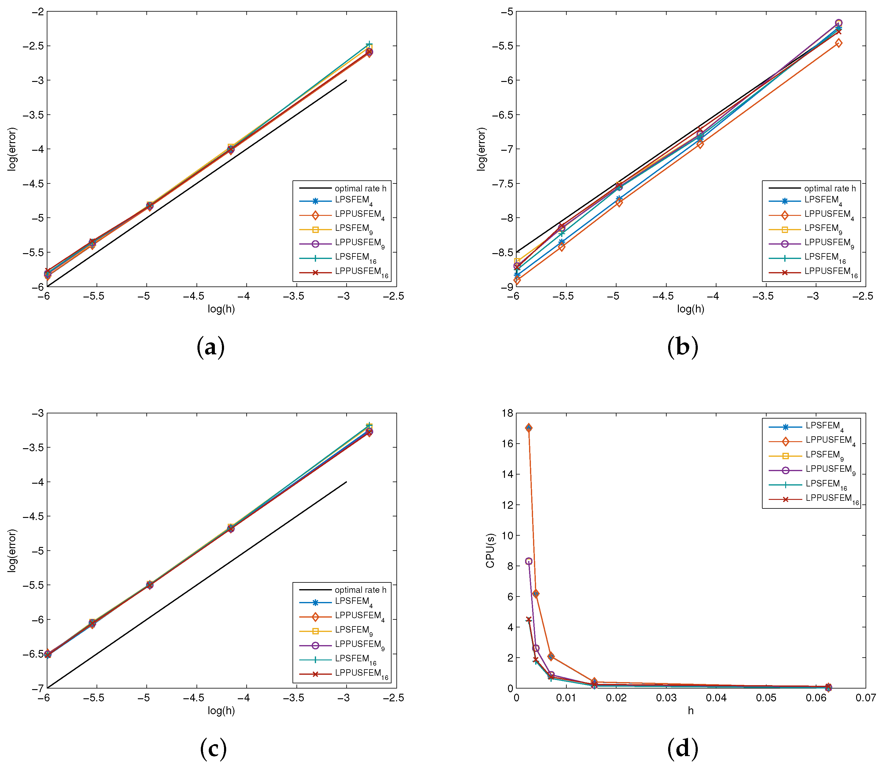
6.1. Test 1
- (a)
- Convergence orders (for the velocity, pressure, and piezometric head) of the four algorithm are all one with respect to the fine mesh size h, which agrees with the theoretical results;
- (b)
- LPSFEM derives a better approximation than LPFEM since the errors of LPSFEM are less than that of LPFEM. The same conclusion is suitable for the comparison of LPPUSFEM and LPPUFEM;
- (c)
- LPSFEM and LPPUSFEM exhibit almost the same errors, which indicates that the partition of unity functions scarcely ever affect the error accuracy. The same situation happens to LPFEM and LPPUFEM.
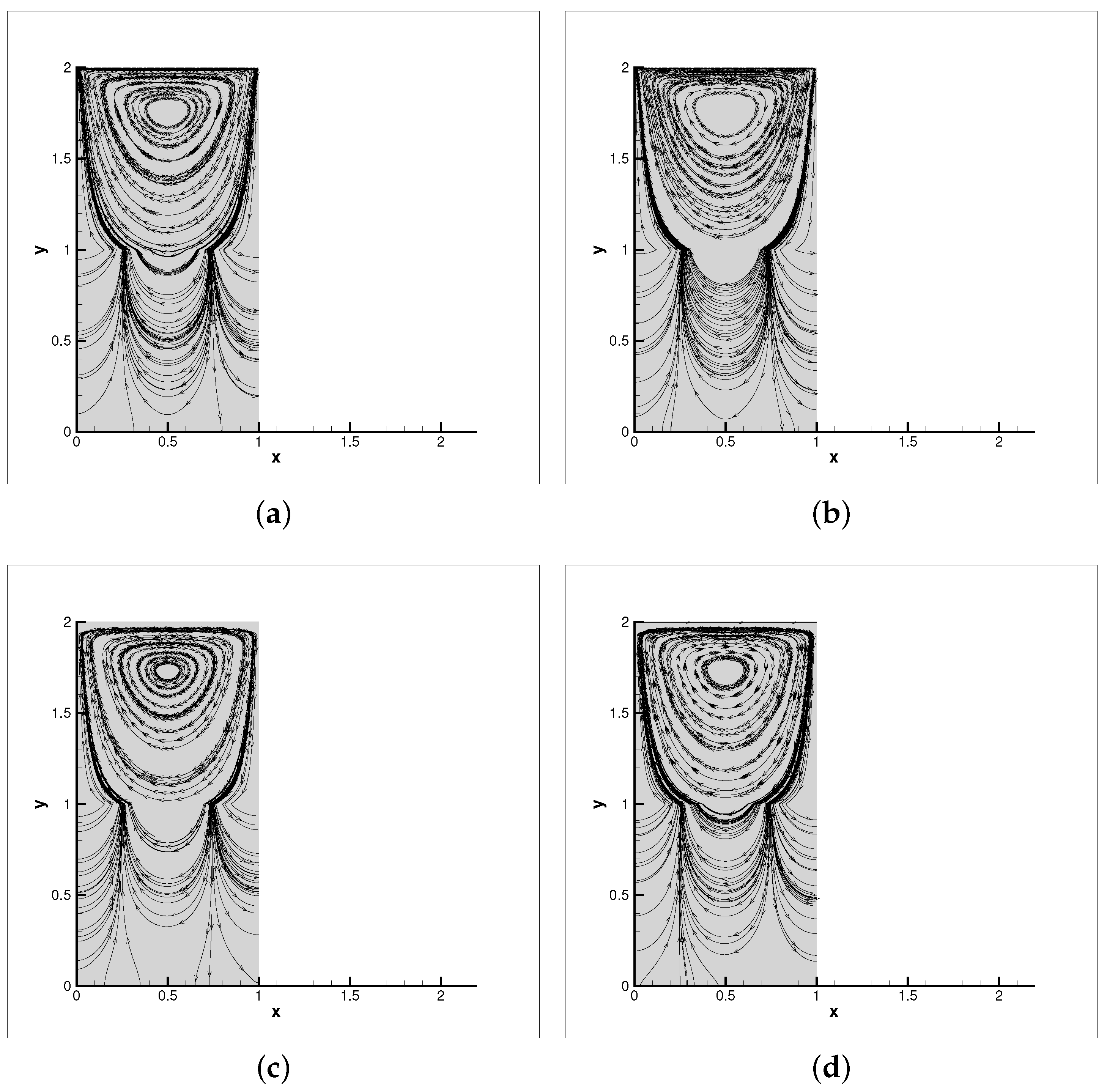
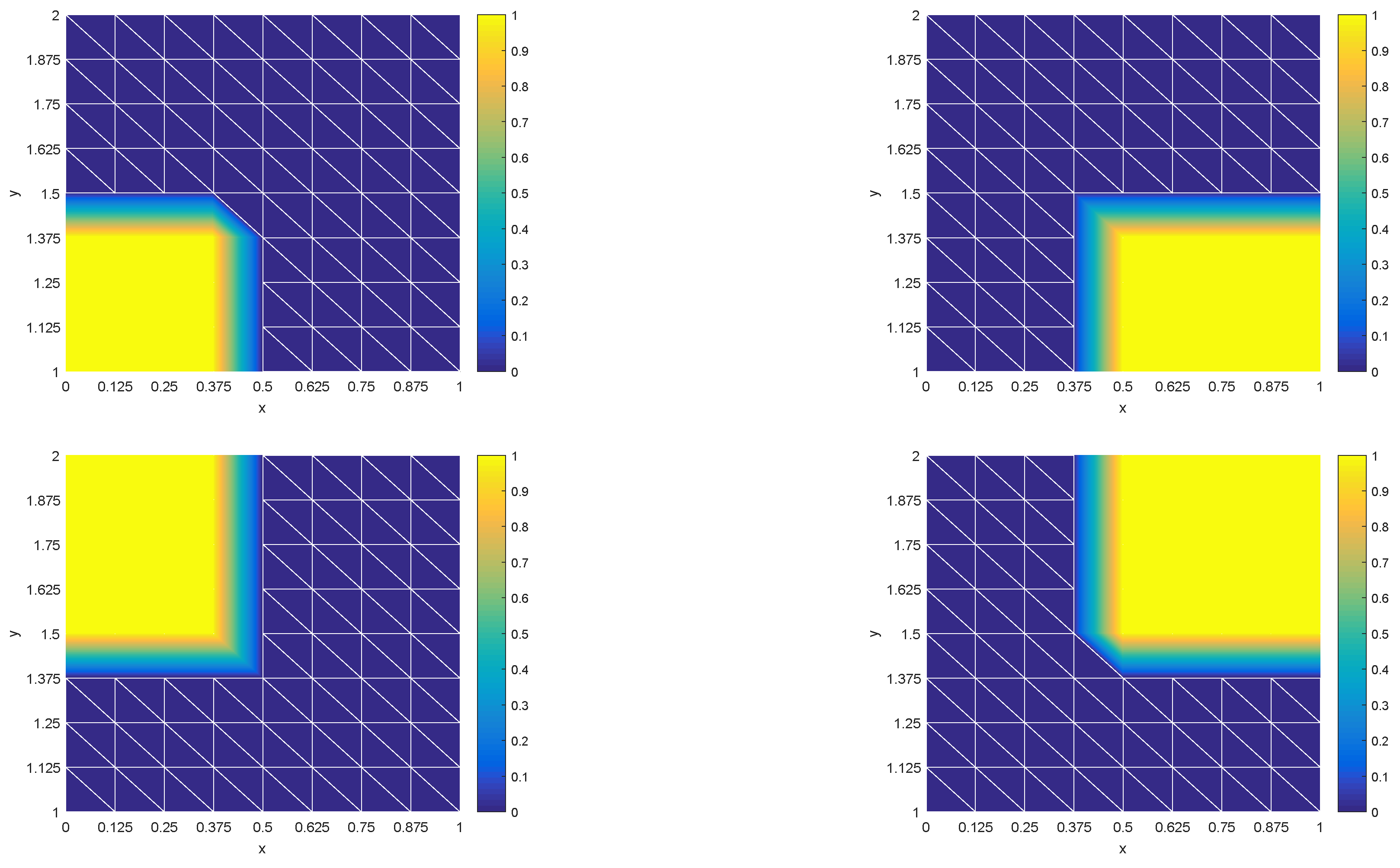
6.2. Test 2
7. Conclusions
Author Contributions
Funding
Data Availability Statement
Conflicts of Interest
References
- Cao, Y.; Gunzburger, M.; Hu, X.; Hua, F.; Wang, X.; Zhao, W. Finite element approximation for Stokes-Darcy flow with Beavers-Joseph interface conditions. SIAM J. Numer. Anal. 2010, 47, 4239–4256. [Google Scholar] [CrossRef]
- Rivire, B.; Yotov, I. Locally conservative coupling of Stokes and Darcy flows. SIAM J. Numer. Anal. 2005, 42, 1959–1977. [Google Scholar] [CrossRef]
- Rui, H.; Zhang, R. A unified stabilized mixed finite element method for coupling Stokes and Darcy flows. Comput. Methods Appl. Mech. Eng. 2009, 198, 2692–2699. [Google Scholar] [CrossRef]
- Cai, M.; Mu, M.; Xu, J. Numerical solution to a mixed Navier-Stokes/Darcy model by the two-grid approach. SIAM J. Numer. Anal. 2009, 47, 3325–3338. [Google Scholar] [CrossRef]
- Du, G.; Zuo, L. A two-grid method with backtracking for the mixed Stokes/Darcy model. J. Numer. Math. 2021, 29, 39–46. [Google Scholar]
- Mu, M.; Xu, J. A two-grid method of a mixed Stokes-Darcy model for coupling fluid flow with porous media flow. SIAM J. Numer. Anal. 2007, 45, 1801–1813. [Google Scholar] [CrossRef]
- Cai, M.; Mu, M. A multilevel decoupled method for a mixed Stokes/Darcy model. J. Comput. Appl. Math. 2012, 236, 2452–2465. [Google Scholar] [CrossRef]
- Chen, W.; Gunzburger, M.; Hua, F.; Wang, X. A parallel Robin-Robin domain decomposition method for the Stokes-Darcy system. SIAM J. Numer. Anal. 2011, 49, 1064–1084. [Google Scholar] [CrossRef]
- He, X.; Li, J.; Lin, Y.; Ming, J. A domain decomposition method for the steady-state Navier-Stokes-Darcy model with the Beavers-Joseph interface condition. SIAM J. Sci. Comput. 2015, 37, S264–S290. [Google Scholar] [CrossRef]
- Jiang, B. A parallel domain decomposition method for coupling of surface and groundwarter flows. Comput. Methods Appl. Mech. Eng. 2009, 198, 947–957. [Google Scholar] [CrossRef]
- Sun, Y.; Sun, W.; Zheng, H. Domain decomposition method for the fully-mixed Stokes-Darcy coupled problem. Comput. Methods Appl. Mech. 2021, 374, 113578. [Google Scholar] [CrossRef]
- Xu, J.; Zhou, A. Local and parallel finite element algorithms based on two-grid discretizations. Math. Comput. 2000, 69, 881–909. [Google Scholar] [CrossRef]
- Xu, J.; Zhou, A. Local and parallel finite element algorithms based on two-grid discretizations for nonlinear problems. Adv. Comput. Math. 2001, 14, 293–327. [Google Scholar] [CrossRef]
- He, Y.; Xu, J.; Zhou, A.; Li, J. Local and parallel finite element algorithms for the Stokes problem. Numer. Math. 2008, 109, 415–434. [Google Scholar] [CrossRef]
- He, Y.; Xu, J.; Zhou, A. Local and parallel finite element algorithms for the Navier-Stokes problem. J. Comput. Math. 2006, 24, 227–238. [Google Scholar]
- Shang, Y.; He, Y. Parallel iterative finite element algorithms based on full domain partition for the stationary Navier-Stokes equations. Appl. Numer. Math. 2010, 60, 719–737. [Google Scholar] [CrossRef]
- Zheng, B.; Shang, Y. Local and parallel stabilized finite element algorithms based on the lowest equal-order elements for the steady Navier-Stokes equations. Math. Comput. Simul. 2020, 178, 464–484. [Google Scholar] [CrossRef]
- Du, G.; Zuo, L. Local and parallel finite element methods for the coupled Stokes/Darcy model. Numer. Algor. 2021, 87, 1593–1611. [Google Scholar] [CrossRef]
- Zuo, L.; Du, G. A parallel two-grid linearized method for the coupled Navier-Stokes-Darcy problem. Numer. Algor. 2018, 77, 151–165. [Google Scholar] [CrossRef]
- Zhang, Y.; Hou, Y.; Shan, L.; Dong, X. Local and parallel finite element algorithm for stationary incompressible magnetohydrodynamics. Numer. Methods Partial Differ. Equ. 2017, 33, 1513–1539. [Google Scholar] [CrossRef]
- Du, G.; Zuo, L. A Parallel Partition of Unity Scheme Based on Two-Grid Discretizations for the Navier-Stokes Problem. J. Sci. Comput. 2018, 75, 1445–1462. [Google Scholar] [CrossRef]
- Yu, J.; Shi, F.; Zheng, H. Local and parallel finite element algorithms based on the partition of unity for the stokes problem. SIAM J. Sci. Comput. 2014, 36, C547–C567. [Google Scholar] [CrossRef]
- Song, L.; Gao, M. A posteriori error estimates for the stabilization of low-order mixed finite elements for the Stokes problem. Comput. Methods Appl. Mech. Eng. 2014, 279, 410–424. [Google Scholar] [CrossRef]
- Dohrmann, C.; Bochev, P. A stabilized finite element method for the Stokes problem based on polynomial pressure projections. Int. J. Numer. Meth. Fluids 2004, 46, 183–201. [Google Scholar] [CrossRef]
- He, Y.; Li, J. A stabilized finite element method based on local polynomial pressure projection for the stationary Navier-Stokes equations. Appl. Numer. Math. 2008, 58, 1503–1514. [Google Scholar] [CrossRef]
- Shang, Y. A parallel stabilized finite element method based on the lowest equal-order elements for incompressible flows. Computing 2020, 102, 65–81. [Google Scholar] [CrossRef]
- Li, J.; He, Y.; Chen, Z. A new stabilized finite element method for the transient Navier-Stokes equations. Comput. Methods Appl. Mech. Eng. 2007, 197, 22–35. [Google Scholar] [CrossRef]
- Li, J.; He, Y. A stabilized finite element method based on two local Gauss integrations for the Stokes equations. J. Comp. Appl. Math. 2008, 214, 58–65. [Google Scholar] [CrossRef]
- Li, R.; Li, J.; Chen, Z.; Gao, Y. A stabilized finite element method based on two local Gauss integrations for a coupled Stokes-Darcy problem. J. Comput. Appl. Math. 2016, 292, 92–104. [Google Scholar] [CrossRef]
- Zheng, H.; Hou, Y.; Shi, F.; Song, L. A finite element variational multiscale method for incompressible flows based on two local Gauss integrations. J. Comput. Phys. 2009, 228, 5961–5977. [Google Scholar] [CrossRef]
- Melenk, J.M.; Babusˇka, I. The Partition of Unity Finite Element Method: Basic Theory and Applications. Comput. Meth. Appl. Mech. Eng. 1996, 139, 289–314. [Google Scholar] [CrossRef]
- Lions, J.L.; Magenes, E. Non-Homogeneous Boundary Value Problems and Applications; Springer: New York, NY, USA; Heidelberg, Germany, 1972; Volume 1. [Google Scholar]
- Hou, Y. Optimal error estimates of a decoupled scheme based on two-grid finite element for mixed Stokes-Darcy model. Appl. Math. Lett. 2016, 57, 90–96. [Google Scholar] [CrossRef]


| 4 | 16 | − | − | ||
| 8 | 64 | ||||
| 12 | 144 |
| 4 | 16 | − | − | ||
| 8 | 64 | ||||
| 12 | 144 |
| 4 | 16 | − | − | ||
| 8 | 64 | ||||
| 12 | 144 |
| 4 | 16 | − | − | ||
| 8 | 64 | ||||
| 12 | 144 |
| 4 | 16 | − | − | ||
| 8 | 64 | ||||
| 12 | 144 |
| 4 | 16 | − | − | ||
| 8 | 64 | ||||
| 12 | 144 |
| 16 | ||||
| 64 | ||||
| 144 | ||||
| 256 | ||||
| 400 |
Disclaimer/Publisher’s Note: The statements, opinions and data contained in all publications are solely those of the individual author(s) and contributor(s) and not of MDPI and/or the editor(s). MDPI and/or the editor(s) disclaim responsibility for any injury to people or property resulting from any ideas, methods, instructions or products referred to in the content. |
© 2023 by the authors. Licensee MDPI, Basel, Switzerland. This article is an open access article distributed under the terms and conditions of the Creative Commons Attribution (CC BY) license (https://creativecommons.org/licenses/by/4.0/).
Share and Cite
Han, J.; Du, G. Local and Parallel Stabilized Finite Element Methods Based on the Lowest Equal-Order Elements for the Stokes–Darcy Model. Mathematics 2023, 11, 4820. https://doi.org/10.3390/math11234820
Han J, Du G. Local and Parallel Stabilized Finite Element Methods Based on the Lowest Equal-Order Elements for the Stokes–Darcy Model. Mathematics. 2023; 11(23):4820. https://doi.org/10.3390/math11234820
Chicago/Turabian StyleHan, Jing, and Guangzhi Du. 2023. "Local and Parallel Stabilized Finite Element Methods Based on the Lowest Equal-Order Elements for the Stokes–Darcy Model" Mathematics 11, no. 23: 4820. https://doi.org/10.3390/math11234820
APA StyleHan, J., & Du, G. (2023). Local and Parallel Stabilized Finite Element Methods Based on the Lowest Equal-Order Elements for the Stokes–Darcy Model. Mathematics, 11(23), 4820. https://doi.org/10.3390/math11234820