
Unveiling Deep Learning Insights: A Specialized Analysis of Sucker Rod Pump Dynamographs, Emphasizing Visualizations and Human Insight


Abstract
:1. Introduction
- We developed and evaluated 11 customized deep learning models for classifying 11 unique dynamograph classes.
- We introduced a novel framework, utilizing Grad–CAM, that unveils the internal decision-making processes of these models, mitigating the ”black box” issue.
- We conducted an unprecedented comparative study measuring the models against human experts, offering insights into their relative strengths and weaknesses.
- We facilitated a more comprehensive understanding of dynamograph analysis, by blending machine precision and human interpretive insights.
2. Background
2.1. Traditional Interpretation of Dyna Cards
2.1.1. Fluid Load and Working Fluid Level
- —working or net fluid level from the surface (ft)
- —fluid load (lb)
- —specific gravity of the fluid produced
- —plunger area (inch2)
2.1.2. Wellbore Pressures
- —pump intake pressure (psi)
- D—pump setting depth (ft)
- —gas pressure above the working fluid level
- (psi)
- —surface casing pressure (psi)
- —flowing BHP inside the wellbore (psi)
- —depth of the perforations (ft)
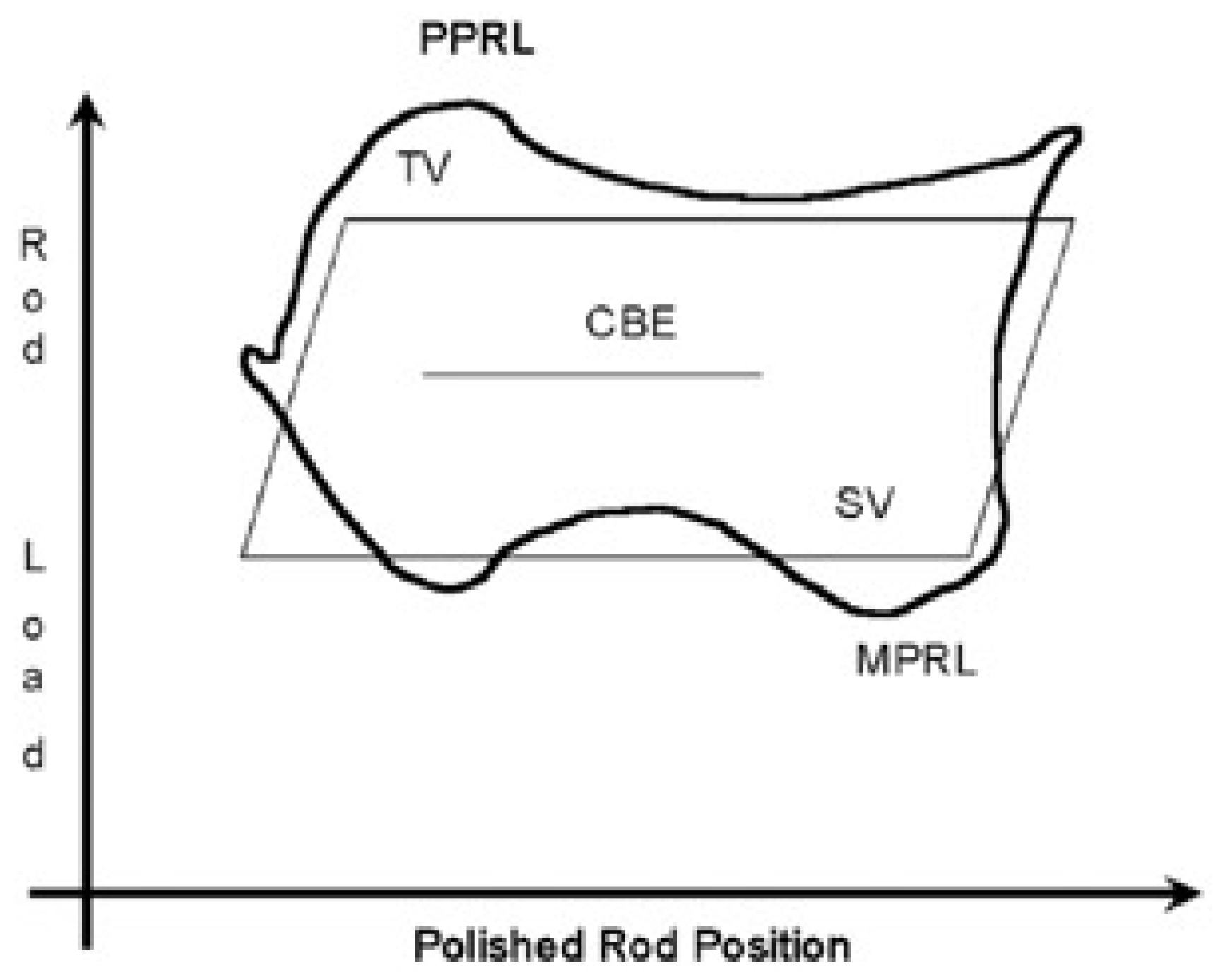
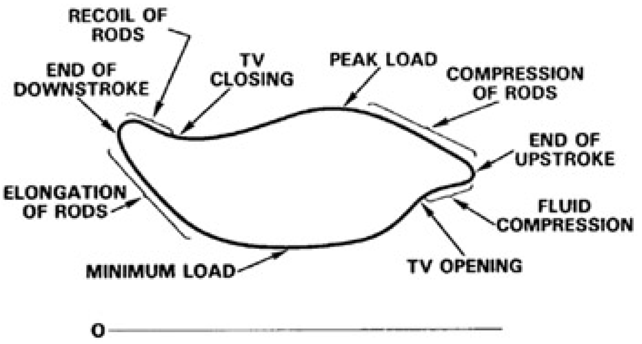
2.1.3. Normal Operations Dynamograph
- The pump’s barrel and plunger are in impeccable condition.
- The standing and traveling valves exhibit no leaks.
- All friction forces along the rod string result from viscous damping.
- Only single-phase liquid enters the pump barrel.
- The barrel completely fills up during the upstroke.
2.1.4. Detailed Analysis and Pattern Recognition
Gas Interference
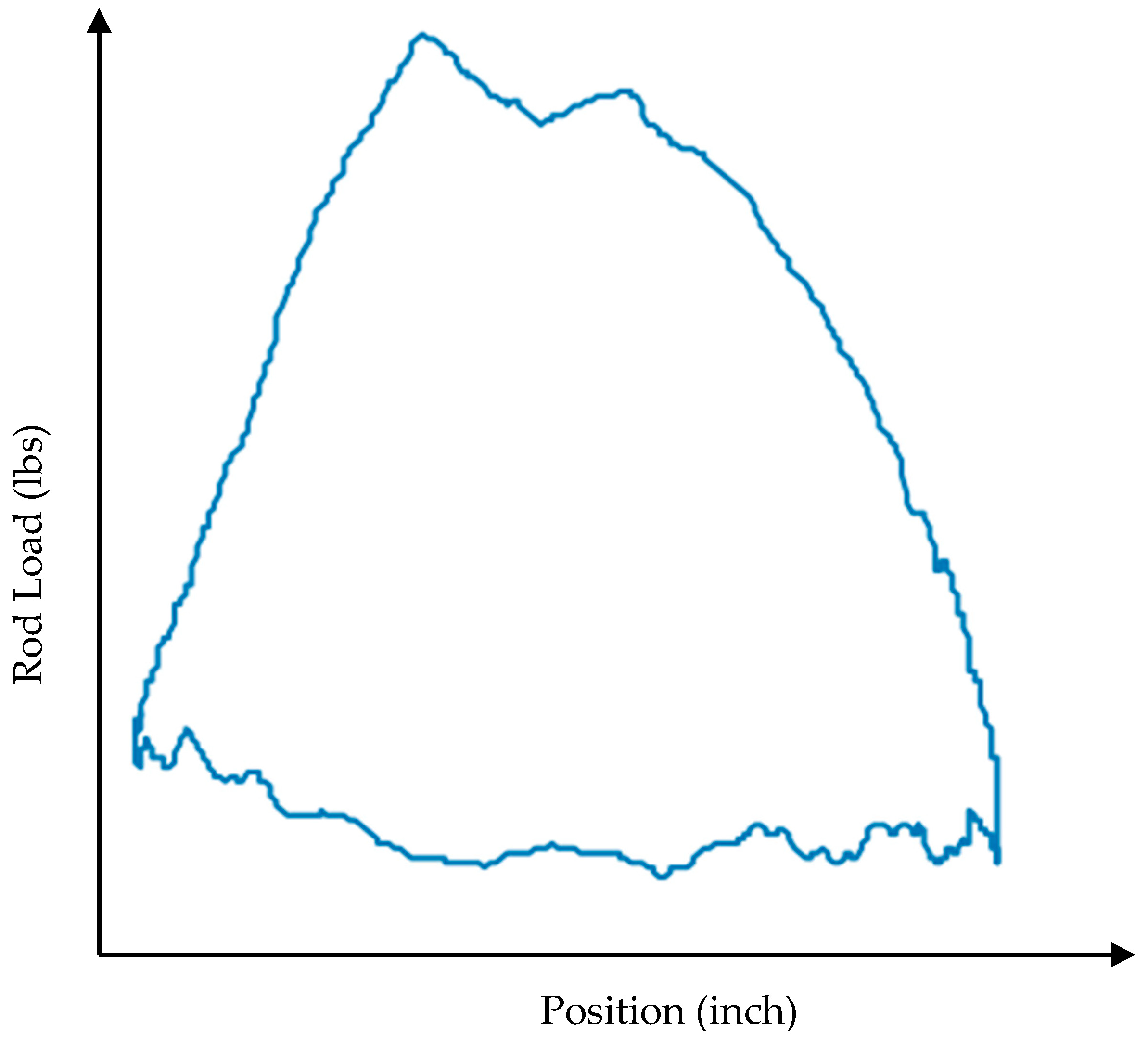
Highly Viscous Fluid
Gas Locking
Fluid Pound
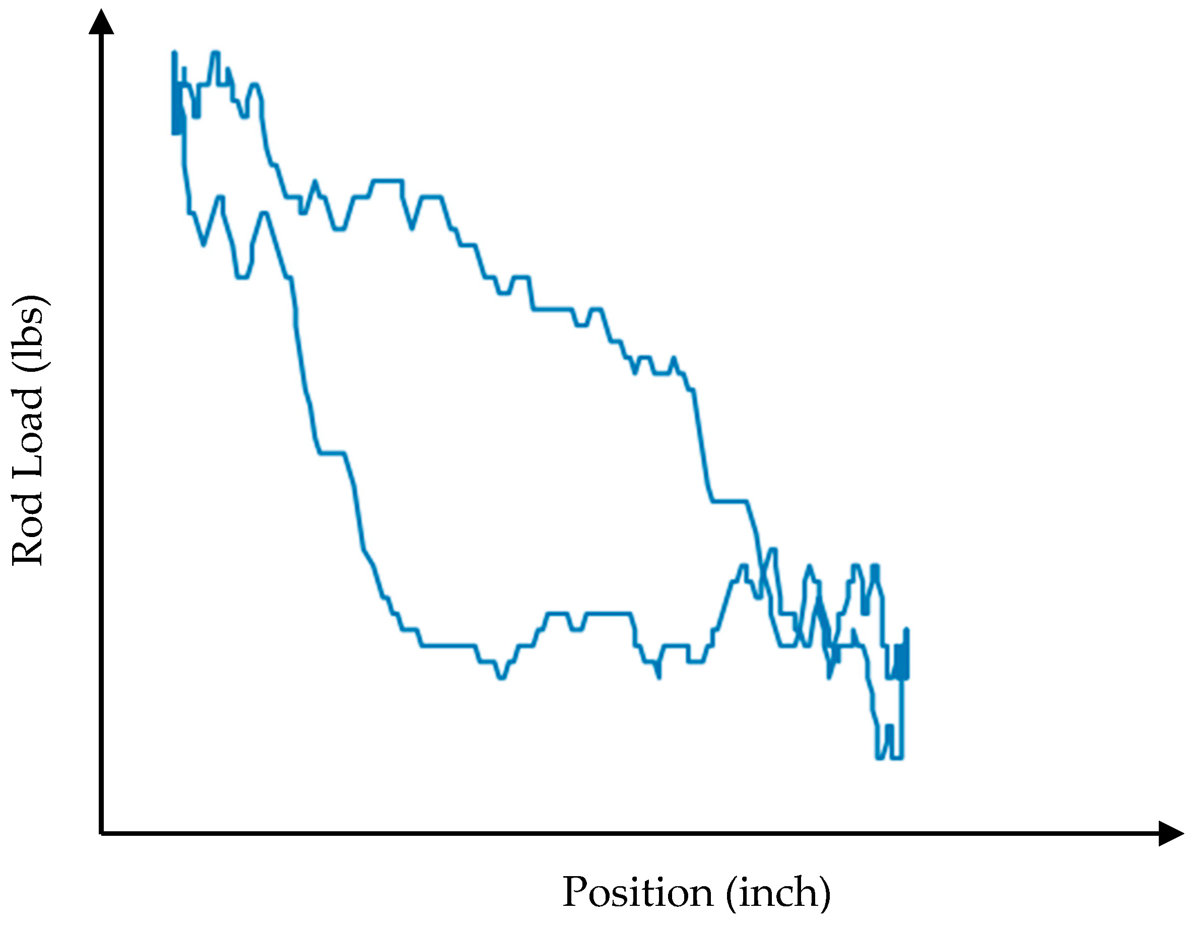
TV Leakage
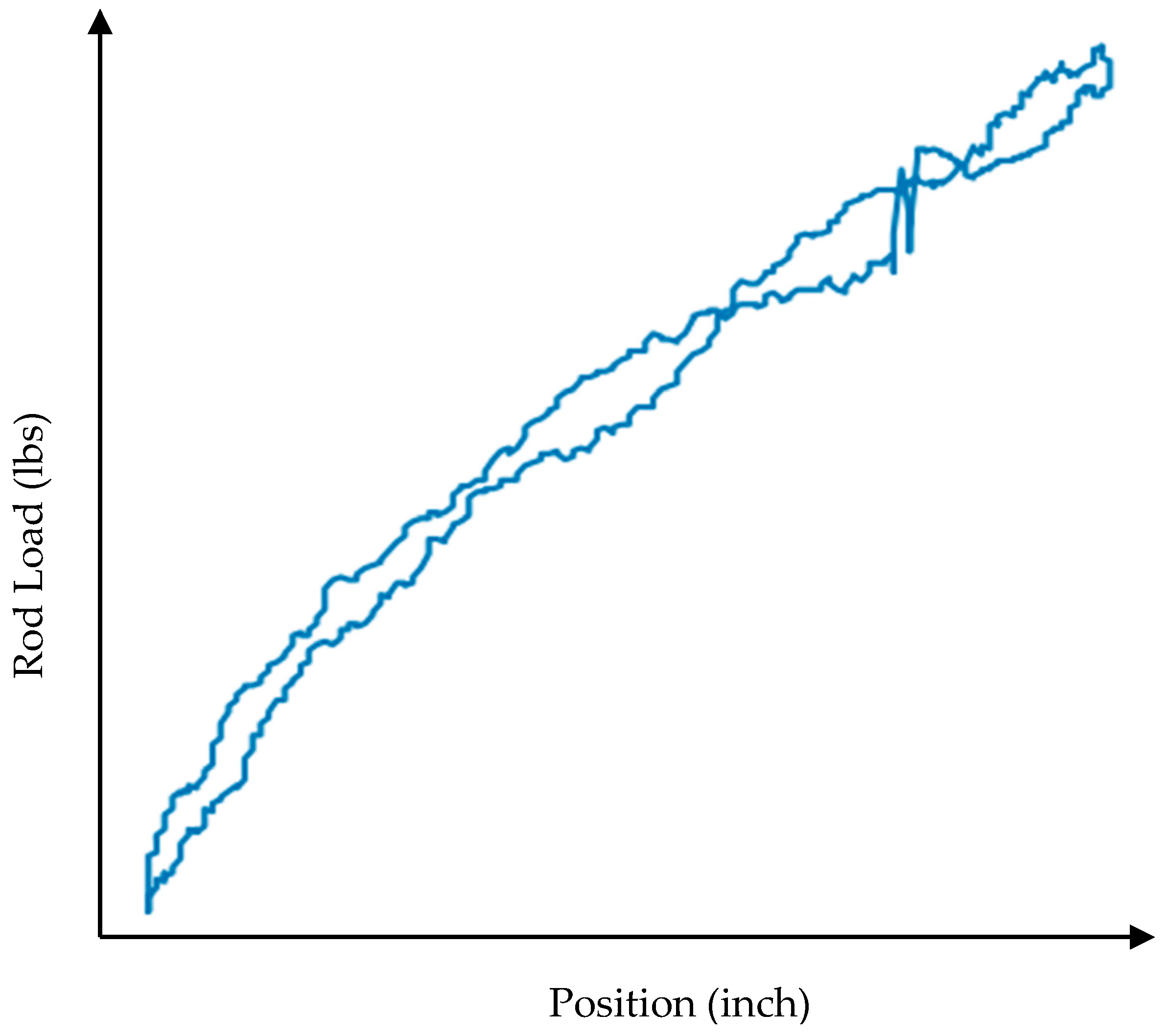
Flow through the Pump
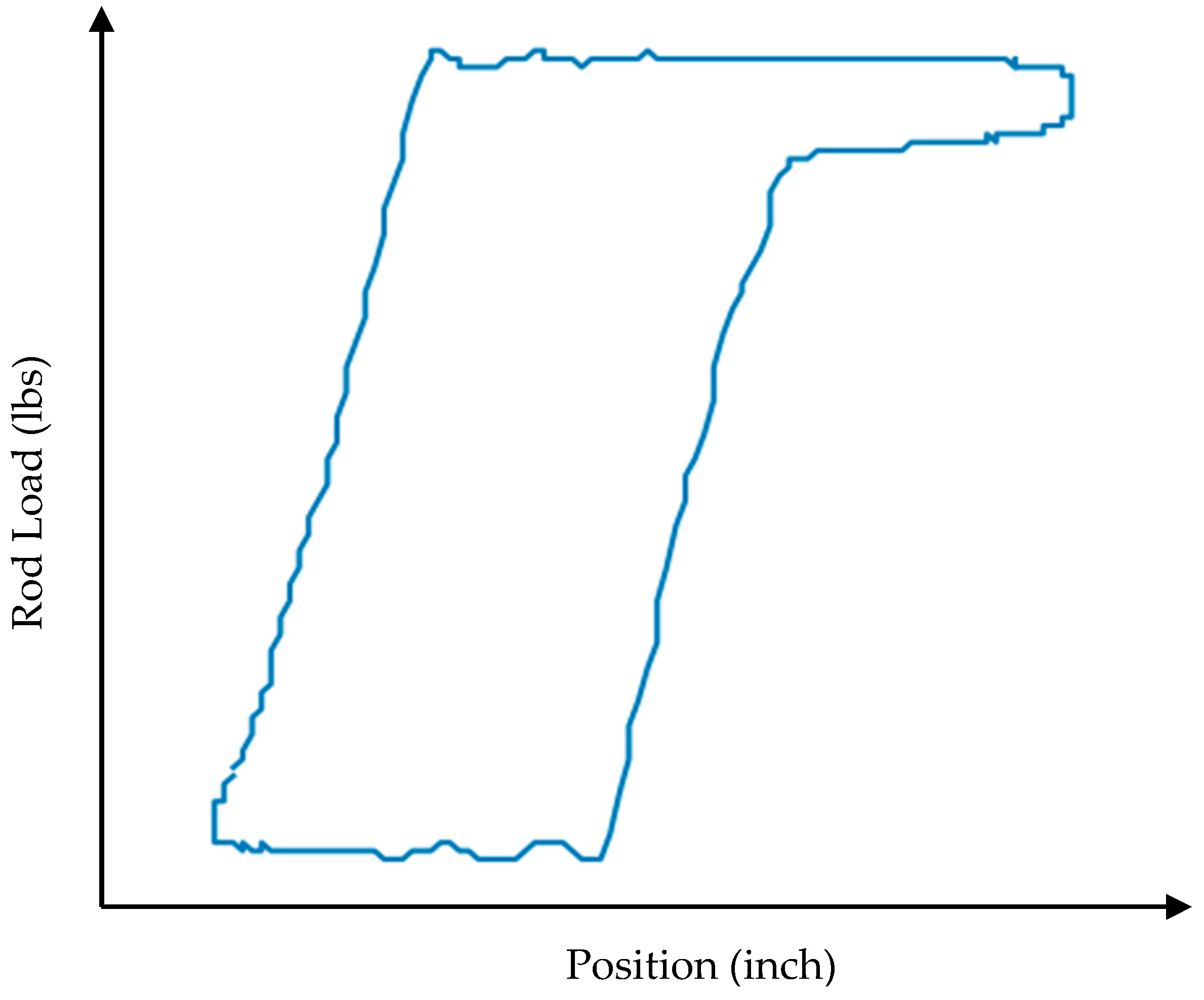
Stuck Plunger
Tagging
3. Related Work
4. Materials and Method
4.1. Dataset Description
4.2. Models Description
- DenseNet121 possesses 121 layers, ensuring comprehensive feature extraction and a complex representational capability.
- DenseNet161 escalates in complexity with 161 layers, enhancing the model’s capacity to discern intricate patterns.
- DenseNet169 offers a balanced performance with its 169 layers, standing as a middle ground in complexity.
- DenseNet201 tops the list with 201 layers, underlining an advanced capacity for the most detailed feature extraction.
- ResNet18 is a fundamental model with 18 layers, ideal for simpler tasks and swift computations.
- ResNet34, with 34 layers, scales up in capacity, offering a more nuanced feature extraction.
- ResNet50 strikes a balance with 50 layers, aligning computational efficiency with enhanced performance.
- ResNet101, having 101 layers, is tailored for intricate tasks, ensuring in-depth pattern recognition.
- ResNet152 is the pinnacle, with 152 layers, engineered for the most intricate feature extraction and pattern recognition.
4.3. Grad-CAM
4.4. Hyperparameter Tuning
4.5. Framework for Dyna Card Type Prediction and Visual Interpretation of Model Decisions
5. Results and Discussion
6. Conclusions
Author Contributions
Funding
Data Availability Statement
Conflicts of Interest
References
- Alemi, M.; Jalalifar, H.; Kamali, G.R.; Kalbasi, M. A mathematical estimation for artificial lift systems selection based on ELECTRE model. J. Pet. Sci. Eng. 2011, 78, 193–200. [Google Scholar] [CrossRef]
- Golan, M.; Whitson, H.C. Well Performance, 2nd ed.; Prentice Hall: Hoboken, NJ, USA, 1995. [Google Scholar]
- Boomer, P.M.; Podio, A.L. The Beam Lift Handbook; PETEX: Austin, TX, USA, 2015. [Google Scholar]
- Zhang, A.; Gao, X. Fault diagnosis of sucker rod pumping systems based on Curvelet Transform and sparse multi-graph regularized extreme learning machine. Int. J. Comput. Intell. Syst. 2018, 11, 428–437. [Google Scholar] [CrossRef]
- Bello, O.; Dolberg, E.; Teodoriu, C.; Karami, H.; Devegowdva, D. Transformation of academic teaching and research: Development of a highly automated experimental sucker rod pumping unit. J. Pet. Sci. Eng. 2020, 190, 107087. [Google Scholar] [CrossRef]
- Gibbs, S.; Neely, A. Computer diagnosis of down-hole conditions in sucker rod pumping wells. J. Pet. Technol. 1966, 18, 91–98. [Google Scholar] [CrossRef]
- Ordonez, B.; Codas, A.; Moreno, U. Improving the Operational Conditions for the Sucker-rod Pumping System. In Proceedings of the 2009 IEEE Control Applications, (CCA) & Intelligent Control, (ISIC), St. Petersburg, Russia, 8–10 July 2009; IEEE: Piscataway, NJ, USA, 2009; pp. 1259–1264. [Google Scholar]
- Li, K.; Gao, X.-W.; Tian, Z.; Qiu, Z. Using the curve moment and the PSO-SVM method to diagnose downhole conditions of a sucker rod pumping unit. Pet. Sci. 2013, 10, 73–80. [Google Scholar] [CrossRef]
- Xu, P.; Xu, S.; Yin, H. Application of self-organizing competitive neural network in fault diagnosis of suck rod pumping system. J. Pet. Sci. Eng. 2007, 58, 43–48. [Google Scholar] [CrossRef]
- Cheng, H.; Yu, H.; Zeng, P.; Osipov, E.; Li, S.; Vyatkin, V. Automatic Recognition of Sucker-Rod Pumping System Working Conditions Using Dynamometer Cards with Transfer Learning and SVM. Sensors 2020, 20, 5659. [Google Scholar] [CrossRef]
- Bezerra, M.A.D.; Schnitman, L.; Baretto Filho, M.d.A.; de Souza, J.A.M.F. Pattern Recognition for Downhold Dynamometer Card in Oil Rod Pump System using Artificial Neural Networks. In Proceedings of the 11th International Conference on Enterprise Information Systems, Volume AIDSS, Milan, Italy, 6–10 May 2009; pp. 351–355. [Google Scholar]
- Zhao, H.; Wang, J.; Gao, P. A Deep Learning Approach for Condition-based Monitoring and Fault Diagnosis of Rod Pump. Serv. Trans. Internet Things (STIOT) 2017, 1, 32–42. [Google Scholar] [CrossRef]
- Ali, S.; Abuhmed, T.; El-Sappagh, S.; Muhammad, K.; Alonso-Moral, J.M.; Confalonieri, R.; Guidotti, R.; Del Ser, J.; Díaz-Rodríguez, N.; Herrera, F. Explainable artificial intelligence (XAI): What we know and what is left to attain trustworthy artificial intelligence. Inf. Fusion 2023, 99, 101805. [Google Scholar] [CrossRef]
- Brożek, B.; Furman, M.; Jakubiec, M.; Kucharzyk, B. The black box problem was revisited. Real and imaginary challenges for automated legal decision-making. Artif. Intell. Law 2023. [Google Scholar] [CrossRef]
- Voulodimos, A.; Doulamis, N.; Doulamis, A.; Protopapadakis, E. Deep learning for computer vision: A brief review. Comput. Intell. Neurosci. 2018, 2018, 7068349. [Google Scholar] [CrossRef] [PubMed]
- O’Mahony, N.; Campbell, S.; Carvalho, A.; Harapanahalli, S.; Hernandez, G.V.; Krpalkova, L.; Walsh, J. Deep learning vs. traditional computer vision. In Advances in Computer Vision, Proceedings of the 2019 Computer Vision Conference (CVC), Las Vegas, NV, USA, 2–3 May 2019; Springer: Cham, Switzerland, 2020; Volume 1, pp. 128–144. [Google Scholar]
- Selvaraju, R.R.; Cogswell, M.; Das, A.; Vedantam, R.; Parikh, D.; Batra, D. Grad-cam: Visual explanations from deep networks via gradient-based localization. In Proceedings of the IEEE International Conference on Computer Vision, Venice, Italy, 22–29 October 2017; IEEE: Piscataway, NJ, USA, 2017; pp. 618–626. [Google Scholar]
- Kemler, E. An Investigation of Experimental Methods of Determining Sucker-Rod Loads. Trans. AIME 1936, 118, 89–99. [Google Scholar] [CrossRef]
- Gipson, F.W.; Swaim, H.W. The beam pumping design chain. In Proceedings of the 31st Annual Southwestern Petroleum Short Course, Lubbock, TX, USA, 23–25 April 1984; Texas Tech University: Lubbock, TX, USA, 1984; pp. 296–376. [Google Scholar]
- American Petroleum Institute. API RP 11L Recommended Practice for Design Calculations for Sucker Rod Pumping Systems (Conventional Units), 4th ed.; American Petroleum Institute: Washington, DC, USA, 1988. [Google Scholar]
- Soza, R.L. Review of Downhole Dynamometer Testing. In Proceedings of the Permian Basin Oil and Gas Recovery Conference, Midland, TX, USA, 27–29 March 1998. [Google Scholar]
- Economides, M.J.; Hill, D.A.; Ehlig Economides, C. Petroleum Production Systems; Prentice Hall: Hoboken, NJ, USA, 1994. [Google Scholar]
- Russell, J.H., Jr. Interpretation of Dynamometer Cards. World Oil, July 1953. [Google Scholar]
- Fagg, L.W. Dynamometer charts and well weighing. Pet Trans AIME 1950, 189, 165–174. [Google Scholar] [CrossRef]
- Milovzorov, G.; Ilyin, A.; Shirobokov, P. Diagnostics of the condition of sucker-rod pumping units after the analysis of dynamogram cards. MATEC Web Conf. 2019, 298, 00137. [Google Scholar] [CrossRef]
- API. API Bul 11L2 Catalog of Analog Computer Dynamometer Cards, 1st ed.; American Petroleum Institute: Dallas, TX, USA, 1969. [Google Scholar]
- Podio, A.L.; McCoy, J.N.; Rowlan, O.L.; Becker, D. Dynamometer analysis plots improve ability to troubleshoot and analyze problems. In Proceedings of the 50th Annual Southwestern Petroleum Short Course, Lubbock, TX, USA, 16–17 April 2003; Texas Tech University: Lubbock, TX, USA, 2003; pp. 160–176. [Google Scholar]
- Takacs, G. Sucker-Rod Pumping Handbook: Production Engineering Fundamentals and Long-Stroke Rod Pumping; Elsevier Science: New York, NY, USA, 2015. [Google Scholar]
- Tripp, H. A review: Analyzing beam-pumped wells. J. Pet. Technol. 1989, 41, 457–458. [Google Scholar] [CrossRef]
- McCoy, J.N.; Rowlan, O.L.; Podio, A.L. Pump card analysis simplified and improved. In Proceedings of the 52nd Annual Southwestern Petroleum Short Course, Lubbock, TX, USA, 20–21 April 2005; Texas Tech University: Lubbock, TX, USA, 2005; pp. 154–164. [Google Scholar]
- Zhang, R.; Yin, Y.; Xiao, L.; Chen, D. Calculation Method for Inflow Performance Relationship in Sucker Rod Pump Wells Based on Real-Time Monitoring Dynamometer Card. Geofluids 2020, 2020, 8884988. [Google Scholar] [CrossRef]
- Derek, H.J.; Jennings, J.W.; Morgan, S.M. EXPROD: Expert Advisor Program for Rod Pumping. In Proceedings of the SPE Annual Technical Conference and Exhibition, Dallas, TX, USA, 27–30 September 1988. [Google Scholar]
- Takács, G. Use of Conventional Dynamometer Cards in the Analysis of Sucker-Rod Pumped Installations. Engineering 2001. [Google Scholar]
- Nascimento, J.; Maitelli, A.; Maitelli, C.; Cavalcanti, A. Diagnostic of Operation Conditions and Sensor Faults using Machine Learning in Sucker-Rod Pumping Wells. Sensors 2021, 21, 4546. [Google Scholar] [CrossRef]
- Sharaf, S.A.; Bangert, P.; Fardan, M.; Alqassab, K.; Abubakr, M.; Ahmed, M. Beam-Pump Dynamometer Card Classification Using Machine Learning. In Proceedings of the SPE Middle East Oil and Gas Show and Conference, Manama, Bahrain, 18–21 March 2019. [Google Scholar]
- Janiesch, C.; Zschech, P.; Heinrich, K. Machine learning and deep learning. Electron. Mark. 2021, 31, 685–695. [Google Scholar] [CrossRef]
- Xu, Y.; Qian, W.; Li, N.; Li, H. Typical advances of artificial intelligence in civil engineering. Adv. Struct. Eng. 2022, 25, 3405–3424. [Google Scholar] [CrossRef]
- Dreyfus, G. Neural Networks Methodology and Applications, 2nd ed.; Springer: Berlin/Heidelberg, Germany, 2004. [Google Scholar]
- Koroteev, D.; Tekic, Z. Artificial intelligence in oil and gas upstream: Trends, challenges, and scenarios for the future. Energy AI 2021, 3, 100041. [Google Scholar] [CrossRef]
- Sircar, A.; Yadav, K.; Rayavarapu, K.; Bist, N.; Oza, H. Application of machine learning and artificial intelligence in oil and gas industry. Pet. Res. 2021, 6, 379–391. [Google Scholar] [CrossRef]
- Li, H.; Yu, H.; Cao, N.; Tian, H.; Cheng, S. Applications of artificial intelligence in oil and gas development. Arch. Comput. Methods Eng. 2021, 28, 937–949. [Google Scholar] [CrossRef]
- Souza, A.M.F.D.; Bezerra, M.A.D.; Filho, M.D.A.B.; Schnitman, L. Using artificial neural networks for pattern recognition of downhole dynamometer card in oil rod pump system. In Proceedings of the AIKED’09: Artificial Intelligence, Knowledge Engineering and Data Bases, Cambridge, UK, 21–23 February 2009. [Google Scholar]
- He, Y.; Liu, Y.; Shao, S.; Zhao, X.; Liu, G.; Kong, X.; Liu, L. Application of CNN-LSTM in Gradual Changing Fault Diagnosis of Rod Pumping System. Math. Probl. Eng. 2019, 2019, 1–9. [Google Scholar] [CrossRef]
- Serradilla, O.; Zugasti, E.; Ramirez de Okariz, J.; Rodriguez, J.; Zurutuza, U. Adaptable and Explainable Predictive Maintenance: Semi-Supervised Deep Learning for Anomaly Detection and Diagnosis in Press Machine Data. Appl. Sci. 2021, 11, 7376. [Google Scholar] [CrossRef]
- Wang, K.; Wang, Y. How AI Affects the Future Predictive Maintenance: A Primer of Deep Learning. In Advanced Manufacturing and Automation VII; Springer: Singapore, 2018; pp. 1–9. [Google Scholar]
- Jimenez-Cortadi, A.; Irigoien, I.; Boto, F.; Sierra, B.; Rodriguez, G. Predictive Maintenance on the Machining Process and Machine Tool. Appl. Sci. 2020, 10, 224. [Google Scholar] [CrossRef]
- Xu, C.; Fu, L.; Lin, T.; Li, W.; Ma, S. Machine learning in petrophysics: Advantages and limitations. Artifical Intell. Geosci. 2022, 3, 157–161. [Google Scholar] [CrossRef]
- Hong, S.R.; Hullman, J.; Bertini, E. Human Factors in Model Interpretability: Industry Practices, Challenges, and Needs. Proc. ACM Hum.-Comput. Interact. 2020, 4, 1–26. [Google Scholar] [CrossRef]
- Teixeira, A.F.; Secchi, A.R. Machine learning models to support reservoir production optimization. IFAC-Pap. 2019, 52, 498–501. [Google Scholar] [CrossRef]
- Martyushev, D.A.; Ponomareva, I.N.; Zakharov, L.A.; Shadrov, T.A. Application of machine learning for forecasting formation pressure in oil field development. Izv. Tomsk. Politekh. Univ. Inz. Georesursov. 2021, 332, 140–149. [Google Scholar]


| Label | Total | Train | Validation | Test |
|---|---|---|---|---|
| Good dynamograph | 67 | 47 | 10 | 10 |
| Stuck plunger | 227 | 159 | 34 | 34 |
| TV leaking | 133 | 93 | 20 | 20 |
| Gas lock | 40 | 28 | 6 | 6 |
| Pump wear | 1680 | 1176 | 252 | 252 |
| High viscosity | 320 | 224 | 48 | 48 |
| Bottom tagging | 213 | 149 | 32 | 32 |
| Fluid pound | 80 | 56 | 12 | 12 |
| Gas interference | 600 | 420 | 90 | 90 |
| Flowing through pump | 1573 | 1101 | 236 | 236 |
| Polish rod tagging | 160 | 112 | 24 | 24 |
| Model Name | Accuracy | Precision Micro | Precision Macro | Recall Micro | Recall Macro | f1 Micro | f1 Macro |
|---|---|---|---|---|---|---|---|
| DenseNet121_h_1 | 0.836 | 0.836 | 0.334 | 0.836 | 0.411 | 0.836 | 0.368 |
| DenseNet121_h_2 | 0.885 | 0.885 | 0.471 | 0.885 | 0.524 | 0.885 | 0.495 |
| DenseNet121_h_3 | 0.825 | 0.825 | 0.332 | 0.825 | 0.386 | 0.825 | 0.355 |
| DenseNet161_h_1 | 0.932 | 0.932 | 0.848 | 0.932 | 0.846 | 0.932 | 0.844 |
| DenseNet161_h_2 | 0.909 | 0.909 | 0.661 | 0.909 | 0.708 | 0.909 | 0.681 |
| DenseNet161_h_3 | 0.898 | 0.898 | 0.554 | 0.898 | 0.604 | 0.898 | 0.574 |
| DenseNet169_h_1 | 0.914 | 0.914 | 0.686 | 0.914 | 0.705 | 0.914 | 0.694 |
| DenseNet169_h_2 | 0.916 | 0.916 | 0.639 | 0.916 | 0.701 | 0.916 | 0.664 |
| DenseNet169_h_3 | 0.851 | 0.851 | 0.434 | 0.851 | 0.478 | 0.851 | 0.452 |
| DenseNet201_h_1 | 0.919 | 0.919 | 0.737 | 0.919 | 0.767 | 0.919 | 0.748 |
| DenseNet201_h_2 | 0.919 | 0.919 | 0.761 | 0.919 | 0.767 | 0.919 | 0.763 |
| DenseNet201_h_3 | 0.932 | 0.932 | 0.760 | 0.932 | 0.776 | 0.932 | 0.764 |
| ResNet101_h_1 | 0.909 | 0.909 | 0.647 | 0.909 | 0.670 | 0.909 | 0.653 |
| ResNet101_h_2 | 0.789 | 0.789 | 0.243 | 0.789 | 0.321 | 0.789 | 0.274 |
| ResNet101_h_3 | 0.822 | 0.822 | 0.332 | 0.822 | 0.385 | 0.822 | 0.355 |
| ResNet152_h_1 | 0.864 | 0.864 | 0.603 | 0.864 | 0.633 | 0.864 | 0.615 |
| ResNet152_h_2 | 0.909 | 0.909 | 0.743 | 0.909 | 0.761 | 0.909 | 0.748 |
| ResNet152_h_3 | 0.846 | 0.846 | 0.470 | 0.846 | 0.534 | 0.846 | 0.493 |
| ResNet18_h_1 | 0.927 | 0.927 | 0.883 | 0.927 | 0.885 | 0.927 | 0.882 |
| ResNet18_h_2 | 0.812 | 0.812 | 0.330 | 0.812 | 0.411 | 0.812 | 0.360 |
| ResNet18_h_3 | 0.804 | 0.804 | 0.314 | 0.804 | 0.389 | 0.804 | 0.346 |
| ResNet34_h_1 | 0.914 | 0.914 | 0.747 | 0.914 | 0.770 | 0.914 | 0.757 |
| ResNet34_h_2 | 0.945 | 0.945 | 0.892 | 0.945 | 0.869 | 0.902 | 0.945 |
| ResNet34_h_3 | 0.846 | 0.846 | 0.431 | 0.846 | 0.473 | 0.846 | 0.448 |
| ResNet50_h_1 | 0.901 | 0.901 | 0.743 | 0.901 | 0.737 | 0.901 | 0.737 |
| ResNet50_h_2 | 0.901 | 0.901 | 0.661 | 0.901 | 0.658 | 0.901 | 0.655 |
| ResNet50_h_3 | 0.833 | 0.833 | 0.420 | 0.833 | 0.457 | 0.833 | 0.436 |
| ViT_b_16_h_1 | 0.883 | 0.883 | 0.819 | 0.883 | 0.789 | 0.883 | 0.798 |
| ViT_b_16_h_2 | 0.883 | 0.883 | 0.722 | 0.883 | 0.766 | 0.883 | 0.740 |
| ViT_b_16_h_3 | 0.875 | 0.875 | 0.640 | 0.875 | 0.701 | 0.875 | 0.664 |
| ViT_b_32_h_1 | 0.920 | 0.890 | 0.925 | 0.900 | 0.870 | 0.940 | 0.894 |
| ViT_b_32_h_2 | 0.904 | 0.924 | 0.875 | 0.894 | 0.864 | 0.924 | 0.865 |
| ViT_b_32_h_3 | 0.902 | 0.892 | 0.903 | 0.882 | 0.864 | 0.932 | 0.879 |
| Expertise Level | Time Taken (hours) | Accuracy | Precision | Recall | F1 |
|---|---|---|---|---|---|
| Senior domain expert | 16 | 1 | 1 | 1 | 1 |
| Medior domain expert | 16 | 0.925 | 0.878 | 0.877 | 0.877 |
| Junior domain expert | 40 | 0.748 | 0.678 | 0.677 | 0.677 |
| Label | Dynamograph | Explanation from Domain Expert |
|---|---|---|
| Good dynamograph |  | The model focuses its analysis on the critical region of the dynamograph, specifically the area corresponding to the TV (traveling valve) and SV (standing valve) openings. This targeted approach aligns with the methodology employed by experts in assessing optimal dynamograph behavior, concentrating on the essential elements within the inner parallelogram. By scrutinizing this specific segment, the model captures the crucial dynamics, providing a nuanced evaluation that mirrors the expertise applied in evaluating a well-functioning dynamograph |
| Stuck plunger |  | For the “stuck plunger” label, the model accurately identifies the characteristic shape indicative of a stuck plunger. It focuses on specific image segments where this issue is visibly apparent, aligning with expert analysis. |
| TV leaking | 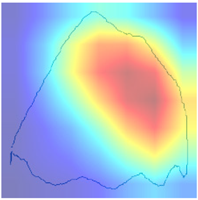 | In the case of “TV leaking”, the model directs its attention to image areas showcasing a decrease in TV load due to fluid column loss, a clear sign of TV leaking issues. |
| Gas lock |  | For the “gas lock” label, the model zeroes in on image sections where there is a noticeable absence of TV and SV opening in each cycle, resulting in non-production of fluid, which is a hallmark of gas lock conditions. |
| Pump wear | 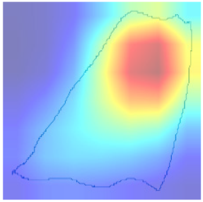 | When analyzing “pump wear”, the model concentrates on image segments where there is a delay in TV load uptake, a phenomenon typically associated with pump wear. |
| High viscosity |  | For “high viscosity”, the model focuses on areas where the fluid’s high viscosity results in a rounded dynamograph shape. This rounded appearance is caused by the delayed opening and closing of valves due to the fluid’s resistance, a common occurrence in high-viscosity conditions. |
| Bottom tagging |  | In the “bottom tagging” scenario, the model’s focus shifts to the lower-left part of the image, where a noticeable drop in load due to mechanical impact on the pump head is evident. This observation is a clear indicator of bottom tagging. |
| Fluid pound | 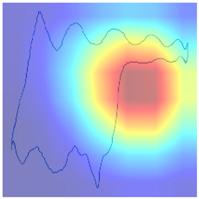 | For the “fluid pound” label, the model concentrates on image sections where the TV opens upon reaching the fluid level within the pump cylinder, a behavior characteristic of fluid pound issues. |
| Gas interference | 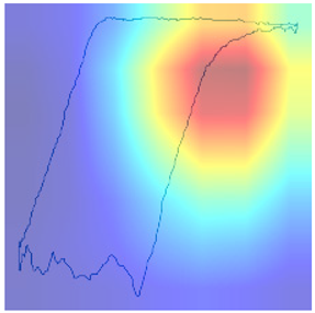 | In the “gas interference” scenario, the model focuses on areas where there is a delay in TV opening due to compression of the gas column within the pump cylinder. This delayed opening is a typical feature observed when gas influences the pump working conditions. |
| Flow through pump | 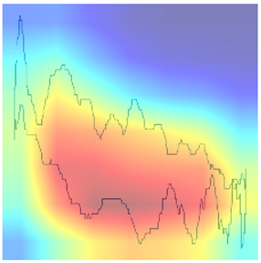 | For the “flow through pump” label, the model analyzes sections where both TV and SV are fully open in each pump cycle, allowing fluid to pass through. This observation indicates a significant reduction in pump efficiency. |
| Polished rod tagging | 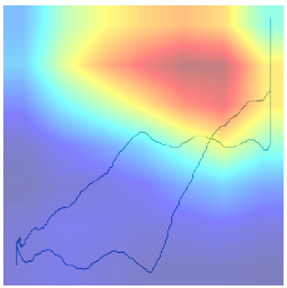 | In the “polished rod tagging” scenario, the model’s focus shifts to the upper-right part of the image, where a noticeable sharp increase in load occurs due to the mechanical impact from the polished rod. This observation is a clear indicator of polished rod tagging. |
| Label/Model Results | Dynamograph with Heat Map | Explanation from Domain Expert |
|---|---|---|
| Bottom tagging/TV leaking | 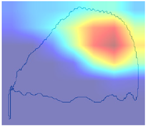 | While the model correctly identifies TV leaking by focusing on the upper segments of the dynamograph, it fails to acknowledge the concurrent presence of tagging. This selective attention to the dynamograph’s upper sections, while accurate to some extent, results in a partial diagnosis, missing the tagging element that is also at play. |
| Stuck plunger/bottom tagging |  | While the model correctly identifies the stuck plunger conditions, it fails to acknowledge the concurrent presence of tagging because it is not focused on the whole dynamograph. This selective attention to the dynamograph’s shape, while accurate to some extent, results in a partial diagnosis, missing the tagging element that is also at play. |
| High viscosity/Pump wear | 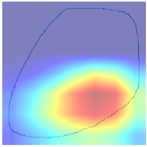 | While the model correctly identifies a high viscosity issue, it is not able to identify pump wear due to not focusing on the upper part of the dynamograph. This selective attention to the dynamograph’s center/low sections, while accurate to some results in a partial diagnosis, misses the pump wear element that is also at play. |
| Polished rod tagging/Gas interference | 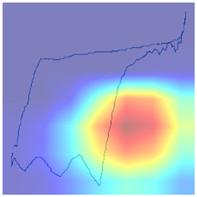 | The model appears to neglect specific dynamograph sections that clearly indicate polished rod tagging. The model is focused on a part of the dynamograph where gas interference is obvious. This oversight suggests a lack of focus or insufficient weighting assigned to the dynamograph areas that are crucial for identifying and confirming the presence of polished rod tagging, warranting further investigation and adjustment. |
Disclaimer/Publisher’s Note: The statements, opinions and data contained in all publications are solely those of the individual author(s) and contributor(s) and not of MDPI and/or the editor(s). MDPI and/or the editor(s) disclaim responsibility for any injury to people or property resulting from any ideas, methods, instructions or products referred to in the content. |
© 2023 by the authors. Licensee MDPI, Basel, Switzerland. This article is an open access article distributed under the terms and conditions of the Creative Commons Attribution (CC BY) license (https://creativecommons.org/licenses/by/4.0/).
Share and Cite
Martinović, B.; Bijanić, M.; Danilović, D.; Petrović, A.; Delibasić, B. Unveiling Deep Learning Insights: A Specialized Analysis of Sucker Rod Pump Dynamographs, Emphasizing Visualizations and Human Insight. Mathematics 2023, 11, 4782. https://doi.org/10.3390/math11234782
Martinović B, Bijanić M, Danilović D, Petrović A, Delibasić B. Unveiling Deep Learning Insights: A Specialized Analysis of Sucker Rod Pump Dynamographs, Emphasizing Visualizations and Human Insight. Mathematics. 2023; 11(23):4782. https://doi.org/10.3390/math11234782
Chicago/Turabian StyleMartinović, Bojan, Milos Bijanić, Dusan Danilović, Andrija Petrović, and Boris Delibasić. 2023. "Unveiling Deep Learning Insights: A Specialized Analysis of Sucker Rod Pump Dynamographs, Emphasizing Visualizations and Human Insight" Mathematics 11, no. 23: 4782. https://doi.org/10.3390/math11234782
APA StyleMartinović, B., Bijanić, M., Danilović, D., Petrović, A., & Delibasić, B. (2023). Unveiling Deep Learning Insights: A Specialized Analysis of Sucker Rod Pump Dynamographs, Emphasizing Visualizations and Human Insight. Mathematics, 11(23), 4782. https://doi.org/10.3390/math11234782