Article

A Deep Learning Neural Network Method Using Linear Eigenvalue Statistics for Schizophrenic EEG Data Classification

1
Department of Automation, Shanghai Jiao Tong University, Shanghai 200240, China
2
Ningbo Artificial Intelligent Institute, Shanghai Jiao Tong University, Ningbo 315000, China
3
Department of Statistic and Actuarial Science, University of Waterloo, Waterloo, ON N2L 3G1, Canada
4
Shanghai Mental Health Center, Shanghai Jiao Tong University School of Medicine, Shanghai Engineering Research Center of Intelligent Psychological Evaluation and Intervention, Shanghai 200001, China
5
School of Electronic Information and Communication, Huazhong University of Science and Technology, Wuhan 430030, China
*
Authors to whom correspondence should be addressed.
Mathematics 2023, 11(23), 4776; https://doi.org/10.3390/math11234776
Submission received: 29 August 2023 / Revised: 12 November 2023 / Accepted: 23 November 2023 / Published: 26 November 2023
(This article belongs to the Special Issue Data-Driven Decision Making: Models, Methods and Applications)

Abstract

:
Electroencephalography (EEG) signals can be used as a neuroimaging indicator to analyze brain-related diseases and mental states, such as schizophrenia, which is a common and serious mental disorder. However, the main limiting factor of using EEG data to support clinical schizophrenia diagnosis lies in the inadequacy of both objective characteristics and effective data analysis techniques. Random matrix theory (RMT) and its linear eigenvalue statistics (LES) can provide an effective mathematical modeling method for exploring the statistical properties of non-stationary nonlinear systems, such as EEG signals. To obtain an accurate classification and diagnosis of schizophrenia, this paper proposes a LES-based deep learning network scheme in which a series of random matrixes, consisting of EEG data sliding window sampling and their eigenvalues, are employed as features for deep learning. Due to the fact that the performance of the LES-based scheme is sensitive to the LES’s test function, the proposed LES-based deep learning network is embedded with two ways of combining LES’s test functions with learning techniques: the first is to have the LES’s test function assigned, while, using the second way, the optimal LES’s test function should be solved in a functional optimization problem. In this paper, various test functions and different optimal learning methods were coupled in experiments. Our results revealed a binary classification accuracy of nearly 90% in distinguishing between healthy controls (HC) and patients experiencing the first episode of schizophrenia (FES). Additionally, we achieved a ternary classification accuracy of approximately 70% by including clinical high risk for psychosis (CHR). The LES-embedded approach yielded notably higher classification accuracy compared to conventional machine learning methods and standard convolutional neural networks. As the performance of schizophrenia classification is strongly influenced by test functions, a functional optimization problem was proposed to identify an optimized test function, and an approximated parameter optimization problem was introduced to limit the search area of suitable basis functions. Furthermore, the parameterization test function optimization problem and the deep learning network were coupled to be synchronously optimized during the training process. The proposal approach achieved higher classification accuracy rates of 96.87% between HC and FES, with an additional 89.06% accuracy when CHR was included. The experimental studies demonstrated that the proposed LES-based method was significantly effective for schizophrenic EEG data classification.

1. Introduction

Schizophrenia is a relatively serious mental illness, and the specific causes of this disease are currently unclear. In clinical practice, it mainly manifests as disharmony in mental activities and various obstacles in terms of emotions, perception, thinking, and other features. If not promptly and effectively treated, it can lead to mental disabilities. Approximately 80% of patients with schizophrenia may experience mental and behavioral abnormalities that do not meet the diagnostic criteria within 2–5 years of onset. In the diagnosis and treatment of schizophrenia, participants are classified as having first-episode schizophrenia (FES), as healthy controls (HC), or as being clinically high risk for psychosis (CHR). CHR is difficult to determine but it is crucial for diagnosis [1]. It is not easy to recognize FES or CHR using EEG data, resulting in obstacles in terms of studying the pathology of schizophrenia.
Electroencephalography (EEG) measures electrical fields produced by an active brain. EEG signal analysis has been used as a diagnostic tool both within and outside of the clinical domain for nearly 90 years. However, EEG still requires strict and objective analysis, as it is a non-stationary nonlinear signal and its interpretation mostly remains intuitive and heuristic. In particular, the cross-channel relations of the signal and its reference to the sources, and hence to certain morphological structures, functional brain structures, or both, are not sufficiently understood and therefore remain a matter of intense research [2]. This study focuses on the application of a resting-state EEG with eyes closed (REC) [3] during the clinical assistant diagnosis and classification of patients with schizophrenia, in an attempt to establish an effective neuroimaging biomarker from EEG signals.
The signal processing of EEG data faces many challenges. It has been previously observed that EEG data feature low signal-to-noise ratios (SNR), non-stationary signals, and high inter-subject variability, which limit the usefulness of EEG applications [4]. A common procedure for EEG-based biometrics involves data collection, preprocessing, feature extraction, and pattern recognition [5]. However, resting-state EEG lacks task-related features, making it difficult to design the best feature for manual extraction. In this study, we considered the non-stationary brain [
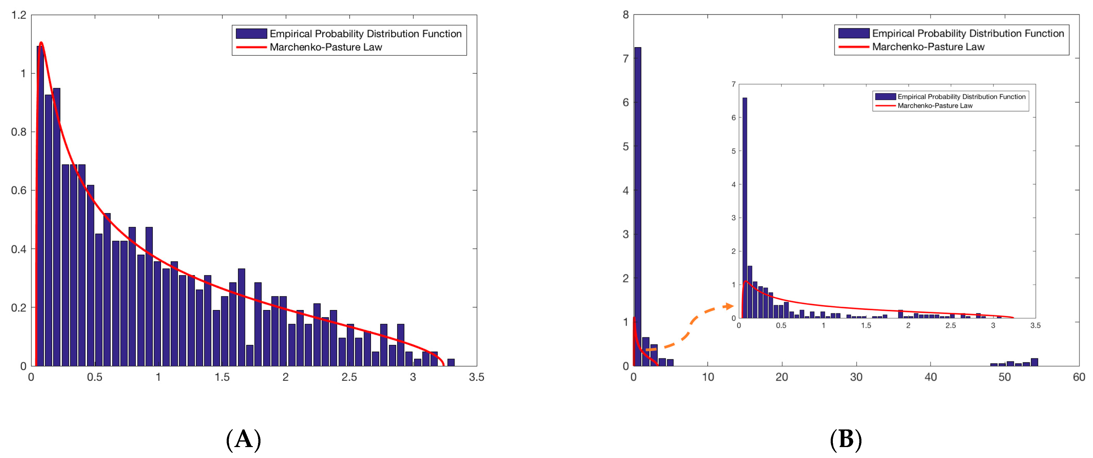
6], implying that their tasks change over time. This time interval can be divided into thousands of non-overlapping stationary windows. In this manner, we obtained a set of thousands of matrices. The application of eigenvalues to express features in EEG data has a long history, particularly in relation to the random matrix, which makes the fluctuations in eigenvalues somewhat interpretable [7].

1.1. Related Works

Of all the clinical manifestations of mental disorders, schizophrenia is the most complex. The severity of schizophrenia is reflected in the complexity of its symptoms. This paper explores EEG data with the aim of finding an effective method by which to diagnose and discriminate between the diverse clinical manifestations of individuals with schizophrenia. Many methods have been developed to understand EEG characteristics in terms of schizophrenia. Early traditional methods have relied on experienced doctors to observe EEG data and provide clinical diagnostic results based on their experience [8]. However, different doctor make different judgments that are influenced by many factors, such as their understanding of the pathogeny and the patients, and even their personal emotions. Schizophrenia has been hypothesized to be a brain connectivity disorder that results from abnormal structural and functional connectivity networks [9]. Maran indicated that such abnormalities exist within functional connectivity in resting-state and task-related EEG data [10]. Statistical methods can be used to detect and visualize brain function dynamics and complexity, so as to then identify abnormal mental disorders [11]. Conventional univariate statistical methods neglect the highly interrelated nature of the functional and structural aspects of the brain data, as well as the difficulties in dealing with large amounts of EEG data. Choosing the appropriate feature extraction for schizophrenia diagnosis is a challenging task that requires extensive knowledge of signal processing and artificial intelligence.
Machine learning algorithms have been used to diagnose schizophrenia using EEG data. Extensive research has shown that traditional classifiers, such as support vector machines (SVM) [12], K nearest neighbors (KNN) [13], Naive Bayes [14], decision trees [15], and random forests [16], are already being used. With the rapid development of artificial intelligence technology, although the classification accuracy of these methods is sufficient enough to provide a clinical reference, their generalization ability needs to be improved. A convolutional neural network (CNN) was used to classify EEG-derived brain connectivity in schizophrenia [17], which achieved a remarkable accuracy of 93.06% with decision-level fusion. The high accuracy achieved by the CNN could be attributed to its ability in terms of end-to-end learning and utilizing hierarchical structures between data [18]. Deep learning is also used for identifying individuals with schizophrenia through applying a CNN to capture the unique physical features of resting-state EEG data, reaching a good degree of accuracy at 88% [19]. However, these works lacked interpretability for clinical applications.
Many classical statistical methods induce large, sometimes intolerable, errors. It is important to develop new approaches to deal with high-dimensional data [20]. Random matrix theory (RMT) is a very appropriate candidate model, since the classification methods based on RMT rely on singular values of a large-dimension random matrix. RMT originated in physics and is naturally composed by sampling sequences of multiple random variables [21]. Under some assumption, the eigenvalues or singular values distribution of RMT, spectral statistics, is estimated by the regular form or upper and lower bounds [22]. For instance, early research on random matrices XN×T, where N stands for the number of multivariates and T refers to the sampling length, was introduced when the Chi-square distribution was extended to multivariate random data. If we assume that each dimension of random data is i.i.d. with a mean of zero, XXT is a p-order symmetric matrix that follows the Wishart distribution. In 1967, Marchenko and Pastur conducted a study of matrices of the order XTX. When N is sufficiently large and all variables follow an independent, identically distributed normal distribution variable, its eigenvalue density distribution converges to follow the Marchenko Pastur law [23]. Today, it is a perspective method widely applied in financial analysis, physics, biological statistics, and computer sciences [24].
However, each variable does not follow a normal distribution or other standardized distribution assumptions, singular values of X, or, in other words, the eigenvalues of its covariance matrix of X are not sufficiently regular as statistical features of multiple random variables. A linear eigenvalues statistic (LES) of X and LES-associated appropriate test functions can be used to identify the statistical features of the multivariate random matrices X. Musco provided the theoretical upper and lower bounds of LES with respect to different test functions; for example, the log-determinant, the trace inverse, and the Schatten p-norms [25]. By introducing a more general assumption of the multivariate variance distribution, the existing bounds of linear eigenvalue statistics for random matrix ensemble were re-established [26]. For testing the additive effect of the expected familial relatedness, according to a dataset from the UK Biobank, a study was conducted based on LES [27] where the four test statistics, the likelihood ratio test (LRT), the restricted likelihood ratio test (RLRT), and the sequence kernel association test (SKAT) statistics were employed. For ozone measurements, Han proposed an LES statistical estimation in which the LES-associated test function included a log-determinant, the trace of the matrix inverse, the Estrada index, and the Schatten p-norm to estimate over 6 million variables [28]. Four test functions were used for anomaly detection in the IEEE 118-bus system, including LRT and Chebyshev Polynomials [29]. However, there are still very limited applications of RMT in neuroscience. The adoption of RMT in studying EEG data in this research is driven by its ability to provide insights into the statistical properties, noise characteristics, and universal features of the data.
In summary, we can conclude that the different test functions of LES for the same random matrix X have different classification performances. The questions are: which test function is best? Or, how do we find a better one?
In additional, when using EEG data to diagnose schizophrenia, the methods mentioned above focus on the binary classification of FES and HC. Thus far, very little attention has been paid to the role of ternary classifications with the addition of CHR. Distinguishing CHR from HC and FES and preventing the development of CHR in its prodromal stage plays a critical role in treating schizophrenia.
In this paper, we employed LES statistical characteristics, a nonlinear law established for random multivariate, to diagnose schizophrenia, and studied the most appropriate test functions to identify the statistical features of X derived from multivariate random matrices.

1.2. Our Contributions

This study proposes a deep learning method, LES-NN, in which a sequence of LES is the input of a successive deep learning neural network to identify a patient’s mental status in schizophrenia research. The statistical performance of the LES relies on the test function. However, the optimal statistical test function is a functional optimization problem. The proposed LES-based deep learning neural network method involves an iterative learning procedure for the proposed test function optimization problem coupled with the successive parameter optimization of a neural network.
First, EEG data can be divided into matrices, then, the data feature can be characterized using the RMT, within which LES designs are systematically studied. LES is a high-dimensional statistical indicator with different test functions. LES gains insight into systems from different perspectives. In addition, by exploring suitable test functions within the existing functions with physical and statistical significance, it can be found that entropy performs well as a test function for classifying EEG data.
Furthermore, to determine an optimal statistical test function, a functional optimization problem is proposed that relies on the final precision of the model’s output. Finally, we introduce an LES-based deep learning neural network model that synchronously couples the proposed statistical test function functional optimum problem and NN evolution to simultaneously determine the optimal form of the test function and NN parameters. The proposed LES-NN method achieves excellent results for HC, FES, and CHR classification problems. By delving into different instances of schizophrenia, we aim to offer valuable insights into its diagnosis and management.
The paper is organized as follows: The first section includes an introduction to EEG with the prodromal phase of schizophrenia and a learning algorithm with RMT. The second section provides a general overview of the EEG data sources and preprocessing. Section 3 describes the fundamentals of a RMT and LES. Section 4 presents the design of the LES test function with machine learning and deep learning neural networks. Finally, the results, discussion, and conclusion are presented in Section 5 and Section 6.

2. Data Source and Preprocessing

This study aimed to investigate classification issues with resting-state EEG by evaluating three types of participants: high-risk (CHR) individuals, clinically stable first-episode patients with schizophrenia (FES), and healthy controls (HC). Our study included 120 participants (40 CHRs, 40 FESs, and 40 HCs), and 80% of all these data were used as training sets and 20% were used as test sets. The participants investigated in this study were recruited from a mental health center hospital in Shanghai, and all participants signed informed consent forms to participate in the study. Continuous EEG activity was recorded while the participants were comfortably seated with their eyes closed. The EEG recordings were placed between 09.00 and 17.00. The participants were monitored for electroencephalographic signs of somnolence for the entire recording duration (5 min). Recordings were conducted using 64-channel Ag/AgCl electrodes (two reference electrodes, M1 and M2) arranged according to a modified 10/20 system at a sampling rate of 1 kHz. Electrode impedance was kept below 5 Ω. As the raw EEG signal was contaminated with noise and artifacts of external and physiological origin, a 0.1–50 Hz band-pass filter and automatic artifact rejection based on ICA were applied offline to remove power-line interference, ocular artifacts (EOG), and muscle tension. The spatial positions of the EEG sensors are shown in Figure 1A. And the EEG data are illustrated in Figure 1B.
Let N be the numbers of channel electrodes and T be the sample size. The EEG sampling can be denoted as a N × T matrix X. Let W be the sliding window size and L be the windows number, that is L = T/W. Then, the sample time series data X is divided into a sequence of random matrix: X = (∑1, ∑2, ⋯, ∑L−1, ∑L) as shown in Figure 2. Here, each ∑i is N × W dimensional.
One advantage of data blocking is to avoid the problem of non-stationary data, as EEG data are non-stationary signals. The EEG data were blocked and assumed to be stable within each block. However, we tried to turn big EEG data into tiny data for practical use, and some recently advanced data-driven estimators could be adopted to obtain state evaluation without knowledge of medical parameters or connectivity [30]. Considering that the characteristic of the data is an extremely long time series, this study illustrates the conceptual representation of the structure of the massive streaming EEG data.
We can obtain a data matrix for each block Σ i , which are in a high-dimensional space but not infinite; more explicitly, we take a finite-dimensional parameter optimization problem in a tensor space according to the universality theory [31] of RMT for a real-world system.

3. Fundamentals of Random Matrix Theory

3.1. Large-Dimensional Data and Random Matrix

In multivariate statistics, we obtain a W sampling of N-dimensional random vectors: x 1 , x 2 , , x L     R N . We then form the data matrix X = x 1 , , x L R N × W , which, naturally, is a random matrix that needs high-dimensional data analysis. Remarkably, N and W were large and comparable. The classical “large W, fixed N” theory fails to provide useful predictions for many of these applications. Classical methods can be significantly broken down into high-dimensional regimes. The possibility of an arbitrary sample size N renders classical statistical tools infeasible. We consider the asymptotic regime to be
N , W , b u t N W c 0 ,
Compared with traditional probability theory, a random matrix is defined as a random variable for the elements of the matrix. Given an N × N Hermitian matrix AN, let λ1, λ2, ⋯, λN be eigenvalues of AN. If the eigenvalues λi of AN are real, we can define a one-dimensional empirical spectral distribution function (ESD) as
F A N x = 1 N 1 i N : λ i A N x = 1 N i = 1 N I λ i A N x ,
The main task of RMT is to study the limit properties of F A N when AN is random, and the order n tends to infinity. If F A N has a limit distribution, then we call this limit the limiting spectral distribution (LSD) of the matrix AN. Currently, two main research methods are used to determine the limit properties of F A N : the moment estimation method and the Stieltjes transformation. The convergence rate from the ESDs of a large-dimensional random matrix to its corresponding LSD is very important for applying RMT. The best-known convergence rate for the expected ESD of the Wigner matrix and sampling covariance matrix is O(N−1/2), and the corresponding ESDs are O(N−2/5) and O(N−2/5+η) [32].

3.2. Marchenko-Pastur Law

There are various types of random matrix models, with the Gaussian unitary ensemble (GUE) and the Laguerre unitary ensemble (LUE) being the most common [33]. The LUE can be a rectangular matrix that comes closer to real-world data and has a wider range of applications. Therefore, this study adopts a sample covariance matrix for data modeling.
Consider a sample covariance matrix of the form.
S N = N 1 X X H
where X is a matrix whose entries X j k j = 1 , , N ; k = 1 , , T are independent random variables satisfying the following conditions [34].
E X j k = 0 , E X j k 2 = 1
Let λ j j = 1 N be the eigenvalue of SN. The RMT deals with the statistical properties of the eigenvalues λj of the sample covariance matrix SN
S N λ j = λ j λ j
where | λ j represents the sample covariance matrix corresponding eigenvectors. The simplest property of the eigenvalue family related to a matrix ensemble is the eigenvalue density ρ λ . This counts the mean number of eigenvalues contained in intervals (a, b).
λ j ; λ j a , b = a b ρ λ d λ j ; λ j a , b = a b ρ λ d λ
According to the above distribution entries of matrix X, we obtain an ensemble of random matrices, which Marchenko and Pastur mathematically studied. In particular, the density ρ λ of the ensemble is known and given by the formula, if c ≤ 1, the density of which is given by [35]:
ρ c λ = 1 2 π c λ b λ λ a w h e r e , a = 1 c 2 , b = 1 + c 2
The Marchenko-Pastur law is an analog of Wigner’s Semicircle law in this setting of multiplicative rather than additive symmetrization, and the assumption of Gaussian entries may be significantly relaxed.

3.3. Feasibility for Modoling EEG Data in RMT

According to the definition of spectral density, the data must be independent. Since EEG is not a random signal, it is synchronous and related to the corresponding brain activity. We can expect that the spectral density does not follow the prediction of the Marchenko-Pastur law and is related to human activities. Fortunately, the real EEG data are not completely inconsistent with this spectral distribution. The results are shown in Figure 3. We randomly chose the data frame from one object because these three groups of data show an approximate result to keep the results simple to comprehend.
The blue bar in Figure 3 A represents the empirical spectral distribution of the eigenvalues of N−1XXH, and the red curve represents the Marchenko-Pastur law with a density function. There were some differences between the actual and simulated data. In Figure 3B, at the head of the distribution, there are a certain number of eigenvalues near zero. At the tail of the distribution, several large eigenvalues are outliers. When we magnify the empirical spectral distribution of the eigenvalues (blue bar) below the spectral distribution limit (Marchenko-Pastur law, red curve), we are surprised to find that the distribution of the empirical and limit of this part coincides to a certain extent. According to the definition of the random matrix, the part below the Marchenko-Pastur law shows that the data conform to the characteristics of random noise, named “noise subspace”. However, the noise subspace here does not fully fit the theoretical value because this part contains a few parts of the information. Other parts, including the eigenvalues near zero and outliers, show information about the data, named “signal subspace”. Eigenvalues near zero indicate a correlation between the data and actual activities that can affect outliers. A test statistic that embodies the characteristics of all the eigenvalues should be adopted to derive profound and subject-independent information from EEG data.

3.4. Linear Eigenvalue Statistics

Definition 1. 
Since the pioneering work of Wigner [36], it has been known that if we consider the linear eigenvalue statistic of the random matrix corresponding to any continuous test function  φ .
L E S X ( φ ) = j = 1 N φ λ j
The law of large numbers is an important step in studying eigenvalue distributions for a certain random matrix ensemble. Then,  N 1 L E S X ( φ )  converges in probability to the limit [37]:
l i m N N 1 L E S X ( φ ) = φ λ ρ λ d
where  ρ λ  is the probability density function (PDF) of the eigenvalues.
Similarly, different test functions can be designed to obtain diverse LES as indicators and theoretical values. The classical test functions are listed in Table 1.
An appropriate form of the LES test function could be a feature for classification among different schizophrenia states.

4. Methods

4.1. LES-Based Algorithm Frameworks

The EEG data obtained from the experiments were analyzed using machine learning and deep learning models. Here, we focused on the random matrix and its linear eigenvalue statistics. We developed traditional machine learning algorithms and deep learning networks to obtain the baseline classification performance and compared them with a proposal LES-based deep learning neural network model. The benefits of traditional machine learning and deep learning approaches depend more on the data itself; however, there is no clear statistical or physical significance. The construction of the LES-based deep learning approaches conforms to the definition of LES, which attempts to construct appropriate test functions for the spectrum of data matrices and has certain physical and statistical significance. In this paper, we propose a LES-based deep learning network scheme in which a LES series of the random matrixes, consisting of EEG data sliding window sampling, is employed as a feature preprocessing layer for the learning network. Due to the performance of LES-based scheme being too sensitive to choose the LES’s test function. The proposed LES-based deep learning network has two types of combination of LES test functions and learning techniques: the first type is the LES’s test function selected (shown in Figure 4A); while the second type is the optimal LES’s test function that should be solved in a functional optimization problem (shown in Figure 4B).
Data preprocessing was previously explained in the paper, and the remaining structure and functions of each block diagram are explained in the following sub-sections. The calculating LES-related processes are shown in Algorithm 1.
Algorithm 1: EEG data classification with LES features using machine learning and deep learning.
Input: Raw EEG data matrix X is a N × T dimensional, which is time series data of N dimensions within the T sampling period
Output: a binary or ternary classification result.
1:
large EEG data are cut into suitable data blocks, according to Figure 2, and sliding windows of size W, X = (∑1, ∑2, ⋯, ∑L−1, ∑L)
2:
for each sample matrix, X = Σ i  do
3:
Standardization: all entries satisfying the conditions E X j k N = 0 , E X j k N 2 = 1
4:
Obtaining a sample covariance matrix of matrix X of the form S = N 1 X X H
5:
Calculating eigenvalues λ i   o f   X ;
6:
end for
7:
Selecting or learning the appropriate test function φ to calculate LES as the feature ζ i , 1 i L ; and ζ 1 , ζ 2 , , ζ L are input in classification algorithms.

4.2. Machine Learning Scheme with LES in Selected Test Functions

Values or attributes with information meanings extracted from raw data constitute the input of the machine-learning model, and they generate prediction results through various classic models. The LES test functions as a feature that can reduce the number of features and dimensionality to enhance the model’s generalization ability.

4.2.1. Feature Extraction

The main feature extraction task is to derive salient features that map the EEG data into different states. Feature extraction is related to dimensionality reduction techniques when the input data to an algorithm are too large to be processed and are suspected to be redundant. It is fundamental to study the spectral analysis of a large-dimensional random matrix that concerns the central limit theory of the LES. This is because many important statistics in multivariate statistical analyses can be expressed as functions of the empirical spectral distribution of a random matrix. The sample covariance matrix and LES (a kind of dimensionality reduction LES) are parts of feature extraction because we are concerned with mapping eigenvalues.
The LES in this study represents a function, which involves reducing the resources required to statistically describe a large set of EEG data. When studying LES, the test function is usually required to satisfy certain strong regularity conditions with the eigenvalue of a random matrix.

4.2.2. State Classification

The computed features are then fed into the classifier for classification between the different states of the human brain. The following classifiers are used in this study: support vector machines (SVM) are considered the best state-of-the-art classifiers with lower complexity than other classifiers. SVM is based on finding a hyperplane that can classify data into separate classes with the possibility of a maximum margin. K-nearest neighbor (KNN) is a classification algorithm based on supervised learning that is suitable for classifying class domains with large sample sizes. Naive Bayes is based on Bayes’ theory and assumes that each attribute of a given class is independent of the values of the other attributes. However, a decision tree is a top-down recursive construction method. The decision tree is a typical classification method that approximates the value of a discrete function. Random Forest is a random method to build a forest with many decision trees, and there is no covariance between each decision tree.

4.3. LES-Based Deep Learning Network Scheme

In this section, we describe the proposal LES-based deep learning network scheme in detail. The performance of the proposal LES coupling deep learning neural network classification algorithm was based on LES fluctuations in sample covariance random matrices. According to its definition, the LES relies on the test function. This method has good physical and statistical significance, and the LES-based DNN aims to learn a better form of the test function.
We need to construct a suitable statistical test function related to the Random Matrix of the sample information to reflect the information of the overall data and better describe the latent information; more clearly, this latent information is relative to those network parameters of the successive deep learning neural network. In the proposal LES-based deep learning neural network scheme, the test function functional optimization problem and the deep learning network are coupled to be synchronously optimized during the training process.
The joint optimization problem of the LES-based DNN in training is shown as follows:
m i n   φ , θ J L E S X ( φ ) , θ
Here, φ L [ 0 , + ) . The integrable function space;
θ refers to all weight coefficients of the adopted deep neural network in the proposal LES-based DNN method.
J L E S X ( φ ) , θ is the objective of the joint optimization problem, i.e., the loss function of the LES-based DNN, as shown in Figure 5.
In the training process of using deep neural networks and optimization theory, we reformulated the mathematical model to an optimization problem with variables as functions.
According to (10), an optimal test function associated with EEG data is a functional optimal problem in integrable function space L [ 0 , + ) . We know that finding an optimal function in an infinite-dimensional space is an extremely difficult task.
Furthermore, in this paper, we propose a finite-dimensional parameter optimization problem in tensor space to narrow the search space.
Let us suppose that the tensor space is based on a set of basic kernel functions φ i i = 1 n .
Hence, this means that the candidate test functions are confined to combinations of basic functions, as follows:
φ α i = 1 n α i φ i , h e r e α = [ α 1 , , α n ] , α i R
The joint optimization problem LES-based DNN in training is revised as follows:
m i n   α , θ J L E S X φ α , θ
Here, α refers to the tensor coefficients of the basis kernel φ i i = 1 n .
How to choose suitable basis functions φ i i = 1 n is thought as a technique; for example, the candidate basis functions is so that the test function in (10) cover the traditional ones in Table 1.
J L E S X φ α , θ is the objective of the joint optimization problem, i.e., the loss function of the LES-NN, which is composed of cross-entropy and the regular term shown the in following (13). In which the cross-entropy denoted as J0 could measure the difference between the learned model distribution and the real data distribution; the regular term, β Ω θ , here Ω, is the L2 norm regularization term, which limits the learning ability of the adopted deep neural network and prevents parameter overfitting; β is the proportion hyperparameter. The sum of the squares of all coefficients includes the tensor coefficients and LES-NN weight coefficients divided by m, which is the number of samples in the training set.
J = J 0 L E S X φ α , θ + β Ω L E S X φ α , θ J 0 ( L E S X φ α , θ = 1 N i = 1 N y i ( L E S X φ α , θ ) l o g p i + 1 y i ( L E S X φ α , θ l o g 1 p i Ω ( L E S X φ α , θ = 1 2 m α , θ 2

4.3.1. Optimal Test Function and LES

Determining the optimal statistical test function is a functional optimum problem in the space of continuous functions. In most practical applications, it is difficult for the target variable to have a linear relationship with the input variable; therefore, we attempted to use a more general polynomial function for fitting. When the power function of the variables is used for a linear combination, the fitting effect is better for many non-linear practical applications. We introduced other forms of non-linear functions to increase the fitting effect.
Once the base kernel function is designed, it is first necessary to determine the tensor coefficient α. Here, we introduced an LES-based neural network model that couples the proposed statistical test function functional optimum problem with the network parameter training. Referring to the definition of LES (8), the 1 × 1 convolutional kernel can change the size of the channel dimension, similar to compressed sensing. Therefore, we were inspired to use the 1 × 1 convolutional kernel to implement networks that satisfied the LES definition. Thus, tensor coefficient optimization can be incorporated into deep neural networks.

4.3.2. The Proposed LES-Based Neural Network

Brain signals are complex, and directly analyzing the raw data of the entire brain using neural networks requires a large amount of computation. By compressing and perceiving raw data through LES, analyzing only the eigenvalues of the EEG data can effectively reduce the computational complexity. We developed a novel neural network that strictly satisfied the definition of LES. We used a 1 × 1 convolutional kernel to realize LES features, which were then integrated for classification decisions to discriminate schizophrenia and HC with or without CHR. The specific characteristics of each part of the LES neural network are shown in Figure 5. The detailed procedure is as follows.
First, we standardized the normal distribution of the eigenvalues of the sample covariance matrix of each EEG data block as input; the standardization coefficient was 1 / n . The dimensions of the input data to the deep learning model were an N × L eigenvalue matrix, where N is the number of EEG channels and eigenvalues of the sample covariance matrices, and L is the number of time blocks. The core structure of the deep-learning model is the LES layer, which introduces the concept of obtaining high-dimensional feature information using random matrices.
Secondly, we designed the network structure of the layer to learn the LES feature. The feature fusion and test function were realized by contacting the eigenvalues with a 1 × 1 convolution kernel, which could be seen as special, fully connected layers. This layer rearranges and combines the connected features to form an LES. It can significantly increase the non-linear characteristics (using the following non-linear activation function) while keeping the scale of the kernels/feature maps unchanged. It can achieve cross-channel interactions and information integration with linear correction characteristics and a linear combination of multiple kernels and feature maps. The operation mentioned above is an on a channel that linearly combines the dimensions of the channels, which naturally conforms to the definition of the LES test function. This study designed a 1 × 1 convolutional kernel layer, where the former is n × 1 × 1, linearly combine data on different channels, and then perform non-linear operations that can achieve dimensionality down functions. The parameters of different channels are the tensor coefficients of the basis kernel α = [ α 1 , , α n ] . Different sets of linear projections that can be separately learned can be used to discuss the impact of the linear combinations of several LES kernels on the results. We also discuss the impact of different LES kernels on the results based on the weight of each LES kernel.
Finally, the features obtained from the learned test functions are sent to a multilayer perceptron to realize the classification algorithm.

5. Cases and Discussion

We constructed a training set and test set from raw EEG data to perform a more reliable classification process, and the cross-validation method is presented in this study. The training set consisted of 80% samples that were randomly selected from raw data, while the remaining part of the test set first used the training set to train the classifier and then used the test set to validate the trained model; this process was repeated several times to obtain statistical information of the observations. Therefore, it is the performance index of the classifier. As previously mentioned, several classification methods were adopted in this study, as shown in Figure 4. The purpose of these cases was to classify CHR based on the algorithm’s ability to distinguish HC and FES well. For learning algorithms, this is the problem of binary and ternary classification, so we use the notation “HC/FES” and “HC/FES/CHR” to represent these two classification problems.

5.1. Machine Learning with/without LES in Selected Test Function

5.1.1. Comparison of Various Extracted Features

Feature extraction is extremely important because it seeks to reduce the dimensionality of the data synthesized as a feature vector, preserving and highlighting useful information from raw data. The quality of feature selection directly affects the success rate of classification. The computational effort required and the balance between success and efficiency should be considered.
Statistical features summarize the windows in a global view of the data [38] and can be analyzed as follows Table 2.
The characteristics of each electrode during the sampling period were obtained using these statistical features. There were sixty-two electrodes in total; each electrode could obtain seven statistical features, and we obtained 62 × 7 features. These features are trained using a variety of machine-learning methods.
Table 3 shows the classification performance of classifiers under several statistical features in distinguishing between two or three types of schizophrenia states. It can be observed that the binary classification problem between HC and FES has a good classification effect; the accuracy of each classifier is greater than 70%, particularly when that of the SVM method is close to 80%. One important aspect here is that the SVM classifier has three types of kernels, namely linear, polynomial, and RBF, and we chose the RBF kernel to obtain the results in this study. We have already conducted a sample comparative experiment among these kernels, proving the RBF’s robustness over the polynomial and linear for these datasets; therefore, the SVM with the RBF kernel was chosen as the basic kernel in the remaining paper.
However, when the third state (CHR) is placed in the classifier, the accuracy worsens, and the success rate is only approximately 60%. This means the feature extraction method cannot accurately distinguish with the third state. A result of <70% has no reference value for clinical applications.

5.1.2. Effect of Machine Learning with LES in Selected Test Function

This section roughly represents EEG data in terms of high-dimensional data vectors; geometrically, there are points in a high-dimensional vector space. Here, random variables are simultaneously, spatially, and temporally taken into account. The central idea is to treat the vectors as a whole rather than multiple samples of random vectors. According to Algorithm 1, we tried to turn raw EEG data into many tiny data blocks, and each block calculates the LES feature based on some test function. We used the concept in Section 3.3 to show several popular test functions in Table 1.
Different classifiers and features (LES) were selected for the experiments, and the classification results were compared and analyzed. For the results shown in Table 3, it is worth noting that the result of LES feature extraction is better than traditional statistical feature extraction by approximately 10%. The highest classification accuracy is approximately 90% in binary classifications and approximately 70% in ternary classifications, which is very encouraging. It can be seen that the performance of the classifiers used was satisfactory in distinguishing between HC and FES, and using von Neumann Entropy as an LES test function combined with the SVM classifier could obtain the average classification accuracy of 73.31% during ternary classifications among HC, FES, and CHR. Compared with the results in Table 3, the binary classification results between HC and FES could relatively easily obtain good results, and a classification success rate higher than 70% could be used to assist clinical diagnosis; different from statistical features based on LES.
If the training set is small, high-bias/low-variance classifiers (e.g., Naive Bayes) have an advantage over low-bias/high-variance classifiers (e.g., kNN) because the latter will overfit. However, low-bias/high-variance classifiers start to win out as the training set grows (they have a lower asymptotic error) because high-bias classifiers are not powerful enough to provide accurate models. However, better data often outperform better algorithms, and designing good features is challenging. If you have a large dataset, the choice of classification algorithm might not matter in terms of classification performance. The datasets used in this study are large but not large enough to ignore the differences between various classification methods; in other words, the differences between the various classification methods are not significant, but the differences cannot be ignored.
According to Table 4, under the same feature selection, the results of the SVM were better than those of the other classifications. It is obvious that the advantages of SVM are high accuracy, good theoretical guarantees regarding overfitting, and an appropriate kernel; it can work well even if the data are not linearly separable in the base feature space, which is especially popular in classification problems where high-dimensional spaces are the norm. Various test functions are of central importance in RMT. Several popular statistical indicators were used as test functions in this study, each with its engineering interpretation; the significance of selecting the test function is that it can give a mathematical meaning to LES. The von Neumann Entropy performance yielded the best results using the machine learning method compared to the other functions.

5.1.3. Effect of Different Block Window Sizes in the LES Feature

Previously, we used a fixed sampling period as the sampling base to perform identification and obtained good classification results. In this section, we sought to find another sample time length of the EEG signal that could still preserve the identification information, and we compared their performance differences. We divided each EEG signal sampling point into portions (W from 100 to 5000) and performed the same procedure. The von Neumann Entropy was used as the test function based on the results of the above comparative experiments, and SVM was selected for classification.
The classification results are listed in Table 5. From the table, we can observe that as the length of the sample size increases, different W values affect the estimation accuracy of the sample covariance matrix, and the maximum classification accuracy is located at W = 200. In classical statistics, the sample size is usually three–eight times the dimension, which means the suitable range of W should be from 100 to 1000. The results show that the sample size over which the participants could be individualized was approximately 200.

5.2. Effect of Proposed LES-Based Deep Neural Network

Different test functions significantly impact the classification results. In this section, based on the linear combination of different kernels, such as φ i i = 1 5 and φ i i = 1 10 , the EEG data were trained and tested, and ten-fold cross-validation was conducted. In addition, in light of the results of different window size effects, W = 500 was chosen.
According to the above design principles, several base kernel functions were extracted and derived from Table 1, as well as other polynomials including higher-order terms of variables and exponential terms, the base kernel function in this paper is:
φ 1 = x , φ 2 = x , φ 3 = x 2 , φ 4 = l o g x , φ 5 = x l o g x φ 6 = x 3 , φ 7 = x 4 , φ 8 = l o g 1 + x , φ 9 = 1 1 x , φ 10 = e x
The weights of each kernel of the different classifiers are summarized in Table 6; owing to the constraint of weight decay, the weight values presented in the table are not abnormally large. In the classifier of the five kernels, x and x l o g x played larger roles. This result also agrees with the results of the manual selection mentioned earlier. However, in the classifier of the 10 kernels, the results of each weight became more averaged and did not significantly reflect a particular kernel, which requires further excavation. Their physical and statistical significance may partly explain these relationships between different weights. Exploring the significance of these weights can enhance the interpretability of classification models, and further analysis and research on CHR data can be conducted in conjunction with clinical conversion experiments.
The results obtained from the LES-based deep learning model for EEG data classification are presented in Table 7 and Figure 6. We compared the performance of the deep learning model with that of the machine learning model, and the results showed that the LES-based deep learning model had fairly high accuracy in classification using features derived from a linear combination of test functions. The most striking observation from the data comparison was that with five kernels or ten kernels as the classifier, the accuracy of the binary classification results exceeded 90%, and the result with ten kernels was near 90%. No significant differences were observed between the two conditions (linear combinations of different kernels). The binary classification accuracy of the five kernels was lower than that of the ten kernels, and the ternary classification results for the ten kernels were better. This may be related to the amount of data used in this study, but there is also the problem of generalization. Further studies should use more data to validate and improve these results.

5.3. Discussion

Since the exceptional performance of CNN-based ImageNet dataset applications has significantly grown. In order to compare the LES-based algorithm with other traditional deep learning algorithm, such as end-to-end CNNs, we evaluate the effectiveness of the CNN at the end of this paper.
In accordance with the preprocessing procedures outlined in Section 4.1, this study implemented noise reduction techniques, including filtering, the removal of artefacts, and data segmentation. Additionally, EEG data were normalized to fit the input requirements of the convolutional neural network. Based on forward and back propagation algorithms used in convolutional neural networks, we used AlexNet as a template to construct a basic CNN, including a convolutional layer, a pooling layer, activation function, a fully connected layer, a softmax layer, and a dropout unit. We provided a concise overview of the deep convolutional neural network methodology used in this section, as demonstrated in Table 8.
Table 9 shows the classification performance of the CNN. Whilst the CNN was unable to outperform the combination of SVM and LES on the binary classification problem, it significantly outperformed them on the ternary classification problem. Filtering a signal is the basic principle of convolution, and it excludes subjective evaluations unless clearly marked as such, filtering out information that may be of interest or usefulness to us. However, it lacks sensitivity to the overall position of characteristics and disregards the interdependence of features in the data. Although it does not show enough advantages in the binary classification problem, it gives us confidence in the ternary classification problem to design a more appropriate network that can have some interpretability while getting better results, such as the LES neural network.
We also calculated the computational time required for the proposed LES-based deep learning network to classify the EEG data features of the individual participants. The classification algorithm was implemented using an Intel(R) Core(TM) i7-13700H GPU (Lenovo’s computer manufactured in Beijing, China) on an NVIDIA GeForce RTX 3080 Ti with 10 GB of VRAM on 64-bit Windows 10 Professional. Calculating the eigenvalue of the data covariance matrix is performed during preprocessing, which reduces the number of parameters input into the model nearly hundreds of times and improves robustness to data noise. We can easily simultaneously load all the data into the memory, which also improves the computational efficiency of the training. Based on these results, the training time of the LES-NN was no more than 5 min when the loss of the model converged to a low level, and the testing time of each participant was only 20 ms.

6. Conclusions

In the classification diagnosis of schizophrenia, it is crucial to accurately and timely screen for and intervene in CHR. However, the diagnosis of CHR is challenging. In this study, we identified a large amount of EEG data in patients with schizophrenia (including FES and CHR) compared to HC. Randomness and uncertainty are the key characteristics of these data. RMT and LES provides an influential mathematical framework for exploring statistical properties of complex systems, such as EEG signals. In a random matrix X = x 1 , , x T R N × T , we used N nodes to represent the sample size and T data samples to represent the temporal samples. When N and T are large, a special mathematical phenomenon called concentration occurs, which provides powerful theoretical support based on RMT for processing EEG data.
We introduced LES from RMT as a feature, which reflects the fluctuation of the central limit theorem of the origin data and has good physical and statistical significance. This LES-based statistic applies to machine learning and deep learning analysis methods. This study analyzed several classic functions as test functions and combined them with various machine learning algorithms, such as SVM, KNN, Random Forest, etc., to obtain results that meet the requirements of clinical auxiliary diagnosis.
Furthermore, a deep learning network model that satisfied the mathematical definition and properties of LES was designed, and the optimal form of the LES test function was explored, resulting in better results than machine learning methods. The LES-based network focuses on the spectrum of the data matrix, and after preprocessing, there are fewer network parameters, which can improve the training efficiency. Adding CHR to the ternary schizophrenia classification results achieved a classification accuracy of nearly 90%. As different test functions have different physical and statistical meanings, test functions can be employed to meet the needs of clinical experiments to make the algorithm more interpretable, this result could potentially change the current ways of diagnosing and treating schizophrenia. The increased precision means physicians could make more accurate diagnoses of patients and consequently devise more personalized and effective treatment plans. The role of LES-based indicators in informing clinical interventions will be explored in our further research, for instance, making use of EEG microstate analysis to guide intervention plans.
This prospective work on time-domain signal analysis of EEG data included data analysis based on the spatiotemporal representation information of EEG signals. Therefore, we will introduce a more suitable model to solve this problem in future research.

Author Contributions

All authors made a significant contribution to the work reported, whether that is in the conception, study design, execution, acquisition of data, analysis and interpretation, or in all these areas; took part in drafting, revising or critically reviewing the article; gave final approval of the version to be published; have agreed on the journal to which the article has been submitted; and agree to be accountable for all aspects of the work. All authors have read and agreed to the published version of the manuscript.

Funding

This work was supported in part by the China National Research and Development Key Research Program under Grant 2020YFB1711204 and Grant 2019YFB1705700.

Data Availability Statement

The data presented in this study are available on request from the corresponding author. The data are not publicly available due to the researcher and the institution providing the data have signed relevant confidentiality agreements.

Acknowledgments

We are appreciated for department of EEG source imaging leaded by Jijun Wang from SHJC for data providing and discussion. We also grateful to Tianhong Zhang from SHJC for his expert collaboration on data analysis.

Conflicts of Interest

The authors declare no conflict of interest.

References

  1. Zhang, T.H.; Tang, X.C.; Li, H.J.; Woodberry, K.A.; Kline, E.R.; Xu, L.H.; Cui, H.R.; Tang, Y.Y.; Wei, Y.Y.; Li, C.; et al. Clinical Subtypes That Predict Conversion to Psychosis: A Canonical Correlation Analysis Study from the ShangHai At Risk for Psychosis Program. Aust. N. Z. J. Psychiatry 2020, 54, 482–495. [Google Scholar] [CrossRef] [PubMed]
  2. Cincotti, F.; Mattia, D.; Aloise, F.; Bufalari, S.; Astolfi, L.; Fallani, F.D.V.; Tocci, A.; Bianchi, L.; Marciani, M.G.; Gao, S. High-Resolution EEG Techniques for Brain–Computer Interface Applications. J. Neurosci. Methods 2008, 167, 31–42. [Google Scholar] [CrossRef] [PubMed]
  3. Fouad, M.M.; Amin, K.M.; Elbendary, N.; Hassanien, A.E. Brain Computer Interface: A Review. Intell. Syst. Ref. Libr. 2015, 74, 3–30. [Google Scholar] [CrossRef]
  4. Roy, Y.; Banville, H.; Albuquerque, I.; Gramfort, A.; Faubert, J. Deep Learning-Based Electroencephalography Analysis: A Systematic Review. J. Neural Eng. 2019, 16, 051001. [Google Scholar] [CrossRef] [PubMed]
  5. Wang, X.W.; Nie, D.; Lu, B.L. Emotional State Classification from EEG Data Using Machine Learning Approach. Neurocomputing 2014, 129, 94–106. [Google Scholar] [CrossRef]
  6. Gramfort, A.; Strohmeier, D.; Haueisen, J.; Hmlinen, M.S.; Kowalski, M. Time-Frequency Mixed-Norm Estimates: Sparse M/EEG Imaging with Non-Stationary Source Activations. NeuroImage 2013, 70, 410–422. [Google Scholar] [CrossRef]
  7. Yu, H.; Li, S.; Li, K.; Wang, J.; Liu, J.; Mu, F. Electroencephalographic Cross-Frequency Coupling and Multiplex Brain Network under Manual Acupuncture Stimulation. Biomed. Signal Process. Control 2021, 69, 102832. [Google Scholar] [CrossRef]
  8. Fraschini, M.; Hillebrand, A.; Demuru, M.; Didaci, L.; Marcialis, G.L. An EEG-Based Biometric System Using Eigenvector Centrality in Resting State Brain Networks. IEEE Signal Process. Lett. 2014, 22, 666–670. [Google Scholar] [CrossRef]
  9. Heuvel, M.P.V.D.; Fornito, A. Brain Networks in Schizophrenia. Neuropsychol. Rev. 2014, 24, 32–48. [Google Scholar] [CrossRef]
  10. Maran, M.; Grent-‘t-Jong, T.; Uhlhaas, P.J. Electrophysiological Insights into Connectivity Anomalies in Schizophrenia: A Systematic Review. Neuropsychiatr. Electrophysiol. 2016, 2, 6. [Google Scholar] [CrossRef]
  11. Rubinov, M.; Sporns, O. Complex Network Measures of Brain Connectivity: Uses and Interpretations. Neuroimage 2010, 52, 1059–1069. [Google Scholar] [CrossRef] [PubMed]
  12. Huang, J.; Zhu, Q.; Hao, X.; Shi, X.; Gao, S.; Xu, X.; Zhang, D. Identifying Resting-State Multi-Frequency Biomarkers via Tree-Guided Group Sparse Learning for Schizophrenia Classification. IEEE J. Biomed. Health Inform. 2018, 23, 342–350. [Google Scholar] [CrossRef] [PubMed]
  13. Thakur, S.; Dharavath, R.; Edla, D.R. Spark and Rule-KNN Based Scalable Machine Learning Framework for EEG Deceit Identification. Biomed. Signal Process. Control 2020, 58, 101886. [Google Scholar] [CrossRef]
  14. Machado, J.; Balbinot, A. Executed Movement Using EEG Signals through a Naive Bayes Classifier. Micromachines 2018, 5, 1082–1105. [Google Scholar] [CrossRef]
  15. Albaqami, H.; Hassan, G.M.; Subasi, A.; Datta, A. Automatic Detection of Abnormal EEG Signals Using Wavelet Feature Extraction and Gradient Boosting Decision Tree. Biomed. Signal Process. Control 2021, 70, 102957. [Google Scholar] [CrossRef]
  16. Zhang, J.; Min, Y. Four-Classes Human Emotion Recognition Via Entropy Characteristic and Random Forest. Inf. Technol. Control. 2020, 49, 285–298. [Google Scholar] [CrossRef]
  17. Phang, C.R.; Ting, C.M.; Noman, F.; Ombao, H. Classification of EEG-Based Brain Connectivity Networks in Schizophrenia Using a Multi-Domain Connectome Convolutional Neural Network. arXiv 2019, arXiv:1903.08858. [Google Scholar] [CrossRef]
  18. Schirrmeister, R.T.; Springenberg, J.T.; Fiederer, L.D.J.; Glasstetter, M.; Eggensperger, K.; Tangermann, M.; Hutter, F.; Burgard, W.; Ball, T. Deep Learning with Convolutional Neural Networks for EEG Decoding and Visualization. Hum. Brain Mapp. 2017, 38, 5391–5420. [Google Scholar] [CrossRef]
  19. Ma, L.; Minett, J.W.; Blu, T.; Wang, S.Y. Resting State EEG-Based Biometrics for Individual Identification Using Convolutional Neural Networks. In Proceedings of the 2015 37th Annual International Conference of the IEEE Engineering in Medicine and Biology Society (EMBC), Milan, Italy, 25–29 August 2015. [Google Scholar] [CrossRef]
  20. Tao, T. Topics in Random Matrix Theory; American Mathematical Society: Providence, RI, USA; 282p.
  21. Qiu, R.C.; Antonik, P. Smart Grid and Big Data; John Wiley and Sons: Hoboken, NJ, USA, 2016. [Google Scholar]
  22. Cipolloni, G.; Erds, L. Fluctuations for Differences of Linear Eigenvalue Statistics for Sample Covariance Matrices. Random Matrices Theory Appl. 2020, 9, 2050006. [Google Scholar] [CrossRef]
  23. Marchenko, V.A.; Pastur, L.A. Distribution of Eigenvalues for Some Sets of Random Matrices. Sb. Math. 1967, 1, 507–536. [Google Scholar] [CrossRef]
  24. Qiu, R.; Wicks, M. Cognitive Networked Sensing and Big Data; Springer Publishing Company, Incorporated: Berlin/Heidelberg, Germany, 2013. [Google Scholar]
  25. Musco, C.; Netrapalli, P.; Sidford, A.; Ubaru, S.; Woodruff, D.P. Spectrum Approximation Beyond Fast Matrix Multiplication: Algorithms and Hardness. arXiv 2019, arXiv:1704.04163. [Google Scholar]
  26. Adhikari, K.; Jana, I.; Saha, K. Linear Eigenvalue Statistics of Random Matrices with a Variance Profile. Random Matrices Theory Appl. 2020, 10, 2250004. [Google Scholar] [CrossRef]
  27. Devogel, N.; Auer, P.L.; Manansala, R.; Wang, T. On Asymptotic Distributions of Several Test Statistics for Familial Relatedness in Linear Mixed Models. Stat. Med. 2023, 42, 2962–2981. [Google Scholar] [CrossRef]
  28. Han, I.; Malioutov, D.; Avron, H.; Shin, J. Approximating Spectral Sums of Large-Scale Matrices Using Stochastic Chebyshev Approximations. SIAM J. Sci. Comput. 2017, 39, A1558–A1585. [Google Scholar] [CrossRef]
  29. He, X.; Ai, Q.; Qiu, R.C.; Huang, W.; Piao, L.; Liu, H. A Big Data Architecture Design for Smart Grids Based on Random Matrix Theory. IEEE Trans. Smart Grid 2017, 8, 674–686. [Google Scholar] [CrossRef]
  30. Chu, L.; Qiu, R.C.; He, X.; Ling, Z.; Liu, Y. Massive Streaming PMU Data Modeling and Analytics in Smart Grid State Evaluation Based on Multiple High-Dimensional Covariance Tests. IEEE Trans. Big Data 2016, 4, 55–64. [Google Scholar] [CrossRef]
  31. Bao, Z.; Pan, G.; Zhou, W. Universality for the Largest Eigenvalue of Sample Covariance Matrices with General Population. Ann. Stat. 2015, 43, 382–421. [Google Scholar] [CrossRef]
  32. Zhang, C.; Qiu, R.C. Data Modeling with Large Random Matrices in a Cognitive Radio Network Testbed: Initial Experimental Demonstrations with 70 Nodes. arXiv 2014, arXiv:1404.3788. [Google Scholar]
  33. GoTze, F.; Tikhomirov, A. The Rate of Convergence for Spectra of GUE and LUE Matrix Ensembles. Cent. Eur. J. Math. 2005, 3, 666–704. [Google Scholar] [CrossRef]
  34. Lytova, A.; Pastur, L. Central Limit Theorem for Linear Eigenvalue Statistics of Random Matrices with Independent Entries. Ann. Probab. 2009, 37, 1778–1840. [Google Scholar] [CrossRef]
  35. Zhang, T.; Cheng, X.; Singer, A. Marchenko-Pastur Law for Tyler’s and Maronna’s M-Estimators. Statistics 2014, 149, 114–123. [Google Scholar] [CrossRef]
  36. Shcherbina, M. Central Limit Theorem for Linear Eigenvalue Statistics of the Wigner and Sample Covariance Random Matrices. J. Math. Phys. Anal. Geom. 2011, 14, 64–108. [Google Scholar] [CrossRef]
  37. O’Rourke, S. A Note on the Marchenko-Pastur Law for a Class of Random Matrices with Dependent Entries. Electron. Commun. Probab. 2012, 17, 1–13. [Google Scholar] [CrossRef]
  38. Borges, F.A.S.; Fernandes, R.A.S.; Silva, I.N.; Silva, C.B.S. Feature Extraction and Power Quality Disturbances Classification Using Smart Meters Signals. IEEE Trans. Ind. Inform. 2017, 12, 824–833. [Google Scholar] [CrossRef]
Figure 1. (A) 64-channel EEG cap positioned according to the international 10–20 placement standard; (B) 64-channel preprocessed EEG time series data.
Mathematics 11 04776 g001
Figure 2. EEG data cutting into random matrix data flow.
Mathematics 11 04776 g002
Figure 3. Empirical probability spectral distribution and limit probability spectral distribution of eigenvalues of EEG data sample covariance matrix. (A) Distribution of the eigenvalues of simulation data. (B) Distribution of the eigenvalues of EEG data.
Mathematics 11 04776 g003
Figure 4. Block diagrams for LES-based algorithm implementation EEG classification with (A) a machine learning scheme based on LES where its test function is assigned; and (B) a LES-based deep learning scheme in which the LES’s test function is solved in a functional optimization problem.
Mathematics 11 04776 g004
Figure 5. (A) The architecture of the LES neural network. The network first extracts features based on LES kernel test functions, and a 1 × 1 convolutional kernel is adopted to realize LES. (B) The structure of Multi-Layer Perception, the learned features are fed into it for classification.
Mathematics 11 04776 g005
Figure 6. ROC curve of classification accuracy. (a) ROC curve of classification accuracy of HC and FES with five kernels. (b) ROC curve of classification accuracy of HC and FES with ten kernels. (c) ROC curve of classification accuracy of HC, FES, and CHR with five kernels. (d) ROC curve of classification accuracy of HC, FES, and CHR with ten kernels.
Mathematics 11 04776 g006
Table 1. Some classical test functions to design LES’s test functions.
SourceOriginal FormEquivalent LESTest Function
Folklore-LRTTr(A) − log det(A) − Tr(IN) i = 1 n λ i log λ i 1 x − log x −1
Wasserstein Distance T r A 2 A + I N i = 1 n λ i 2 λ i + 1 x 2 x + 1
Nagao (1973)Tr(AIN)2 i = 1 n λ i 1 2 (x − 1)2
von Neumann EntropyTr(A log det A) i = 1 n λ i log λ i x log x
Table 2. Summarized Description of Statistical Features.
Function NameMathematical Expression
Harmonic mean N j = 1 N 1 d j
Standard deviation j = 1 N d j m e a n 2 N 1
Mean deviation j = 1 N d i j m e a n i N
Kurtosis 1 N j = 1 N d j m e a n 4 1 N j = 1 N d j m e a n 2 2
Root mean square 1 N j = 1 N d j
Peak valuemax(dj)
Difference between max and minmax(dj) − min(dj)
Table 3. Classification accuracies of statistical features using various classifiers with classical statistical features.
ClassifierHC/FESHC/FES/CHR
SVM79.16 ± 6.21%62.83 ± 8.54%
KNN73.25 ± 7.33%57.33 ± 9.71%
Naive Bayes75.78 ± 6.47%57.97 ± 8.09%
Decision Tree76.16 ± 6.01%59.11 ± 7.83%
Random Forest78.25 ± 5.76%61.74 ± 7.12%
Table 4. Classification accuracies of LES features using various classifiers.
ClassifierTest FunctionHC/FESHC/FES/CHR
SVMLRT88.34 ± 2.33%68.56 ± 2.98%
W-Distance88.86 ± 2.78%69.85 ± 3.34%
Nagao86.27 ± 3.27%67.73 ± 4.31%
vN-Entropy91.16 ± 1.61%73.31 ± 2.23%
KNNLRT76.89 ± 3.21%61.24 ± 4.87%
W-Distance77.97 ± 3.44%61.36 ± 4.54%
Nagao76.12 ± 4.05%59.54 ± 5.77%
vN-Entropy78.33 ± 3.56%61.74 ± 4.06%
Naive BayesLRT75.82 ± 3.73%56.88 ± 5.43%
W-Distance76.32 ± 3.64%57.91 ± 5.12%
Nagao75.11 ± 4.39%56.93 ± 6.31%
vN-Entropy76.59 ± 3.11%58.45 ± 4.67%
Decision TreeLRT81.97 ± 2.98%65.23 ± 4.32%
W-Distance82.41 ± 3.25%65.93 ± 3.94%
Nagao81.16 ± 3.47%64.81 ± 4.77%
vN-Entropy81.22 ± 2.93%65.76 ± 3.91%
Random ForestLRT85.35 ± 3.32%67.45 ± 3.96%
W-Distance89.63 ± 2.12%67.77 ± 3.59%
Nagao86.31 ± 2.86%66.83 ± 3.65%
vN-Entropy85.94 ± 2.66%68.39 ± 3.11%
Table 5. Classification accuracies of different blocks with LES feature.
WHC/FESHC/FES/CHR
10087.71 ± 3.66%68.14 ± 4.74%
20091.16 ± 1.61%73.31 ± 2.23%
50088.96 ± 2.91%70.09 ± 3.13%
100087.11 ± 2.63%68.65 ± 3.88%
200085.32 ± 3.37%66.48 ± 3.75%
500078.97 ± 3.94%60.19 ± 4.67%
Table 6. Weights of different kernels for binary and ternary classification.
5 kernels α 1 * α 2 * α 3 * α 4 * α 5 * α 6 * α 7 * α 8 * α 9 * α 10 *
HC/FES0.1876−0.09500.1217−0.33881.188000000
HC/FES/CHR0.1421−0.9385−0.0074−0.40880.287600000
10 kernels α 1 * α 2 * α 3 * α 4 * α 5 * α 6 * α 7 * α 8 * α 9 * α 10 *
HC/FES0.00690.4783−0.0895−0.19080.00540.0547−0.1624−0.04360.0519−0.3267
HC/FES/CHR−0.86280.62010.00800.09650.2189−0.31630.1047−0.4312−0.13880.1371
Table 7. Classification accuracies of the linear combination of different kernels with LES test function.
ClassifierHC/FESHC/FES/CHR
5 kernels93.75 ± 3.33%86.45 ± 5.54%
10 kernels96.87 ± 4.1189.06 ±3.71%
Table 8. Configuration of convolutional neural network.
LayerTypeSizeStrideActivationDropout
1Input62 × 500--0
2Convolution3 × 32ReLu0
3Maxpooling2 × 22-0.25
4Convolution3 × 32ReLu0
5Maxpooling2 × 22-0.25
6Fully connected64-ReLu0.5
7Output2 or 3-Softmax0
Table 9. Classification accuracies of CNN.
Classifierw/o CHRw/CHR
CNN85.61 ± 3.26%79.23 ± 4.72%
Disclaimer/Publisher’s Note: The statements, opinions and data contained in all publications are solely those of the individual author(s) and contributor(s) and not of MDPI and/or the editor(s). MDPI and/or the editor(s) disclaim responsibility for any injury to people or property resulting from any ideas, methods, instructions or products referred to in the content.

