Stock Selection Using Machine Learning Based on Financial Ratios

Abstract

Stock prediction has garnered considerable attention among investors, with a recent focus on the application of machine learning techniques to enhance predictive accuracy. Prior research has established the effectiveness of machine learning in forecasting stock market trends, irrespective of the analytical approach employed, be it technical, fundamental, or sentiment analysis. In the context of fiscal year-end selection, the decision may initially seem straightforward, with December 31 being the apparent choice, as discussed by B. Kamp in 2002. The primary argument for a uniform fiscal year-end centers around comparability. When assessing the financial performance of two firms with differing fiscal year-ends, substantial shifts in the business environment during non-overlapping periods can impede meaningful comparisons. Moreover, when two firms merge, the need to synchronize their annual reporting often results in shorter or longer fiscal years, complicating time series analysis. In the US S&P stock market, misaligned fiscal years lead to variations in report publication dates across different industries and market segments. Since the financial reporting dates of US S&P companies are determined independently by each listed entity, relying solely on these dates for investment decisions may prove less than entirely reliable and impact the accuracy of return prediction models. Hence, our interest lies in the synchronized fiscal year of the TW stock market, leveraging machine learning models for fundamental analysis to forecast returns. We employed four machine learning models: Random Forest (RF), Feedforward Neural Network (FNN), Gated Recurrent Unit (GRU), and Financial Graph Attention Network (FinGAT). We crafted portfolios by selecting stocks with higher predicted returns using these machine learning models. These portfolios outperformed the TW50 index benchmarks in the Taiwan stock market, demonstrating superior returns and portfolio scores. Our study’s findings underscore the advantages of using aligned financial ratios for predicting the top 20 high-return stocks in a mid-to-long-term investment context, delivering over 50% excess returns across the four models while maintaining lower risk profiles. Using the top 10 high-return stocks produced over 100% relative returns with an acceptable level of risk, highlighting the effectiveness of employing machine learning techniques based on financial ratios for stock prediction.

1. Introduction

When considering the fiscal year-end selection, our primary focus is aligning it with the Taiwanese stock market’s fiscal year to conduct a comprehensive analysis of mid-to-long-term stock trends. This alignment is instrumental for comparing various companies’ business performances. Our stock analysis encompasses three fundamental aspects:

Technical Analysis [1]: This approach involves using stock prices and trading volumes to make predictions.

Fundamental Analysis [1,2]: This method relies on the intrinsic values of a company, such as financial statements, products, and management quality, to make predictions.

Sentiment Analysis: This analysis entails using data from social media, news, and other sources to make predictions.

Given the stock market’s high volatility and daily fluctuations, stock prices may not always accurately reflect their intrinsic values due to external factors like economic indicators, geopolitical events, and market sentiment. Fundamental analysis, in contrast, provides insights into a company’s financial health and future performance. This analysis is primarily suited for making predictions over medium to long-term periods, typically spanning quarters and years.

While most published studies primarily concentrate on the US S&P market using fundamental analysis, the misalignment of publishing timeframes in US S&P financial reports poses a challenge. Different companies in the US have varying fiscal year-end dates, making it challenging to compare their quarterly data effectively. For instance, Company A’s fiscal year ends on 24 September, and its first quarter runs from 26 September to 25 December, whereas Company B’s fiscal year ends on 30 June, with its first quarter running from 1 July to 30 September. This misalignment necessitates comparing data from different quarters to establish a unified timeframe as in Figure 1.

It is important to note that a fiscal year (FY) refers to a specific start and end time chosen by a company based on its business nature and revenue cycle. While many companies align their fiscal year with the calendar year, US stock market companies are allowed to freely choose their fiscal year start date, which does not necessarily begin on 1 January. In Taiwan, financial reports follow standardized release dates, with Q1 quarterly reports released before 15 May, Q2 before 14 August, Q3 before 14 November, and annual and Q4 financial reports before 31 March of the following year, as shown in Figure 2. To eliminate the influence of the misaligned fiscal year in the US stock market, we opt to focus on the TW stock market, as depicted in Figure 2.

Utilizing financial statements for fundamental analysis in the stock market, inconsistent financial statement release times, such as in the US S&P, can lead to temporal inconsistencies when training models. This inconsistency can decrease the accuracy of model predictions. Using the financial report for S&P stock prediction, Y. Huang et al. [2] proposed a machine learning model of random forest with a portfolio score of 0.414 and an FNN model with a portfolio score of 0.202. Z.Y. Lu et al. [3] proposed deep reinforcement learning for portfolio management in the S&P market. The RF model obtained a portfolio score of 0.466, and the FNN model obtained a portfolio score of 0.547.

We believe that utilizing aligned financial reports will enhance the accuracy of predicting returns further. As such, our focus remains on the TW market stock pool, where the fiscal year aligns with January, allowing financial reports to more clearly reflect economic trends. With this alignment, the modeling of machine learning and deep learning can help select the top 10 or 20 stocks with the highest returns to suggest to investors.

Our approach involves calculating 18 financial ratios [4] to predict medium to long-term stock market performance and the potential return of each stock for the next quarter. We employ quarterly models to predict return values, rank stocks in the pool, and recommend the most profitable stocks for the subsequent quarter.

We trained four different types of machine learning and deep learning models: Random Forest (RF) [5,6], Feedforward Neural Network (FNN) [7], Gated Recurrent Unit (GRU) [8], and Financial Graph Attention Network (FinGAT) [9] to analyze and model the Taiwan stock markets.

In summary, our models showed their effectiveness in predicting stock returns in their respective markets, with several key findings:

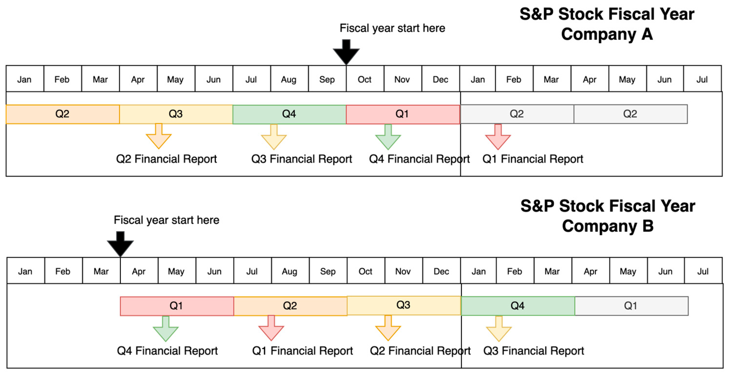
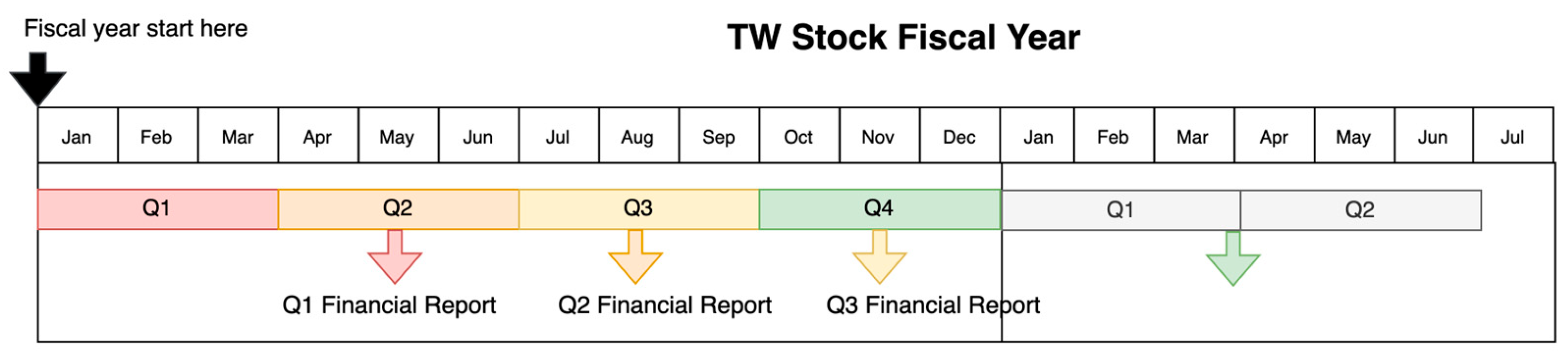
• Aligning data time periods enhances return prediction accuracy and can be applied to other stock markets with fixed fiscal years.
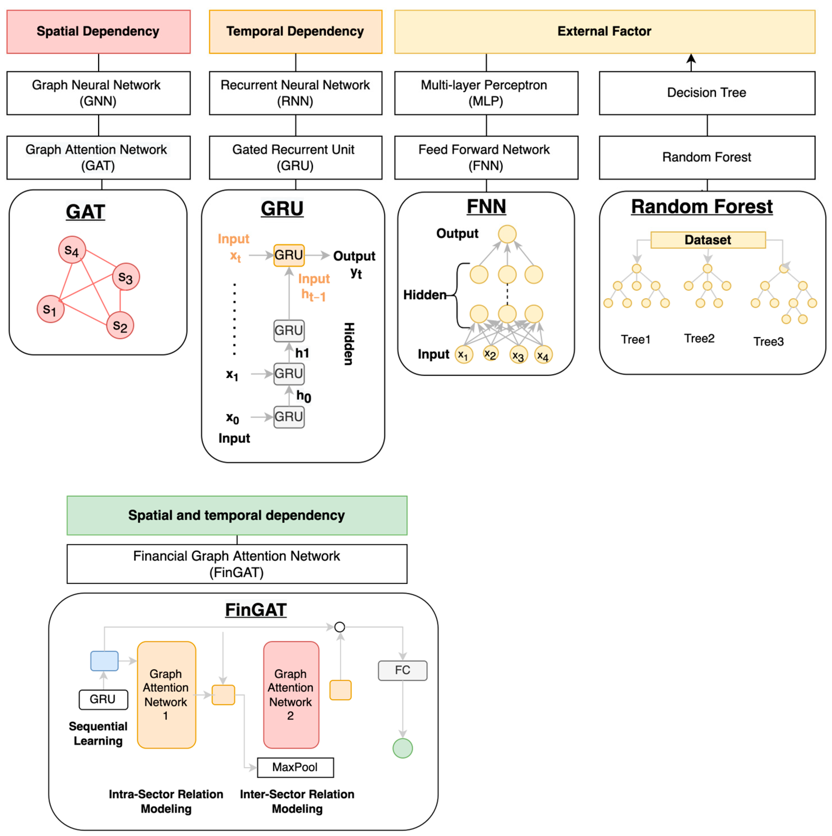
• Four different types of nonlinear models were tested, each with its own strengths and limitations in handling temporal and spatial data dependencies.
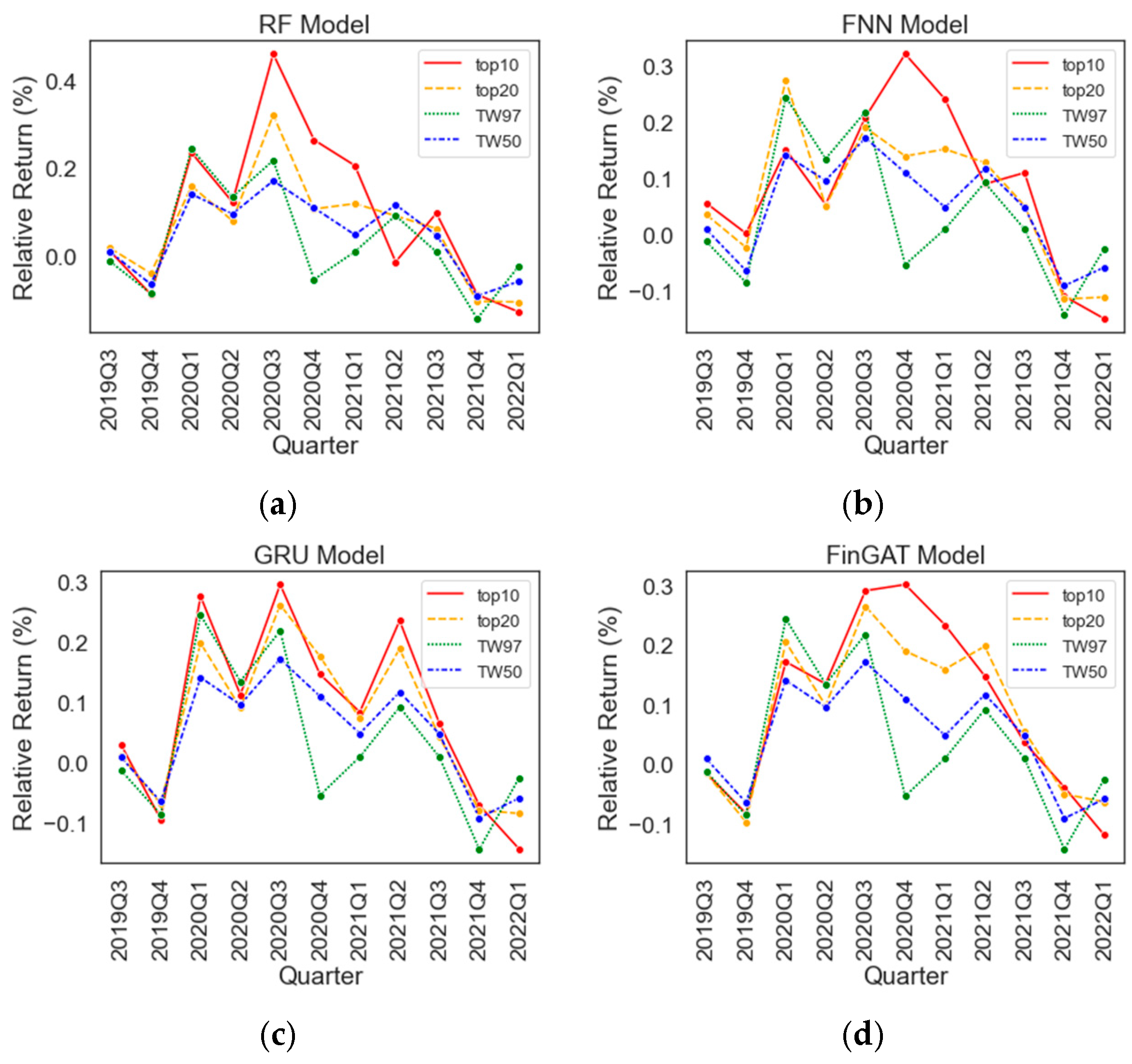
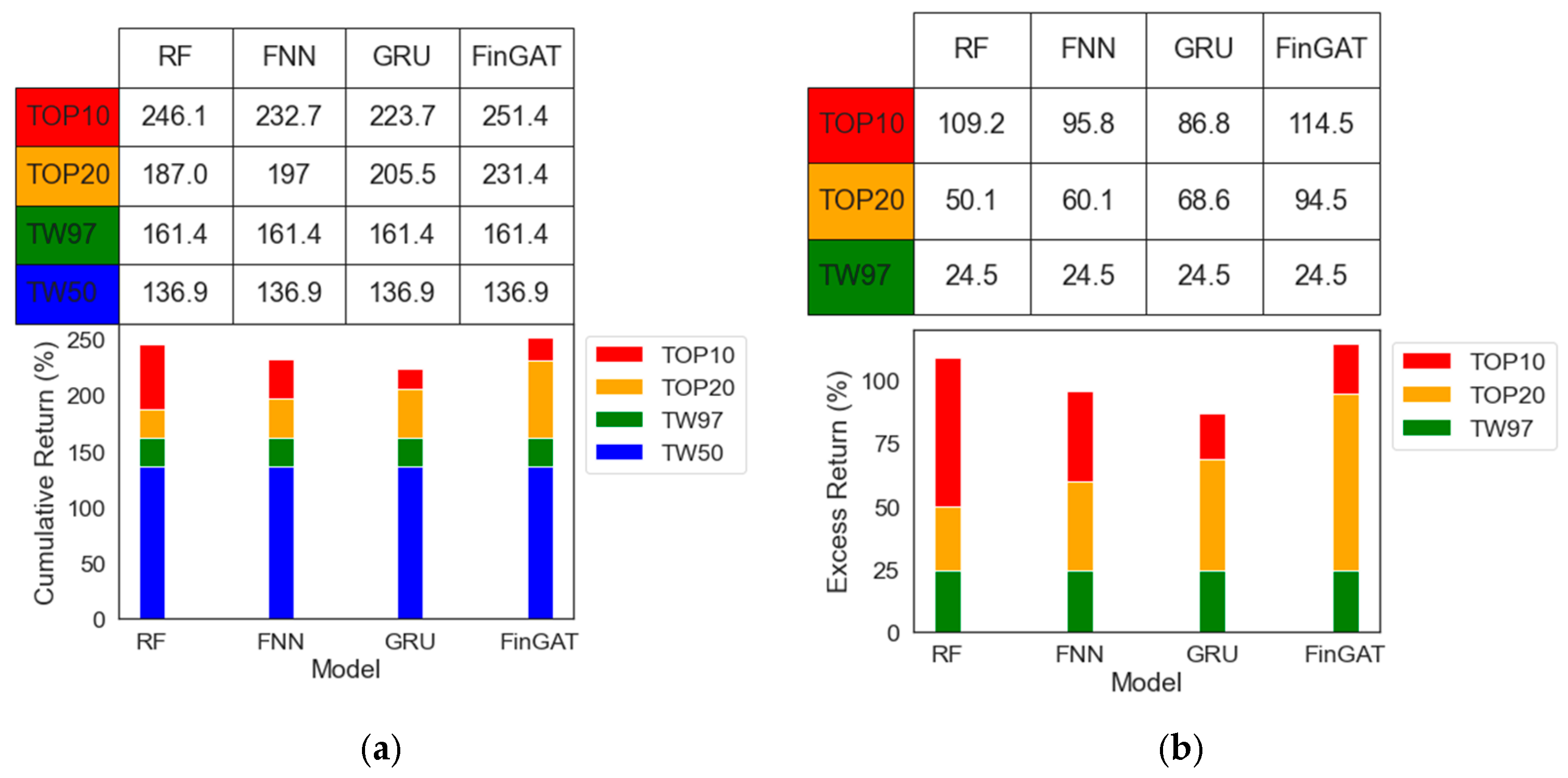
• The top 10 and top 20 stock portfolios generated by our models outperformed the TW50 index with substantial excess returns.
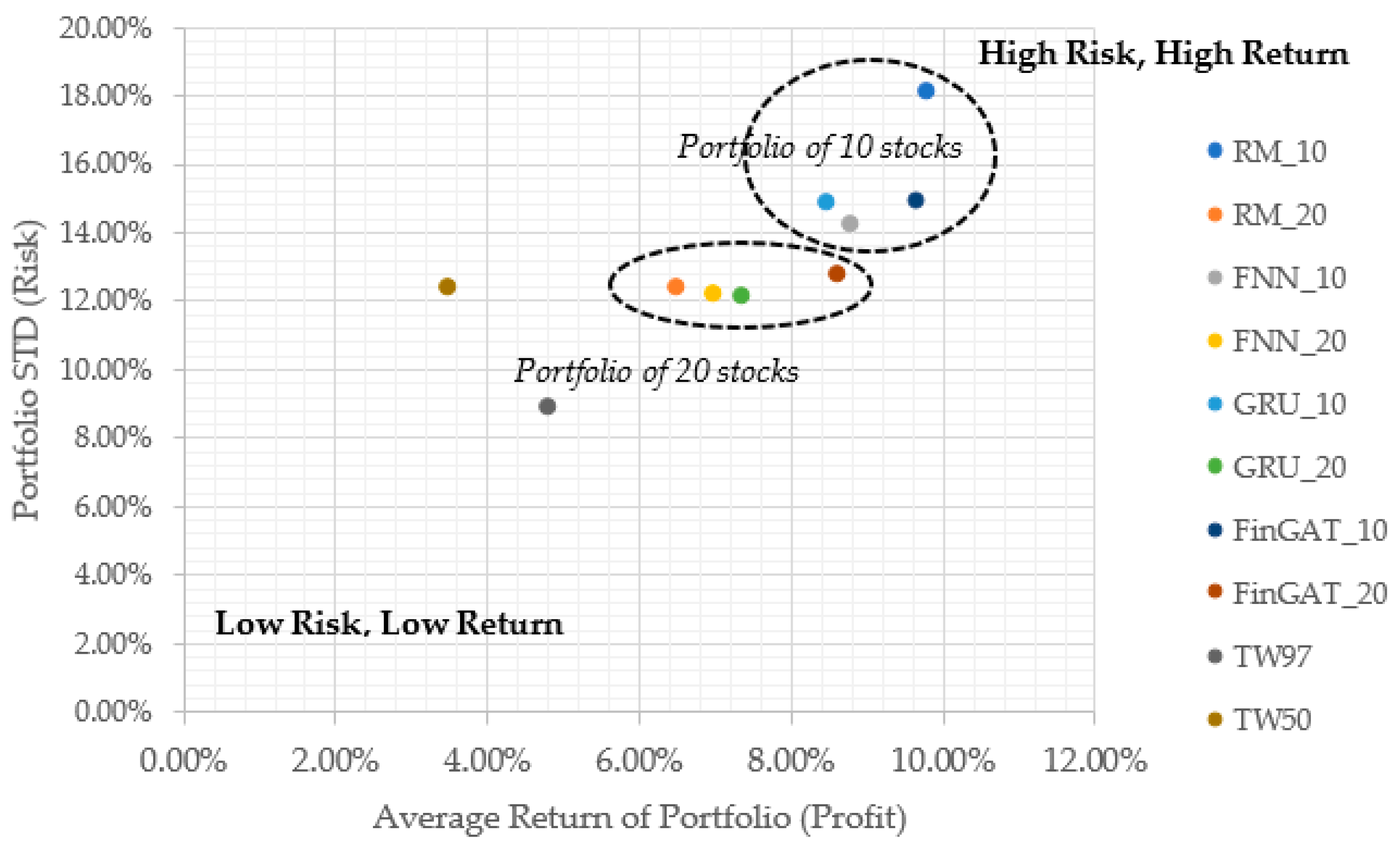
• Our model-selected portfolios also demonstrated lower risk compared to random stock selection or the TW50 index.

In the Taiwanese stock market, investors can now choose 10 or 20 stocks from the stock pool to achieve significant relative returns with acceptable risk, thanks to our model-generated portfolios, in contrast to random stock selection or relying on the TW50 index, which uses a company’s capitalization size as an index.

This paper is organized as follows. We first review the relevant literature in Section 2, followed by presenting the relevant methodologies as in Section 3. Section 4 describes our methodology details. We report the experimental results in Section 5, conclusions in Section 6, and future work in Section 7.

2. Literature Review

In recent years, numerous studies have explored the application of machine learning techniques in stock prediction. H. Yu et al. [10] introduced SVM and PCA in 2014, while X. D. Zhang et al. [11] experimented with AdaBoost in 2016. Additionally, K. Sabbar et al. [12] ventured into stock prediction in 2023, incorporating machine learning and deep learning models. Notably, V. Dhingra et al. [13] in 2021 and K. Olorunnimbe et al. [14] in 2023 delved into deep learning models for this purpose. Most of these studies center on technical and sentiment analysis.

Beyond predictive modeling, there have been surveys and reviews in recent years. I. Ibidapo et al. [15] conducted a study in 2017, and R. M. Dhokane et al. [16] carried out a review in 2023.

In a historical context, the works of B. Graham [17] in 1962 profoundly influenced stock selection and investment. These works span diverse topics, encompassing value investing, fundamental analysis, behavioral finance, risk management, and various investment philosophies rooted in Graham’s enduring principles.

In 1999, Quah and Srinivasan [18] developed a model employing a Feedforward Neural Network (FNN) for stock selection based on quarterly fundamental financial factors. The model demonstrated remarkable success in outperforming the market during testing.

In 2003, Eakins and Stansell [19] employed neural networks to predict stock prices using financial ratios and yearly financial data from 1975 to 1996. Their portfolio of the predicted top 50 stocks outperformed the S&P 500 and Dow Jones Industrial Average.

In 2008, T.S. Quah [20] focused on applying neural networks to fundamental analysis for stock selection in the Dow Jones Industrial Average (DJIA). This research aimed to enhance decision-making processes, offering valuable insights for portfolio management.

In 2018, Namdari and Li [1] utilized an FNN for fundamental analysis to predict stock trends by analyzing 12 financial ratios. Their dataset included 578 companies listed on Nasdaq between June 2012 and February 2017. The FNN model employing fundamental analysis outperformed the one using historical prices.

In 2021, Z.Y. Lu and S.M. Yuan [3] employed an FNN model with 18 financial ratios and sector dummy variables to predict potential stock returns for the next quarter. This approach improved prediction accuracy by incorporating sectors as dummy variables.

In the same year, Huang Y., Capretz L.F., and Ho D. [2] used FNN, Random Forest (RF), and the Adaptive Neural Fuzzy Inference System (ANFIS) to predict potential stock returns by analyzing 20 financial statements and returns. Their portfolio selections yielded substantial excess returns.

W. Chen [21] et al. proposed a novel model, the Graph Convolutional Feature-based Convolutional Neural Network (GC-CNN), for stock prediction in 2021. This model incorporates both individual stock information and stock market data, demonstrating superior performance and adaptability for long-term stock trend prediction.

In 2021, D. Zhang et al. [22] explored the backpropagation algorithm in neural networks for stock price pattern classification and prediction, offering valuable insights for investors and traders.

In 2022, J. Hong et al. [23] introduced a correlational strategy focusing on the analysis of stock technical indicators (STI) and stock movement using neural networks and other machine learning tools. This approach aims to improve prediction accuracy and reduce error rates in stock market analysis, catering to various stockholders’ investment decisions.

3. Preliminaries

In [2], the RF and FNN have better portfolio scores. The GRU and FinGAT models can capture temporal and spatial dependency. Therefore, we chose these four models for our study.

3.1. Random Forest (RF)

Random Forest (RF) stands out as an ensemble learning technique purposefully tailored for stock selection. It draws its inspiration from the concept of decision trees and, during the training process, constructs a multitude of trees. Initially developed by Leo Breiman [5] and Adele Cutler [6], this algorithm is engineered to forge a predictive model for a target variable’s value by assimilating straightforward decision rules from the dataset’s features.

In the realm of stock selection, Random Forest employs a strategic approach. It leverages a random subset of training data and input characteristics to craft each tree within the set. This approach serves the dual purpose of mitigating overfitting concerns and bolstering the model’s capacity to generalize effectively when confronted with unseen data. By incorporating the practice of bootstrap aggregation (bagging), the algorithm further augments tree diversity and curtails variance.

The paramount aim of employing Random Forest for stock selection revolves around forecasting stock performance and behavior, guided by a mosaic of characteristics and factors. Via an examination of historical data and patterns, this model can furnish insights into the potential value or trajectory of stocks, as depicted in Figure 3. Such insights are of paramount importance to investors and traders as they navigate the terrain of making well-informed decisions.

3.2. Feedforward Neural Network (FNN)

The Feedforward Neural Network (FNN) [7,19,24,25,26,27,28,29] emerges as a robust artificial neural network model with notable relevance in the domain of stock selection. Typically, it consists of three or more layers, encompassing an input layer, at least one hidden layer, and an output layer. As depicted in Figure 3, each neuron within a layer establishes connections with every neuron in the subsequent layer.

In the context of stock selection, FNNs are harnessed to model and dissect intricate non-linear relationships between input variables and desired outcomes, such as forecasting stock returns or identifying potential investment prospects. The FNN’s prowess in grasping complex data patterns and dependencies positions it as a highly suitable tool for this endeavor.

The inception of FNN can be traced back to 1990 when Kimoto et al. [24] published its use for forecasting buying and selling signals for the TOPIX index, spanning from January 1987 to September 1989.

In summary, the FNN plays an invaluable role in stock selection by adeptly modeling and scrutinizing non-linear associations between inputs and outputs. Leveraging the backpropagation algorithm, the FNN can be trained to enhance its performance and elevate the precision of stock predictions and investment decisions.

3.3. Gate Recurrent Unit (GRU)

The Gated Recurrent Unit (GRU) is a recurrent neural network (RNN) architecture introduced by Kyunghyun Cho et al. [8] in 2014. It exhibits similarities with the long-short-term memory (LSTM) [26] network and delivers comparable performance. Nevertheless, GRU stands out for its efficiency, as it necessitates fewer parameters, resulting in computational savings compared to LSTM. You can observe the architecture of GRU in Figure 3.

GRU is expressly tailored to handle sequential data, enabling the smooth flow of information from one step to the next. In 2018, M.A. Hossain et al. [30] successfully demonstrated its efficiency in capturing temporal dependencies in sequential data, making it a promising tool for stock selection. Notably, when tested with S&P500 data, it exhibited superior capability in managing the stochastic nature of stock price movements, thus minimizing errors.

In summary, GRU, with its adept handling of sequential data, proves highly effective in analyzing historical stock data and uncovering influential patterns and trends that can impact future stock performance. As a result, GRU assumes a pivotal role in stock prediction models, contributing to the precision of stock selection for investment purposes.

3.4. Graph Attention Network (GAT)

An escalating body of research is delving into the application of graph neural networks (GNNs) within the financial realm, driven by their aptitude for capturing the intricate interconnections between stocks. A study published in 2021 [29] synthesized the typical architectures of GNNs deployed in the financial sector.

The Graph Attention Network (GAT) [31] is a specific subtype of graph neural network (GNN) renowned for its proficiency in dissecting the intricate relationships prevalent in stock markets. The financial domain has witnessed a growing number of investigations delving into the utilization of graph neural networks (GNNs) due to their adeptness at comprehending the intricate linkages between stocks. This research has neatly outlined the prevailing structural patterns of GNNs as applied in finance.

3.5. Financial Graph Attention Network (FinGAT)

In 2021, Hsu, Y. L. et al. [9] introduced an innovative network named FinGAT, which amalgamates the capabilities of the Gated Recurrent Unit (GRU) and the Graph Attention Network (GAT) to forecast stock returns using price data. This method ranked stocks based on their predicted returns and constructed portfolios accordingly. The dataset encompassed 100 stocks in the Taiwan stock market, 424 in the S&P500 index, and 1026 in the NASDAQ index. Impressively, FinGAT outperformed other competing models, including FNN, GRU, and RankLSTM.

FinGAT stands as an advanced neural network meticulously designed for the precise prediction of stock returns. It effectively harnesses the power of graph attention mechanisms to grasp the intricate relationships between diverse stocks. The system comprises three pivotal components: the Gated Recurrent Unit (GRU) for sequential learning, the intra-sector relationship within the Graph Attention Network (GAT), and the inter-sector relationship of GAT, as visualized in Figure 3. The synergy of GAT and GRU is the defining attribute of FinGAT, enabling it to efficiently comprehend and leverage the relationships both within and among sectors of stocks.

Figure 3. Deep learning models including spatial dependency: GNN [32] and GAT [31]; temporal dependency: RNN [33] and GRU [26]; external factor: MLP, FNN [7], and Random Forest [5,6]; and spatial and temporal dependency: FinGAT [9].

Figure 3. Deep learning models including spatial dependency: GNN [32] and GAT [31]; temporal dependency: RNN [33] and GRU [26]; external factor: MLP, FNN [7], and Random Forest [5,6]; and spatial and temporal dependency: FinGAT [9].

4. Methodology

4.1. Stock Pool of TW 97 Stocks

In the context of the Taiwan stock market, our stock pool consists of a fixed set of 97 stocks. These selections were made based on their capitalization rankings on the Taiwan Stock Exchange as of March 2022 and are immutable once established. To benchmark our analysis, we utilize the TW50 [34] index, a stock market index comprising the top 50 companies listed on the Taiwan Stock Exchange, arranged according to market capitalization. These 50 entities collectively represent approximately 70% of the entire market capitalization of the Taiwanese equity market.

We curated these 97 stocks within the stock pools, spanning from 2013Q1 to 2020Q2, encompassing a total of 27 quarters’ worth of financial data. We employed this comprehensive dataset to construct four distinct models aimed at predicting relative returns. Our objective is to identify the top 10 and top 20 stocks which will form our investment portfolio. As a point of reference, the return rate baseline is the portfolio tracked by the TW50 index, which comprises the top 50 companies sorted by market capitalization.

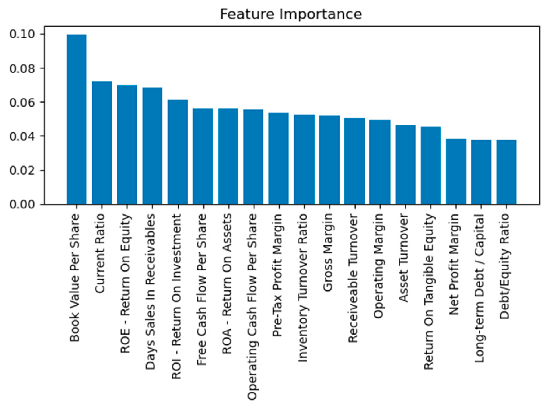
4.2. Financial Ratios of 18 Ratios as Attributes

We use 18 financial ratios as input for models, which are the same as those used in research [3]. The 18 financial ratios are listed, and the calculation formula is given in

Table 1. Financial ratios used for the training model.

Type	Ratio	Calculation
Liquidity Ratios	Current	$\frac{\mathrm{Current}\mathrm{assets}}{\mathrm{Current}\mathrm{liabilities}}$
Leverage Ratios	Debt to Equality	$\frac{\mathrm{Long}\mathrm{Term}\mathrm{Debt}}{\mathrm{Shareholders}’\mathrm{Equality}}$
	Debt to Capital	$\frac{\mathrm{Long}\mathrm{Term}\mathrm{Debt}}{\mathrm{Shareholders}’\mathrm{Equality}+\mathrm{Long}\mathrm{Term}\mathrm{Debt}}$
Asset Efficiency Ratios	Asset Turnover	$\frac{\mathrm{Sales}}{\mathrm{Total}\mathrm{Assets}}$
	Inventory Turnover	$\frac{\mathrm{Sales}}{\mathrm{Inventories}}$
	Receivable Turnover	$\frac{\mathrm{Net}\mathrm{Credit}\mathrm{Sales}}{\mathrm{Receivables}}$
	Days Sales in Receivable	$\frac{\mathrm{Receivables}}{\mathrm{Net}\mathrm{Credit}\mathrm{Sales}}\times 365$
Market Value Ratios	Book Value per Share	$\frac{\mathrm{Shareholders}’\mathrm{Equality}}{\mathrm{Shares}\mathrm{Outstanding}}$
Probability Ratios	Gross Margin	$\frac{\mathrm{Sales}-\mathrm{Cost}\mathrm{of}\mathrm{Goods}\mathrm{Sold}}{\mathrm{Investment}\mathrm{Base}}$
	Operating Margin	$\frac{\mathrm{Operating}\mathrm{Income}\mathrm{Before}\mathrm{Interest}\mathrm{and}\mathrm{Taxes}}{\mathrm{Revenue}}$
	Pre-tax profit margin	$\frac{\mathrm{Sales}-\mathrm{Cost}\mathrm{of}\mathrm{Goods}\mathrm{Sold}}{\mathrm{Investment}\mathrm{Base}}$
	Net Profit Margin	$\frac{\mathrm{Net}\mathrm{Operating}\mathrm{Income}}{\mathrm{Revenue}}$
	Return on Equality	$\frac{\mathrm{Net}\mathrm{Operating}\mathrm{Income}}{\mathrm{Shareholder}’\mathrm{s}\mathrm{Equality}}$
	Return on Tangible Equality	$\frac{\mathrm{Net}\mathrm{Operating}\mathrm{Income}}{\mathrm{Tangible}\mathrm{Shareholder}’\mathrm{s}\mathrm{Equality}}$
	Return on assets	$\frac{\mathrm{Net}\mathrm{Operating}\mathrm{Income}}{\mathrm{Total}\mathrm{Assets}}$
	Return on investment	$\frac{\mathrm{Investment}\mathrm{Gain}}{\mathrm{Investment}\mathrm{Base}}$
	Operating Cash Flow Per Share	$\frac{\mathrm{Operating}\mathrm{Cash}\mathrm{Flow}}{\mathrm{Shares}\mathrm{Outstanding}}$
	Free Cash Flow per Share	$\frac{\mathrm{Operating}\mathrm{Cash}\mathrm{Flow}-\mathrm{Capital}\mathrm{Expenditures}}{\mathrm{Shares}\mathrm{Outstanding}}$

.

There are five main types of financial ratios [4,35]:

• Liquidity ratios: Liquidity ratios measure a company’s ability to pay off its short-term debts.
• Leverage ratios: Leverage ratios measure the amount of debt a company has relative to its assets or equity. These ratios are often used by investors and creditors to assess the riskiness of a company’s operations and its ability to meet long-term debt obligations.
• Asset efficiency ratios: Asset efficiency ratios measure how effectively a company uses and manages its assets to generate revenue.
• Market value ratios: Market value ratios are used to evaluate a company’s stock price in relation to its earnings, sales, and book value.
• Profitability ratios: Profitability ratios measure a company’s ability to generate profits.

4.3. Moving Time Period

In

Table 2. Data split for RF and FNN training, including the moving time period.

RF/FNN	Training Set (20 Quarters)	Validation Set (6 Quarters)	Test Set (1 Quarter)	Moving Time Period During Training and Validation
Moving time period 1	2013Q1–2017Q4	2018Q1–2019Q2	2019Q3	Iterative training 1 Quarter as training input for each moving time period;
Moving time period 2	2013Q2–2018Q1	2018Q2–2019Q3	2019Q4
Moving time period 3	2013Q3–2018Q2	2018 Q3–2019 Q4	2020Q1
……	……	……	……
Moving time period 11	2015Q3–2020Q2	2020Q3–2021Q4	2022Q1

, the RF and FNN models encompass a total of 27 quarters for each moving time period. The initial data from the moving time period span from 2013Q1 to 2019Q4, and so forth. We partitioned these data into three segments: the training set, the validation set, and the test set, comprising 20 quarters, 6 quarters, and 1 quarter, respectively. The training set facilitates model weight optimization, and the validation set aids in fine-tuning hyperparameters, ensuring model convergence without overfitting. Subsequently, we employ the test set to predict the relative return of the 97 stocks within the pool. A comprehensive analysis of the model prediction results is presented in Section 4.

In

Table 3. Data split for GRU and FinGAT training, including the moving time period.

GRU/FinGAT	Training Set (20 Quarters)	Validation Set (6 Quarters)	Test Set (4 Quarter)	Moving Time Period During Training and Validation
Moving time period 1	2013Q1–2017Q4	2018Q1–2019Q2	2019Q3–2020Q2	Iterative training 4 Quarters as training input for each moving time period;
Moving time period 2	2013Q2–2018Q1	2018Q2–2019Q3	2019Q4–2020Q3
Moving time period 3	2013Q3–2018Q2	2018 Q3–2019 Q4	2020Q1–2020Q4
……	……	……	……
Moving time period 11	2015Q3–2020Q2	2020Q3–2021Q4	2022Q1–2022Q4

, the GRU and FinGAT models span a total of 30 quarters for each moving time period, with the initial data originating from 2013Q1 to 2020Q2 and so on. We segment this data into the training set, validation set, and test set, consisting of 20 quarters, 6 quarters, and 4 quarters, respectively. Similar to the previous models, the training set facilitates model weight optimization, and the validation set aids in hyperparameter fine-tuning, guaranteeing model convergence without overfitting. The test set is then leveraged to predict relative returns across a total of 11 models. A detailed evaluation of the model prediction results is expounded upon in Section 4.

Via these distinct moving time periods, we established 11 trained models, each attuned to specific temporal data segments. This approach enables us to effectively glean insights into the stock trends within our stock pool. It serves as the foundation for our training and testing datasets for RF, FNN, GRU, and FinGAT, empowering comprehensive analysis and evaluation.

4.4. Evaluation Metrics

To assess the performance of portfolios assembled with each model, we employ four key metrics: excess return, top-k precision, and portfolio score. These metrics collectively address both the return profitability and risk associated with the portfolios.

4.4.1. Excess Return

Excess returns are a useful measure to evaluate the performance of an investment portfolio. By comparing portfolio returns to those of a benchmark, investors can determine whether the portfolio is generating value above the benchmark.

The excess return on a benchmark (ER_benchmark) of portfolio p for quarter q is formulated as follows in Equation (1):

$${\mathrm{ER}}_{\mathrm{p}}=\left\{{\prod }_{\mathrm{q}=1}^{\#\mathrm{quarters}}1+{\mathrm{R}}_{\mathrm{p}}\left(\mathrm{q}\right)\right\}-\left\{{\prod }_{\mathrm{q}=1}^{\#\mathrm{quarters}}1+{\mathrm{R}}_{\mathrm{benchmark}}\left(\mathrm{q}\right)\right\}$$

(1)

where ${\mathrm{R}}_{\mathrm{p}}\left(\mathrm{q}\right)$ is the actual absolute return, and ${\mathrm{R}}_{\mathrm{TW}50}\left(\mathrm{q}\right)$ is the actual absolute return of our TW stock benchmark of the TW50 index.

4.4.2. Top-k Precision

The precision of k is used to measure the percentage of overlap between a list of top k stocks with the highest predicted returns, which is ‘predicted top k stocks’, and a list of top k stocks with the highest actual return, which is ‘actual top k stocks’. The higher the precision of the top-k, the more accurate the prediction of the model will be.

Top-k precision can be calculated as follows via Equation (2):

$$\mathrm{Top}-\mathrm{k}\mathrm{precision}=\frac{|\mathrm{L}@\mathrm{K}({\mathrm{R}}_{\mathrm{q}}^{\mathrm{S}})\cap \mathrm{L}@\mathrm{K}({\widehat{\mathrm{R}}}_{\mathrm{q}}^{\mathrm{S}}\left)\right|}{\mathrm{K}}$$

(2)

$\mathrm{L}@\mathrm{K}\left({\mathrm{R}}_{\mathrm{q}}^{\mathrm{S}}\right)$ is the expected top-k precision of a portfolio consisting of randomly selected k stocks as Equation (3). In that case, top-k precision can be served as follows:

$$\mathrm{Top}-\mathrm{k}\mathrm{precision}=\frac{\mathrm{K}}{\#\mathrm{stocks}\mathrm{in}\mathrm{stock}\mathrm{pool}}$$

(3)

The benchmarks for the precision of top-10 and top-20 in the Taiwan stock market are 10.3% (calculated as 10/97) and 20.6% (calculated as 20/97), respectively.

4.4.3. Portfolio Score

When assessing a portfolio’s performance, it is crucial to account for not only the return’s profitability but also the inherent risk associated with the investment. Both elements collectively paint a more comprehensive picture of the portfolio’s performance. For instance, even if a portfolio exhibits the potential for high returns if its performance is marked by significant volatility from one quarter to the next, it may not be an attractive choice for investors.

In our study, we use the same modified portfolio score [2] to measure the equally weighted portfolio p as used in previous research. In Equation (4), a higher portfolio score indicates the selection of a portfolio with high return and low risk.

$$\mathrm{Portfolio}\mathrm{Score}=\frac{{\overline{\mathrm{R}}}_{\mathrm{p}}}{{\mathsf{\sigma }}_{\mathrm{p}}}$$

(4)

${\overline{\mathrm{R}}}_{\mathrm{p}}$ in Equation (5) is the average actual relative return that had subtracted with the TW50 index quarterly, as given below:

$${\overline{\mathrm{R}}}_{\mathrm{p}}=\frac{1}{\#\mathrm{quarters}}{\sum }_{\mathrm{q}=1}^{\#\mathrm{quarters}}{\mathrm{R}}_{\mathrm{p}}\left(\mathrm{q}\right)$$

(5)

${\mathrm{R}}_{\mathrm{p}}\left(\mathrm{q}\right)$ is the actual absolute return for quarter q.

4.5. Model Architecture for Training/Validation/Test

4.5.1. Data Clean

After data collection, the following steps are ‘data standardization’ to ensure the mean of the characteristic is at 0 and the standard deviation is at 1 for all features. Data standardization can help create a more consistent and reliable dataset. Moreover, it can help the algorithm to search the effective path for relative global minimum and not be easily trapped by local minimum during model training. We use the z score to standardize the vector of features x with the following formula:

$$\mathrm{z}=\frac{\mathrm{x}-\mathsf{\mu }}{\mathsf{\sigma }}$$

where μ is the mean of x, and σ is the standard deviation of x.

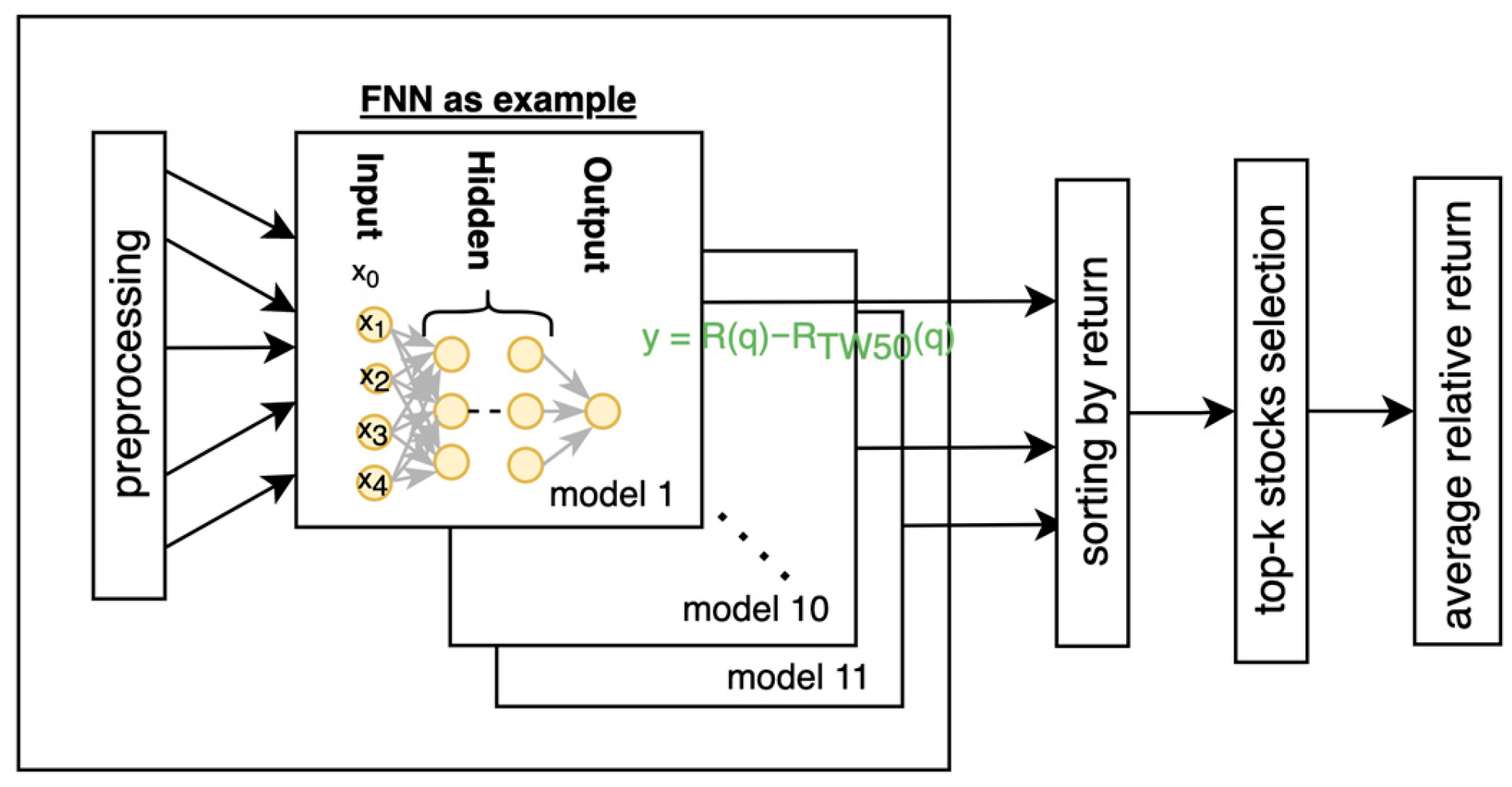
4.5.2. Relative Return as Target y in Training

The absolute returns quarterly of stock is defined as follows in Equation (6):

$$\frac{\mathrm{price}({\mathrm{q}}_{\mathrm{end}})}{\mathrm{price}({\mathrm{q}}_{\mathrm{start}})}-1$$

(6)

The price (${\mathrm{q}}_{\mathrm{end}})$ is the stock’s price on the last day of quarter q, and the (${\mathrm{q}}_{\mathrm{start}})$ is the stock’s price on the first day of quarter q.

The optimization variable y is the relative quarterly return of a stock as in Equation (7):

$$\mathrm{R}\left(\mathrm{q}\right)-{\mathrm{R}}_{\mathrm{TW}50}\left(\mathrm{q}\right)$$

(7)

R(q) is the quarterly absolute return of stock for quarter q, and the R_TW50(q) is the quarterly return of the TW50 index as a benchmark portfolio.

The absolute return of a stock is susceptible to influence not just from the company’s performance but also from the broader stock market conditions. This inherent volatility makes it a less stable target for model learning. Consequently, we perform preprocessing by converting absolute returns into relative returns, which serves as the training target for our modeling efforts.

4.5.3. Training Procedure

The training set, validation set, and test set are constructed by progressing via different time periods, as elucidated in Section 3.3.

Once a model has been meticulously trained and fine-tuned, the test data are fed into the respective moving time period model. This process yields predicted returns for all 97 stocks within the portfolio. Subsequently, the returns are sorted in descending order for each moving time period. Following this sorting, the top 10 stocks with the highest returns and the top 20 stocks with the highest returns are chosen to constitute the top 10 and top 20 portfolios across all moving time periods, as depicted in Figure 4.

For each model, we use the scikit-learn library in Python to develop models. And we list the hyperparameters of each model in Section 3.1, Section 3.2, Section 3.3, Section 3.4 and Section 3.5, including RF, FNN, GRU, and FinGAT.

4.5.4. Random Forest Hyperparameters

We use Pytorch to develop the FNN models. Hyperparameters of random forest are tuned with the validation set for preventing overfitting where the number of estimators is 1000 and the optimization criterion used squared_error.

The test result shows that the random forest model for generating top-10 as a portfolio with a 109.2% relative return of 109.2% to the TW50 index and top-20 as a portfolio with a 50.1% relative return of 50.1% to the TW50 index. The 97 composite index achieves only a 24.5% relative return of 24.5% to the TW50 index.

In Figure 5, the importance of the random forest characteristics shows that all 16 financial indices are similar in importance with no redundant features.

4.5.5. FNN Hyperparameters

We use Pytorch to develop FNN models. Hyperparameters of FNN are tuned using the validation set to prevent overfitting, as shown in

Table 4. Hyperparameters of FNN models.

Name of Hyperparamter	Optimized Result
Number of hidden layers	2
Number of nodes in the first hidden layer	30
Number of nodes in the second hidden layer	15
Loss Function	MSE
Activation Function	Sigmoid
Learning Rate	1 × 10−3
Optimizer	Adam
Learning Rate Scheduler	ReduceLROnPlateau with factor = 0.1

.

4.5.6. GRU Architecture

We use Pytorch to develop GRU models. Hyperparameters of GRU are tuned using the validation set to prevent overfitting, as shown in

Table 5. Hyperparameters of GRU models.

Name of Hyperparamter	Optimized Result
Number of hidden layers	1
Dimension of hidden state	36
Time Step (Ratios of four quarters are inputted to GRU)	4
Activation Function	Sigmoid
Loss Function	MSE
Number of training epochs	100
Learning Rate	1 × 10−3
Optimizer	Adam
Learning Rate Scheduler	ReduceLROnPlateau with factor = 0.1

.

4.5.7. FinGAT Hyperparameter

We use Pytorch to develop FinGAT models. Hyperparameters of FinGAT are tuned using the validation set to prevent overfitting, as shown in

Table 6. Hyperparameters of FinGAT models.

Name of Hyperparamter	Optimized Result
Number of layers in GRU	1
Number of layers in GAT	1
Dimension of Hidden State of GRU and GAT	20
GRU time step (Ratios of four quarters are inputted to GRU)	3
Activation Function	Sigmoid
Loss Function	MSE
Number of training epochs	100
Learning Rate	1 × 10−3
Optimizer	Adam
Learning Rate Scheduler	ReduceLROnPlateau with factor = 0.1

.

There are a total of 11 sectors of TW stocks, and the distribution for the 97 stocks in the pool is shown in

Table 7. Sector distribution of 97 TW stocks in the pool.

Sector	Total Number of Shares in 97 Stocks of TW
Basic Material	10
Communication Service	3
Consumer Cyclical	9
Consumer Defensive	3
Energy	1
Financial Services	15
Healthcare	0
Industrials	11
Real Estate	1
Technology	44
Utility	0
Total	97

.

5. Results

We plot the relative return of four models in Figure 6 by quarter. Each trained model is used to select the highest 10 and highest 20 stocks for the top-10 and top-20 relative returns in red and orange, respectively. The TW 97 used all stocks in the pool to investigate and calculate the relative return in the green line. Then, the TW50 index is the portfolio as the benchmark for stock selection in the blue line.

The area under the relative return curve shows how the portfolio performs during that investigation period. While using the TW50 index as the benchmark, the larger area between each portfolio and the TW50 blue line shows that the portfolio obtains better returns.

Overall, the selected top 10 and top 20 portfolios by trained models perform better than the TW50 index portfolio.

We calculated the indexes, including portfolio score, excess return, average return of a portfolio, top-k precision, and STD of portfolio for comparison of different portfolio models in

Table 8. Portfolio score, excess return, average return of a portfolio, top-k precision, and STD of portfolio. These indexes are used to compare different portfolio models.

	Random Forest		FNN		GRU		FinGAT		TW 97	TW 50
Portfolios	Top 10	Top 20	Top 10	Top 20	Top 10	Top 20	Top 10	Top 20
Portfolio Score	0.54	0.53	0.62 (3)	0.58	0.58	0.61	0.65 (2)	0.68 (1)	0.54	0.29
Excess return to the TW50 index	109.2% (2)	50.1%	95.8% (3)	60.1%	65%	79%	114.5% (1)	94.5%	23.5%	Baseline 0%
Average Return of Portfolio	9.8% (1)	6.5%	8.8% (3)	7.0%	8.5%	7.39%	9.67% (2)	8.61%	4.8%	3.5%
Top-k Precision	16.4% 1	26.8% 2 (3)	19.1% 1	27.7% 2 (1)	18.2% 1	29.5% 2	21.8% 1	27.3% 2 (2)	NA	NA
STD of portfolio	18.1%	12.3%	14.2%	12.2%	14.8%	12.12%	14.87%	12.67%	8.9%	12.3%

¹ The benchmark for top 10 precision in the stock pool is 10.3% (calculated as 10/97). ² The benchmark for top 20 in the stock pool is 20.6% (calculated as 20/97).

. The results were discussed in the following subsections.

5.1. High Portfolio Scores

The portfolio score, as detailed in Section 3.3 and expressed in Equation (5), serves as a metric designed to strike an equilibrium between stock return profitability and investment risk. It is calculated by averaging the returns over quarters and dividing by the investment risk. Higher portfolio scores denote a stable and advantageous portfolio from a financial perspective.

The FinGAT model showcases the most impressive excess return among all portfolios. This outcome can be attributed to the amalgamation of temporal and spatial models within the FinGAT framework for predicting stock returns. Notably, the sector-specific information demonstrates that FinGAT’s top 20 portfolios not only yield substantial excess returns but also reduce risk compared to RM of Top-20.

The portfolio score in TW stock with aligned fiscal year data shows improvement in stock prediction compared with the portfolio score of RF in S&P stock as in

Table 9. Portfolio score of Top-20 with RF and FNN models in US S&P stock market and TW stock market.

Top-20	Research of US S&P [2]	Ours of TW Stock
	Portfolio Score	Portfolio Score
RF	0.414	0.58
FNN	0.202	0.53

with RF and FNN models of 0.166 and 0.328 [2], respectively. This proves our hypothesis that not only modeling will affect the stock price prediction but also fiscal year alignment, which is a key factor in stock price prediction.

5.2. High Excess Return in Top-10 and Top-20 in Test Data for Four Models for Investment Gain

The excess return for the top 10, top 20, and TW97 portfolios, as well as the TW50 index during the period from 2019Q3 to 2022Q1, spanning a total of 11 quarters, is presented in Figure 7a. Notably, all portfolio types, including the top-10, top-20, TW97, and the TW50 index, exhibit excess returns exceeding 135%.

When we consider the relative excess return compared to the TW50 index, as displayed in Figure 7b, the RF and FinGAT models achieve 109.2% and 114% for op-10 portfolios, respectively. It is worth noting that the top-10 portfolio consistently outperforms the top-20 portfolio. Among the four models, RF and FinGAT stand out due to their pronounced nonlinearity in capturing stock trends, making them noteworthy choices for stock trend learning.

5.3. Low-Risk Investment and High Return Rate

In Table 3, the columns representing the average return on investment (investment profit) and the standard deviation of a portfolio (investment risk) serve as critical indicators of the model’s proficiency in managing investment risks. To provide a clearer insight into the relationship between risk and return, we created a scatter plot in Figure 8. The x-axis represents risk, while the y-axis depicts return, encompassing all portfolios and the TW50 index.

As evident in Figure 8, the principle that a higher number of stocks in a portfolio corresponds to increased risk and augmented return holds true, a phenomenon corroborated by the data.

Furthermore, a black regression line is plotted, intersecting with the TW50 index, which serves as our benchmark. The upper right side of this line signifies high risk with substantial portfolio investment, while the lower left side denotes lower risk with more conservative portfolio investment.

Exploring the implications of varying the value of k for portfolios ranging from the top 5 to the top 40 will be a future research endeavor. This study will delve into how the hyperparameter k influences both profit and investment risk within the TW stock market context, offering valuable insights into portfolio optimization.

5.4. Top-k Precision

The top-k precision metric is instrumental in gauging the concordance between the list of chosen top-k stocks, those with the highest predicted returns, and the actual outcomes during that specific quarter. As elaborated in Section 5.2, a higher top-k precision underscores the model’s capacity for accurate return predictions.

For the four models, namely RF, FNN, GRU, and FinGAT, the top-10 portfolio model selections exhibited overlaps with the ground truth (GT) at percentages of 16.4%, 19.1%, 18.2%, and 21.8%, respectively. In contrast, the baseline precision of a random shuffle comprising 10 stocks from the pool of 97 stocks amounted to 10.3%. In summation, our modeling endeavors showcased their potential by enhancing precision, elevating it by approximately 6.4% to 11.8% for top 10 portfolios.

The precision of the top 20 portfolios in the RF, FNN, GRU, and FinGAT models was recorded at 26.8%, 27.7%, 29.5%, and 27.3%, respectively. In contrast, the random shuffle baseline for selecting 20 stocks from the pool of 97 stocks yielded a precision of 20.6%. In conclusion, the utilization of modeling for the selection of 20 stocks in a top 20 portfolio boosted precision by approximately 6.2% to 9.3%.

It is noteworthy that top 20 portfolios exhibit higher precision compared to top 10 portfolios, thereby entailing lower investment risk. However, this comes at the trade-off of relatively lower returns. Investors are encouraged to choose their model based on their income and risk tolerance, ensuring they opt for the most suitable option that aligns with their risk acceptance and financial objectives.

6. Conclusions

The successful utilization of RF, FNN, GRU, and FinGAT models holds significant managerial implications for enhancing portfolio management strategies:

• Improved Stock Selection: The superior performance of our models, particularly in comparison to the TW50 benchmark, positions them as valuable tools for stock selection. This enhances the decision-making process for portfolio managers, providing more effective alternatives for discerning investors.
• Consideration of Fiscal Year Alignment: Managers should be aware of the limitations regarding aligned fiscal years. In markets with misaligned fiscal years, there may be potential performance loss due to quarterly financial report publishing misalignment. This suggests a need for adaptation or additional considerations when applying these models in diverse fiscal environments.
• Optimal Risk–Return Balance: The demonstrated balance between return and risk, as showcased in the risk vs. return plot, highlights the efficiency of our risk and return management approach. This implies that managers can achieve higher returns without significantly increasing portfolio risk, offering a valuable strategy for optimizing risk-adjusted returns.
• Methodological Prowess: The consistently superior performance of our methodology, as evidenced by portfolio scores outperforming the TW50 index, underscores its prowess. This emphasizes the reliability and effectiveness of our approach, reinforcing the commitment to sound risk and return management practices.
• Precision Improvement: Although precision in top 10 and top 20 outcomes may not be significant, the approach significantly outperforms random stock selection. This suggests that managers can enhance accountability by relying on our models, achieving more predictable outcomes in the range of 6.4% to 11.8% for top 10 portfolios and 6.2% to 9.3% for top 20 portfolios.
• Expanded Investment Options: The diversity of choices beyond TW50 index portfolios or haphazard stock selection offers investors a more tailored approach. Managers can guide investors to opt for top 10 portfolios for high excess returns with acceptable risk or top 20 portfolios for lower risk, maintaining commendable excess returns relative to the TW50 index.

In conclusion, these managerial implications emphasize the strategic advantages and adaptability of our models, providing valuable insights for optimizing portfolio performance in dynamic market conditions.

7. Future Work

In conclusion, the Random Forest model stands out as the second-highest performer within the top 10 portfolios. To further enhance its risk–return profile, we may explore the incorporation of additional financial ratios into the Random Forest modeling in the future, aiming to maintain robust returns while mitigating risk.

Moving forward, we plan to refine the value of k as a hyperparameter, which will provide investors with more flexibility. Currently, we adhere to k values of 10 and 20, but fine-tuning this parameter could offer greater options for portfolio customization.

Furthermore, our current approach employs equal weights for stocks within a portfolio. A prospective avenue for improvement involves training weights for individual stocks within the same portfolio. This adjustment aligns more closely with stock market dynamics, in which certain stocks may outperform due to societal or politically relevant topics.

Additionally, we are intrigued by the prospect of applying our methodology to stock markets that share the same fiscal year alignment as the TW stock market, facilitating performance comparisons across different financial markets. This endeavor promises to yield valuable insights into stock selection strategies and investment opportunities.

References

1. Namdari, A.; Li, Z.S. Integrating fundamental and technical analysis of stock market through multi-layer perceptron. In Proceedings of the 2018 IEEE Technology and Engineering Management Conference (TEMSCON), Evanston, IL, USA, 28 June–1 July 2018; pp. 1–6. [Google Scholar]
2. Huang, Y.; Capretz, L.F.; Ho, D. Machine learning for stock prediction based on fundamental analysis. In Proceedings of the 2021 IEEE Symposium Series on Computational Intelligence (SSCI), Orlando, FL, USA, 5–7 December 2021; pp. 1–10. [Google Scholar]
3. Lu, Z.-Y. A Deep Reinforcement Learning-Enabled Portfolio Management System with Quarterly Stock Re-Selection Based on Financial Statements. Master’s Thesis, National Yang Ming Chiao Tung University, Taiwan, China, 2022. [Google Scholar]
4. Arkan, T. The importance of financial ratios in predicting stock price trends: A case study in emerging markets. Finanse Rynki Finansowe Ubezpieczenia 2016, 79, 13–26. [Google Scholar] [CrossRef]
5. Breiman, L. Random forests. Mach. Learn. 2001, 45, 5–32. [Google Scholar] [CrossRef]
6. Cutler, A.; Cutler, D.R.; Stevens, J.R. Random forests. In Ensemble Machine Learning: Methods and Applications; Springer: New York, NY, USA, 2012; pp. 157–175. [Google Scholar]
7. Svozil, D.; Kvasnicka, V.; Pospichal, J. Introduction to multi-layer feed-forward neural networks. Chemom. Intell. Lab. Syst. 1997, 39, 43–62. [Google Scholar] [CrossRef]
8. Cho, K.; Van Merriënboer, B.; Gulcehre, C.; Bahdanau, D.; Bougares, F.; Schwenk, H.; Bengio, Y. Learning phrase representations using RNN encoder-decoder for statistical machine translation. arXiv 2014, arXiv:1406.1078. [Google Scholar]
9. Hsu, Y.-L.; Tsai, Y.-C.; Li, C.-T. FinGAT: Financial Graph Attention Networks for Recommending Top-KK Profitable Stocks. IEEE Trans. Knowl. Data Eng. 2021, 35, 469–481. [Google Scholar] [CrossRef]
10. Yu, H.; Chen, R.; Zhang, G. A SVM stock selection model within PCA. Procedia Comput. Sci. 2014, 31, 406–412. [Google Scholar] [CrossRef]
11. Zhang, X.-d.; Li, A.; Pan, R. Stock trend prediction based on a new status box method and AdaBoost probabilistic support vector machine. Appl. Soft Comput. 2016, 49, 385–398. [Google Scholar] [CrossRef]
12. Sabbar, K.; El Kharrim, M. Average variance portfolio optimization using machine learning-based stock price prediction case of renewable energy investments. In E3S Web of Conferences; EDP Sciences: Ulys, France, 2023; Volume 412, p. 01077. [Google Scholar]
13. Dhingra, V.; Sharma, A.; Gupta, S.K. Sectoral portfolio optimization by judicious selection of financial ratios via PCA. Optim. Eng. 2023, 1–38. [Google Scholar] [CrossRef]
14. Olorunnimbe, K.; Viktor, H. Deep learning in the stock market—A systematic survey of practice, backtesting, and applications. Artif. Intell. Rev. 2023, 56, 2057–2109. [Google Scholar] [CrossRef] [PubMed]
15. Ibidapo, I.; Adebiyi, A.; Okesola, O. Soft computing techniques for stock market prediction: A literature survey. Covenant J. Inform. Commun. Technol. 2017, 5, 1–28. [Google Scholar]
16. Dhokane, R.M.; Sharma, O.P. A Comprehensive Review of Machine Learning for Financial Market Prediction Methods. In Proceedings of the 2023 International Conference on Emerging Smart Computing and Informatics (ESCI), Pune, India, 1–3 March 2023; pp. 1–8. [Google Scholar]
17. Graham, B.; Dodd, D.L.F.; Cottle, S.; Tatham, C. Security Analysis: Principles and Technique; McGraw-Hill: New York, NY, USA, 1962. [Google Scholar]
18. Quah, T.-S.; Srinivasan, B.; Lee, M. Segmental Stock Market Prediction Using Neural Network. In Proceedings of the Applied Informatics-Proceedings, Innsbruck, Austria, 15–18 February 1999; pp. 23–24. [Google Scholar]
19. Eakins, S.G.; Stansell, S.R. Can value-based stock selection criteria yield superior risk-adjusted returns: An application of neural networks. Int. Rev. Financ. Anal. 2003, 12, 83–97. [Google Scholar] [CrossRef]
20. Quah, T.-S. DJIA stock selection assisted by neural network. Expert Syst. Appl. 2008, 35, 50–58. [Google Scholar] [CrossRef]
21. Chen, W.; Jiang, M.; Zhang, W.-G.; Chen, Z. A novel graph convolutional feature based convolutional neural network for stock trend prediction. Inf. Sci. 2021, 556, 67–94. [Google Scholar] [CrossRef]
22. Zhang, D.; Lou, S. The application research of neural network and BP algorithm in stock price pattern classification and prediction. Future Gener. Comput. Syst. 2021, 115, 872–879. [Google Scholar] [CrossRef]
23. Hong, J.; Han, P.; Rasool, A.; Chen, H.; Hong, Z.; Tan, Z.; Lin, F.; Wei, S.X.; Jiang, Q. A Correlational Strategy for the Prediction of High-Dimensional Stock Data by Neural Networks and Technical Indicators. In International Conference on Big Data and Security; Springer: Singapore, 2022; pp. 405–419. [Google Scholar]
24. Kimoto, T.; Asakawa, K.; Yoda, M.; Takeoka, M. Stock market prediction system with modular neural networks. In Proceedings of the 1990 IJCNN International Joint Conference on Neural Networks, San Diego, CA, USA, 17–21 June 1990; pp. 1–6. [Google Scholar]
25. Quah, T.-S. Improving returns on stock investment through neural network selection. In Artificial Neural Networks in Finance and Manufacturing; IGI Global: Hershey, PA, USA, 2006; pp. 152–164. [Google Scholar]
26. Chung, J.; Gulcehre, C.; Cho, K.; Bengio, Y. Empirical evaluation of gated recurrent neural networks on sequence modeling. arXiv 2014, arXiv:1412.3555. [Google Scholar]
27. Matsunaga, D.; Suzumura, T.; Takahashi, T. Exploring graph neural networks for stock market predictions with rolling window analysis. arXiv 2019, arXiv:1909.10660. [Google Scholar]
28. Tsai, Y.-C.; Chen, C.-Y.; Ma, S.-L.; Wang, P.-C.; Chen, Y.-J.; Chang, Y.-C.; Li, C.-T. FineNet: A joint convolutional and recurrent neural network model to forecast and recommend anomalous financial items. In Proceedings of the 13th ACM Conference on Recommender Systems, Copenhagen, Denmark, 16–20 September 2019; pp. 536–537. [Google Scholar]
29. Wang, J.; Zhang, S.; Xiao, Y.; Song, R. A review on graph neural network methods in financial applications. arXiv 2021, arXiv:2111.15367. [Google Scholar] [CrossRef]
30. Hossain, M.A.; Karim, R.; Thulasiram, R.; Bruce, N.D.; Wang, Y. Hybrid deep learning model for stock price prediction. In Proceedings of the 2018 IEEE Symposium Series on Computational Intelligence (SSCI), Bangalore, India, 18–21 November 2018; pp. 1837–1844. [Google Scholar]
31. Veličković, P.; Cucurull, G.; Casanova, A.; Romero, A.; Lio, P.; Bengio, Y. Graph attention networks. arXiv 2017, arXiv:1710.10903. [Google Scholar]
32. Scarselli, F.; Gori, M.; Tsoi, A.C.; Hagenbuchner, M.; Monfardini, G. The graph neural network model. IEEE Trans. Neural Netw. 2008, 20, 61–80. [Google Scholar] [CrossRef] [PubMed]
33. Medsker, L.R.; Jain, L. Recurrent neural networks. Des. Appl. 2001, 5, 2. [Google Scholar]
34. Taiwan Index Plus. Available online: https://taiwanindex.com.tw/en/indexes/TW50 (accessed on 1 July 2023).
35. Ehrhardt, M.C. Financial Management: Theory and Practice; South-Western Cengage Learning: Mason, OH, USA, 2011. [Google Scholar]
Figure 1. In the S&P stock market, some companies, such as Company A, start their fiscal year in September, and others, such as Company B, start their fiscal year in April. The misaligned starting point of the fiscal year makes the publishing of financial reports time misaligned due to different market businesses.
Mathematics 11 04758 g001
Figure 2. In the TW stock market, the fiscal year is aligned to start in January as Q1 for all companies. And the yearly financial report will be public before March the next year.
Mathematics 11 04758 g002
Figure 4. Model training architecture for RF, FNN, GRU, and FinGAT, with FNN as an example in the figure.
Mathematics 11 04758 g004
Figure 5. Importance of features of random forest models.
Mathematics 11 04758 g005
Figure 6. Relative return with different portfolios of (a) RF model, (b) FNN model, (c) GRU model, and (d) FinGAT model.
Mathematics 11 04758 g006
Figure 7. The relative return for 4 models with 4 portfolios from 2019Q3 to 2022Q1, a total of 11 quarters: (a) cumulative return of top 10, top 20, TW97, and TW50 sorted from low to high; (b) excess return of top-10, top-20, and TW97 relative to TW50 index to compare the selected stocks of top-10 and top-20 relative to TW50 index.
Mathematics 11 04758 g007
Figure 8. Average portfolio return (profit) vs. portfolio STD (risk) of different models.
Mathematics 11 04758 g008