Article

Stability of Stochastic Networks with Proportional Delays and the Unsupervised Hebbian-Type Learning Algorithm

School of Mathematics and Statistics, Huaiyin Normal University, Huaian 223300, China
*
Author to whom correspondence should be addressed.
Mathematics 2023, 11(23), 4755; https://doi.org/10.3390/math11234755
Submission received: 12 October 2023 / Revised: 10 November 2023 / Accepted: 23 November 2023 / Published: 24 November 2023
(This article belongs to the Special Issue Analysis and Control of Dynamical Systems)

Abstract

:
The stability problem of stochastic networks with proportional delays and unsupervised Hebbian-type learning algorithms is studied. Applying the Lyapunov functional method, a stochastic analysis technique and the It o ^ formula, we obtain some sufficient conditions for global asymptotic stability. We also discuss the estimation of the second moment. The correctness of the main results is verified by two numerical examples.
MSC:
34D23; 92B20

1. Introduction

In 2007, Gopalsamy [1] investigated a Hopfield-type neural network with an unsupervised Hebbian-type learning algorithm and constant delays:
x i ( t ) = a i x i ( t ) + j = 1 n b i j f j ( x j ( t τ j ) ) + j = 1 n k = 1 n T i j k f j ( x j ( t τ j ) ) f k ( x k ( t τ k ) ) + D i j = 1 n z i j ( t ) p j + I i , z i j ( t ) = α i z i j ( t ) + β i f i ( x i ( t ) ) p j ,
where i = 1 , 2 , , n , t 0 , x i ( t ) means the neuronal state of the ith neuron; a i > 0 represents the resetting feedback rate of the neuron i; z i j ( t ) represents the synaptic vector; D i means the uptake of the input signal; b i j ; T i j k denotes the synaptic weights; α i > 0 and β i are disposable scaling constants; I i is an external input signal vector; and f j ( · ) is the neuronal activation function. Let
y i ( t ) = j = 1 n z i j ( t ) p j and j = 1 n p j 2 = c .
We rewrite (1) as
x i ( t ) = a i x i ( t ) + j = 1 n b i j f j ( x j ( t τ j ) ) + j = 1 n k = 1 n T i j k f j ( x j ( t τ j ) ) f k ( x k ( t τ k ) ) + D i y i ( t ) + I i , y i ( t ) = α i y i ( t ) + β i c f i ( x i ( t ) ) .
If random disturbance terms and proportional delays are added to system (2), we obtain the following stochastic networks:
d x i ( t ) = a i x i ( t ) d t + j = 1 n b i j f j ( x j ( q j t ) ) d t + j = 1 n k = 1 n T i j k f j ( x j ( q j t ) ) f k ( x k ( q k t ) ) d t + D i y i ( t ) d t + I i d t + j = 1 n c i j g j ( x j ( t ) ) d W i ( t ) , d y i ( t ) = α i y i ( t ) d t + β i c f i ( x i ( t ) ) d t + j = 1 n d i j g j ( y j ( t ) ) d W i ( t ) ,
where i = 1 , 2 , , n , t 0 , j = 1 n c i j g j ( x j ( t ) ) d W i ( t ) and j = 1 n d i j g j ( y j ( t ) ) d W i ( t ) represent stochastic perturbations, W ( t ) = ( W 1 ( t ) , W 2 ( t ) , , W n ( t ) ) T denotes n-dimensional Brownian motion with natural filtering { F t } t 0 on a complete probability space ( Ω , F , P ) ; and 0 < q j < 1 is a proportional delay factor with q j t = t ( 1 q j ) t . The meanings of other terms are same as systems (1) and (2). We give the initial conditions of system (3) as follows:
x i ( v ) = ϕ i ( v ) , v ( , 0 ] , i = 1 , 2 , , n , y i ( v ) = ψ i ( v ) , v ( , 0 ] , i = 1 , 2 , , n ,
where ϕ i ( v ) and ψ i ( v ) are all continuous and bounded functions on ( , 0 ] . One method to expand the structure of Hopfield-type networks is to study higher-order or second-order interactions of neurons. We found that learning algorithms have been used in the neural network literature. Huang et al. [2] studied attractivity and stability problems for networks with Hebbian-type learning and variable delays. Gopalsamy [3] considered a new model of a neural network of neurons with crisp somatic activations which have some fuzzy synaptic modifications and which incorporates a Hebbian-type unsupervised learning algorithm. Chu and Nguyen [4] discussed Hebbian learning rules and their application in neural networks. The authors of [5] investigated a type of fuzzy network with Hebbian-type unsupervised learning on time scales and obtained stability via the Lyapunov functional method. For more results on high-order networks, see, e.g., [6,7,8,9,10].
In the real world, network systems are inevitably affected by random factors, and studying the dynamic behavior of stochastic network systems has important theoretical and practical value. In recent decades, high-order stochastic network systems have been receiving more attention. Liu, Wang and Liu [11] investigated the dynamic properties of stochastic high-order neural networks with Markovian jumping parameters and mixed delays by using the LMI approach. Using fuzzy logic system approximation, Xing, Peng and Cao [12] dealt with fuzzy tracking control for a high-order stochastic system. In [13], a stochastic nonlinear system with actuator failures has been studied. In very recent years, the dynamic properties of higher-order neural networks have been studied, see, e.g., [14,15,16,17].
Motivated by the above work, this paper is devoted to studying a type of stochastic network with proportional delays and an unsupervised Hebbian-type learning algorithm. We study the dynamic behavior of system (3) by using random analysis techniques and the Lyapunov functional method. Due to the presence of random terms and proportional delays in system (3), constructing a suitable Lyapunov function will be very difficult. In this article, we will fully consider the above special term and construct a new Lyapunov function, which can conveniently obtain stability results. We give the main innovations of this paper as follows:
(1)
There exist few results for stochastic networks with proportional delays and unsupervised Hebbian-type learning algorithms. Our research has enriched the research content and developed the research methods for the considered system.
(2)
In order to construct an appropriate Lyapunov function, the proportional delays and random terms are taken into consideration. The Lyapunov function in the present paper is different from the corresponding ones in [4,5].
(3)
In contrast to the existing research methods, we introduce some new research methods (including inequality techniques, stochastic analysis techniques and the It o ^ formula) to deal with the proportional delays and the unsupervised Hebbian-type learning algorithm. Particularly, we construct a new function and obtain the stochastic stability results of system (3) using the stability theory of stochastic differential systems and some inequality techniques. Furthermore, using the stochastic analysis technique and the It o ^ formula, we obtained the estimation of the second moment.
The remaining parts are arranged as follows. Section 2 presents some basic lemmas and definitions. In Section 3, we use the Lyapunov function method to deal with global asymptotic stability and the estimation of the second moment for (3). Section 4 gives two examples for verifying our main results. Finally, we give some conclusions.
Throughout the paper, the following assumptions hold.
(H1) 
There are constants  M j , L j 0  such that
| f j ( u ) | M j , | f j ( u ) f j ( v ) | L j | u v | , j = 1 , 2 , , n , u , v R .
(H2) 
There are constants  N j , L ˜ j 0  such that
| g j ( u ) | N j , | g j ( u ) g j ( v ) | L ˜ j | u v | , j = 1 , 2 , , n , u , v R .

2. Preliminaries

Definition 1. 
If X * = ( x 1 * , x 2 * , , x n * , y 1 * , y 2 * , , y n * ) T R 2 n satisfies
0 = a i x i * + j = 1 n b i j f j ( x j * ) + j = 1 n k = 1 n T i j k f j ( x j * ) f k ( x k * ) + D i y i * + I i , 0 = α i y i * + β i c f i ( x i * ) ,
then X * is an equilibrium point of (2). If g j ( x j * ) = 0 and g j ( y j * ) = 0 , then systems (3) and (2) have the same equilibrium point X * .
Let C 1 , 2 ( R + × Θ r , R + ) be a non-negative function space, where Θ r = { X : | | X | | < r } R n . V ( t , X ) C 1 , 2 means that V ( t , X ) exists as the continuous first and second derivatives for ( t , X ) , respectively.
Definition 2 
([18]). The following stochastic differential system is given
d X ( t ) = h ( t , X ( t ) ) d t + e ( t , X ( t ) ) d W ( t ) , t t 0 , X ( t 0 ) = X 0 .
Denote the operator as
L V ( t , X ) = V t ( t , X ) + V X ( t , X ) h ( t , X ) + 1 2 trace e T ( t , X ) V X X ( t , X ) e ( t , X ) ,
where X = ( u 1 , u 2 , , u n ) , V ( t , X ) C 1 , 2 ( R + × Θ r , R + ) , V t ( t , X ) = V ( t , X ) t ,
V X ( t , X ) = V ( t , X ) u 1 , V ( t , X ) u 2 , , V ( t , X ) u n , V X X ( t , X ) = 2 V ( t , X ) u i u j n × n .
Definition 3 
([19]). An n-dimensional open field containing the origin is defined by Ξ R n . If there is positive definite function Γ ( X ) such that | V ( t , X ) | Γ ( X ) , then the function V ( t , X ) has an infinitesimal upper bound.
Definition 4 
([19]). If Γ ( X ) is positive definite and Γ ( X ) + for | | X | | , then the function Γ ( X ) C ( R n , R ) is called an infinite positive definite function.
Definition 5. 
If X * ( t ) = ( x 1 * ( t ) , x 2 * ( t ) , , x n * ( t ) , y 1 * ( t ) , y 2 * ( t ) , , y n * ( t ) ) is a solution of system (3) and X ( t ) = ( x 1 ( t ) , x 2 ( t ) , , x n ( t ) , y 1 ( t ) , y 2 ( t ) , , y n ( t ) ) is any solution of system (3) satisfying
P lim t + i = 1 n ( | x i ( t ) x i * ( t ) | + | y i ( t ) y i * ( t ) | ) = 0 = 1 .
we call X * ( t ) stochastically globally asymptotically stable.
Lemma 1 
([19]). If L V ( t , X ) is negative definite, where V ( t , X ) C 1 , 2 ( [ t 0 , + ) × Θ r , R + ) , then the zero solution of system (5) is globally asymptotically stable.
In [1], we can find the detailed proof of the existence of the solution for system (3).
Theorem 1 
([1]). Suppose that assumptions (H 1 ) and (H 2 ) hold and
μ = max 1 i n L i a i j = 1 n b j i + j = 1 n k = 1 n ( T k j i + T k i j ) M j + | D i | c | β i | α i < 1 .
Then, system (2) has a unique equilibrium point.
From Definition 1, the conditions of Theorem 1 also guarantee the existence of a unique equilibrium point for system (3).

3. Stability of Equilibrium
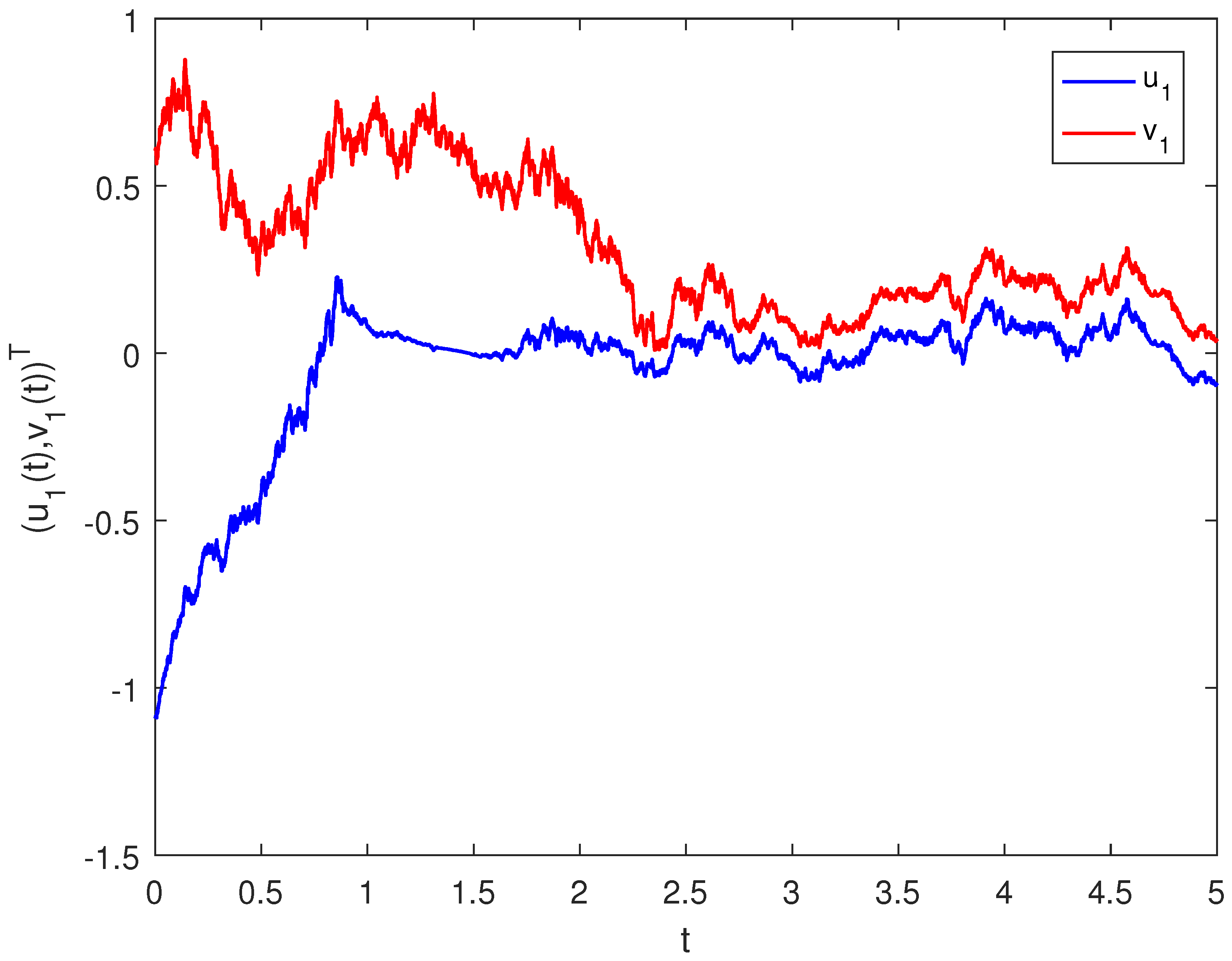
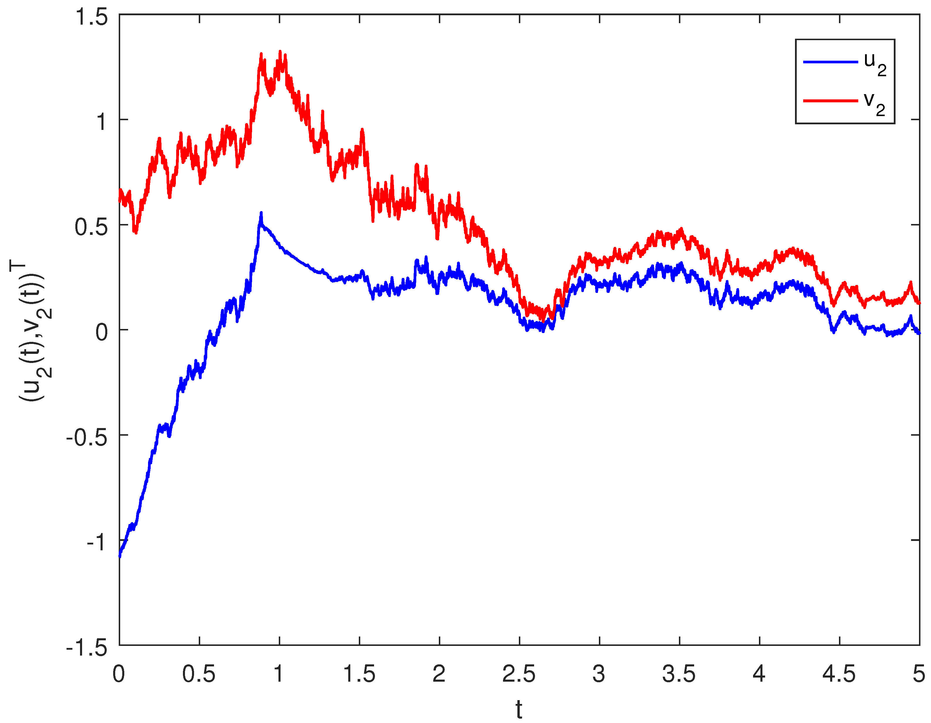
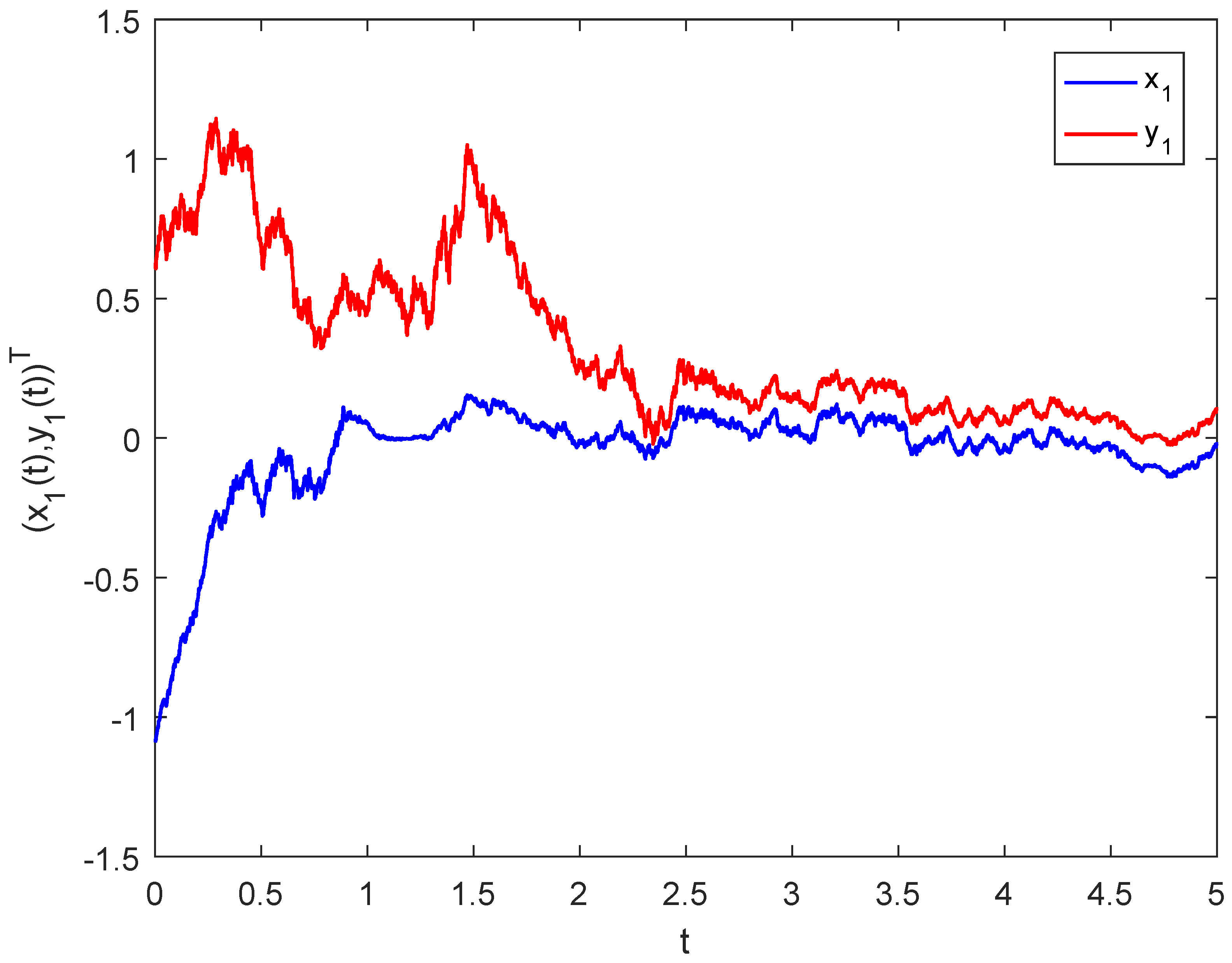
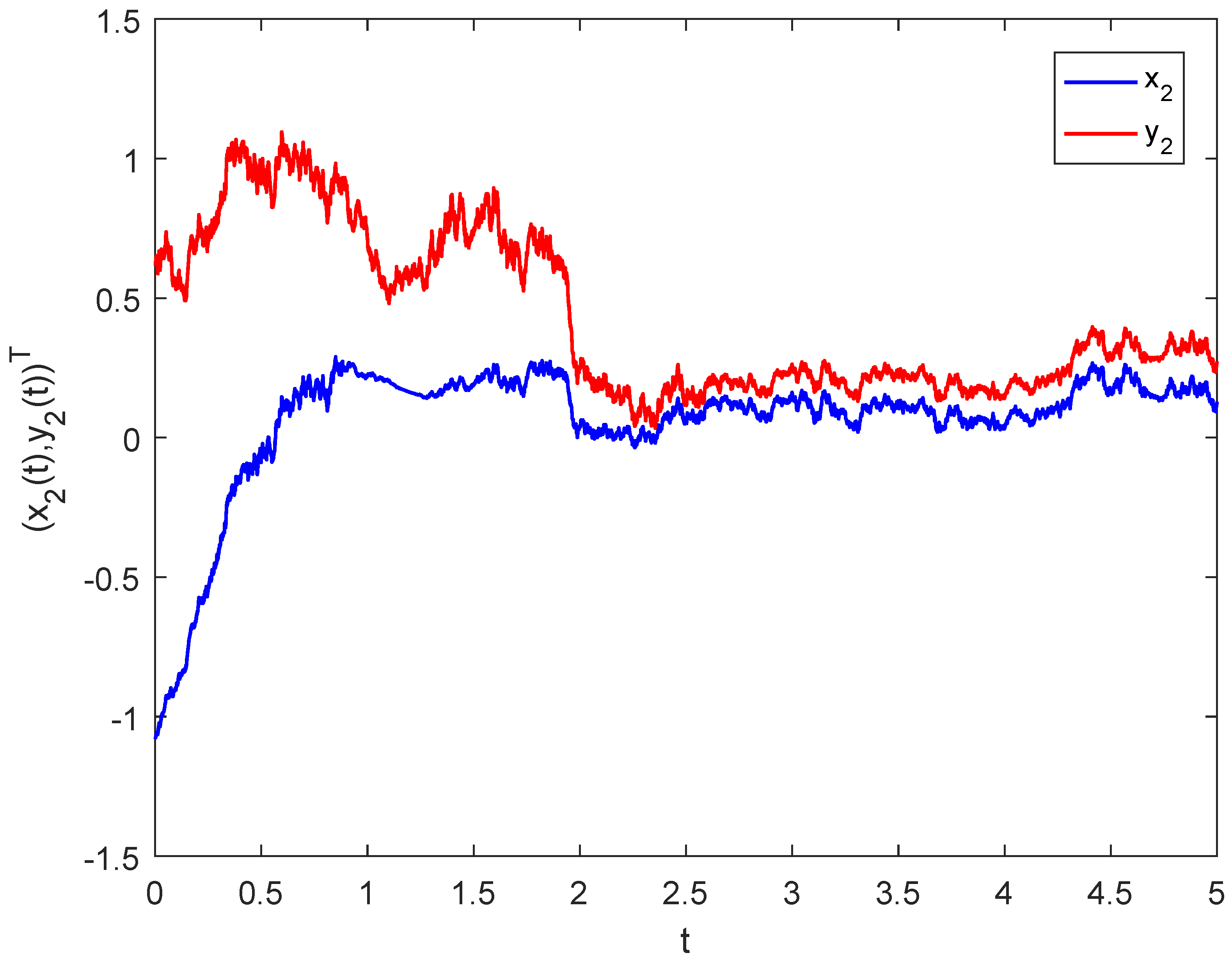
Theorem 2. 
Suppose that all conditions of Theorem 1 are satisfied. Then, system (3) has an equilibrium point which is stochastically globally asymptotically stable, provided that
2 a i + j = 1 n | b j i | L i 2 q i + j = 1 n k = 1 n M j L j | T i j k | q j + M i L i | T j i k | q i + j = 1 n k = 1 n M k L k | T i j k | q k + M i L i | T k j i | q i + j = 1 n | b i j | + | D i | + | β i | c L i + k = 1 n j = 1 n c k j 2 L ˜ i 2 < 0
and
2 α i + | D i | + | β i | c L i + k = 1 n j = 1 n d k j 2 L ˜ i 2 < 0 .
Proof. 
Due to Theorem 1, system (3) has a unique equilibrium point X * =   ( x 1 * , x 2 * , , x n * , y 1 * , y 2 * , , y n * ) T R 2 n . Let x ˜ i ( t ) = x i ( t ) x i * and y ˜ i ( t ) = y i ( t ) y i * . By (3), we have
d x ˜ i ( t ) = a i x ˜ i ( t ) d t + j = 1 n b i j f ˜ j ( x ˜ j ( q j t ) ) d t + j = 1 n k = 1 n T i j k f ˜ j ( x ˜ j ( q j t ) ) f ˜ k ( x ˜ k ( q k t ) ) d t + D i y ˜ i ( t ) d t + j = 1 n c i j g ˜ j ( x ˜ j ( t ) ) d W i ( t ) , d y ˜ i ( t ) = α i y ˜ i ( t ) d t + β i c f ˜ i ( x ˜ i ( t ) ) d t + j = 1 n d i j g ˜ j ( y ˜ j ( t ) ) d W i ( t ) ,
where
f ˜ j ( x ˜ j ( t ) ) = f j ( x ˜ j ( t ) + x j * ) f j ( x j * ) , g ˜ j ( y ˜ j ( t ) ) = g j ( y ˜ j ( t ) + y j * ) g j ( y j * ) .
Let
X ˜ = ( x ˜ , y ˜ ) = ( x ˜ 1 , x ˜ 2 , , x ˜ n , y ˜ 1 , y ˜ 2 , , y ˜ n )
and
V ( t , X ˜ ) = i = 1 n x ˜ i 2 ( t ) + y ˜ i 2 ( t ) + i = 1 n j = 1 n | b i j | q j t t 1 q j f ˜ j 2 ( x ˜ j ( s ) ) d s + i = 1 n j = 1 n k = 1 n | T i j k | q j t t 1 q j | x ˜ i ( s ) | f ˜ j 2 ( x ˜ j ( s ) ) d s + i = 1 n j = 1 n k = 1 n | T i j k | q k t t 1 q k | x ˜ i ( s ) | f ˜ k 2 ( x ˜ k ( s ) ) d s .
By (9), we get
V t ( t , X ˜ ) = i = 1 n j = 1 n | b i j | 1 q j f ˜ j 2 ( x ˜ j ( t ) ) f ˜ j 2 ( x ˜ j ( q j t ) ) + i = 1 n j = 1 n k = 1 n | T i j k | | x ˜ i ( t ) | q j f ˜ j 2 ( x ˜ j ( t ) ) | x ˜ i ( t ) | f ˜ j 2 ( x ˜ j ( q j t ) ) + i = 1 n j = 1 n k = 1 n | T i j k | | x ˜ i ( t ) | q k f ˜ k 2 ( x ˜ k ( t ) ) | x ˜ i ( t ) | f ˜ k 2 ( x ˜ k ( q k t ) )
and
V X ˜ ( t , X ˜ ) = 2 ( x ˜ 1 , x ˜ 2 , , x ˜ n , y ˜ 1 , y ˜ 2 , , y ˜ n ) , V X ˜ X ˜ ( t , X ˜ ) = 2 I 2 n × 2 n ,
where I 2 n × 2 n is a 2 n × 2 n identity matrix. It follows by (10), (11) and Definition 2 that
L V ( t , X ˜ ) = i = 1 n j = 1 n | b i j | 1 q j f ˜ j 2 ( x ˜ j ( t ) ) f ˜ j 2 ( x ˜ j ( q j t ) ) + i = 1 n j = 1 n k = 1 n | T i j k | | x ˜ i ( t ) | q j f ˜ j 2 ( x ˜ j ( t ) ) | u ˜ i ( t ) | f ˜ j 2 ( x ˜ j ( q j t ) ) + i = 1 n j = 1 n k = 1 n | T i j k | | x ˜ i ( t ) | q k f ˜ k 2 ( x ˜ k ( t ) ) | x ˜ i ( t ) | f ˜ k 2 ( x ˜ k ( q k t ) ) + 2 i = 1 n x ˜ i a i x ˜ i ( t ) + j = 1 n b i j f ˜ j ( x ˜ j ( q j t ) ) + j = 1 n k = 1 n T i j k f ˜ j ( x ˜ j ( q j t ) ) f ˜ k ( x ˜ k ( q k t ) ) + D i y ˜ i ( t ) + 2 i = 1 n y ˜ i α i y ˜ i ( t ) + β i c f ˜ i ( x ˜ i ( t ) ) + i = 1 n j = 1 n c i j g ˜ j ( x ˜ j ( t ) ) 2 + i = 1 n j = 1 n d i j g ˜ j ( y ˜ j ( t ) ) 2 .
Using the inequality a 2 + b 2 2 a b and (12), we get
L V ( t , X ˜ ) i = 1 n j = 1 n | b i j | 1 q j f ˜ j 2 ( x ˜ j ( t ) ) f ˜ j 2 ( x ˜ j ( q j t ) ) + i = 1 n j = 1 n k = 1 n | T i j k | | x ˜ i ( t ) | q j f ˜ j 2 ( x ˜ j ( t ) ) | x ˜ i ( t ) | f ˜ j 2 ( x ˜ j ( q j t ) ) + i = 1 n j = 1 n k = 1 n | T i j k | | x ˜ i ( t ) | q k f ˜ k 2 ( x ˜ k ( t ) ) | x ˜ i ( t ) | f ˜ k 2 ( x ˜ k ( q k t ) ) + i = 1 n ( 2 a i x ˜ i 2 ( t ) + j = 1 n | b i j | f ˜ j 2 ( x ˜ j ( q j t ) ) + j = 1 n | b i j | x ˜ i 2 ( t ) + j = 1 n k = 1 n | T i j k | | x ˜ i ( t ) | f ˜ j ( x ˜ j 2 ( q j t ) ) + f ˜ k 2 ( x ˜ k ( q k t ) ) + | D i | x ˜ i 2 ( t ) + | D i | y ˜ i 2 ( t ) ) + i = 1 n 2 α i y ˜ i 2 ( t ) + | β i | c L i x ˜ i 2 ( t ) + | β i | c L i y ˜ i 2 ( t ) + i = 1 n k = 1 n j = 1 n c k j 2 L ˜ i 2 x ˜ i 2 ( t ) + i = 1 n k = 1 n j = 1 n d k j 2 L ˜ i 2 y ˜ i 2 ( t ) i = 1 n [ 2 a i + j = 1 n | b j i | L i 2 q i + j = 1 n k = 1 n ( | T i j k | M j L j q j + | T j i k | M i L i q i ) + j = 1 n k = 1 n | T i j k | M k L k q k + | T k j i | M i L i q i + j = 1 n | b i j | + | D i | + | β i | c L i + k = 1 n j = 1 n c k j 2 L ˜ i 2 ] x ˜ i 2 ( t ) + i = 1 n 2 α i + | D i | + | β i | c L i + k = 1 n j = 1 n d k j 2 L ˜ i 2 y ˜ i 2 ( t ) .
It follows from (6), (7) and (13) that L V ( t , X ˜ ) < 0 . Therefore, L V ( t , X ˜ ) is negative definite. It is easy to see that V ( t , Z ˜ ) is positive definite. We claim that V ( t , Z ˜ ) has an infinitesimal upper bound. In fact, in view of assumption (H 1 ), we get
V ( t , X ˜ ) i = 1 n x ˜ i 2 ( t ) + y ˜ i 2 ( t ) + i = 1 n j = 1 n | b i j | q j t t L j 2 q j x ˜ j 2 ( s ) d s + i = 1 n j = 1 n k = 1 n | T i j k | q j t t L j 2 q j | x ˜ i ( s ) | x ˜ j 2 ( s ) d s + i = 1 n j = 1 n k = 1 n | T i j k | q k t t L k 2 q k | x ˜ i ( s ) | x ˜ k 2 ( s ) d s .
In view of Definition 3, there exists an infinitesimal upper bound of V ( t , X ˜ ) . It follows by (9) that
V ( t , X ˜ ) i = 1 n x ˜ i 2 ( t ) + y ˜ i 2 ( t ) .
Thus, V ( t , X ˜ ) + for | | X ˜ | | . Therefore, in view of Definition 4, V ( t , X ˜ ) is an infinite positive definite function for the second variable X ˜ . Based on Lemma 1, there is an equilibrium point of (3) which is stochastically globally asymptotically stable. □
We further study the properties of solutions of system (3) and discuss the estimation of the second moment.
Theorem 3. 
Suppose that (H 1 ) and (H 2 ) are satisfied. Furthermore, there exists a positive constant r i such that
a i = D i α i = r i .
Then, for any solution X = ( x 1 , x 2 , , x n , y 1 , y 2 , , y n ) T of system (3) that satisfies initial condition (4), we obtain that
E | x i ( t ) | 2 M 3 ˜ and E | y i ( t ) | 2 M 2 ˜ ,
where
M 1 ˜ = max 1 i n { 3 [ x i ( 0 ) + y i ( 0 ) ] 2 + 3 j = 1 n | b i j | M j + j = 1 n k = 1 n | T i j k | M j M k + | I i | + | β i | c M i 2 1 r i + 3 j = 1 n ( | c i j | + | d i j ) | N j 2 1 2 r i } ,
M 2 ˜ = max 1 i n 3 y i 2 ( 0 ) + 3 | β i | 2 c 2 M i 2 1 α i + 3 j = 1 n | d i j | N j 2 1 2 α i , M 3 ˜ = 2 M 1 ˜ + 2 M 2 ˜ .
Proof. 
By (3), we have
d x i ( t ) + d y i ( t ) + a i x i ( t ) d t + ( α i D i ) y i ( t ) d t = j = 1 n b i j f j ( x j ( q j t ) ) d t + j = 1 n k = 1 n T i j k f j ( x j ( q j t ) ) f k ( x k ( q k t ) ) d t + I i d t + β i c f i ( x i ( t ) ) d t + j = 1 n c i j g j ( x j ( t ) ) + j = 1 n d i j g j ( y j ( t ) ) d W i ( t ) .
Multiplying e r i t on both sides of (16) and using (15) yields
d e r i t x i ( t ) + e r i t y i ( t ) = e r i t [ j = 1 n b i j f j ( x j ( q j t ) ) d t + j = 1 n k = 1 n T i j k f j ( x j ( q j t ) ) f k ( x k ( q k t ) ) d t + I i d t + β i c f i ( x i ( t ) ) d t + j = 1 n c i j g j ( x j ( t ) ) + j = 1 n d i j g j ( y j ( t ) ) d W i ( t ) ] .
Integrating two sides of (17) on [ 0 , t ] , we get
x i ( t ) + y i ( t ) = e r i t [ x i ( 0 ) + y i ( 0 ) ] + 0 t e r i ( s t ) j = 1 n b i j f j ( x j ( q j s ) ) + j = 1 n k = 1 n T i j k f j ( x j ( q j s ) ) f k ( x k ( q k s ) ) + I i + β i c f i ( x i ( s ) ) d s + 0 t e r i ( s t ) j = 1 n c i j g j ( x j ( s ) ) + j = 1 n d i j g j ( y j ( s ) ) d W i ( s ) .
Thus,
| x i ( t ) + y i ( t ) | 2 3 e 2 r i t [ x i ( 0 ) + y i ( 0 ) ] 2 + 3 ( 0 t e r i ( s t ) [ j = 1 n b i j f j ( x j ( q j s ) ) + j = 1 n k = 1 n T i j k f j ( x j ( q j s ) ) f k ( x k ( q k s ) ) + I i + β i c f i ( x i ( s ) ) ] d s ) 2 + 3 0 t e r i ( s t ) j = 1 n c i j g j ( x j ( s ) ) + j = 1 n d i j g j ( y j ( s ) ) d W i ( s ) 2 3 [ x i ( 0 ) + y i ( 0 ) ] 2 + 3 j = 1 n | b i j | M j + j = 1 n k = 1 n | T i j k | M j M k + | I i | + | β i | c M i 2 1 e r i t r i + 3 0 t e r i ( s t ) j = 1 n c i j g j ( x j ( s ) ) + j = 1 n d i j g j ( y j ( s ) ) d W i ( s ) 2 .
Using the Schwarz inequality and It o ^ integration’s property, we get
E 0 t e r i ( s t ) j = 1 n c i j g j ( x j ( s ) ) + j = 1 n d i j g j ( y j ( s ) ) d W i ( s ) 2 = 0 t e 2 r i ( s t ) E j = 1 n c i j g j ( x j ( s ) ) + j = 1 n d i j g j ( y j ( s ) ) 2 d s j = 1 n ( | c i j | + | d i j ) | N j 2 1 e 2 r i t 2 r i .
Using (18) and (19) yields
E | x i ( t ) + y i ( t ) | 2 3 [ x i ( 0 ) + y i ( 0 ) ] 2 + 3 j = 1 n | b i j | M j + j = 1 n k = 1 n | T i j k | M j M k + | I i | + | β i | c M i 2 1 r i + 3 j = 1 n ( | c i j | + | d i j ) | N j 2 1 2 r i : = M 1 ˜ .
On the other hand, from the second equation of (3), we have
d e α i t y i ( t ) = e α i t β i c f i ( x i ( t ) ) d t + e α i t j = 1 n d i j g j ( y j ( t ) ) d W i ( t ) .
Integrating two sides of (21) on [ 0 , t ] , we get
y i ( t ) = y i ( 0 ) + 0 t e α i ( s t ) β i c f i ( x i ( s ) ) d s + 0 t e α i ( s t ) j = 1 n d i j g j ( y j ( s ) ) d W i ( s ) .
Using the above proof and (22), we derive
E | y i ( t ) | 2 3 y i 2 ( 0 ) + 3 | β i | 2 c 2 M i 2 1 α i + 3 j = 1 n | d i j | N j 2 1 2 α i : = M 2 ˜ .
From (20) and (23), we derive
E | x i ( t ) | 2 2 E | x i ( t ) + y i ( t ) | 2 + 2 E | y i ( t ) | 2 2 M 1 ˜ + 2 M 2 ˜ : = M 3 ˜
The proof of Theorem 3 is completed. □

4. Examples

Example 1. 
The following Hopfield-type stochastic networks with unsupervised Hebbian-type learning algorithms and proportional delays are given:
d u 1 ( t ) = 10 u 1 ( t ) d t + h 1 ( u 1 ( 1 3 t ) ) d t + h 2 ( u 2 ( 1 3 t ) ) d t + h 1 ( u 1 ( 1 3 t ) ) h 1 ( u 1 ( 1 3 t ) ) d t + h 1 ( u 1 ( 1 3 t ) ) + h 2 ( u 2 ( 1 3 t ) ) d t + h 2 ( u 2 ( 1 3 t ) ) h 1 ( u 1 ( 1 3 t ) ) d t + h 2 ( u 2 ( 1 3 t ) ) h 2 ( u 2 ( 1 3 t ) ) d t + 1 5 v 1 ( t ) d t + e 1 ( u 1 ( t ) ) d W 1 ( t ) , d v 1 ( t ) = 10 v 1 ( t ) d t + 1 2 h 1 ( u 1 ( t ) ) d t + e 1 ( v 1 ( t ) ) d W 1 ( t ) , d u 2 ( t ) = 10 u 2 ( t ) d t + h 1 ( u 1 ( 1 3 t ) ) d t + h 2 ( u 2 ( 1 3 t ) ) d t + h 1 ( u 1 ( 1 3 t ) ) h 1 ( u 1 ( 1 3 t ) ) d t + h 1 ( u 1 ( 1 3 t ) ) + h 2 ( u 2 ( 1 3 t ) ) d t + h 2 ( u 2 ( 1 3 t ) ) h 1 ( u 1 ( 1 3 t ) ) d t + h 2 ( u 2 ( 1 3 t ) ) h 2 ( u 2 ( 1 3 t ) ) d t + 1 5 v 2 ( t ) d t + e 2 ( u 2 ( t ) ) d W 1 ( t ) , d v 2 ( t ) = 10 v 2 ( t ) d t + 1 2 h 2 ( u 2 ( t ) ) d t + e 2 ( v 2 ( t ) ) d W 2 ( t ) ,
where
i , j , k = 1 , 2 , a i = α i = 10 , h 1 ( x ) = h 2 ( x ) = 1 10 tanh x , e 1 ( x ) = e 2 ( x ) = 1 20 tanh x , q i = 1 3 , I i = 0 ,
b i j = c i j = d i j = 1 , D i = 1 5 , c = 1 , β i = 1 2 , T i j k = 1 , L j = M j = 1 10 , L ˜ j = N j = 1 20 .
After a simple calculation, we have
μ = max 1 i n L i a i j = 1 n b j i + j = 1 n k = 1 n ( T k j i + T k i j ) M j + | D i | c | β i | α i 0.12 < 1 ,
2 a i + j = 1 n | b j i | L i 2 q i + j = 1 n k = 1 n | T i j k | M j L j q j + | T j i k | M i L i q i + j = 1 n k = 1 n | T i j k | M k L k q k + | T k j i | M i L i q i + j = 1 n | b i j | + | D i | + | β i | c L i + k = 1 n j = 1 n c k j 2 L ˜ i 2 17.04 < 0
and
2 α i + | D i | + | β i | c L i + k = 1 n j = 1 n d k j 2 L ˜ i 2 = 13.35 < 0 .
Thus, all conditions of Theorems 1 and 2 are satisfied and for system (24) there exists a globally asymptotically stable equilibrium X * = ( 0 , 0 , 0 , 0 ) T . Figure 1 and Figure 2 show that system (24) has an equilibrium point which is stochastically globally asymptotically stable. Figure 1 and Figure 2 show that the solution of (24) approaches equilibrium at X * = ( 0 , 0 , 0 , 0 ) T .
Example 2. 
To further verify the results of Theorems 1 and 2, according to system (3), we provide the following example:
d x 1 ( t ) = 12 x 1 ( t ) d t + h 1 ( x 1 ( 1 5 t ) ) d t + h 2 ( x 2 ( 1 5 t ) ) d t + h 1 ( x 1 ( 1 5 t ) ) h 1 ( x 1 ( 1 5 t ) ) d t + h 1 ( x 1 ( 1 5 t ) ) + h 2 ( x 2 ( 1 5 t ) ) d t + h 2 ( x 2 ( 1 5 t ) ) h 1 ( x 1 ( 1 5 t ) ) d t + h 2 ( x 2 ( 1 5 t ) ) h 2 ( x 2 ( 1 5 t ) ) d t + 1 6 y 1 ( t ) d t + e 1 ( x 1 ( t ) ) d W 1 ( t ) , d y 1 ( t ) = 12 y 1 ( t ) d t + 1 4 h 1 ( x 1 ( t ) ) d t + e 1 ( y 1 ( t ) ) d W 1 ( t ) , d x 2 ( t ) = 12 x 2 ( t ) d t + h 1 ( x 1 ( 1 5 t ) ) d t + h 2 ( x 2 ( 1 5 t ) ) d t + h 1 ( x 1 ( 1 5 t ) ) h 1 ( x 1 ( 1 5 t ) ) d t + h 1 ( x 1 ( 1 5 t ) ) + h 2 ( x 2 ( 1 5 t ) ) d t + h 2 ( x 2 ( 1 5 t ) ) h 1 ( x 1 ( 1 5 t ) ) d t + h 2 ( x 2 ( 1 5 t ) ) h 2 ( x 2 ( 1 5 t ) ) d t + 1 6 y 2 ( t ) d t + e 2 ( x 2 ( t ) ) d W 1 ( t ) , d y 2 ( t ) = 12 y 2 ( t ) d t + 1 4 h 2 ( x 2 ( t ) ) d t + e 2 ( y 2 ( t ) ) d W 2 ( t ) ,
where
i , j , k = 1 , 2 , a i = α i = 12 , h 1 ( x ) = h 2 ( x ) = 1 15 tanh x , e 1 ( x ) = e 2 ( x ) = 1 40 tanh x , q i = 1 5 , I i = 0 ,
b i j = c i j = d i j = 1 , D i = 1 6 , c = 1 , β i = 1 4 , T i j k = 1 .
From the expressions of h 1 , h 2 , e 1 and e 2 , we obtain
L j = M j = 1 15 , L ˜ j = N j = 1 40 , j = 1 , 2 .
Thus, assumptions (H 1 ) and (H 2 ) hold. After a simple calculation, we have
μ = max 1 i n L i a i j = 1 n b j i + j = 1 n k = 1 n ( T k j i + T k i j ) M j + | D i | c | β i | α i 0.014 < 1 ,
2 a i + j = 1 n | b j i | L i 2 q i + j = 1 n k = 1 n | T i j k | M j L j q j + | T j i k | M i L i q i + j = 1 n k = 1 n | T i j k | M k L k q k + | T k j i | M i L i q i + j = 1 n | b i j | + | D i | + | β i | c L i + k = 1 n j = 1 n c k j 2 L ˜ i 2 21.15 < 0
and
2 α i + | D i | + | β i | c L i + k = 1 n j = 1 n d k j 2 L ˜ i 2 = 23.82 < 0 .
Therefore, all conditions of Theorems 1 and 2 are satisfied and system (25) has a globally asymptotically stable equilibrium X * = ( 0 , 0 , 0 , 0 ) T . From Figure 3 and Figure 4, it is easy to see that system (25) has an equilibrium point at X * = ( 0 , 0 , 0 , 0 ) T which is stochastically globally asymptotically stable.

5. Conclusions

By using the Lyapunov functional method and stochastic analysis techniques, we derive some sufficient conditions to ensure the global asymptotic stability of system (3). We also give an estimation of the second moment for the solution of system (3). An example is given to demonstrate the correctness of the obtained results.
There are still many issues worth further research in system (3), such as network models with pulse structures, networks on time scales, networks with fuzzy terms, and so on.

Author Contributions

Methodology, X.W. and X.C.; Writing—original draft, F.Z. All authors have read and agreed to the published version of the manuscript.

Funding

This work was supported by the National Natural Science Foundation of China (No. 11971197).

Data Availability Statement

Data are contained within the article.

Acknowledgments

The authors would like to thank the editor and the referees for their valuable comments and suggestions that improved the quality of our paper.

Conflicts of Interest

The authors declare no conflict of interest.

References

  1. Gopalsamy, K. Learning dynamics in second order networks. Nonlinear Anal. Real World Appl. 2007, 8, 688–698. [Google Scholar] [CrossRef]
  2. Huang, Z.; Feng, C.; Mohamad, S.; Ye, J. Multistable learning dynamics in second-order neural networks with time-varying delays. Int. J. Comput. Math. 2011, 88, 1327–1346. [Google Scholar] [CrossRef]
  3. Gopalsamy, K. Learning dynamics and stability in networks with fuzzy syapses. Dyn. Syst. Appl. 2006, 15, 657–671. [Google Scholar]
  4. Chu, D.; Nguyen, H. Constraints on Hebbian and STDP learned weights of a spiking neuron. Neural Netw. 2021, 135, 192–200. [Google Scholar] [CrossRef]
  5. Chen, J.; Huang, Z.; Cai, J. Global Exponential Stability of Learning-Based Fuzzy Networks on Time Scales. Abstr. Appl. Anal. 2015, 2015, 83519. [Google Scholar] [CrossRef]
  6. Huang, Z.; Raffoul, Y.; Cheng, C. Scale-limited activating sets and multiperiodicity for threshold-linear networks on time scales. IEEE Trans. Cybern. 2014, 44, 488–499. [Google Scholar] [CrossRef]
  7. Cao, J.; Liang, J.; Lam, J. Exponential stability of high order bidirectional associative memory neural networks with time delays. Phys. D 2004, 199, 425–436. [Google Scholar] [CrossRef]
  8. Kosmatopoulos, E.; Polycarpou, M.; Christodoulou, M.; Ioannou, P. High order neural network structures for identification of dynamical systems. IEEE Trans. Neural Netw. 1995, 6, 422–431. [Google Scholar] [CrossRef]
  9. Zhang, Z.; Liu, K. Existence and global exponential stability of a periodic solution to interval general bidirectional associative memory (BAM) neural networks with multiple delays on time scales. Neural Netw. 2011, 24, 427–439. [Google Scholar] [CrossRef]
  10. Kamp, Y.; Hasler, M. Recursive Neural Networks for Associative Memory; Wiley: New York, NY, USA, 1990. [Google Scholar]
  11. Liu, Y.; Wang, Z.; Liu, X. An LMI approach to stability analysis of stochastic high-order Markovian jumping neural networks with mixed time delays. Nonlinear Anal. Hybrid Syst. 2008, 2, 110–120. [Google Scholar] [CrossRef]
  12. Xing, J.; Peng, C.; Cao, Z. Event-triggered adaptive fuzzy tracking control for high-order stochastic nonlinear systems. J. Frankl. Inst. 2022, 359, 6893–6914. [Google Scholar] [CrossRef]
  13. Wang, J.; Liu, Z.; Chen, C.; Zhang, Y. Event-triggered fuzzy adaptive compensation control for uncertain stochastic nonlinear systems with given transient specification and actuator failures. Fuzzy Sets Syst. 2019, 365, 1–21. [Google Scholar] [CrossRef]
  14. Yang, G.; Li, X.; Ding, X. Numerical investigation of stochastic canonical Hamiltonian systems by high order stochastic partitioned Runge–Kutta methods. Commun. Nonlinear Sci. Numer. Simul. 2021, 94, 105538. [Google Scholar] [CrossRef]
  15. Wang, H.; Zhu, Q. Output-feedback stabilization of a class of stochastic high-order nonlinear systems with stochastic inverse dynamics and multidelay. Int. J. Robust Nonlinear Control. 2021, 13, 5580–5601. [Google Scholar] [CrossRef]
  16. Xie, X.; Duan, N.; Yu, X. State-Feedback Control of High-Order Stochastic Nonlinear Systems with SiISS Inverse Dynamics. IEEE Trans. Autom. Control. 2011, 56, 1921–1936. [Google Scholar]
  17. Fei, F.; Jenny, P. A high-order unified stochastic particle method based on the Bhatnagar-Gross-Krook model for multi-scale gas flows. Comput. Phys. Commun. 2022, 274, 108303. [Google Scholar] [CrossRef]
  18. Mao, X. Stochastic Differential Equations and Applications; Horwood: Buckinghamshire, UK, 1997. [Google Scholar]
  19. Forti, M.; Tesi, A. New conditions for global stability of neural networks with application to linear and quadratic programming problems. IEEE Trans. Circuits Syst. 1995, 42, 354–366. [Google Scholar] [CrossRef]
Figure 1. Simulation results for the solution ( u 1 ( t ) , v 1 ( t ) ) T in system (24).
Mathematics 11 04755 g001
Figure 2. Simulation results for the solution ( u 2 ( t ) , v 2 ( t ) ) T in system (24).
Mathematics 11 04755 g002
Figure 3. Simulation results for the solution ( x 1 ( t ) , y 1 ( t ) ) T in system (25).
Mathematics 11 04755 g003
Figure 4. Simulation results for the solution ( x 2 ( t ) , y 2 ( t ) ) T in system (25).
Mathematics 11 04755 g004
Disclaimer/Publisher’s Note: The statements, opinions and data contained in all publications are solely those of the individual author(s) and contributor(s) and not of MDPI and/or the editor(s). MDPI and/or the editor(s) disclaim responsibility for any injury to people or property resulting from any ideas, methods, instructions or products referred to in the content.

