1. Introduction
Inland waterways transportation plays a pivotal role in facilitating the efficient movement of goods and passengers across vast geographical regions. Serving as a valuable alternative to road and rail transport, inland waterways offer numerous advantages, including cost savings, reduced ecological impact, heightened environmental compatibility, and the capacity to handle substantial cargo volumes. The global network of inland navigation systems spans an estimated length of over 650,000 km, with projections indicating further expansion in the years to come [
1]. These waterways serve as a critical linchpin within the multifaceted realm of multimodal transportation systems, thus seamlessly connecting industrially productive heartland regions with international gateways. This interconnectedness is instrumental in ensuring the maintenance of competitive transportation costs [
2]. To illustrate, the United States boasts an extensive network of over 25,000 m of inland waterways, which is responsible for transporting approximately 14% of the nation’s entire domestic freight volume, thereby translating into an impressive annual cargo throughput exceeding 600 million tons [
3]. In Europe, an intricate web of more than 23,000 m of interlinked waterways seamlessly weaves through industrial hubs and urban centers, thereby facilitating the transportation of an excess of 500 million tons of goods each year [
4], with discernibly promising growth prospects on the horizon [
5]. Moreover, given the inherent advantages of inland waterways transportation over road and other modes of transportation, the redirection of freight towards inland waterway transport has earned fervent support from the European Commission. The Commission has proactively undertaken measures to champion the advancement of inland waterway transport through the Navigation and Inland Waterway Action and Development in Europe (NAIADES) program. This strategic initiative is geared toward not only endorsing, but actively fostering the transition, thus mitigating the pressures and congestion associated with conventional modes of transportation [
6]. What is more, the deployment of a single vessel, with the capacity to supplant more than 100 trucks, holds the potential to ameliorate congestion issues and reduce the incidence of road network accidents. The Netherlands, which is strategically situated at the confluence of several pivotal European rivers, serves as a prime exemplar in this regard, accounting for a substantial 58% share of all European freight transportation enterprises [
7]. In 2018, the Dutch inland waterway transportation network encompassed a vast expanse, spanning over 6297 km of navigable inland water routes and hosting a remarkable 34.85% share of total freight transport measured in tonne-kilometres [
7].
However, despite the advantages offered by inland waterway transportation, it is not without its challenges. Pollution arising from vessel emissions poses a significant threat to the ecosystems and communities along these water routes. Furthermore, the escalating fuel prices have imposed colossal cost pressures on shipping companies. And beyond the extended durations of travel, which are primarily attributed to relatively sparse network coverage, a substantial impediment in the domain of freight transportation is the profound unpredictability associated with arrival times. A significant source of this uncertainty emanates from the presence of locks within the waterway systems. These locks introduce pivotal bottlenecks along the river arteries, and due to the paucity of accessible information, the precise passage time for a skipper navigating through such a lock remains obscured from the awareness of fellow skippers, which consequently eludes precise prediction [
8].
To move towards a greener and more sustainable future, shipping companies operating in inland waterway transportation must align their practices with environmental preservation objectives. This necessitates making informed optimization decisions that encompass various factors, including sailing speeds, to minimize resource consumption, reduce emissions, and ultimately lower overall costs [
9]. Particularly, for segments of navigation that involve time windows, shipping companies need to thoroughly consider the sailing schedule for the entire route, thus avoiding unnecessary waiting times and optimizing operational efficiency to minimize total costs while meeting the defined time constraints.
In this paper, we present mathematical models with the objective of facilitating optimal decision making for inland shipping companies in their pursuit of cost minimization, all while ensuring on-time arrival at the port of discharge. Our study encompasses single-lane routes, as well as alternating routes with two-lane segments, thereby incorporating time windows and speed constraints. Specifically, our investigation addresses the following research questions:
What are the optimal sailing speeds for the flow of traffic in one-way and alternating one-way inland shipping routes, considering the time window constraints of single-lane segments and the prescribed arrival time at the port of discharge, in order to minimize the overall expenses incurred by shipping companies?
What are the optimal time windows for the one-way segments, taking into account the time window constraints of single-lane segments and the prescribed arrival time at the port of discharge, in order to minimize the aggregate expenses incurred by shipping companies?
On the one hand, by meticulously considering time window restrictions in single-lanes to determine the optimal sailing speeds of vessels, we ensure their punctual arrival while markedly curbing fuel consumption. This not only fine-tunes operational logistics for shipping enterprises, thus facilitating substantial cost abatements, but also champions heightened fuel efficiency and a tangible reduction in carbon emissions within maritime transportation. The other facet involves pinpointing the optimal time window for vessels to navigate the single-lane segment, thus aiding vessels in smoothly transiting through the designated waterways within stipulated time windows. This strategic approach serves to attenuate extended waiting durations, which are a consequence of missing the optimal entry window. It, in turn, leads to a reduction in vessel idle times and a significant curtailment of carbon emissions during these periods of inactivity.
To tackle these research questions, we initially introduce a sophisticated nonlinear optimization model characterized by its intricate nature and the complexity of problem-solving it entails. Subsequently, advanced mathematical techniques are employed to transform the initial model into an integer programming (IP) model. This conversion allows us to leverage off-of-shelf optimization solvers for effectively solving the IP model. Finally, we conduct a series of comprehensive experiments and perform comparisons with three strategies to validate the optimization effectiveness of our proposed research model.
Research Contributions
Theoretical contributions: The present study addresses a notable research gap by focusing on the optimal selection of streaming speed in each leg and the time window constraints in one-way segments. Importantly, this specific aspect has been overlooked in the existing scholarly literature. To the best of our understanding, this research represents a pioneering endeavor in establishing mathematical models that take into account various types of waterways and the time windows in single-lane channels. The main objective of these models is to assist shipping companies in their timely reaching of the port of discharge while minimizing operational costs in order to achieve sustainable and environmentally friendly development.
Practical contributions: The proposed approach employs an IP model to determine the optimal decisions for shipping companies. Through rigorous experiments and the comparison of three strategies, our model has demonstrated superior optimization performance, thereby providing valuable decision-making insights for shipping companies. This research contributes significant practical implications to the realm of inland shipping by offering insights into the development of optimal strategies for shipping companies. Particularly, considering the unique characteristics and complexities of inland shipping, this study comprehensively takes into account the time window issue in single-lane channels, thereby providing valuable reference and guidance for shipping companies. The obtained results carry practical significance in fostering sustainable growth within the inland shipping industry and facilitating its alignment with environmental regulations.
Overall, this study presents a novel and robust approach to optimize the decision-making process in inland shipping, thus bridging the research gap in the existing literature and offering practical guidance for shipping companies seeking to minimize costs while ensuring timely arrival at the port of discharge.
The rest of the paper is organized as follows.
Section 2 reviews the existing literature.
Section 3 describes the research problem in detail and develops the mathematical model.
Section 4 proposes solution methods for addressing the initial proposed model.
Section 5 proposes three benchmark strategies.
Section 6 conducts experiments. Finally, conclusions are drawn in
Section 8.
2. Literature Review
We review two streams of literature closely related to our study: (i) emissions from inland waterways and (ii) optimal decisions in inland shipping.
2.1. Emissions from Inland Waterways
Ship emissions are widely recognized as the third most significant source of pollution, thereby surpassing industrial waste gases and automobile exhaust [
10]. Presently, traditional diesel remains the principal propulsion system for inland waterway ships, thus resulting in the generation of substantial quantities of oily sewage and hazardous exhaust gases during navigation and port entry. These emissions contain detrimental substances such as
and
. With the escalating demand for inland shipping, pollutant emissions have witnessed a year-on-year increase [
11,
12,
13]. For example, according to statistical data, ship and port emissions in the Yangtze River Delta region contribute approximately 28% to the national total of air pollutants. The Shanghai Port, in particular, accounts for about 12% of the city’s SO
2 emissions, 9% of
emissions, and 5% of PM2.5 emissions [
14]. Consequently, ship emission management has once again become a significant topic on the agenda. To effectively address pollution from inland shipping, the shipping industry has put forth numerous green innovative measures to promote its sustainable development. Among these initiatives, the all-electric ship (AES) stands out as a prominent technology. Currently, traditional diesel-powered vessels are gradually being replaced by AESs, thus enabling them to achieve reduced emissions, optimized energy allocation, and heightened operational efficiency [
15,
16]. In recent years, researchers also have conducted studies considering the impact of ship emissions in inland shipping on the regional economy and environment, thereby aligning their work with emission regulations and measures issued by international organizations and local governments. In 2011, the proposal of Directive 2009/30/EC brought changes to the fuel quality of inland vessels, thus resulting in improved air quality along rivers by reducing the total deposition of polycyclic aromatic hydrocarbons (PAHs) [
17,
18]. Additionally, Blasing et al. [
19] conducted a comprehensive investigation into the spatiotemporal dynamics of black carbon (BC) soil deposition resulting from inland shipping activities. Their findings elucidated that the implementation of sulfur control measures in marine diesel has yielded a notable reduction of approximately 30% in BC deposition attributed to inland shipping. Furthermore, as the paradigm of green shipping gains prominence, the shipping industry is increasingly focusing on clean energy alternatives and technological advancements for ships. This emergent discourse has garnered escalating attention within the industry. In their insightful study on mitigating oil pollution stemming from ship spills, Wan and Chen [
20] asserted the imperative of enhancing and advancing sustainable clean technologies. Therefore, against this backdrop, shipping companies are diligently considering environmental conservation and promoting green development as pivotal factors in their decision-making processes. Particularly, the introduction of pertinent policies and regulations serves as a catalyst, thus compelling these companies to optimize navigation speeds and routes to mitigate emissions, thereby accomplishing sustainable development objectives while concurrently reducing costs.
2.2. Optimal Decisions in Inland Shipping
Given the significance of waterway transportation, there has been considerable attention devoted to optimizing inland waterways to minimize the total cost, especially the optimization of the streaming speed. Not only does it impact the duration of voyages, but also it bears direct relevance to fuel cost, carbon emissions, and other environmental concerns [
21,
22]. Extensive studies have been conducted in this area. The work of Norstad et al. [
23] explored speed optimization problems for a single route while considering time windows. The work of Ronen [
24] investigated the determination of sailing speed and fleet size to minimize annual operating costs under different fuel prices. While sailing speed is the primary factor influencing energy consumption, it is essential to also consider other factors, such as the navigational environment. The authors in Fan et al. [
25] developed a ship energy efficiency model that incorporates multiple influencing factors, including cargo amount, sailing speed, and navigational environment. The model’s effectiveness was verified by comparing simulated results with actual collected data. Additionally, they studied the relationship between energy efficiency operation indices (EEOIs), energy consumption, cargo amount, sailing speed, and environmental factors. The intricate navigational conditions encountered by inland ships distinguish their speed optimization practices from those of ocean-going vessels. The authors in Sun et al. [
26] conducted an investigation on the EEOIs for inland ships under both calm water scenarios and actual navigation conditions. Their findings revealed that, apart from sailing speed, environmental factors play a significant role in influencing the energy efficiency of inland ships. Building upon data collected from real-life inland ship operations, Yin et al. [
27] conducted a comprehensive analysis of the correlation between environmental factors (such as water speed, wind speed, and water depth) and energy consumption. They employed clustering algorithms to partition the waterway, thereby identifying distinct regional characteristics in the navigational environment of the Yangtze River. Notably, water speed and water depth emerged as the primary influencing factors affecting energy consumption. In another study, Yuan et al. [
28] employed the k-means clustering method to delineate routes through the extensive analysis of big data. Subsequently, they proposed an optimization model for ship energy efficiency, thereby enabling the determination of optimal engine speeds for each segment of the journey. In addition, Farjana et al. [
29] presented a sophisticated mathematical model using multicommodity, multiperiod, mixed-integer linear programming. The objective is to effectively manage operations at inland waterway ports while minimizing the overall cost of the supply chain. This involved various strategic decisions, such as the tripwise assignment of towboats and barges, along with midterm supply chain considerations like inventory management [
30].
However, optimizing speed in the context of complex, nonlinear problems presents an intricate challenge, which is characterized by high computational costs. To tackle these nonlinear speed optimization issues, several advanced and efficient optimization algorithms have been introduced. The work of Tang et al. [
31] employed the particle swarm algorithm to address multiobjective speed optimization problems, thereby carefully selecting optimal engine speeds based on the resulting nondominated solutions and effectively balancing economic and safety requirements. In a bid to solve the dual-objective model that aims to minimize operational costs while maximizing customer satisfaction, Peng et al. [
32] introduced an improved algorithm based on the nondominated genetic algorithm. Their approach, incorporating fast nondominated sorting and an enhanced crowding distance operator, successfully managed multiple constraints in each generation and exhibited impressive convergence properties. The authors in Tu et al. [
33] proposed a speed optimization approach for coastal bulk carriers, thereby utilizing a multiobjective genetic algorithm to determine the most fuel-efficient speeds by considering the ship–engine–propeller relationship. Their findings demonstrated that expanding the range of low-load operation for the main engine and increasing voyage time contribute to reduced fuel consumption for the target vessels. In the domain of speed optimization, the commonly used penalty function approach employed for nonlinear constraint handling can exhibit limitations, thus requiring large penalty coefficients under certain conditions to attain optimal solutions and potentially leading to ill-conditioning and the Maratos effect, which hinder convergence. To overcome these issues, Wei et al. [
34] introduced an innovative heuristic algorithm known as ALDE for solving speed optimization problems in inland waterway shipping. The ALDE algorithm seamlessly combines the strengths of enhanced Lagrange functions and differential evolution, thus requiring fewer control parameters and offering automatic penalty and Lagrange multiplier updates, which mitigate the issues associated with penalty function methods, such as ill-conditioning and the Maratos effect. The utilization of enhanced Lagrange functions in conjunction with evolutionary algorithms has been explored in recent research.
In
Table 1, we have compiled a list of important literature regarding the emission problem of inland water transportation.
In general, inland waterway transportation has garnered increasing scholarly attention due to its pivotal role in the field of transportation and logistics. Particularly with the growing recognition of green development and sustainable principles by numerous nations, emissions issues in inland waterway transportation have received heightened scrutiny. Relevant organizations and governments have implemented policies to guide shipping companies toward green development practices. Against this backdrop, optimal decision making for shipping companies, particularly in the realm of speed optimization, becomes crucial. However, inland waterway transportation possesses unique characteristics and complexities compared to maritime transportation. For instance, shipping companies must consider factors such as single and dual waterway routes and time windows. To our knowledge, despite the increasing research attention dedicated to emission concerns in inland waterway transportation, there remains a conspicuous dearth of comprehensive studies addressing the optimization of vessel speed and the determination of ideal entry time windows for diverse categories of waterway routes. This void is particularly noticeable in the context of alternating single-lane and dual-lane navigation routes, where shipping companies grapple with the intricate decision-making processes related to the most favorable sailing speeds and the optimal entry time windows for single-lane segments. Hence, our research addresses the need by proposing an IP model for determining the optimal speed for various waterway types and selecting the optimal time window for entering single lane channels. The ultimate objective is to enable the timely arrival at the port of discharge while minimizing operational costs, thus actualizing green and sustainable development for shipping companies.
3. Problem Description and Model Development
Inland water transportation holds profound significance as a pivotal component of regional logistics networks, thus facilitating the movement of substantial volumes of cargo. Within this context, when compared to railways and highways, inland water transportation emerges as the most economically viable alternative, thereby boasting transport capacities that surpass those of its counterparts by up to 17 times [
35]. Nonetheless, the industry confronts several challenges, including insufficient automation and an overdependence on diesel-powered systems [
25]. Notably, among these issues, the emission of pollutants resulting from fuel combustion stands out. Such emissions directly degrade air quality for those residing in the vicinity of waterways, while also contributing significantly to various environmental concerns—most notably to global warming.
Conversely, the escalating costs of diesel in recent years have precipitated a larger proportion of fuel expenses within the overall operational outlays of shipping vessels. To alleviate this burden and mitigate emissions, reducing fuel consumption assumes paramount importance. With this goal in mind, inland waterway shipping companies are actively seeking effective methodologies. As a result, the optimization of ship speeds has garnered considerable attention, owing to its efficacy in curbing fuel consumption and conserving energy resources.
In this study, we consider sailing speed optimization with time windows for the inland water transportation of bulk carriers. The bulk carrier travels from the port of departure at time to the port of discharge, thus passing through the mainstream and tributaries. The vessel needs to arrive at the port of discharge within the time window to carry out its unloading operations. If the vessel arrives at the port of discharge earlier than , it has to wait until to carry out its unloading operations. The vessel is not allowed to arrive at the port of discharge later than .
3.1. One-Way Segments and Two-Way Segments
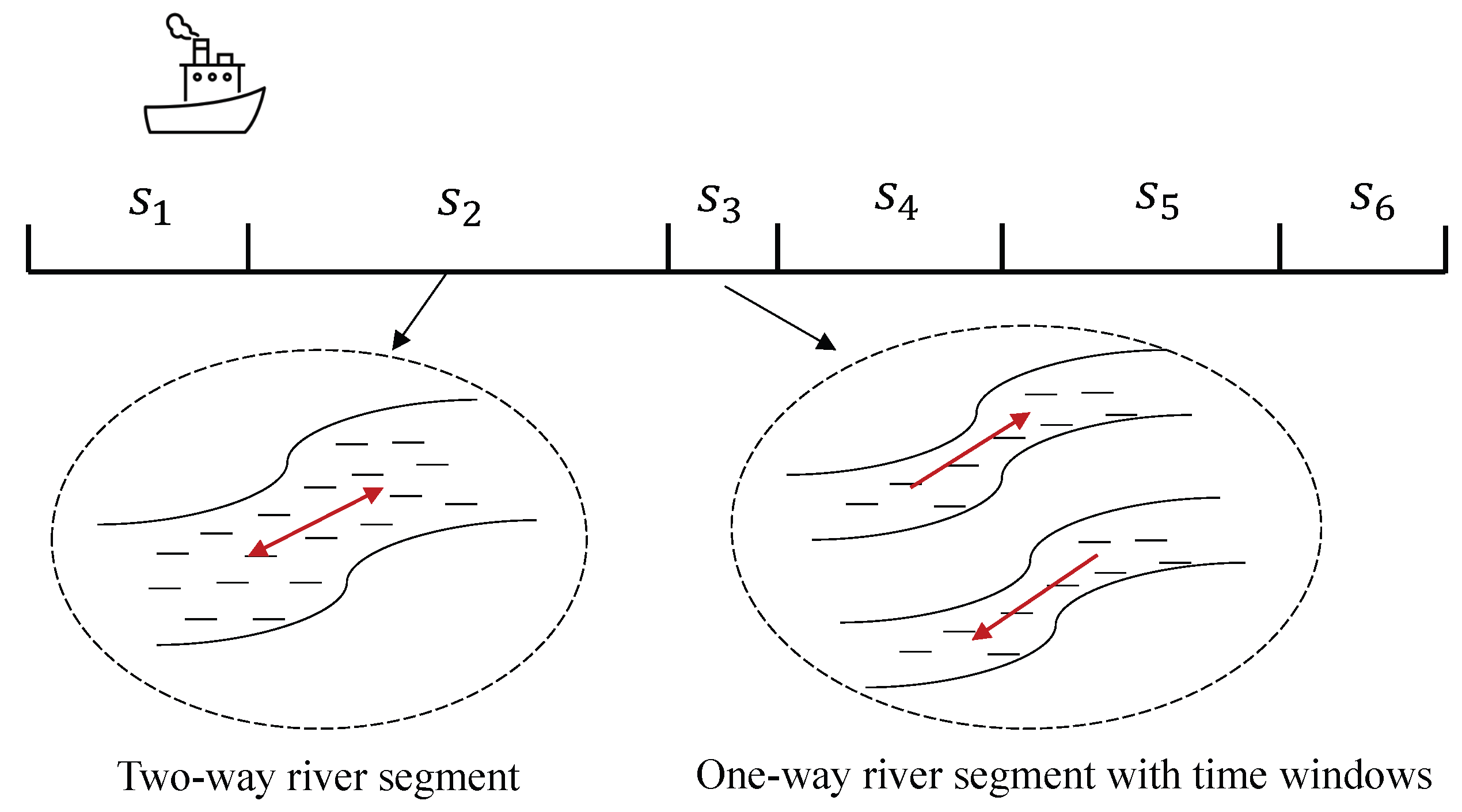
Based on the type of rivers (e.g., the mainstream and tributaries) and the restriction of the sailing speed, the sailing route of inland water transportation can be divided into many sailing segments as shown in
Figure 1. We use
I to denote sailing segments, and
refers to a particular sailing segment. For example, there are six sailing segments in
Figure 1. We use
to denote the length of the sailing segment
i. Most of the sailing segments are wide enough to allow for two-way sailing, i.e., vessels can travel in both directions in this channel at the same time. Some of the sailing segments are so narrow that vessels can only pass in one direction at a time, e.g., the third sailing segment in
Figure 1. Therefore, there is a fixed time window for this sailing segment. For example, vessels can travel from upstream to downstream from 00:00 to 11:00 and can travel from downstream to upstream from 15:00 to 20:00. Note that there is a 4 h gap between sailing direction changes, which is the time set aside to clear the vessel from the previous time period. We use
and
to denote the set of one-way sailing segments and the set of two-way sailing segments, respectively. And we have
. The sailing speed for each sailing segment
i is
, which is a decision variable. For the one-way sailing segment
, the sailing speed is within a maximum limit of
and a minimum limit of
, that is,
,
. For the two-way sailing segment
, the sailing speed only has a maximum limit of
, that is,
,
.
Without a loss of generality, we make the following assumptions to simplify the model formulation.
Assumption 1. The first segment is a two-way segment. If the first segment is a one-way segment, we can insert a ”dummy” two-way segment with a length of 0 before the first segment.
Assumption 2. The last segment is a two-way segment. If the last segment is a one-way segment, we can insert a “dummy” two-way segment with a length of 0 after the last segment.
Assumption 3. Each two-way segment (except the last one) is followed by a one-way segment. If a two-way segment is followed by another two-way segment with a different sailing speed limit, we can insert a ”dummy” one-way segment with a length of 0 and a time window from 00:00 to 24:00 between the two two-way segments.
Assumption 4. Each one-way segment is followed by a two-way segment. If a one-way segment is followed by another one-way segment with different sailing speed limits or a different time window, we can insert a ”dummy” two-way segment with a length of 0 between the two one-way segments.
Because of the above four assumptions, is always an odd number: segments 2, 4,…, are one-way, and segments 1, 3,…, are two-way, i.e., and .
3.2. Time Windows of the One-Way Direction Segments
If the vessel can enter a one-way segment i from 00:00 to 11:00 in a day, then the set of time windows for the vessel to enter the segment is . If the vessel can enter a one-way segment i from 00:00 to 03:30 or from 12:00 to 15:30 in a day, then the set of time windows for the vessel to enter the segment is . Although there are an infinite number of elements in a set of time windows, we only need to consider the ones that are no later than . Therefore, for each one-way segment , the number of time windows to consider is denoted by , and the kth time window is denoted by , , .
3.3. Costs
The vessel operator aims to minimize the total costs, including the chartering cost and fuel cost. The chartering cost per hour is denoted by
c. The fuel price is
(
$/tonne), and the fuel consumption is related to the sailing speed. Referring to the previous study [
36], we set the fuel consumption and sailing speed to be a cubic relationship, i.e., the fuel consumption of each segment
i is
, where
a is a known coefficient.
3.4. Mathematical Model
We use the binary decision variable , to denote which time window is selected: it is if the vessel enters a one-way segment i during the time window , and it is 0 if otherwise: . Then, the optimization model for minimizing the total costs can be formulated as follows with the decision variables , , and , .
Model [M1]:
is subject to
The objective function (
1) comprises two parts. Firstly,
calculates the chartering cost, and
c is the chartering cost per hour. Secondly,
represents the total fuel costs, where
is the fuel price. Constraints (
2) and constraints (
3) ensure that the vessel enters the one-way segment
i during the time window
. Constraint (
4) signifies that, for each individual unidirectional segment
i, the vessel traverses the route once. Constraint (
5) and constraint (
6) restrict the vessel to arrive at the port of discharge within the time window
to carry out its unloading operations. Constraint (
7) gives the domain of
in one-way segments and indicates the maximum and minimum of
in one-way segments, while constraint (
8) establishes the upper bound of
in two-way segments. Constraint (
9) regulates
as a binary variable.
4. Solution Methods
In order to enhance the optimization of model [M1], we conducted a thorough analysis and unearthed the following propositions and corollary, which bear significant relevance with respect to the pursuit of advanced methodologies for model resolution.
Proposition 1. The big M in constraint (2) can be set to . Proof. The smallest possible value of the left-hand side of constraint (
2) is
. □
Corollary 1. In an optimal solution, we must have Proposition 2. The big M in constraint (3) can be set to . Proof. The largest possible value of the left-hand side of constraint (
3) is
. We assume that the vessel reaches the discharge port at time
T. Then,
yields the time taken by the vessel to reach segment
i, thus representing the left-hand side of constraint (
3). In order to maximize the left-hand side, we can concurrently increase
T and decrease
, thereby effectively achieving the maximum value of the left-hand side when
T is set to
and when
is set to
. Hence, the largest possible value of the left-hand side of constraint (
3) is
. □
Model [M1] is hard to solve due to the operation of the nonlinear term and different values in different segments, which means a great number of decision variables and complex algorithms are involved. Hence, we next develop methods to address the nonlinear terms and transform [M1] into an integer programming (IP) model, which improves its computational efficiency.
We discretize the sailing speed
by 0.01 knot. We define
and we set
. Therefore, the streaming speed
can be discretized to
:
,
,
, …,
. We further adopt binary decision variables to indicate which discretized streaming speed is chosen for each segment
i. To be more specific,
,
, and
denote which streaming speed
is chosen for segment
i. Specifically,
means the corresponding sailing speed
is selected and is 0 otherwise. With this newly introduced binary decision variable, we can transform model [M1] into the following IP model:
Model [M2]:
which is subject to
Model [M2] encompasses two kinds of decision variables: the first one, denoted as the binary decision variable , signifies the optimal choice among the time windows within segment i. The secondary decision variable, denoted as the binary variable , amounts to a total of binary decision variables. When , the corresponding sailing speed is selected, thus dictating the fuel consumption. Consequently, the objective function and constraints adopt linearity, while each decision variable assumes an integer value. This transformation leads Model [M1] to assume the form of an IP model, namely, Model [M2].
With the help of discretization and the introduction of binary variables and , we transform the original optimization model into an IP programming model, which can be solved by off-of-shelf optimization solvers, such as CPLEX and Gurobi. Here, we introduce the selected container shipping routes for the experiment and show how to set the parameters according to practice.
5. Three Benchmark Strategies
In this section, we discuss three commonly employed strategies in practice as benchmark strategies, which we compare against our optimization model.
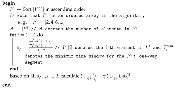
The first strategy is the ”Earliest Arrival” strategy (EAS), in which the ship captain determines the average speed of travel based on the earliest time window for the next one-way segment. The second strategy is the ”Latest Arrival” strategy (LAS), in which the ship captain determines the average speed of travel based on the latest time window for the next one-way segment. The third strategy is the ”Median Arrival” strategy (MAS). We assume that the ship captain prefers to arrive in the middle of the time window and, therefore, determines the average speed of travel based on the median of the time window for the next one-way segment.
The detailed algorithms for realizing these three benchmark strategies are shown in Algorithm 1, Algorithm 2 and Algorithm 3.
| Algorithm 1: EAS |
![Mathematics 11 04747 i001]() |
| Algorithm 2: LAS |
![Mathematics 11 04747 i002]() |
| Algorithm 3: MAS |
![Mathematics 11 04747 i003]() |
6. Experiments
6.1. Experiment Settings
We have opted for an inland waterway route within the Yangtze River system (from Yibin to Shanghai) (
https://cjhy.mot.gov.cn/, accessed on 30 August 2023) to test the performance of Model [M2]. The details are shown in
Table 2.
For the parameter settings, we first set the values of the parameters to draw the basic results, and we conducted sensitivity analysis to examine the impacts of these parameters. Referring to [
37], we first set
per week for a 300-TEU (twenty-foot equivalent unit) container ship. Additionally, referring to [
38], we set
to be an average value of 600 (
$/tonne). According to previous research, we set
[
36]. Moreover, the departure time
was set to 7:00, and the port of discharge was set within the time window
(the latest arrival time is day 6 20:00).
The experiments were run on a laptop computer equipped with 2.60 GHz of Intel Core i7 CPU and 16 GB of RAM, and Model [M2] was solved by the Gurobi Optimizer 10.0.2 via the Python API.
6.2. Basic Results
Using the route in
Table 2, we conducted numerical experiments, and we report the results in
Table 3. As defined in
Section 3, the entire inland waterway consists of two-way segments at the beginning and end with alternating one-way and two-way channels. The optimal value of the objective function of model [M2] is represented by “OBJ”.
Based on the results in
Table 3, in general, the solution model represents a multistage decision-making process, wherein the shipping company determines the optimal sailing speed for each segment based on the distances and time window ranges of the one-way channels [
39]. Additionally, the company selects a suitable time window for entering each one-way segment to ensure vessel arrival at the port of discharge within the designated time window
, thereby facilitating its unloading operations.
Specifically, in segment 1, the vessel maintained a high speed, since the company decided to enter segment 2 within the time window of , and the ship needed to reach segment 2 no later than 19:00. For segments 2 and 3, the vessel sailed at speeds of 13.99 knots and 15.58 knots, respectively. Considering the relatively longer total distances of segments 2 and 3, the company chose to enter segment 4 within the time window of to ensure timely access with a sailing speed 11.73 knots. Taking into account the requirement of reaching the destination port within the time window of and considering the accumulated time consumed by the previous four segments, the vessel still had ample time for navigation. Hence, in segments 5, 6, and 7, the vessel adopted relatively slower sailing speeds of 11.75, 8.48, and 8.48 knots, respectively. The entry into segment 6 was planned within the time window of . On the whole, the total cost of the entire inland waterway amounted to . The entire decision-making process took into comprehensive consideration various factors such as the distance of each segment and the time windows of the one-way channels, thereby aiming to achieve the overall optimization of the decisions.
6.3. Comparison with Three Basic Strategies
For the EAS strategy, we deduced the sailing speeds of each segment by considering the earliest time windows and the arrival times at the port of discharge, in addition to the speed constraints of each leg. For instance, when calculating the sailing speed of segment 1, the nearest time window came out to be
. Thus, the optimal sailing speed could be obtained as
. Consequently, the optimal sailing speed would be set to 16. By following this approach, we were able to derive the sailing speeds for each leg. By referring to
Table 4, we observe that the sailing speeds for each leg were significantly higher compared to the values provided in
Table 3. Hence, the vessel arrived at the port of discharge within the earliest time window. Nevertheless, such speed enhancements entail an increase in fuel consumption, thus leading to a rise in fuel costs. After performing the calculations, the total cost for the EAS strategy amounted to
, thus exceeding the total cost obtained through our optimization model.
Similar to the calculation method employed in the preceding EAS strategy, the LAS strategy also relied on considering the earliest time windows, the arrival times at the port of discharge, and the sailing speed constraints for each one-way segment to deduce the respective sailing speeds. For instance, when calculating the sailing speed for segment 1, we encountered the nearest time window, which is denoted as
. Consequently, the optimal sailing speed was determined as
. Thus, the ideal streaming speed was set to 8.17. Using this approach, the sailing speeds for each subsequent segment could be determined accordingly. Upon examining
Table 5, we notably observe that the sailing speeds for each segment were significantly lower compared to the prescribed values provided in
Table 3. However, due to the LAS strategy’s selection of the latest time windows for entry, this resulted in prolonged waiting periods upon entering segment 4 and segment 6. Specifically, delays of 12 h and 52 min and 14 h and 37 min were encountered, respectively. Consequently, significant time was lost, thereby preventing the vessel from reaching the port of discharge within the stipulated time window.
Similar to the aforementioned approach, in the MAS strategy, we integrated various factors such as segment distances, streaming speed constraints, and the medians of the time windows to deduce the sailing speeds for each segment. For instance, when calculating the sailing speed for segment 1, the nearest time window was
, and the median of this time window was 16. Consequently, the optimal sailing speed was denoted as
. Hence, the optimal sailing speed for segment 1 should be set at 10.89 knots. Following this methodology, the sailing speeds for each subsequent segment could be computed accordingly. By referring to
Table 6, we discern that certain route segments exhibited sailing speeds that aligned with the sailing speed trends observed in
Table 3. Furthermore, the vessel arrives at the port of discharge during the median of the time window (136.5), which was slightly earlier than the arrival times in
Table 3. However, it is worth noting that the MAS strategy incurred a total cost of
, which surpasses the total cost calculated using our optimization model.
Through comparison, we have observed that our research model demonstrates the capacity to effectively integrate various factors such as segment distances, time windows, and velocity constraints. It enables the optimal determination of sailing speeds and time windows for each segment, thereby ensuring timely arrival at the port of discharge while minimizing the overall costs to the greatest extent possible. This aptly showcases the efficacy of our model, as it adeptly combines these elements to achieve optimal outcomes. The costs under three different strategies are displayed in
Figure 2.
7. Discussion
From a theoretical standpoint, our research is centered on the intricate optimization of vessel speed and the precise timing of entry into various types of waterway routes within the realm of inland waterway transportation. By meticulously integrating time windows and the classification of waterway types into our mathematical model, we have made a significant and nuanced contribution to the existing body of research surrounding decision-making processes in inland waterway transportation.
From a practical perspective, our research offers a multifaceted array of substantial advantages. On the one hand, we have conducted a meticulous examination of time window constraints within single-lane waterway channels to derive the optimal sailing speeds for vessels. This, in turn, guarantees their prompt arrival while concurrently substantially reducing fuel consumption. The profound implications of this optimization are twofold. Firstly, it streamlines operational logistics for shipping companies, thereby leading to substantial cost reductions. Additionally, it has a direct and positive impact on fuel efficiency, thus resulting in a tangible reduction in carbon emissions associated with inland water transportation. This dual effect aligns with the broader goals of environmental sustainability and green practices, thereby advocating for a more ecoconscious approach in the industry.
Furthermore, our research extends its practical applicability by offering insights into the identification of the optimal time windows for vessels navigating single-lane segments. This invaluable knowledge assists vessels in navigating through specific waterways with pinpoint accuracy, thus avoiding extended waiting periods brought about by missed entry windows. This strategic approach not only diminishes vessel idle times, but also contributes significantly to the reduction in carbon emissions during these otherwise unproductive phases. In essence, our research serves as a dual force for both operational efficiency and environmental sustainability within the domain of inland water transportation, thus championing the reduction of carbon emissions and the promotion of green, sustainable practices in the industry.
8. Conclusions
By integrating the current state of inland waterways transportation with the backdrop of green and sustainable development, this study created an IP model for routes that involve alternating between single and dual navigational channels. The model determines the optimal speed for each route segment and identifies the best time windows for entering a single-direction channel, thereby ensuring that ships arrive at the port of discharge within the specified time while minimizing costs. Additionally, the IP model developed in this study was compared against three benchmark strategies (the EAS, LAS, and MAS) to showcase its clear advantages. In summary, our research has far-reaching managerial implications for the inland waterway transportation industry. Beyond its theoretical and practical contributions, it provides valuable insights that can guide decision makers within shipping companies and help shape the future of inland waterway transportation management from these aspects: (i) Cost reduction: One of the most significant managerial implications of our research is in cost reduction. Shipping companies can utilize our model to optimize vessel speeds and entry times, thereby reducing operational costs. By minimizing fuel consumption and voyage durations, these companies can enhance their cost-efficiency, thus resulting in substantial savings. (ii) Operational efficiency: The research equips shipping companies with tools to make informed decisions about vessel operations. It streamlines logistics by ensuring timely port arrivals and reducing waiting times. This increased operational efficiency can lead to better resource allocation and overall improved performance. (iii) Risk mitigation: The model can help mitigate operational risks. By identifying optimal entry times into single-lane segments, companies can avoid costly delays and disruptions, which can be crucial in maintaining service reliability and customer satisfaction. (iv) Environmental responsibility: Our research aligns with the growing trend towards environmental responsibility and sustainability. Shipping companies can leverage the insights from this research to reduce carbon emissions by minimizing fuel consumption and idle times. Generally, our research is not just a theoretical exercise, but also offers tangible benefits and strategic advantages for shipping companies. By integrating the principles and findings of this study into their operations, companies can improve their cost-efficiency, operational effectiveness, environmental responsibility, and competitive standing in the market.
Additionally, our study does bear certain limitations. In the development of our model, our primary focus centered on two pivotal factors: vessel speed and time window constraints. Regrettably, in the course of designing our model, we regrettably did not account for the interplay between cargo weight and fuel consumption, as well as the impact of weather conditions and river water levels. This omission has, to a certain extent, impeded the model’s broader applicability. In particular, for the relationship between cargo weight and fuel consumption, while our model construction and comprehensive review of the literature revealed an empirically substantiated cubic correlation between vessel speed and fuel consumption, a notable gap persists in quantifying the nuanced interplay between cargo weight and fuel consumption. Considering the acknowledged limitations of our study, several avenues for further research can be delineated to enhance the comprehensiveness and practical relevance of the modeling approach in the realm of inland waterway transportation optimization: (i) Integration of Additional Variables: Future research endeavors should prioritize the integration of crucial variables that have hitherto been omitted. Most notably, factors such as cargo weight, weather conditions, and other pertinent environmental elements should be incorporated into the model’s framework. The inclusion of these variables would undoubtedly lead to a more comprehensive and sophisticated understanding of the multifaceted dynamics that influence vessel speed optimization and the determination of optimal entry time windows. Cargo weight, for instance, plays a pivotal role in fuel consumption and vessel performance. Weather conditions, including wind speed, precipitation, and temperature, can significantly impact navigation and fuel efficiency. By considering these variables, the model can attain a higher degree of accuracy and real-world relevance, thereby enhancing its practical applicability in the field of inland waterway transportation. (ii) Dynamic Modeling and Real-Time Data: A paramount avenue for future research lies in the development of dynamic models that possess the capability to adapt to real-time data. This represents a substantial leap forward in terms of decision-making precision and responsiveness. By harnessing real-time information concerning variables such as weather patterns, traffic congestion, water levels, and other dynamic factors, the model can make on-the-fly adjustments, thus ensuring that decisions are based on the most up-to-date and accurate data available. The incorporation of real-time data transforms the model into a dynamic and versatile tool that can significantly enhance its practicality. This real-time adaptability is particularly crucial in a constantly evolving environment like inland waterway transportation, where conditions can change rapidly. (iii) Simulation and Scenario Analysis: To comprehensively assess the model’s efficacy and robustness, it is imperative to embark on extensive simulation studies and scenario analyses. These analyses constitute a vital step toward evaluating how the model performs under various conditions and scenarios. By subjecting the model to a spectrum of simulated situations, researchers can gain profound insights into its sensitivity to different parameters and its capacity to adapt to diverse operational contexts. These studies are instrumental in identifying potential weaknesses, limitations, and areas for improvement. They also serve as a foundation for refining the model’s underlying algorithms and logic, thereby ultimately enhancing its predictive power and decision-making accuracy. Consequently, the model’s reliability and real-world utility would be significantly bolstered, thus offering a more valuable tool for decision makers in the inland waterway transportation industry. By venturing into these suggested research pathways, our research can progress towards a more all-encompassing and actionable comprehension for optimizing inland waterway transportation. Ultimately, this will contribute to elevated sustainability, efficiency, and well-informed decision making within the industry.
In general, this investigation makes a significant contribution to understanding the strategies of inland shipping companies operating in routes that involve alternating between single and dual navigational channels. Overall, our study offers valuable insights into how informed decisions can be made, thereby considering the specific characteristics of such routes. By providing efficient solution methods and comparing them with three benchmark strategies, our research provides practical guidance for optimal speed decisions and time window decisions in shipping routes.


