Article

Output Feedback Control Design for Switched Systems with Unmatched Uncertainties Based on the Switched Robust Integral Sliding Mode

1
Beijing Key Laboratory of Robot Bionics and Function Research, Beijing University of Civil Engineering and Architecture, Beijing 100044, China
2
Key Laboratory of AI and Information Processing, Education Department of Guangxi Zhuang Autonomous Region, Hechi University, Hechi 546300, China
*
Author to whom correspondence should be addressed.
Mathematics 2023, 11(22), 4674; https://doi.org/10.3390/math11224674
Submission received: 12 September 2023 / Revised: 26 October 2023 / Accepted: 14 November 2023 / Published: 16 November 2023

Abstract

:
This paper proposes an output feedback sliding-mode control design based on a switched robust integral sliding mode for switched systems with unmatched uncertainties. First, the control task based on the observer is given while the system state information cannot be measured directly. Then, the switched robust integral sliding mode is constructed on the space of the estimated state, while the parameters of the switched robust integral sliding mode are selected ensuring that the system state in the sliding mode is robustly and exponentially stable. Linear matrix inequality conditions for the stabilization switching rule and the common Lyapunov function criterion are achieved. Consequently, the corresponding sliding-mode controller is designed based on the state estimation and the switched robust integral sliding mode. Finally, the application simulation results in a one-link manipulator with the load change validate the effectiveness and feasibility.

1. Introduction

Switched systems are very attractive in the research of hybrid system or complex system theory and application. A switched system (SS) is generally composed of a group of continuous or discrete dynamic subsystems and a certain switching rule that switches each subsystem. Many control methods of switched systems have been applied to many practical engineering systems, such as chemical processes, transportation transmission processes, computer control systems, and power systems. Simultaneously, switched systems have received widespread attention from scholars in the past few decades [1,2,3].
The control system state is sometimes not directly measurable. In practice, the varying parameters, the sampling of the state and input–output signals, and the disturbance or exogenous perturbations are all issues that the control system has to confront. Some research works on these problems were presented. For example, Tóth et al. discussed the discretization issue for linear parameter-varying (LPV) state-space systems in terms of the approximation error considering the actual sampling of the input–output signals [4]. Krasnova et al. presented the block approach to design the tracking control for a nonlinear system while the output variables are interfered by the exogenous perturbations [5]. Andrievsky and Furtat proposed a comprehensive discussion of the disturbance observation methods and their applications [6,7]. Simultaneously, for switched systems, it is necessary to study how to achieve feedback stabilization or trajectory tracking without state feedback information. At this point, the complexity of control design and switching strategy design increases. Therefore, the control problem of switched systems based on output feedback or observers has become one of the main research topics in the field of switched systems [8,9,10,11]. For example, Li et al. studied the observer-based stabilization of linear switched systems [12]. El Farra et al. designed an output feedback controller for input-constrained nonlinear switching systems using the multiple Lyapunov function method, and designed a switching strategy based on state observations [13]. Zhang et al. addressed the issue of fixed-time sliding-mode output tracking control for second-order switched systems [14]. Qi et al. investigated the adaptive output feedback control problem for nonlinear uncertain switched systems with input quantization, unmeasured system states, and state constraints [15].
In recent years, output feedback sliding-mode control (SMC) for uncertain switched systems has achieved many beneficial results [16,17,18], because SMC has strong robustness against matched uncertainties/perturbations [19,20]. The robust observation technique based on the SMC methodology is well-suited to resolve the output feedback control issue of uncertain SSs due to its ability to counteract external disturbances and model uncertainties [21], which were shown in some recent research work. For example, Gao et al. presented a reduced-order observer-based sliding-mode control scheme for switched descriptor systems to guarantee the exponentially asymptotic stability of the sliding motions [22]. Kchaou et al. investigated an asynchronous adaptive observer so as to stabilize a class of nonlinear stochastic switched systems with Markovian switching signals [23]. Some fixed-time or finite-time observers were proposed. Qi et al. studied the sliding-mode control for semi-Markov switching systems with quantized measurement and gave the corresponding finite-time observer design [24]. Likewise, Zhang et al. designed a nonfragile finite-time bounded sliding-mode observer for stochastic Markovian jump systems with a deterministic switching chain [25]. Also, a similar observer-based SMC for “fuzzy stochastic” switched systems under cyber attacks was investigated in [26]. Some scholars focused on fault diagnosis and isolation problems by using the sliding-mode observers. Li et al. presented a robust fault diagnosis for switched systems based on sliding-mode observers and applied it to a DC–DC power electronic converter [27]. Zhang et al. proposed a fault detection and isolation (FDI) method [28]. On the other hand, Meng et al. dealt with the problem of observer-based event-triggered sliding-mode control for fractional-order uncertain switched systems [29].
The integral sliding mode (ISM) method [30,31] is the well-known way to eliminate the reaching phase of the SMC control methodology. The system can reach onto the ISM surface from the initial time instant, and the overall robustness of the sliding mode is obtained. Moreover, it can be easy to form a second-order sliding mode and the high-order SMC after the modification of the sliding-mode surface [32]. The ISM method has been successfully applied to uncertain SSs, in order to suppress the matched uncertainties or perturbations. For example, Kchaou and Al Ahmadi extended an adaptive SMC design based on the ISM for a class of uncertain switched descriptor systems with state delay and nonlinear input [33]. Chen et al. investigated a robust exponential stabilization H -based integral sliding-mode controller design for uncertain stochastic Takagi–Sugeno (T-S) fuzzy switched time-delay systems [34]. Qi et al. studied the issue of sliding-mode control design for a class of nonlinear semi-Markovian switching systems via the T-S fuzzy approach by designing an ISM surface [35]. Zhang presented a robust integral sliding-mode control under arbitrary time-dependent switching rules for uncertain switched systems [36]. However, these studies did not consider the situation of immeasurable state information. Some scholars considered the output feedback control design or observer-based SMC via the ISM method for switched systems. Kao et al. concerned a non-fragile observer-based integral sliding-mode control for a class of uncertain switched hyperbolic systems [37]. Wang et al. presented a sliding-mode dynamic output feedback controller design based on the ISM for Markovian jump systems [38].
However, these output feedback control designs based on the ISM method for uncertain SSs cannot deal with unmatched uncertainty and disturbance. Inspired by the ISM method, this paper presents a robust integral sliding mode (RISM) design for switched systems with unmatched uncertainties. First, the control task is described as a general output feedback stabilization based on the observer. Additionally, an RISM designed on an estimated state space is presented, whose parameters can guarantee an exponentially stable sliding motion with robustness to the unmatched uncertainties. Every subsystem can reject structured unmatched uncertainties. Then, linear matrix inequality conditions for the RISM parameters and the switching rule are achieved. Afterwards, the SMC controller is designed and the corresponding stability of the RISM is analyzed. The main contribution of this paper is to provide an output feedback SMC control design based on the switched robust integral sliding mode (SRISM) scheme for uncertain SSs with unmatched uncertainties, in which the sliding motion is still robust to unmatched uncertainty or disturbance.
The remainder of the paper is organized as follows. The problem formulation is described in Section 2. The definition of the SRISM sliding surface and the design of the sliding-mode parameters are given in Section 3, and the stability in the sliding mode is analyzed. Then, the reachability of the sliding mode is proven in Section 4 after the SMC controller design. Application simulation results are presented in Section 5. Finally, the conclusion is given in Section 6.

2. Problem Formulation

Consider the following uncertain switched system:
x ˙ ( t ) = ( A σ + Δ A σ ) x ( t ) + ( B σ + Δ B σ ) u ( t ) + G σ ω σ ( t ) y ( t ) = C σ x ( t ) ,
where x t R n is the system state vector; u t R m is the control input; y ( t ) R p is the system output; Δ A σ , Δ B σ represent the uncertainties of the parameter matrices A σ , B σ , respectively; ω σ ( t ) denotes the bounded exogenous disturbance; and σ : R N 1 , 2 , , N presents the piecewise constant function σ ( t ) , i.e., the function of time t, which is also referred to as the switching signal (rule). Then, we define a switching sequence:
Q : = x t 0 ; i 0 , t 0 , i 1 , t 1 , , i k , t k , , i k N , k Z +
where x t 0 is the state value at the initial time t 0 . Namely, the i k -th subsystem runs when t t k , t k + 1 .
For the switching signal σ t = i , i N , the i-th subsystem matrices are denoted as:
A σ A i , B σ B i , G σ G i , C σ C i , Δ A σ Δ A i , Δ B σ Δ B i , ω σ ( t ) ω i ( t ) .
Accordingly, for the k-th switching, when t k t < t k + 1 , we can set σ t = i , i.e., i k = i N . As a result, the system (1) can be described as:
x ˙ ( t ) = A i + Δ A i x t + B i + Δ B i u t + G i ω i t y t = C i x t .
To ensure the control synthesis, the controllability and observability of the nominal subsystem are to be satisfied, and the uncertainties and disturbance are to be bounded [39]. Namely, the following assumptions are satisfied and the lemmas described below are used in this work.
Assumption 1.
( A i , B i ) is stabilizable and B i is required to be a full column rank; ( A i . C i ) is observable.
Assumption 2.
The uncertainty parameters, Δ A i and Δ B i , satisfy the following relationships:
Δ A i = H a , i F a , i t E a , i , Δ B i = H b , i F b , i t E b , i ,
where H a , i R n × r a , H b , i R n × r b , E a , i R r a × n and E b , i R r b × m are all of the known-constant matrices, and the unknown time-varying matrices F a , i t R r a × r a and F b , i t R r b × r b satisfy:
F a , i T t F a , i t I , F b , i T t F b , i t I .
Assumption 3.
The bounded disturbance ω i ( t ) satisfies ω i ( t ) < d i , in which d i is a positive scalar parameter.
Lemma 1.
Assuming that H and E are the matrices consisting of real constants with appropriate dimensions, F ( t ) satisfies F T t F t I . The following relation is true for any positive constant ε > 0 [40]:
H F t E + E T F T t H T ε 1 H H T + ε E T E .
When the system state x ( t ) cannot be measured directly, the following state observer is constructed:
x ^ ˙ t = A i x ^ t + B i u t + L i y t C i x ^ t ,
where x ^ ( t ) is the observation of the system state x ( t ) , and L i R n × p is the designed observer feedback gain, which can make the matrices
A ¯ i = A i L i C i , i N
to be Hurwitz.
Defining the state observation error as x ˜ t = x t x ^ t . By (3), (6) and (7), we obtain:
x ˜ ˙ t = A ¯ i + Δ A i x ˜ t + Δ A i x ^ t + Δ B i u t + G i ω i t .
The control task is to design an SMC control for guaranteeing the asymptotic stability of the switched system as described by (1), (3) with the unmatched uncertainties to realize the robust output feedback stabilization based on the state observer (6).
Remark 1.
The uncertainties and disturbance in the SS (3) include the matched, which occurs at the control input channel, and the unmatched, which cannot be treated in the common sliding-mode designs. They are essentially described as the time-varying Δ A i ( t ) , Δ B i ( t ) , G i ω i ( t ) , and can be decomposed as (4). They cover a wide range of structured uncertainties and disturbances.

3. Switched Robust Integral Sliding-Mode Surface Design via the State Observer

3.1. Sliding Surface with Multiple Sliding Modes

We present the following definition of the sliding surface with multiple sliding modes for the SS (1) [41].
Definition 1.
The hypersurface
S x , t : = S σ ( t ) ( x , t ) = 0 | σ ( t ) f o l l o w s Q , σ ( t ) N
is a sliding surface with multiple sliding modes of the SS (1) that consists of the sliding modes S i ( x , t ) , i N of the subsystems, and
S i x , t = 0 , w h e n σ ( t ) = i
along with the switching rule σ ( t ) (2). Namely, it is a type of switched sliding mode (SSM).
Remark 2.
The continuity of the sliding surface with multiple sliding modes plays a crucial role, namely the state x ( t k ) will be on the next sub-sliding mode S i ( x ( t k ) , t k ) = 0 when the switching occurs t = t k .
Remark 3.
The hypersurface (9) is composed of every sub-hyper plane S i ( x , t ) = 0 with every switching σ ( t ) = i that at the switching time t = t k must have the interface between every two switching instances, namely σ ( t ) = i 1 and i.
The diagrammatic sketch of the switched sliding surface and the SSM is shown as Figure 1. (The lines in different colors represent the different running subsystems).

3.2. Sliding Mode Design of Subsystems

We design a RISM based on the observer (6) as:
S ^ i x ^ , t = D i x ^ t x ^ t k + t k t ( K i D i A i ) x ^ t d t
in which the parameter D i R m × n satisfies
i N , rank ( D i B i ) = m , and 0 γ i < 1 , γ i R , D i Δ B i γ i D i B i ;
another parameter K i is the common-state-feedback stabilization coefficient to be designed and it essentially ensures that the matrices
A ^ i = A i B i ( D i B i ) 1 K i , i N
are Hurwitz.
Based on (6) and (10), we can write:
S ^ ˙ i x ^ , t = K i x ^ t + D i B i u t + D i L i y t C i x ^ t .
According to the sliding-mode control theory, when the system state reaches the sliding surface and remains there, S ^ i ( x ^ , t ) = 0 , S ^ ˙ i ( x ^ , t ) = 0 . Thus, the equivalent control can be written as:
u e q t = D i B i 1 K i x ^ t + D i L i y t C i x ^ t .
By substituting (13) into (6) and using (12), the sliding-mode equation can be written as:
x ^ ˙ t = A ^ i x ^ t + H y , i y t C i x ^ t , H y , i = L i B i ( D i B i ) 1 D i L i .

3.3. SRISM Sliding-Mode Surface and Its Stability

The robust integral sliding mode (10) of every subsystem (3) has been designed based on the observer (6) and the corresponding sliding-mode dynamic (14) is obtained. All of the sliding-mode dynamics S ^ i x ^ , t = 0 comprise the sliding surface with multiple sliding modes S ^ i ( x ^ , t ) = 0 , i follows Q .
However, the whole switched system (3) under the switching signal σ ( t ) (the switching sequence Q) is not ensured to be robustly stable. It can be assumed that the observer state x ^ ( t ) runs onto the corresponding RISM surface and remains there when the switching σ ( t ) = i occurs at time t k . This property can be easily ensured because S ^ i ( x ^ ( t k ) , t k ) = 0 by (10). Consequently, it is important to keep the observer state x ^ ( t ) on the RISM surface at all times, which is carried out by the sliding-mode controller. If we consider that this is achieved, the sliding surface with multiple sliding modes for the SS (1) is obtained as (9) according to Definition 1.
This sliding-mode surface S ^ i ( x ^ , t ) = 0 , i follows Q can also be called the SRISM because its component S i ( x , t ) = 0 is the RISM. Now, we can state that the system state x is running on the sliding surface or the SRISM { S ^ i ( x ^ , t ) = 0 } . Namely, the switched system (3) is under its sliding mode.
When the switched system (3) is running under the sliding mode, its stability depends on dynamic (14). There are two typical approaches for guaranteeing the stability of SRISM based on the stability analysis. One is the common Lyapunov function (CLF) method, and the other is the multiple Lyapunov-like functions (MLF) method. Additionally, the robust stability depends on the sliding-mode parameters D i , K i .
The design criterion of the parameters D i and K i for the RISM (10) is presented as follows.
Theorem 1.
Given positive scalars α i > 0 for the switched system (1), if i N , there exist the matrices P i > 0 , Q > 0 and any positive scalars ε 1 , i , ε 2 , i , ε 3 , i , ε i > 0 that satisfy
Θ 1 , i 0 P i H y , i 0 0 0 0 Θ 2 , i 0 Q H a , i Q H b , i Q G i ε 1 , i I 0 0 0 0.5 ε 2 , i I 0 0 0.5 ε 3 , i I 0 ε i I < 0 ,
where:
Θ 1 , i = P i A ^ i + A ^ i T P i + α i P i + ε 2 , i E a , i T E a , i + ε 3 , i E ¯ b , i T E ¯ b , i , Θ 2 , i = Q A ¯ i + A ¯ i T Q + α i Q + ε 1 , i C i T C i + ε 2 , i E a , i T E a , i + ε 3 , i E ˜ b , i T E ˜ b , i , E ¯ b , i = E b , i D i B i 1 K i , E ˜ b , i = E b , i ( D i B i ) 1 D i L i C i ;
then, the system state running on the sliding-mode surface { S ^ i x ^ , t = 0 } will be stable by the control of the switching rule
σ ( t 0 ) = argmin i N x ^ T t 0 P i x ^ t 0
σ t k = i , x ^ t k Λ i and σ t k 1 = i , argmin i N x ^ T t P i P j x ^ t , x ^ t k Λ i and σ t k 1 = j , j i
Λ i = x ^ ( t ) | x ^ T ( t ) ( P i P j ) x ^ ( t ) 0 , j N , j i .
Furthermore, the closed-loop system satisfies the following:
(1) 
When ω i ( t ) 0 , the system state will be exponentially stable.
(2) 
When ω i ( t ) 0 , the system state trajectory will exponentially converge to
lim t x t max i N ε i d i 2 α i λ min ( P i ) + ε i d i 2 α i λ min ( Q )
Proof. 
Selecting the Lyapunov function as
V i t = x ^ T t P i x ^ t + x ˜ T t Q x ˜ t
for the i-th subsystem and finding its derivative with respect to the time along with (8) and (14), one obtains:
V ˙ i ( t ) = x ^ T ( t ) ( P i A ^ i + A ^ i T P i ) x ^ ( t ) + 2 x ˜ T ( t ) Q [ ( A ¯ i + Δ A i ) x ˜ ( t ) + Δ A i x ^ ( t ) ] + 2 x ˜ T ( t ) Q [ Δ B i u t + G i ω i ( t ) ] + 2 x ^ T ( t ) P i H y , i ( y ( t ) C i x ^ ( t ) ) .
This is because the system reaches into the sliding mode S ^ i x ^ , t = 0 , S ^ ˙ i x ^ , t = 0 , and u ( t ) = u e q ( t ) . Substituting (13) into the above equation, one obtains:
V ˙ i ( t ) = x ^ T ( t ) ( P i A ^ i + A ^ i T P i ) x ^ ( t ) + 2 x ˜ T ( t ) Q [ ( A ¯ i + Δ A i ) x ˜ ( t ) + Δ A i x ^ ( t ) ] 2 x ˜ T ( t ) Q [ Δ B i ( D i B i ) 1 K i x ^ ( t ) + Δ B i ( D i B i ) 1 D i L i C i x ˜ ( t ) ] + 2 x ˜ T ( t ) Q G i ω i ( t ) + 2 x ^ T ( t ) P i H y , i C i x ˜ ( t ) .
Based on Assumption 2 and Lemma 1, for any positive scalars ε 1 , i , ε 2 , i , ε 3 , i , ε i , the following inequalities can be obtained:
2 x ^ T t P i H y , i C i x ˜ ( t ) ε 1 , i 1 x ^ T t P i H y , i H y , i T P i x ^ ( t ) + ε 1 , i x ˜ T t C i T C i x ˜ ( t ) , 2 x ˜ T t Q Δ A i x ˜ t ε 2 , i 1 x ˜ T t H a , i Q H a , i T x ˜ t + ε 2 , i x ˜ T t E a , i T E a , i x ˜ t , 2 x ˜ T t Q Δ A i x ^ t ε 2 , i 1 x ˜ T t Q H a , i Q H a , i T x ˜ t + ε 2 , i x ^ T t E a , i T E a , i x ^ t , 2 x ˜ T t Q Δ B i ( D i B i ) 1 D i L i C i x ˜ t ε 3 , i 1 x ˜ T t Q H b , i Q H b , i T x ˜ t + ε 3 , i x ˜ T t E ˜ b , i T E ˜ b , i x ˜ t , 2 x ˜ T t Q Δ B i D i B i 1 K i x ^ t ε 3 , i 1 x ˜ T t Q H b , i Q H b , i T x ˜ t + ε 3 , i x ^ T t E ¯ b , i T E ¯ b , i x ^ t , 2 x ˜ ( t ) T Q G i ω i ( t ) ε i 1 x ˜ T t Q G i ( Q G i ) T x ˜ ( t ) + ε i ω i T ( t ) ω i ( t ) .
From (21) and (22), it can be deduced that
V ˙ i t ζ T t W i ζ t + ε i ω i T t ω i t ,
where:
ζ t = x ^ T t x ˜ T t T , W i = diag Σ i , 1 , Σ i , 2 , Σ i , 1 = P i A ^ i + A ^ i T P i + ε 1 , i 1 P i H u , i H u , i T P i + ε 2 , i E a , i T E a , i + ε 3 , i E ¯ b , i T E ¯ b , i , Σ i , 2 = Q A ¯ i + A ¯ i T Q + 2 ε 2 , i 1 Q H a , i H a , i T Q + 2 ε 3 , i 1 Q H b , i H b , i T Q + ε i 1 Q G i G i T Q + ε 1 , i C i T C i + ε 2 , i E a , i T E a , i + ε 3 , i E ˜ b , i T E ˜ b , i .
Then, by (23) and (24), the following inequality holds:
V ˙ i t + α i V i t ε i ω i T t ω i t ζ T t W i + α i diag P i , Q ζ t .
By the Schur Lemma, W i + α i diag P i , Q < 0 is equivalent to the LMI (15). Consequently, the following inequality holds:
V ˙ i t + α i V i t ε i ω i T t ω i t 0 .
Two cases are to be discussed for the system stability.
(1)
In the case where ω i ( t ) 0 :
The inequality V ˙ i t + α i V i t 0 holds. Therefore, the trajectories of x ^ ( t ) and the observation error x ˜ ( t ) of the subsystem are exponentially stable. The subsystem state of the switched system (3) is hence exponentially stable.
(2)
In the case where ω i ( t ) 0 :
By Assumption 3, the Lyapunov function V i t satisfies the inequality
V i t V i t k e α i ( t t k ) + ε i d i 2 α i ,
which implies that the trajectories of x ^ ( t ) and the observation error x ˜ ( t ) satisfy
x ^ t 2 λ min 1 P i V i 0 e α i ( t t k ) + ε i d i 2 α i λ min P i , x ˜ t 2 λ min 1 Q V i 0 e α i ( t t k ) + ε i d i 2 α i λ min Q ,
namely,
lim t x ^ t ε i d i 2 α i λ min P i , lim t x ˜ t ε i d i 2 α i λ min Q .
Therefore, the subsystem state will exponentially converge to a small neighborhood of the origin.
From the switching rule (16)–(18), at the switching time point t k , the Lyapunov function of the corresponding subsystem is non-increasing. The following is true:
V i ( t k ) V j ( t k ) .
According to the MLF theory, the overall system state converges to the origin exponentially when ω i ( t ) 0 , or satisfies (19) when ω i ( t ) 0 . □
Remark 4.
The RISM (10) comprises the SRISM sliding-mode surface { S ^ i ( x ^ , t ) = 0 } for the SS (3). The condition (11) of the parameter D i is to guarantee that the uncertainty Δ B i does not affect its controllability. The SRISM is based on the state observer (6) and the conditions of Theorem 1 make the SRISM robust to the unmatched uncertainty.
Based on Theorem 1, the following corollaries can be achieved.
Corollary 1.
For the switched system (1), if i N , there exist the matrices P i > 0 , Q > 0 and the positive scalars ε 1 , i , ε 2 , i , ε 3 , i , ε i > 0 that satisfy
Θ ¯ 1 , i 0 P i H y , i 0 0 0 0 Θ ¯ 2 , i 0 Q H a , i Q H b , i Q G i ε 1 , i I 0 0 0 0.5 ε 2 , i I 0 0 0.5 ε 3 , i I 0 ε i I < 0 ,
where:
Θ ¯ 1 , i = P i A ^ i + A ^ i T P i + I + ε 2 , i E a , i T E a , i + ε 3 , i E ¯ b , i T E ¯ b , i , Θ ¯ 2 , i = Q A ¯ i + A ¯ i T Q + I + ε 1 , i C i T C i + ε 2 , i E a , i T E a , i + ε 3 , i E ˜ b , i T E ˜ b , i ;
then, the system state running on the sliding-mode surface { S ^ i ( x ^ , t ) = 0 } will be stable under the switching rule (16)–(18). Furthermore, the closed-loop system satisfies the following:
(1) 
When ω i ( t ) 0 , the system state will be asymptotically stable, i.e., lim t x t = 0 .
(2) 
When ω i ( t ) 0 , the following inequality
t 0 x T τ x τ d τ γ t 0 max ω i T τ ω i τ d τ .
holds under the initial condition of zero, where γ = max ε i is the L2 performance index.
Proof. 
Selecting the Lyapunov function as (20) and finding its time derivative, one obtains the relationship (23), (24) according to the proof of Theorem 1. Consequently, the following inequality holds:
V ˙ i t + x T t x t γ ω i T t ω i t V ˙ i t + ζ T t ζ t γ ω i T t ω i t ζ T t W i + I ζ t + ( ε i γ ) ω i T t ω i t .
By the Schur Lemma, W i + I < 0 is equivalent to the LMI (25). Obviously, if the condition (25) holds, one can obtain the following inequality:
V ˙ i t + x T t x t γ ω i T t ω i t < 0 .
Additionally, a similar analysis to the proof of Theorem 1 can be conducted. Two cases are to be discussed for the system stability.
(1)
In the case where ω i ( t ) 0 :
The inequality V ˙ i t x T t x ( t ) holds. Therefore, the trajectories of x ^ ( t ) and the observation error x ˜ ( t ) of the subsystem are asymptotically stable. The subsystem state of the switched system (3) is hence asymptotically stable. Furthermore, by the switching rule (16)–(18), at the switching time point t k , the Lyapunov function of the corresponding subsystem is non-increasing, and V i ( t k ) V j ( t k ) holds. According to the MLF theory, the overall system state converges to the origin asymptotically when ω i ( t ) 0 .
(2)
In the case where ω i ( t ) 0 :
The inequality
t k t x T τ x τ d τ V i t k V i ( t ) + γ t k t ω i T τ ω i τ d τ
holds for every subsystem. At the time interval t [ t 0 , t ] with t k < t t k + 1 , the following inequality holds:
t 0 t x T τ x τ d τ V i 0 ( t 0 ) V i 0 ( t 1 ) + V i 1 ( t 1 ) V i 1 ( t 2 ) + + V i k ( t k ) V i k ( t k + 1 ) + γ t 0 t max { ω i T τ ω i τ } d τ .
According to the switching rule (16)–(18), V i ( t k ) V j ( t k ) . Therefore, the inequality
t 0 x T τ x τ d τ V i 0 ( t 0 ) V i k ( ) + γ t 0 max { ω i T τ ω i τ } d τ
holds along with t . If the initial condition of the system state is zero, V i 0 ( t 0 ) = 0 , amd the inequality (26) holds obviously. □
Corollary 2.
Given positive scalars α i > 0 for the switched system (1), if i N , there exist the matrices P > 0 , Q > 0 and any positive scalars ε 1 , i , ε 2 , i , ε 3 , i , ε i > 0 that satisfy
Θ 1 , i 0 P H y , i 0 0 0 0 Θ 2 , i 0 Q H a , i Q H b , i Q G i ε 1 , i I 0 0 0 0.5 ε 2 , i I 0 0 0.5 ε 3 , i I 0 ε i I < 0 ,
where:
Θ 1 , i = P A ^ i + A ^ i T P + α i P + ε 2 , i E a , i T E a , i + ε 3 , i E ¯ b , i T E ¯ b , i , Θ 2 , i = Q A ¯ i + A ¯ i T Q + α i Q + ε 1 , i C i T C i + ε 2 , i E a , i T E a , i + ε 3 , i E ˜ b , i T E ˜ b , i ;
then, the system state running on the sliding-mode { S ^ i x ^ , t = 0 } will be stable under arbitrary switching rules. Furthermore, the closed-loop system satisfies the following:
(1)
When ω i ( t ) 0 , the system state will be exponentially stable.
(2)
When ω i ( t ) 0 , the system state trajectory will exponentially converge to
lim t x t max i N ε i d i 2 α i λ min ( P ) + ε i d i 2 α i λ min ( Q ) .
Proof. 
Selecting the CLF as
V t = x ^ T t P x ^ t + x ˜ T t Q x ˜ t
for the SS (3) and finding its derivative with respect to the time along with (8) and (14), one easily obtains
V ˙ t + α i V t ε i ω i T t ω i t 0
according to the proof of Theorem 1. Therefore, a similar conclusions will be achieved. □

4. SMC Controller

We design the output feedback SMC controller based on the observer (6) as
u ( t ) = u 0 ( t ) + u 1 ( t ) , u 0 t = D i B i 1 K i x ^ t + D i L i y t C i x ^ t , u 1 t = D i B i 1 η i S ^ i x ^ , t + ρ i sgn S ^ i x ^ , t ,
where the parameters are designed as η i > 0 , ρ i > 0 .
The SMC controller (31) is composed of two parts: the output feedback equivalent control part u 0 and the discontinuous part u 1 .
Theorem 2.
For the switched system (3) with the state observer (6), the observation state trajectory will be kept on the sliding-mode surface { S ^ i x , t = 0 } from the initial time instant and be retained there keeping the movement on the sliding mode under the SMC control (31).
Proof. 
Selecting the Lyapunov function as
V ( t ) = i = 1 N λ i S ^ i T ( x ^ , t ) S ^ i ( x ^ , t ) ,
where λ i > 0 , i N are positive scalars, according to (10), the time derivative of V ( t ) is:
V ˙ ( t ) = i = 1 N λ i S ^ i T x ^ , t [ K i x ^ t + D i B i u ( t ) + D i L i y t C i x ^ t ] } .
Substituting the SMC controller (31) into the above equation, one obtains
V ˙ t = i = 1 N λ i S ^ i T x ^ , t η i S ^ i x ^ , t i = 1 N λ i S ^ i T x ^ , t ρ i sgn S ^ i x ^ , t .
This means that the observer state x ^ ( t ) will converge to the sliding-mode surface S ^ i ( x ^ , t ) = 0 within the limited time. From the RISM (10), S ^ i ( x ^ , t k ) = 0 is easily satisfied only if the initial observation state x ^ ( t k ) is known. Therefore, the observation state retains there, keeping the movement on the sliding-mode surface from the initial time instant. □
Remark 5.
Theorem 2 shows that the sliding-mode controller (31) makes every RISM of the subsystem reachable from the initial time t k , when the switching occurs. Therefore, all of the S ^ i ( x ^ , t ) = 0 following the switching sequence Q will comprise the sliding surface with multiple sliding modes defined in Definition 1.

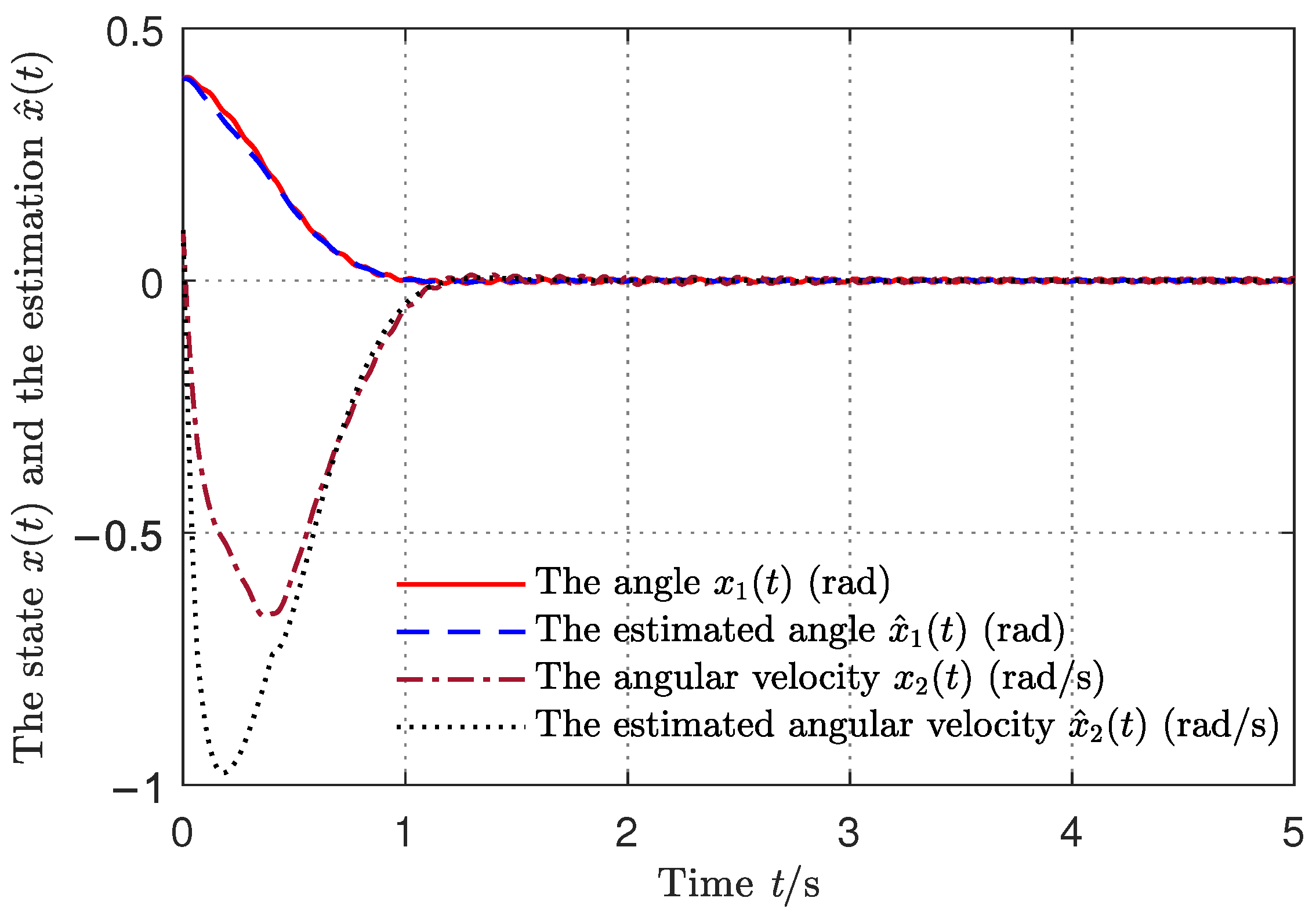
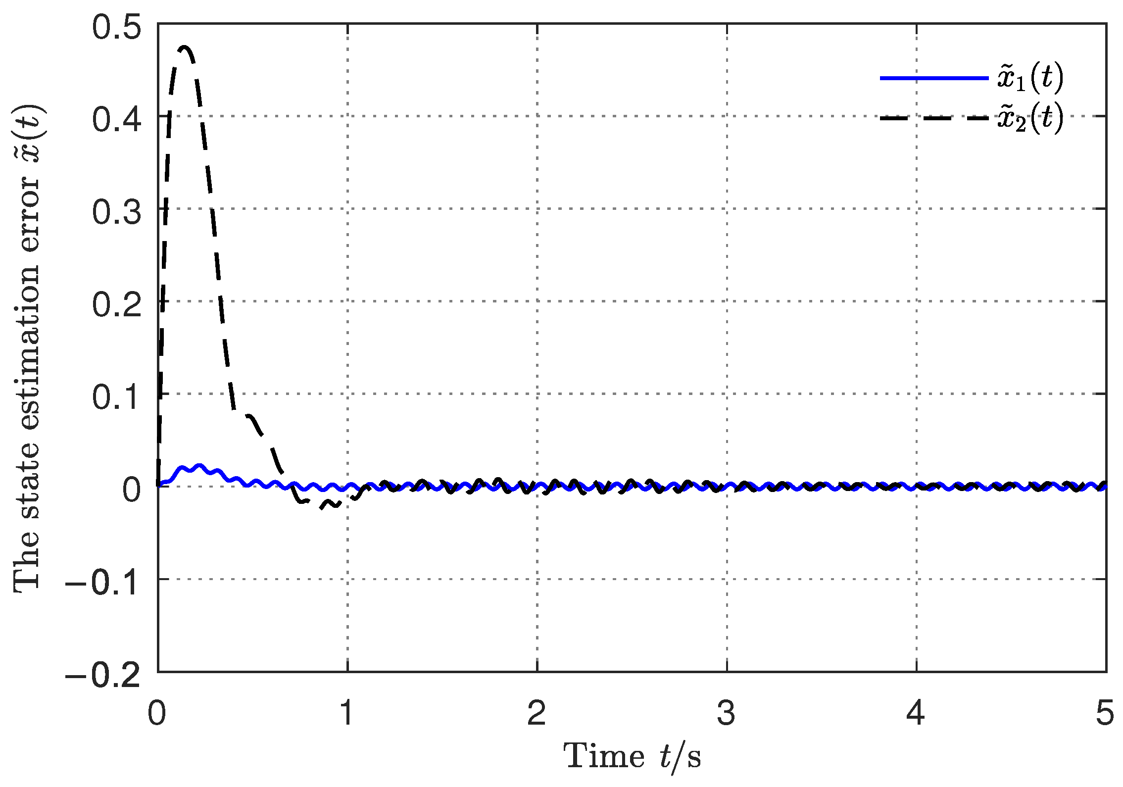
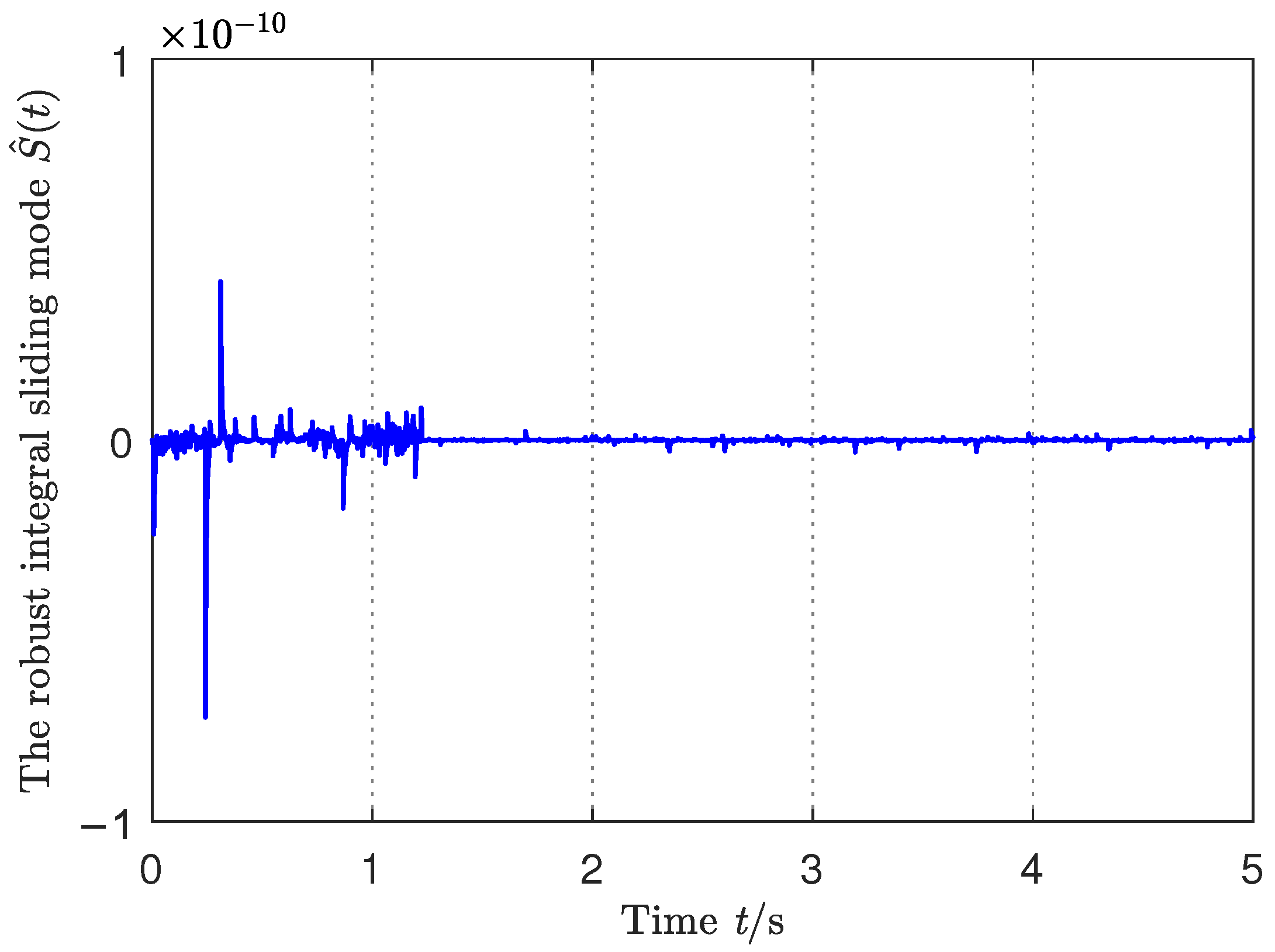
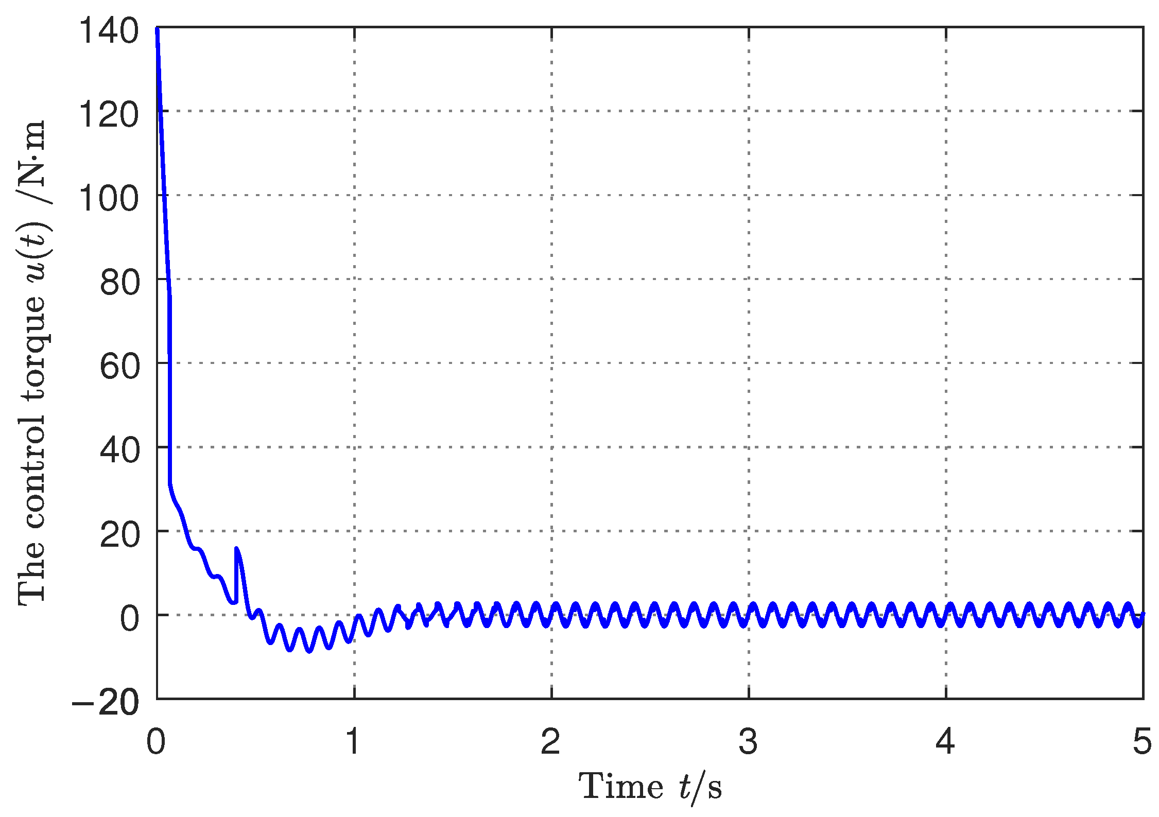
5. Illustrative Example

Consider a one-link robotic manipulator whose joint angle can only be acquired directly. Its mathematical description is as follows:
x ˙ 1 ( t ) = x 2 ( t ) + ϕ 1 ( t ) , x ˙ 2 ( t ) = m g l m l 2 + J cos x 1 ( t ) + 1 m l 2 + J u ( t ) + ϕ 2 ( t ) , y ( t ) = x 1 ( t ) ,
where x 1 ( t ) is the joint angle, x 2 ( t ) is the angular velocity, x ( t ) = [ x 1 ( t ) , x 2 ( t ) ] T is the state vector, m is the mass of the beam, l is the beam length, g represents the gravitational acceleration, and J is the moment of inertia. The control torque is u ( t ) and ϕ 1 ( t ) , ϕ 2 ( t ) indicate the exogenous disturbances. It is considered that z 1 ( t ) = 0.5 π x 1 ( t ) , i.e., z 1 ( t ) is the complementary angle of the joint angle with z 2 ( t ) = z ˙ 1 ( t ) = x 2 ( t ) ; and only the angle z 1 ( t ) can be measured. In this way, by applying the approximation sin z 1 ( t ) z 1 ( t ) , the mathematical model (34) is transformed into the linear form
z ˙ ( t ) = ( A + Δ A ) z ( t ) + B u ( t ) + G w ( t ) , y ( t ) = C z ( t ) ,
where z ( t ) = [ z 1 ( t ) , z 2 ( t ) ] T is the transformed state vector, and w ( t ) = [ ϕ 1 ( t ) , ϕ 2 ( t ) ] T denotes the exogenous disturbance. The parameter matrices are as follows:
A = 0 1 m g l m l 2   +   J 0 , Δ A = 0 1 Δ m g l cos Δ z 1 m l 2   +   J 0 , B = 0 1 m l 2   +   J T , G = I , C = 1 0 T .
When the manipulator grasps different parts in industrial operations, the physical parameters m , l , and J will change along with its operation conditions. Therefore, two cases with different loads lead to the switched system with two sets of parameters of the system (35):
A 1 = 0 1 m 1 g l 1 m 1 l 1 2   +   J 1 0 , A 2 = 0 1 m 2 g l 2 m 2 l 2 2   +   J 2 0 , B 1 = 0 1 m 1 l 1 2   +   J 1 , B 2 = 0 1 m 2 l 2 2   +   J 2 , Δ A 1 = 0 0 Δ m g l 1 cos Δ z 1 m 1 l 1 2   +   J 1 0 , Δ A 2 = 0 0 Δ m g l 2 cos Δ z 1 m 2 l 2 2   +   J 2 0 , Δ B 1 = 0 1 m 1 l 1 2   +   Δ J T , Δ B 2 = 0 1 m 2 l 2 2   +   Δ J T ,
where Δ m represents the mass changes when the load of the manipulator varies, i.e., Δ m = ± | m 1 m 2 . Similarly, Δ J represents the inertia changes, i.e., Δ J = ± | J 1 J 2 | . The physical parameters are given as m 1 = 3 kg , m 2 = 4 kg , l 1 = 1 m , l 2 = 1.2 m , J 1 = 0.5 kg · m 2 , J 2 = 0.6 kg · m 2 . It can be proven that i N , ( A i , B i ) can be stabilizable and ( A i , C i ) is observable. According to Assumption 2, the uncertainties are decomposed as the following matrices:
H a , 1 = 0 14 , H a , 2 = 0 9.25 , F a , 1 = F a , 2 = cos Δ z 1 , E a , 1 = E a , 2 = 0.2 0 , H b , 1 = 0 6 T , H b , 2 = 0 2 T , F b , 1 = F b , 2 = 1 , E b , 1 = E b , 2 = 0.01 .
According to the parameter design conditions (11), the parameters D 1 = [ 1 5 ] , D 2 = [ 0 5 ] are selected. It can be verified that i N , D i B i is of full rank. Moreover, the parameter design conditions (12) are verified. To select the matrices L 1 = [ 22 , 104.4 ] T , L 2 = [ 24 , 135.4 ] T , and K 1 = [ 225 , 60 ] , K 2 = [ 260 , 60 ] , by (7) and (12) we have:
A ¯ 1 = 22 1 96 0 , A ¯ 2 = 24 1 128 0 , A ^ 1 = 0 1 45 12.2 , A ^ 2 = 0 1 52 12 ,
whose eigenvalues are all negative.
After the above-described calculations, it can be verified whether D and K can make a RISM based on Theorem 1. Given the positive scalars α 1 = α 2 = 0.5 , we can directly solve the LMIs (15) using the LMI toolbox in Matlab. The matrices P 1 , P 2 , and Q are found to be:
P 1 = 88.69 19.82 19.82 5.55 , P 2 = 80.41 16.55 16.55 4.39 , Q = 241.57 12.1 12.1 3.35 ,
and the RISM (10) is obtained.
We set the system state initial value as z ( t 0 ) = [ 0.4 , 0.1 ] T . The sliding-mode controller under the designed switching rules (16)–(18) can be used by Theorem 1, for which ρ i = 2 and η i = 10 are set. By substituting D i , K i , A i , B i , and C i into (31), the practical output feedback switched controller can be obtained. When the unmatched exogenous perturbation ϕ 1 ( t ) = 0.2 cos 20 π t and the matched ϕ 2 ( t ) = 0.1 sin 20 π t , the stabilization of the one-link manipulator was validated as shown in Figure 2, Figure 3, Figure 4, Figure 5 and Figure 6.
In Figure 2, the estimation of the angular velocity x ^ 2 ( t ) is with a slightly larger deviation during the transient. This is dependent on the observer dynamic (6). The transient performance can be improved by changing its placed poles, but the robustness must be taken care of by Theorem 1. Figure 2, Figure 3 and Figure 4 display the state running results of the switched system. From these figures we can observe that under the existence of uncertain parameters and perturbations, the system state remains on the sliding surface with the designed switching rule from the initial time onward. The control torque signal is shown in Figure 5 and the corresponding switching signal is shown in Figure 6 by the switching rule in Theorem 1. The switching signal shows that the switching action was impacted by the cycle disturbances ϕ 1 ( t ) and ϕ 2 ( t ) especially at the steady state. This is because the state variables have been disturbed by the exogenous perturbations and the switching rule is dependent on the calculation of (16)–(18).

6. Conclusions

A switched robust integral sliding mode designed on the estimated state space of the observer for uncertain switched systems with unmatched uncertainties is presented. The proposed SRISM surface forms a robust stable sliding motion, which has the ability to suppress the unmatched uncertainties. The design conditions of the SRISM parameters are given as linear matrix inequities. The stability of the switched system in accordance with the proposed SRISM is ensured by two standard approaches. The first is the common Lyapunov function method, and the second is stabilization via the switching rule. The stability criteria for the system in the sliding mode are given. The simulation results of the application to a one-link manipulator are proposed to illustrate the output feedback control design. The effectiveness and the feasibility of the proposed design are validated.
The robust SMC control design for uncertain SSs with unmatched uncertainties and disturbances still has some issues to be investigated. The dwell-time-based SMC control design based on the proposed SRISM, in which the dwell time of every subsystem will be focused and the Zeno phenomenon, will be considered. How to form the second-order or high-order sliding mode by using the proposed SRISM is another consideration. These issues will potentially be examined in the future to obtain the better performance.

Author Contributions

Conceptualization, X.Z.; methodology, X.Z.; validation, X.Z. and S.X.; formal analysis, X.Z. and S.X.; writing—original draft preparation, X.Z.; writing—review and editing, X.Z. and S.X. All authors have read and agreed to the submitted version of the manuscript.

Funding

This work was supported financially by the Open Project Fund of the Key Laboratory of AI and Information Processing (2022GXZDSY005), the National Natural Science Foundation of China (62371032), and the Cultivation Project Funds for Beijing University of Civil Engineering and Architecture (X23049).

Institutional Review Board Statement

Not applicable.

Informed Consent Statement

Not applicable.

Data Availability Statement

No new data were created or analyzed in this study. Data sharing is not applicable to this article.

Acknowledgments

The authors would like to thank the editors and the reviewers for their work.

Conflicts of Interest

The authors declare no conflict of interest.

References

  1. Liberzon, D. Switching in Systems and Control; Birkhauser: Boston, MA, USA, 2003. [Google Scholar]
  2. Margaliot, M. Stability analysis of switched systems using variational principles: An introduction. Automatica 2006, 42, 2059–2077. [Google Scholar] [CrossRef]
  3. Wu, L.; Shi, P.; Su, X. Sliding Mode Control of Uncertain Parameter-Switching Hybrid Systems; John Wiley & Sons: Hoboken, NJ, USA, 2014. [Google Scholar]
  4. Tóth, R.; Felici, F.; Heuberger, P.; Van den Hof, P. Crucial aspects of zero-order hold LPV state-space system discretization. IFAC Proc. Vol. 2008, 41, 4952–4957. [Google Scholar] [CrossRef]
  5. Krasnova, S.A.; Utkin, V.A.; Utkin, A.V. Block approach to analysis and design of the invariant nonlinear tracking systems. Autom. Remote Control 2017, 78, 2120–2140. [Google Scholar] [CrossRef]
  6. Andrievsky, B.R.; Furtat, I.B. Disturbance observers: Methods and applications. I. Methods. Autom. Remote Control 2020, 81, 1563–1610. [Google Scholar] [CrossRef]
  7. Andrievsky, B.R.; Furtat, I.B. Disturbance observers: Methods and applications. II. Applications. Autom. Remote Control 2020, 81, 1775–1818. [Google Scholar] [CrossRef]
  8. Wang, J.; Huo, S.; Xia, J.; Park, J.H.; Huang, X.; Shen, H. Generalised dissipative asynchronous output feedback control for Markov jump repeated scalar nonlinear systems with time-varying delay. IET Control Theory Appl. 2019, 13, 2114–2121. [Google Scholar] [CrossRef]
  9. Geromel, J.C.; Colaneri, P.; Bolzern, P. Dynamic Output Feedback Control of Switched Linear Systems. IEEE Trans. Autom. Control 2008, 53, 720–733. [Google Scholar] [CrossRef]
  10. Li, L.; Zhao, J.; Dimirovski, G.M. Observer-based reliable exponential stabilization and control for switched systems with faulty actuators: An average dwell time approach. Nonlinear Anal. Hybrid Syst. 2011, 5, 479–491. [Google Scholar] [CrossRef]
  11. Deaecto, G.S.; Geromel, J.C.; Daafouz, J. Dynamic output feedback control of switched systems. Automatica 2011, 47, 1713–1720. [Google Scholar] [CrossRef]
  12. Li, Z.G.; Wen, C.Y.; Soh, Y.C. Observer-based stabilization of switching linear systems. Automatica 2005, 41, 181–195. [Google Scholar] [CrossRef]
  13. El-Farra, N.H.; Mhaskar, P.; Christofides, P.D. Output feedback control of switched nonlinear systems using multiple Lyapunov functions. Syst. Control Lett. 2005, 54, 1163–1182. [Google Scholar] [CrossRef]
  14. Zhang, Y.; Sun, H.; Sun, C. Fixed-time sliding mode output tracking control for second-order switched systems with power integrators. Comput. Electr. Eng. 2021, 96, 107503. [Google Scholar] [CrossRef]
  15. Qi, S.; Zhao, J.; Tang, L. Adaptive Output Feedback Control for Constrained Switched Systems with Input Quantization. Mathematics 2023, 11, 788. [Google Scholar] [CrossRef]
  16. Qi, Y.; Hu, J. Observer-based bumpless switching control for switched linear systems with sensor faults. Trans. Inst. Meas. Control 2018, 40, 1490–1498. [Google Scholar] [CrossRef]
  17. Zhao, H.; Niu, Y.; Song, J. Finite-time output feedback control of uncertain switched systems via sliding mode design. Int. J. Syst. Sci. 2018, 49, 984–996. [Google Scholar] [CrossRef]
  18. Yin, S.; Gao, H.; Qiu, J.; Kaynak, O. Descriptor reduced-order sliding mode observers design for switched systems with sensor and actuator faults. Automatica 2017, 76, 282–292. [Google Scholar] [CrossRef]
  19. Wu, L.; Lam, J. Sliding mode control of switched hybrid systems with time-varying delay. Int. J. Adapt. Control Signal Process. 2008, 22, 909–931. [Google Scholar] [CrossRef]
  20. Wu, L.; Ho, D.W.C.; Li, C.W. Sliding mode control of switched hybrid systems with stochastic perturbation. Syst. Control Lett. 2011, 60, 531–539. [Google Scholar] [CrossRef]
  21. Shtessel, Y.; Edwards, C.; Fridman, L.; Levant, A. Sliding Mode Control and Observation; Birkhauser, Springer: New York, NY, USA, 2014. [Google Scholar]
  22. Gao, R.; Zhai, D.; Xie, X. On the design of output information-based sliding mode controllers for switched descriptor systems: Linear sliding variable approach. Appl. Math. Comput. 2020, 364, 124680. [Google Scholar] [CrossRef]
  23. Kchaou, M.; Regaieg, M.A.; Al-Hajjaji, A. Quantized asynchronous extended dissipative observer-based sliding mode control for Markovian jump TS fuzzy systems. J. Frankl. Inst. 2022, 359, 9636–9665. [Google Scholar] [CrossRef]
  24. Qi, W.; Zong, G.; Karimi, H.R. Finite-time observer-based sliding mode control for quantized semi-Markov switching systems with application. IEEE Trans. Ind. Inform. 2020, 16, 1259–1271. [Google Scholar] [CrossRef]
  25. Zhang, P.; Kao, Y.; Hu, J.; Niu, B.; Xia, H.; Wang, C. Finite-time observer-based sliding-mode control for Markovian jump systems with switching chain: Average dwell-time method. IEEE Trans. Cybern. 2023, 53, 248–261. [Google Scholar] [CrossRef] [PubMed]
  26. Zhang, N.; Qi, W.; Pang, G.; Cheng, J.; Shi, K. Observer-based sliding mode control for fuzzy stochastic switching systems with deception attacks. Appl. Math. Comput. 2022, 427, 127153. [Google Scholar] [CrossRef]
  27. Li, J.; Guo, X.; Chen, C.; Su, Q. Robust fault diagnosis for switched systems based on sliding mode observer. Appl. Math. Comput. 2019, 341, 193–203. [Google Scholar] [CrossRef]
  28. Zhang, Z.H.; Li, S.; Yan, H.; Fan, Q.Y. Sliding mode switching observer-based actuator fault detection and isolation for a class of uncertain systems. Nonlinear Anal. Hybrid Syst. 2019, 33, 322–335. [Google Scholar] [CrossRef]
  29. Meng, X.; Jiang, B.; Karimi, H.R.; Gao, C. An event-triggered mechanism to observer-based sliding mode control of fractional-order uncertain switched systems. ISA Trans. 2023, 135, 115–129. [Google Scholar] [CrossRef]
  30. Utkin, V.I.; Shi, J. Integral sliding mode in systems operating under uncertainty conditions. In Proceedings of the 35th IEEE Conference on Decision and Control, Kobe, Japan, 13 December 1996; pp. 4591–4596. [Google Scholar]
  31. Cao, W.J.; Xu, J.X. Nonlinear integral-type sliding surface for both matched and unmatched uncertain systems. IEEE Trans. Autom. Control 2004, 49, 1355–1360. [Google Scholar] [CrossRef]
  32. Pan, Y.; Yang, C.; Pan, L.; Yu, H. Integral sliding mode control: Performance, modification, and improvement. IEEE Trans. Ind. Inform. 2018, 14, 3087–3096. [Google Scholar] [CrossRef]
  33. Kchaou, M.; Al Ahmadi, S. Robust H control for nonlinear uncertain switched descriptor systems with time delay and nonlinear input: A sliding mode approach. Complexity 2017, 2017, 1027909. [Google Scholar] [CrossRef]
  34. Chen, H.; Lim, C.C.; Shi, P. Robust H-based control for uncertain stochastic fuzzy switched time-delay systems via integral sliding mode strategy. IEEE Trans. Fuzzy Syst. 2022, 30, 382–396. [Google Scholar] [CrossRef]
  35. Qi, W.; Gao, X.; Ahn, C.K.; Cao, J.; Cheng, J. Fuzzy integral sliding-mode control for nonlinear semi-Markovian switching systems with application. IEEE Trans. Syst. Man Cybern. Syst. 2022, 52, 1674–1683. [Google Scholar] [CrossRef]
  36. Zhang, X. Robust integral sliding mode control for uncertain switched systems under arbitrary switching rules. Nonlinear Anal. Hybrid Syst. 2020, 37, 100900. [Google Scholar] [CrossRef]
  37. Kao, Y.; Liu, X.; Song, M.; Zhao, L.; Zhang, Q. Nonfragile-observer-based integral sliding mode control for a class of uncertain switched hyperbolic systems. IEEE Trans. Autom. Control 2023, 68, 5059–5066. [Google Scholar] [CrossRef]
  38. Wang, C.; Li, R.; Su, X.; Shi, P. Output feedback sliding mode control of Markovian jump systems and its application to switched boost converter. IEEE Trans. Circuits Syst. I Regul. Pap. 2021, 68, 5134–5144. [Google Scholar] [CrossRef]
  39. Lian, J.; Ge, Y. Robust H output tracking control for switched systems under asynchronous switching. Nonlinear Anal. Hybrid Syst. 2013, 8, 57–68. [Google Scholar] [CrossRef]
  40. Wang, Y.; Xie, L.; Souza, C.E.D. Robust control of a class of uncertain nonlinear systems. Syst. Control Lett. 1992, 19, 139–149. [Google Scholar] [CrossRef]
  41. Zhang, X.; Xiao, L.; Li, H. Robust control for switched systems with unmatched uncertainties based on switched robust integral sliding mode. IEEE Access 2020, 8, 138396–138405. [Google Scholar] [CrossRef]
Figure 1. Sketch of the sliding surface and the SSM.
Mathematics 11 04674 g001
Figure 2. The angle and angular velocity and their estimation curves.
Mathematics 11 04674 g002
Figure 3. The observation error curves of the state variables.
Mathematics 11 04674 g003
Figure 4. The RISM signal curve under the sliding mode.
Mathematics 11 04674 g004
Figure 5. The control torque curve with the proposed control design.
Mathematics 11 04674 g005
Figure 6. The switching signal by the switching rule (16)–(18).
Mathematics 11 04674 g006
Disclaimer/Publisher’s Note: The statements, opinions and data contained in all publications are solely those of the individual author(s) and contributor(s) and not of MDPI and/or the editor(s). MDPI and/or the editor(s) disclaim responsibility for any injury to people or property resulting from any ideas, methods, instructions or products referred to in the content.

