A Combined Runs Rules Scheme for Monitoring General Inflated Poisson Processes

Abstract

In this work, a control chart with multiple runs rules is proposed and studied in the case of monitoring inflated processes. Usually, Shewhart-type control charts for attributes do not have a lower control limit, especially when the in-control process mean level is very low, such as in the case of processes with a low number of defects per inspected unit. Therefore, it is not possible to detect a decrease in the process mean level. A common solution to this problem is to apply a runs rule on the lower side of the chart. Motivated by this approach, we suggest a Shewhart-type chart, supplemented with two runs rules; one is used for detecting decreases in process mean level, and the other is used for improving the chart’s sensitivity in the detection of small and moderate increasing shifts in the process mean level. Using the Markov chain method, we examine the performance of various schemes in terms of the average run length and the expected average run length. Two illustrative examples for the use of the proposed schemes in practice are also discussed. The numerical results show that the considered schemes can detect efficiently various shifts in process parameters in either direction.

1. Introduction

Statistical process monitoring (SPM) is a collection of methods and techniques which focus on the monitoring of a process and the timely detection of changes in it. The most frequently used SPM method is the control chart. The most common chart is the Shewhart chart, suggested by Walter A. Shewhart in the 1920’s, while there are two other main types of control charts, namely the cumulative sum (CUSUM) chart, proposed by Page [1], and the exponentially weighted moving average (EWMA) chart, proposed by Roberts [2]. A Shewhart chart is useful for the detection of sudden and of large magnitude shifts, while the CUSUM and EWMA charts are better than Shewhart charts in the detection of shifts of small magnitude. See [3] for more details on the properties and applications of the main types of control charts.

The superiority of CUSUM and EWMA charts in the detection of shifts of small magnitude is attributed to their inherent memory, i.e., the respective charting statistics consist of information not only from the most recent sample (or recent observation) but also from the past ones. However, even though their practical implementation is nowadays a routine application, there are still some difficulties in their statistical design, mainly in how to choose the most appropriate values for their chart parameters. From this point of view, intermediate solutions, such as supplementing a Shewhart chart with additional stopping rules based on runs (i.e., runs rules), are still popular in practical problems. We refer to [4,5] for thorough reviews of control charts with runs rules.

Control charts for attributes are used when count data are available from the process. This situation occurs when it is not possible to find a critical-to-quality (CTQ) characteristic $X$ (random variable, r.v.) that follows a continuous distribution. Usually, in the case of attributes charts, the distribution of $X$ can either take values on {0, 1, …} (e.g., in the case of monitoring the number of defects that follow a Poisson distribution) or on {0, 1, …, n} (e.g., in the case of monitoring the number of defective in a sample of size $n$, which follows a binomial distribution). Even though Poisson distribution and the associated Shewhart-type chart, the $c$-chart, are frequently used in the monitoring of count data, there are many cases where both are not appropriate. For example, this is the case of count data that exhibit over-dispersion, i.e., the variance of the distribution of $X$ is much larger than its mean. Recall that in Poisson distribution, mean and variance are equal. Therefore, a solution to this problem is to adopt a distributional model for the available count data from the process that can capture this deviation from the ordinary Poisson model.

Inflated probability distributions have been studied by several authors due to their flexibility in modeling over-dispersion in the data. A common sub-class of the family of inflated distributions is that of zero-inflated distributions (see, for example, Chapter 8 in [6]), where the probability for the occurrence of a zero value is much larger than the respective probability under the non-inflated distribution. Even though inflated distributions (not necessarily only at zero) have been studied in the past (Yoneda [7]), in recent years, there has also been interest in extending them to model the inflation of two or more values. See, for example, [8,9,10,11] and references therein for inflated distributions in exactly two values: at 0 and at another one non-zero value. Also, Sun et al. [12] suggested a zero-one-two inflated distribution, a distribution inflated at exactly three values. Begum et al. [13] and Rakitzis et al. [14] proposed a general inflated Poisson model that takes into account the inflation on the first $r+1$ values (i.e., the $\{0, 1, \dots , r\}$) of the distribution. Also, Rakitzis et al. [14] proposed and studied a two-parameter mixture model, namely the $r$-geometrically inflated Poisson ($GI{P}_r$) distribution, which can model the inflation not only on the zero-values but also on other values of the Poisson distribution, while it has only two parameters.

Control charts for inflated distributions have been studied quite extensively in the recent literature, especially those related to the monitoring of zero-inflated processes. See the overview provided in [15]. Even though in the literature exists almost every main type of chart for inflated distributions (such as Shewhart, CUSUM, and EWMA), there are very few control charts with supplementary runs rules for monitoring this type of process. Actually, the case of attributes control charts with supplementary runs rules has not been paid much attention compared to their variable counterparts. Supplementing a Shewhart chart with runs rules is an easy-to-apply solution for the problem of their insensitivity in detecting small to moderate shifts in process parameter(s). We should also mention that it is very common for attribute charts to have no lower control limit, especially in the case of high-quality processes, where the fraction of non-conforming items is very low. For example, the lower control limit of a $c$-chart with 3 sigma limits and an IC mean lower than 9 is negative. In this case, it is suggested to use only an upper control limit on the chart (see [16]). Nelson [17], Acosta-Mejia [18], Lucas et al. [19], and Chang and Gan [20] studied attributes control charts with no lower control limit, and instead, they applied a runs rule on the lower side of the chart to detect a decrease in the process mean level.

Usually, high-quality processes can be modeled according to a discrete inflated probability distribution. Motivated by the works in [19,20], we propose and study a control chart with multiple runs rules to monitor a $GI{P}_r$ process and detect increases as well as decreases in its mean level. The aim is to suggest a control chart for attributes that retains the simplicity of a Shewhart-type chart with runs rules while it has an improved performance compared to its competitors. To the best of our knowledge, in the literature, there are no two-sided control charts with multiple runs rules for monitoring a $GI{P}_r$ processes. Also, it is worth noting that even though the properties of the proposed scheme are investigated in the case of monitoring a $GI{P}_r$ process, after some straightforward but necessary modifications, it can be used for the monitoring of any other process which is modeled according to a discrete probability distribution. These are the main scopes and motivations of this work.

The structure of this work is as follows: In Section 2, we present the main properties of the $GI{P}_r$ distribution. In Section 3, we introduce the proposed scheme and present the measures for evaluating its performance. In Section 4, we present the findings of an extensive numerical study regarding the statistical design and the performance of the proposed chart. Practical guidelines for applying the chart in practice are given as well. In Section 5, we present two illustrative examples (using real data), which show how to implement the proposed charts in practice. Finally, in Section 6, the conclusions and main findings of this work are summarized, while topics for future research are also given.

2. The r-Geometrically Inflated Poisson Distribution

We start this section by presenting the basic properties of the $r$-geometrically inflated Poisson distribution. Further details can be found in Rakitzis et al. [14]. Let $X$ be a discrete random variable with support $\mathcal{S}=\{0, 1, 2, \dots \}$. If the probability mass function (pmf) of $X$ is

$$f_{GI{P}_r}\left(x|\varphi ,\lambda \right)=\frac{{\varphi }^{x+1}}{r+1}{\mathrm{I}}_{\left\{0,1,\dots ,r\right\}}\left(x\right)+\frac{1}{r+1}\left(r+1-g_0\left(r,\varphi \right)\right)\frac{e^{-\lambda }{\lambda }^x}{x!}, x\in \left\{0,1,\dots \right\},$$

(1)

then we say that $X$ follows the $r$-geometrically inflated Poisson distribution with parameters $\varphi \in (0,1)$ (the inflation parameter), $\lambda >0$ and $r\in \{0, 1, 2, \dots \}$ (i.e., $X~GI{P}_r(\varphi ,\lambda )$). Also, $g_0\left(x,\varphi \right)=\varphi (1-{\varphi }^{x+1})/(1-\varphi )$ satisfies the inequality $r+1-g_0\left(r,\varphi \right)>0$ for every $\varphi \in (0,1)$ (so as $f_{GI{P}_r}\left(x\right|\varphi ,\lambda )$ is a true pmf), while ${\mathrm{I}}_A\left(x\right)$ is the usual indicator function. For $r=0$, the $GI{P}_r(\varphi ,\lambda )$ distribution reduces to the ZIP distribution with parameters $\varphi$ and $\lambda$.

The cumulative distribution function (cdf) $F_{GI{P}_r}\left(x\right|\varphi ,\lambda )$ of the $GI{P}_r(\varphi ,\lambda )$ distribution is given by

$$F_{GI{P}_r}\left(x|\varphi ,\lambda \right)=\left\{\begin{array}{cc}0,& x<0\\ \frac{1}{r+1}\left(g_0\left(⌊x⌋,\varphi \right)+\left(r+1-g_0\left(r,\varphi \right)\right)F_P\left(x|\lambda \right)\right),& 0\le x\le r\\ \frac{1}{r+1}\left(g_0\left(r,\varphi \right)+\left(r+1-g_0\left(r,\varphi \right)\right)F_P\left(x|\lambda \right)\right),& x\ge r+1\end{array}\right.$$

(2)

The $⌊\dots ⌋$ represents the smallest integer contained in $⌊\dots ⌋$ and $F_P\left(x\right|\lambda )$ is the cdf of the Poisson distribution with parameter $\lambda$. In addition, the mean of the $GI{P}_r(\varphi ,\lambda )$ distribution equals

$${\mu }_{GI{P}_r}=E\left(X\right)=\frac{g_1\left(r,\varphi \right)+\left(r+1-g_0\left(r,\varphi \right)\right)\lambda }{r+1},$$

(3)

where, for $\varphi \in (0,1)$, it is $g_1\left(x,\varphi \right)=\left(\frac{x{\varphi }^{x+1}-\left(x+1\right){\varphi }^x+1}{{\left(1-\varphi \right)}^2}\right){\varphi }^2$.

For a given $r$ value, the parameters $\varphi$ and $\lambda$ can be estimated by using either the maximum likelihood estimation method or the method of moments; see [14] for further details on estimation methods for the parameters of the $GI{P}_r(\varphi ,\lambda )$ distribution. In the present work, we assume that process parameters are known, or that they have been estimated from a (sufficiently) large Phase I sample.

3. The Proposed Monitoring Scheme

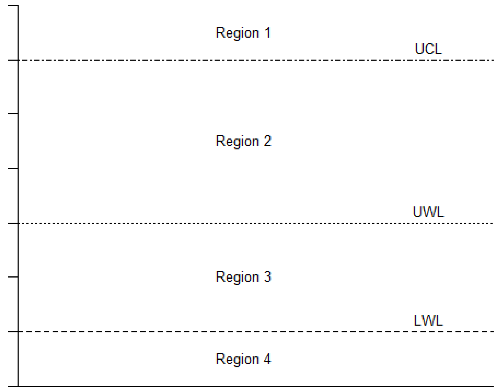
3.1. Operation of the Proposed Monitoring Scheme

In this section, we present the operation of the proposed monitoring scheme that can be used for the monitoring of a $GI{P}_r$ process. Following the setup in [21], we assume that the value of $r$ is predetermined and remains unaffected by the presence of assignable causes. Moreover, in this work the aim is to detect either upward or downward shifts in the in-control (IC) process mean level, which is denoted as ${\mu }_{0,GI{P}_r}$. The control charts studied by [21,22] can detect only upward shifts in ${\mu }_{0,GI{P}_r}$. Let us also assume that at each sampling stage, an individual observation is obtained from the $GI{P}_r$ process. We denote as ${\lambda }_0$, ${\varphi }_0$ the IC values of the process parameters. When the process is OOC, we assume that the OOC values of the process parameters are ${\lambda }_1=\delta \cdot {\lambda }_0$ and ${\varphi }_1=\tau \cdot {\varphi }_0$ with $\delta >0$ and $\tau \in (0,1/{\varphi }_0]$. When $\left(\tau ,\delta \right)=(1,1)$ the process is IC.

Both ${\mu }_{0,GI{P}_r}$ and ${\mu }_{1,GI{P}_r}$ are obtained via Equation (3) for the respective IC and OOC values of $\varphi$ and $\lambda$. It is worth mentioning that in practice, it is of great importance to detect an increase in the mean of the process, that is, a change from ${\mu }_{0,GI{P}_r}$ to ${\mu }_{1,GI{P}_r}>{\mu }_{0,GI{P}_r}$, because it is related to process deterioration. For example, control chart operators are interested in detecting an increase in the expected number of nonconformities of the inspected units or an increase in the expected weekly number of confirmed new infections from a specific disease. In addition, in modern statistical process monitoring (see, for example, [23,24,25,26]), the case of decreases is considered very important because it is related to process improvement. In such cases, the interest is in detecting a decrease in the expected number of non-conformities in the inspected units, which can be considered an indication that the attempts for process improvement have been successful. Note also that this improvement can be attributed to the occurrence of assignable causes, such as the recruitment of well-trained personnel or the use of improved raw materials. Consequently, for continuous improvement, it becomes essential to consider the improvement case. In this work, we consider both OOC cases: ${\mu }_{1,GI{P}_r}>{\mu }_{0,GI{P}_r}$ or ${\mu }_{1,GI{P}_r}<{\mu }_{0,GI{P}_r}$.

Let $l,m,k$ be positive integers with $2\le l\le m$ and $k\ge 2$. Then, the proposed monitoring scheme, to be denoted as ${CRR}_{l,m}$, gives an OOC signal when at least one of the following events occurs:

i.

A single value $X_t$ is beyond an upper control limit $UCL$ (Region 1);

ii.

l-out-of-m successive values are in the interval $(UWL,UCL]$ (Region 2) with the intermediate $m-l$ values being in the interval $(LWL,UWL]$ (Region 3);

iii.

k successive values are in the interval $[0,LWL]$ (Region 4);

whichever of the (i)–(iii) occurs first.

The suggested scheme can be viewed as an extension of the schemes studied by [19,20]. Specifically, in the above-mentioned works, the rule for detecting a decreasing shift in ${\mu }_{0,GI{P}_r}$ is of the type $k$-out-of-$k$ successive zero values. For the detection of increasing shifts in ${\mu }_{1,GI{P}_r}$, Lucas et al. [19] applied only the rule of a single value $X_t$ above an upper control limit $UCL$ while Chang and Gan [20] applied a rule of type $l$-out-of-$m$ consecutive points above an $UCL$.

The regions of the ${CRR}_{l,m}$ chart are given in Figure 1. To apply the proposed control chart in practice, the values of $LWL$, $UWL$, $UCL$, and $k$ must be determined for the given integer values $l,m$ ($2\le l\le m$). This is carried out via an appropriate design procedure; the values $(LWL,UWL,UCL,k)$ are determined so the ${CRR}_{l,m}$ scheme has the desired IC performance, and it is sensitive enough in the detection of specific shifts in process parameters.

Figure 1. Regions of the ${CRR}_{l,m}$ control chart.

3.2. Performance of the Proposed Monitoring Scheme

The performance of a process monitoring scheme is evaluated by the run length ($RL$) distribution, which is defined as the number of points plotted on the chart until it gives for the first time an OOC signal.

The computation of the $RL$ properties of the ${CRR}_{l,m}$ scheme is feasible using the finite Markov chain embedding technique of Fu and Koutras [27] (see also [28,29] and references therein). Further details on the method can be found in the Appendix A. Using this method, it is possible to calculate the entire $RL$ distribution, as well as its expected value $E\left(RL\right)$, which is known as the average run length ($ARL$). The $ARL$ is the most common performance measure of a control chart.

Apart from the $ARL,$ there are other performance measures that can be viewed as measures of the overall performance of the chart. Specifically, the $ARL$ evaluates the performance of a chart at a specific shift $(\tau ,\delta )$ in process parameters ${\varphi }_0$ and ${\lambda }_0$, respectively. In practice, these shifts are rarely known, or practitioners may want to know how the chart performs for a range of shifts. For this reason, in this work, we use also the expected average run length ($\mathit{EARL}$), which is defined as (see, for example, [30,31])

$$EARL=\frac{1}{({\tau }_{max}-{\tau }_{min})({\delta }_{max}-{\delta }_{min})}\underset{{\tau }_{min}}{\overset{{\tau }_{max}}{\int }}\underset{{\delta }_{min}}{\overset{{\delta }_{max}}{\int }}ARL(\tau ,\delta )d\delta d\tau ,$$

where $[{\delta }_{min},{\delta }_{max }]$ and $[{\tau }_{min},{\tau }_{max }]$ are the intervals for the shifts $\delta$ and $\tau$ in ${\lambda }_0$ and ${\varphi }_0$, respectively. The chart with the minimum $EARL$ is the one with the best overall performance at the specific range of shifts.

4. Numerical Results

In this section, we present the results of a numerical study regarding the performance of the ${CRR}_{l,m}$ chart. Specifically, we consider the following specific values for $l$, $m$ (see Table 1):

Table 1. The ${CRR}_{l,m}$ schemes under study.

Scheme	1	2	3	4	5	6	7
l	2	2	2	2	3	4	5
m	2	3	4	5	4	5	5
Notation	${CRR}_{2,2}$	${CRR}_{2,3}$	${CRR}_{2,4}$	${CRR}_{2,5}$	${CRR}_{3,4}$	${CRR}_{4,5}$	${CRR}_{5,5}$

These values correspond to very well-known runs rules such as the 2-of-2, the 2-of-3, and the 4-of-5, to mention a few.

Next, in Table 2 we provide six indicative scenarios for different IC $GI{P}_r$ processes. Cases 5 and 6 correspond to a zero-inflated Poisson (ZIP) process. The IC process mean level is given in the third row of Table 2 and varies from 0.4 to 2.6250 for the different 6 scenarios. Thus, they can be considered cases of high-quality processes.

Table 2. Scenarios for the IC $GI{P}_r$ Processes.

Case	1	2	3	4	5	6
$(r,{\varphi }_0,{\lambda }_0)$	$(3,0.7,3)$	$(3,0.7,1.5)$	$(2,0.9,3)$	$(1,0.5,4)$	$(0,0.8,2)$	$(0,0.9,6)$
${\mu }_{0,GI{P}_r}$	2.1442	1.3091	1.3170	2.6250	0.4000	0.6000

For each IC scenario in Table 2, we determined the values of the design parameters $LWL$, $UWL$, $UCL,$ and $k$ for the seven schemes in Table 1 to have comparable IC performance. For illustrative purposes, we considered an IC $ARL$ approximately equal to 100. Any other value can be used depending on practitioners’ needs.

The design procedure is based on an extensive grid search on the possible positive integer values for $LWL$, $UWL$, $UCL,$ and $k$ which satisfy the following two constraints: (I) $0\le LWL<UWL<UCL\le 15$ and (II) $k\in \{7, 8, \dots , 50\}$. Then, any combination of $LWL$, $UWL$, $UCL,$ and $k$ that gives an IC $ARL$ approximately equal to the pre-specified $AR{L}_0=100$ value, i.e., in the interval $(98,102)$, is considered accepted.

Once all the possible combinations for $(LWL,UWL,UCL,k)$ that give the desired IC performance have been determined, we evaluated the OOC $ARL$ of the proposed charts for several pairs of shifts $(\tau ,\delta )$. The considered pairs are $\left(\tau ,\delta \right)\in \left\{0.6,0.8,1,1.1\right\}\times \{0.5,0.8,1,1.2,1.5\}$ while for $\left(\tau ,\delta \right)=\left(1,1\right),$ the process is IC.

In Table 3, Table 4, Table 5, Table 6, Table 7 and Table 8 we provide the best charts, i.e., the ones with the minimum OOC $ARL$ values, for various shifts in ${\varphi }_0$ and ${\lambda }_0$ when the IC $ARL$ is (approximately) equal to 100. The shifts are given in columns ‘$\tau$’ and ‘$\delta$’, while the OOC values ${\lambda }_1$ and ${\varphi }_1$ of the process parameters are given in the respective columns. The column ‘${\mu }_{1,GI{P}_r}$’ gives the OOC process mean level, while the column ‘${\mu }_{1,GI{P}_r}/{\mu }_{0,GI{P}_r}$’ gives the change in IC process mean level. Note that when $\frac{{\mu }_{1,GI{P}_r}}{{\mu }_{0,GI{P}_r}}<1$, there is a decrease in the process mean level, otherwise, there is an increase. Also, the results in Table 3, Table 4, Table 5, Table 6, Table 7 and Table 8 have been sorted according to the values of this column to discriminate the decreases from the increases.

Table 3. Best charts in terms of $ARL$, Case 1, $AR{L}_0\approx 100$.

$\mathit{\tau }$	$\mathit{\delta }$	${\mathit{\lambda }}_1$	${\mathit{\varphi }}_1$	${\mathit{\mu }}_{1,\mathit{G}\mathit{I}{\mathit{P}}_{\mathit{r}}}$	$\frac{{\mathit{\mu }}_{1,\mathit{G}\mathit{I}{\mathit{P}}_{\mathit{r}}}}{{\mathit{\mu }}_{0,\mathit{G}\mathit{I}{\mathit{P}}_{\mathit{r}}}}$	$\mathit{A}\mathit{R}{\mathit{L}}_1$	$\mathit{L}\mathit{W}\mathit{L}$	$\mathit{U}\mathit{W}\mathit{L}$	$\mathit{U}\mathit{C}\mathit{L}$	$\mathit{k}$	Scheme	SH $\mathit{U}\mathit{C}{\mathit{L}}_{\mathit{S}\mathit{H}}=7$	$\mathit{\eta }/\mathit{\eta }$ $\mathit{\eta }=3$	Combined $\mathit{U}\mathit{C}{\mathit{L}}_{\mathit{S}\mathit{H}}=7$$, \mathit{\eta }=4$
1	0.5	1.5	0.70	1.3092	0.61	18.72	3	6	10	14	${CRR}_{2,2}$		51.84	173.69
0.8	0.5	1.5	0.56	1.3096	0.61	19.07	2	3	15	8	${CRR}_{4,5}$		51.89	173.11
1.1	0.5	1.5	0.77	1.3260	0.62	17.73	3	6	10	14	${CRR}_{2,2}$		54.06	184.28
0.6	0.5	1.5	0.42	1.3414	0.63	19.63	2	3	15	8	${CRR}_{4,5}$		56.87	194.78
1.1	0.8	2.4	0.77	1.7376	0.81	34.07	3	6	10	14	${CRR}_{2,2}$		100.60	261.13
1	0.8	2.4	0.70	1.8102	0.84	42.90	3	6	10	14	${CRR}_{2,2}$		111.30	258.62
0.8	0.8	2.4	0.56	1.9514	0.91	63.42	3	6	10	14	${CRR}_{2,2}$		145.35	264.59
1.1	1	3	0.77	2.0119	0.94	65.00	3	6	10	14	${CRR}_{2,2}$		126.47	140.21
0.6	0.8	2.4	0.42	2.0835	0.97	85.58	3	6	10	14	${CRR}_{2,2}$		208.52	276.92
1	1	3	0.70	2.1442	1.00							150.89	149.31	125.37
1.1	1.2	3.6	0.77	2.2863	1.07	48.53	0	5	7	7	${CRR}_{2,4}$	71.03		64.58
0.8	1	3	0.56	2.3793	1.11	59.11	2	3	9	12	${CRR}_{3,4}$	117.80		107.85
1	1.2	3.6	0.70	2.4783	1.16	37.64	0	5	7	7	${CRR}_{2,4}$	58.34		54.94
0.6	1	3	0.42	2.5783	1.20	41.15	2	3	9	12	${CRR}_{3,4}$	101.87		97.99
1.1	1.5	4.5	0.77	2.6978	1.26	17.90	0	5	7	7	${CRR}_{2,4}$	25.26		24.50
0.8	1.2	3.6	0.56	2.8072	1.31	26.17	1	4	9	10	${CRR}_{2,2}$	45.55		44.44
1	1.5	4.5	0.70	2.9793	1.39	14.05	0	5	7	7	${CRR}_{2,4}$	20.74		20.37
0.6	1.2	3.6	0.42	3.0730	1.43	18.46	2	3	9	12	${CRR}_{3,4}$	39.39		39.03
0.8	1.5	4.5	0.56	3.4490	1.61	10.30	0	5	7	7	${CRR}_{2,4}$	16.20		16.09
0.6	1.5	4.5	0.42	3.8152	1.78	8.55	0	5	7	7	${CRR}_{2,4}$	14.01		13.98

Table 4. Best charts in terms of $ARL$, Case 2, $AR{L}_0\approx 100$.

$\mathit{\tau }$	$\mathit{\delta }$	${\mathit{\lambda }}_1$	${\mathit{\varphi }}_1$	${\mathit{\mu }}_{1,\mathit{G}\mathit{I}{\mathit{P}}_{\mathit{r}}}$	$\frac{{\mathit{\mu }}_{1,\mathit{G}\mathit{I}{\mathit{P}}_{\mathit{r}}}}{{\mathit{\mu }}_{0,\mathit{G}\mathit{I}{\mathit{P}}_{\mathit{r}}}}$	$\mathit{A}\mathit{R}{\mathit{L}}_1$	$\mathit{L}\mathit{W}\mathit{L}$	$\mathit{U}\mathit{W}\mathit{L}$	$\mathit{U}\mathit{C}\mathit{L}$	$\mathit{k}$	Scheme	SH $\mathit{U}\mathit{C}{\mathit{L}}_{\mathit{S}\mathit{H}}=4$	$\mathit{\eta }/\mathit{\eta }$ $\mathit{\eta }=4$	Combined $\mathit{U}\mathit{C}{\mathit{L}}_{\mathit{S}\mathit{H}}=5$$, \mathit{\eta }=4$
0.6	0.5	0.75	0.42	0.7229	0.55	20.09	1	4	5	8	${CRR}_{2,5}$		31.10	31.00
0.8	0.5	0.75	0.56	0.7748	0.59	23.43	1	4	5	8	${CRR}_{2,5}$		35.06	34.94
1	0.5	0.75	0.70	0.8916	0.68	33.77	1	2	5	8	${CRR}_{5,5}$		46.58	46.42
1.1	0.5	0.75	0.77	0.9831	0.75	46.23	1	2	5	8	${CRR}_{5,5}$		59.02	58.82
0.6	0.8	1.2	0.42	1.0940	0.84	52.88	1	4	5	8	${CRR}_{2,5}$		97.64	87.12
0.8	0.8	1.2	0.56	1.0957	0.84	55.47	1	4	5	8	${CRR}_{2,5}$		96.27	87.28
1	0.8	1.2	0.70	1.1421	0.87	69.62	1	2	5	8	${CRR}_{5,5}$		108.80	99.74
1.1	0.8	1.2	0.77	1.1889	0.91	86.51	1	2	5	8	${CRR}_{5,5}$		124.06	114.33
1	1	1.5	0.7	1.3091	1.00							96.70	176.58	122.79
0.8	1	1.5	0.56	1.3096	1.00	84.94	1	3	6	8	${CRR}_{2,5}$	75.49		113.21
1.1	1	1.5	0.77	1.3260	1.01	98.12	1	2	7	9	${CRR}_{3,4}$	117.73		135.38
0.6	1	1.5	0.42	1.3414	1.02	81.71	1	3	6	8	${CRR}_{2,5}$	65.28		115.36
1.1	1.2	1.8	0.77	1.4632	1.12	77.65	1	2	7	9	${CRR}_{3,4}$	60.07		117.02
1	1.2	1.8	0.70	1.4762	1.13	77.82	1	2	7	9	${CRR}_{3,4}$	49.34		105.01
0.8	1.2	1.8	0.56	1.5236	1.16	73.34	1	2	7	9	${CRR}_{3,4}$	38.52		93.48
0.6	1.2	1.8	0.42	1.5888	1.21	63.63	1	3	6	8	${CRR}_{2,5}$	33.31		89.78
1.1	1.5	2.25	0.77	1.6690	1.27	46.85	1	2	7	9	${CRR}_{3,4}$	28.03		66.36
1	1.5	2.25	0.70	1.7267	1.32	42.50	1	2	7	9	${CRR}_{3,4}$	23.02		57.06
0.8	1.5	2.25	0.56	1.8445	1.41	33.58	1	3	6	8	${CRR}_{2,5}$	17.96		47.17
0.6	1.5	2.25	0.42	1.9598	1.50	26.71	1	3	6	8	${CRR}_{2,5}$	15.54		42.26

Table 5. Best charts in terms of $ARL$, Case 3, $AR{L}_0\approx 100$.

$\mathit{\tau }$	$\mathit{\delta }$	${\mathit{\lambda }}_1$	${\mathit{\varphi }}_1$	${\mathit{\mu }}_{1,\mathit{G}\mathit{I}{\mathit{P}}_{\mathit{r}}}$	$\frac{{\mathit{\mu }}_{1,\mathit{G}\mathit{I}{\mathit{P}}_{\mathit{r}}}}{{\mathit{\mu }}_{0,\mathit{G}\mathit{I}{\mathit{P}}_{\mathit{r}}}}$	$\mathit{A}\mathit{R}{\mathit{L}}_1$	$\mathit{L}\mathit{W}\mathit{L}$	$\mathit{U}\mathit{W}\mathit{L}$	$\mathit{U}\mathit{C}\mathit{L}$	$\mathit{k}$	Scheme	SH $\mathit{U}\mathit{C}{\mathit{L}}_{\mathit{S}\mathit{H}}=6$	$\mathit{\eta }/\mathit{\eta }$ $\mathit{\eta }=4$	Combined $\mathit{U}\mathit{C}{\mathit{L}}_{\mathit{S}\mathit{H}}=6$$, \mathit{\eta }=5$
1.1	0.5	1.5	0.99	1.0034	0.76	73.09	1	5	7	8	$CR{R}_{2,5}$		118.61	307.21
1.1	0.8	2.4	0.99	1.0212	0.78	76.25	1	5	7	8	$CR{R}_{2,5}$		121.98	341.42
1.1	1	3	0.99	1.0332	0.78	76.81	1	5	7	8	$CR{R}_{2,5}$		123.05	299.94
1	0.5	1.5	0.90	1.0365	0.79	68.60	1	3	7	8	$CR{R}_{3,4}$		109.88	307.21
1.1	1.2	3.6	0.99	1.0451	0.79	75.63	1	5	7	8	$CR{R}_{2,5}$		123.64	234.44
1.1	1.5	4.5	0.99	1.0630	0.81	70.47	1	5	7	8	$CR{R}_{2,5}$		124.07	166.75
0.8	0.5	1.5	0.72	1.1158	0.85	70.10	1	2	7	8	$CR{R}_{4,5}$		108.15	279.85
1	0.8	2.4	0.90	1.2048	0.91	100.78	1	3	7	8	$CR{R}_{3,4}$		143.59	229.34
0.6	0.5	1.5	0.54	1.2076	0.92	82.37	1	2	7	8	$CR{R}_{4,5}$		124.94	308.88
1	1	3	0.90	1.3170	1.00							159.59	156.73	121.55
1	1.2	3.6	0.90	1.4292	1.09	51.35	1	3	6	14	$CR{R}_{2,2}$	72.98		64.33
0.8	0.8	2.4	0.72	1.5323	1.16	64.24	1	3	11	9	$CR{R}_{2,4}$	186.37		150.42
1	1.5	4.5	0.90	1.5975	1.21	25.34	1	3	6	14	$CR{R}_{2,2}$	31.65		29.98
0.8	1	3	0.72	1.8100	1.37	28.91	0	3	6	7	$CR{R}_{2,2}$	64.49		60.84
0.6	0.8	2.4	0.54	1.8109	1.38	35.98	1	3	11	9	$CR{R}_{2,4}$	128.67		119.23
0.8	1.2	3.6	0.72	2.0877	1.59	15.52	0	3	6	7	$CR{R}_{2,2}$	29.49		28.84
0.6	1	3	0.54	2.2131	1.68	16.13	1	3	7	10	$CR{R}_{2,3}$	44.52		43.84
0.8	1.5	4.5	0.72	2.5042	1.90	8.34	0	3	6	7	$CR{R}_{2,2}$	12.79		12.68
0.6	1.2	3.6	0.54	2.6153	1.99	9.19	0	3	6	7	$CR{R}_{2,2}$	20.36		20.26
0.6	1.5	45	0.54	3.2186	2.44	5.15	0	3	6	7	$CR{R}_{2,2}$	8.83		8.82

Table 6. Best charts in terms of $ARL$, Case 4, $AR{L}_0\approx 100$.

$\mathit{\tau }$	$\mathit{\delta }$	${\mathit{\lambda }}_1$	${\mathit{\varphi }}_1$	${\mathit{\mu }}_{1,\mathit{G}\mathit{I}{\mathit{P}}_{\mathit{r}}}$	$\frac{{\mathit{\mu }}_{1,\mathit{G}\mathit{I}{\mathit{P}}_{\mathit{r}}}}{{\mathit{\mu }}_{0,\mathit{G}\mathit{I}{\mathit{P}}_{\mathit{r}}}}$	$\mathit{A}\mathit{R}{\mathit{L}}_1$	$\mathit{L}\mathit{W}\mathit{L}$	$\mathit{U}\mathit{W}\mathit{L}$	$\mathit{U}\mathit{C}\mathit{L}$	$\mathit{k}$	Scheme	SH $\mathit{U}\mathit{C}{\mathit{L}}_{\mathit{S}\mathit{H}}=8$	$\mathit{\eta }/\mathit{\eta }$ $\mathit{\eta }=3$	Combined $\mathit{U}\mathit{C}{\mathit{L}}_{\mathit{S}\mathit{H}}=9$$, \mathit{\eta }=4$
1.1	0.5	2	0.55	1.2988	0.49	14.14	3	7	10	9	$CR{R}_{2,5}$		33.68	98.08
1	0.5	2	0.5	1.3750	0.52	14.79	3	7	10	9	$CR{R}_{2,5}$		38.62	118.01
0.8	0.5	2	0.4	1.5200	0.58	15.56	4	11	15	12	$CR{R}_{2,5}$		52.67	179.34
0.6	0.5	2	0.3	1.6550	0.63	16.08	4	11	15	12	$CR{R}_{2,5}$		199.06	295.48
1.1	0.8	3.2	0.55	1.9873	0.76	31.97	4	11	15	12	$CR{R}_{2,5}$		52.22	151.12
1	0.8	3.2	0.5	2.1250	0.81	35.51	4	11	15	12	$CR{R}_{2,5}$		64.64	188.76
0.8	0.8	3.2	0.4	2.3840	0.91	43.49	4	11	15	12	$CR{R}_{2,5}$		106.26	293.53
1.1	1	4	0.55	2.4463	0.93	78.41	4	11	15	12	$CR{R}_{2,5}$		58.74	105.87
0.6	0.8	3.2	0.3	2.6210	1.00	52.64	4	11	15	12	$CR{R}_{2,5}$		199.06	428.80
1	1	4	0.5	2.6250	1.00							74.89	74.41	116.96
1.1	1.2	4.8	0.55	2.9053	1.11	37.28	0	6	10	9	$CR{R}_{2,4}$	31.23		53.02
0.8	1	4	0.4	2.9600	1.13	72.66	0	4	9	7	$CR{R}_{2,3}$	65.01		133.62
1	1.2	4.8	0.5	3.1250	1.19	32.10	0	6	10	9	$CR{R}_{2,4}$	28.67		52.96
0.6	1	4	0.3	3.2650	1.24	54.41	0	4	9	7	$CR{R}_{2,3}$	58.15		139.62
0.8	1.2	4.8	0.4	3.5360	1.35	24.96	0	6	10	9	$CR{R}_{2,4}$	24.88		51.20
1.1	1.5	6	0.55	3.5938	1.37	13.01	0	6	10	9	$CR{R}_{2,4}$	11.41		19.08
1	1.5	6	0.5	3.8750	1.48	11.41	0	6	10	9	$CR{R}_{2,4}$	10.47		18.03
0.6	1.2	4.8	0.3	3.9090	1.49	19.71	0	4	9	7	$CR{R}_{2,3}$	22.26		48.20
0.8	1.5	6	0.4	4.4000	1.68	9.16	0	6	10	9	$CR{R}_{2,4}$	9.09		16.19
0.6	1.5	6	0.3	4.8750	1.86	7.69	0	6	10	9	$CR{R}_{2,4}$	8.13		14.70

Table 7. Best charts in terms of $ARL$, Case 5, $AR{L}_0\approx 100$.

$\mathit{\tau }$	$\mathit{\delta }$	${\mathit{\lambda }}_1$	${\mathit{\varphi }}_1$	${\mathit{\mu }}_{1,\mathit{G}\mathit{I}{\mathit{P}}_{\mathit{r}}}$	$\frac{{\mathit{\mu }}_{1,\mathit{G}\mathit{I}{\mathit{P}}_{\mathit{r}}}}{{\mathit{\mu }}_{0,\mathit{G}\mathit{I}{\mathit{P}}_{\mathit{r}}}}$	$\mathit{A}\mathit{R}{\mathit{L}}_1$	$\mathit{L}\mathit{W}\mathit{L}$	$\mathit{U}\mathit{W}\mathit{L}$	$\mathit{U}\mathit{C}\mathit{L}$	$\mathit{k}$	Scheme	SH $\mathit{U}\mathit{C}{\mathit{L}}_{\mathit{S}\mathit{H}}=4$	$\mathit{\eta }/\mathit{\eta }$ $\mathit{\eta }=15$	Combined $\mathit{U}\mathit{C}{\mathit{L}}_{\mathit{S}\mathit{H}}=5$$, \mathit{\eta }=17$
1.1	0.5	1	0.88	0.1200	0.30	30.50	1	4	6	21	${CRR}_{2,5}$		29.86	98.08
1.1	0.8	1.6	0.88	0.1920	0.48	42.33	1	4	6	21	${CRR}_{2,5}$		36.83	151.12
1	0.5	1	0.8	0.2000	0.50	40.23	1	4	6	21	${CRR}_{2,5}$		52.16	118.01
1.1	1	2	0.88	0.2400	0.60	50.72	1	4	6	21	${CRR}_{2,5}$		40.21	105.87
1.1	1.2	2.4	0.88	0.2880	0.72	54.11	0	2	7	18	${CRR}_{2,2}$		42.69	53.02
1	0.8	1.6	0.8	0.3200	0.80	70.27	3	4	8	47	${CRR}_{2,5}$		78.81	188.76
0.8	0.5	1	0.64	0.3600	0.90	55.64	3	4	8	47	${CRR}_{2,5}$		206.93	179.34
1.1	1.5	3	0.88	0.3600	0.90	45.33	0	2	5	22	${CRR}_{2,5}$		45.14	19.08
1	1	2	0.8	0.4000	1.00							94.96	93.99	116.96
1	1.2	2.4	0.8	0.4800	1.20	63.72	0	2	5	22	${CRR}_{2,5}$	52.15		52.96
0.6	0.5	1	0.48	0.5200	1.30	60.16	3	4	8	47	${CRR}_{2,5}$	525.45		295.48
0.8	0.8	1.6	0.64	0.5760	1.44	100.18	3	4	8	47	${CRR}_{2,5}$	117.29		293.53
1	1.5	3	0.8	0.6000	1.50	35.55	0	2	5	22	${CRR}_{2,5}$	27.07		18.03
0.8	1	2	0.64	0.7200	1.80	51.68	0	2	5	22	${CRR}_{2,5}$	52.76		133.62
0.6	0.8	1.6	0.48	0.8320	2.08	55.88	0	2	5	22	${CRR}_{2,5}$	81.20		428.80
0.8	1.2	2.4	0.64	0.8640	2.16	29.68	0	2	5	22	${CRR}_{2,5}$	28.97		51.20
0.6	1	2	0.48	1.0400	2.60	26.71	0	2	5	22	${CRR}_{2,5}$	36.52		139.62
0.8	1.5	3	0.64	1.0800	2.70	16.55	0	2	5	22	${CRR}_{2,5}$	15.04		16.19
0.6	1.2	2.4	0.48	1.2480	3.12	16.01	0	2	5	22	${CRR}_{2,5}$	20.06		48.20
0.6	1.5	3	0.48	1.5600	3.90	9.49	0	2	5	22	${CRR}_{2,5}$	10.41		14.70

Table 8. Best charts in terms of $ARL$, Case 6, $AR{L}_0\approx 100$.

$\mathit{\tau }$	$\mathit{\delta }$	${\mathit{\lambda }}_1$	${\mathit{\varphi }}_1$	${\mathit{\mu }}_{1,\mathit{G}\mathit{I}{\mathit{P}}_{\mathit{r}}}$	$\frac{{\mathit{\mu }}_{1,\mathit{G}\mathit{I}{\mathit{P}}_{\mathit{r}}}}{{\mathit{\mu }}_{0,\mathit{G}\mathit{I}{\mathit{P}}_{\mathit{r}}}}$	$\mathit{A}\mathit{R}{\mathit{L}}_1$	$\mathit{L}\mathit{W}\mathit{L}$	$\mathit{U}\mathit{W}\mathit{L}$	$\mathit{U}\mathit{C}\mathit{L}$	$\mathit{k}$	Scheme	SH $\mathit{U}\mathit{C}{\mathit{L}}_{\mathit{S}\mathit{H}}=9$	$\mathit{\eta }/\mathit{\eta }$ $\mathit{\eta }=23$	Combined $\mathit{U}\mathit{C}{\mathit{L}}_{\mathit{S}\mathit{H}}=10$$, \mathit{\eta }=27$
1.1	0.5	3	0.99	0.030	0.05	25.84	0	1	14	23	${CRR}_{4,5}$		25.84	30.94
1.1	0.8	4.8	0.99	0.048	0.08	25.98	0	1	14	23	${CRR}_{4,5}$		25.98	31.04
1.1	1	6	0.99	0.060	0.10	25.99	0	1	14	23	${CRR}_{4,5}$		26.00	30.75
1.1	1.2	7.2	0.99	0.072	0.12	25.95	0	1	14	23	${CRR}_{4,5}$		26.00	30.11
1.1	1.5	9	0.99	0.090	0.15	25.73	0	1	14	23	${CRR}_{4,5}$		26.01	28.56
1	0.5	3	0.9	0.300	0.50	38.21	5	12	15	33	${CRR}_{2,4}$		94.07	144.80
1	0.8	4.8	0.9	0.480	0.80	63.51	6	9	15	40	${CRR}_{2,5}$		101.32	136.47
1	1	6	0.9	0.600	1.00							119.16	102.37	95.51
1	1.2	7.2	0.9	0.720	1.20	47.29	1	6	9	49	${CRR}_{2,5}$	52.53		57.09
0.8	0.5	3	0.72	0.840	1.40	23.51	0	1	13	45	${CRR}_{2,5}$	3239.43		6913.29
1	1.5	9	0.9	0.900	1.50	23.11	1	6	9	49	${CRR}_{2,5}$	24.24		28.11
0.8	0.8	4.8	0.72	1.344	2.24	17.64	0	1	13	45	${ CRR}_{2,5}$	142.06		337.92
0.6	0.5	3	0.54	1.380	2.30	9.58	0	1	13	45	${CRR}_{2,5}$	1971.82		7431.91
0.8	1	6	0.72	1.680	2.80	16.61	0	1	13	45	${CRR}_{2,5}$	42.56		83.51
0.8	1.2	7.2	0.72	2.016	3.36	15.32	1	6	9	49	${CRR}_{2,5}$	18.76		31.48
0.6	0.8	4.8	0.54	2.208	3.68	7.39	0	1	13	45	${CRR}_{2,5}$	86.47		208.69
0.8	1.5	9	0.72	2.520	4.20	7.91	1	6	9	49	${CRR}_{2,5}$	8.66		12.14
0.6	1	6	0.54	2.760	4.60	7.03	0	1	13	45	${CRR}_{2,5}$	25.90		51.01
0.6	1.2	7.2	0.54	3.312	5.52	6.80	0	1	13	45	${CRR}_{2,5}$	11.42		19.18
0.6	1.5	9	0.54	4.140	6.90	4.58	1	6	9	49	${CRR}_{2,5}$	5.27		7.39

For comparison purposes, we included the $ARL$ profiles of the following schemes: The upper one-sided $GI{P}_r$ Shewhart chart in Mamzeridou and Rakitzis [21] (in column ‘SH’), a lower one-sided scheme, which is the add-on procedure suggested by Lucas et al. [19] and gives an OOC signal when $\eta$-out-of-$\eta$ ($\eta \ge 2$) consecutive zero values occur (in column ‘$\eta /\eta$’) and a two-sided scheme (in column ‘Combined’) that combines the previously mentioned one-sided schemes. This combined scheme is the procedure suggested by Lucas et al. [19]. Note also that the $GI{P}_r$ Shewhart chart has one upper control limit $UC{L}_{SH}$; thus, its $ARL$ performance is evaluated only for increasing shifts in ${\mu }_{0,GI{P}_r}$. The value of $UC{L}_{SH}$ is determined so as its IC performance is as close as possible to 100 in order to have a fair comparison with the other schemes. Given the values of $UC{L}_{SH}$, ${\varphi }_1$, and ${\lambda }_1$, the $ARL$ is calculated by

$$AR{L}_U=\frac{1}{1-F_{GI{P}_r}\left(UC{L}_{SH}\right|{\varphi }_1,{\lambda }_1)}$$

Furthermore, the $ARL$ for the $\eta /\eta$ scheme is given by (see [19])

$$AR{L}_L=\frac{1-p_0^{\eta }}{p_0^{\eta }(1-p_0)}$$

where $p_0=F_{GI{P}_r}\left(0\right|{\varphi }_1,{\lambda }_1)$. Also, its $ARL$ performance is evaluated only for decreasing shifts in ${\mu }_{0,GI{P}_r}$. The value of $\eta$ is determined so the IC $AR{L}_L$ is also as close as possible to 100. Finally, the $ARL$ of the two-sided that combines the two one-sided procedures equals

$$AR{L}_C=\frac{1-p_0^{\eta }}{1-p_0-p_1(1-p_0^{\eta })}$$

where $p_1=F_{GI{P}_r}\left(UC{L}_{SH}|{\varphi }_1,{\lambda }_1\right)-F_{GI{P}_r}\left(0\right|{\varphi }_1,{\lambda }_1)$. Again, the values of $(UC{L}_{SH},\eta )$ are determined so the IC $AR{L}_C$ is as close as possible to 100.

The numerical results for the $CR{R}_{l,m}$ charts show that there is not a single chart that has the best performance, neither for all shifts nor for all different cases. For the upper side of the chart, we suggest using the rule 2-out-of-$m$, $m\in \{2, 3, 4, 5\}$, depending on the IC values of the process parameters as well as on the values of the shifts $(\tau ,\delta )$. For the lower side of the chart, larger values for $k$ are needed when $r=0$ than when $r\ge 1$. For the latter, a value around 11–15 is sufficient in most of the cases, but the exact value depends on the shift we want to detect.

The comparison with two one-sided charts and the combined two-sided chart shows that there is at least one $CR{R}_{l,m}$ chart that has better $ARL$ performance, in almost all the considered cases. It should be mentioned that due to the discrete nature of the process, the IC $ARL$ of the upper $GI{P}_r$ Shewhart chart, the lower-sided $\eta /\eta$ scheme, and the combined two-sided chart is not always comparable with that of the $CR{R}_{l,m}$. Therefore, conclusions should be made with caution. Another interesting point is that the rule of $\eta$-out-of-$\eta$ consecutive zero values works well in the case of zero-inflated Poisson processes (Cases 5 and 6) but its performance is weak in the remaining ones. Thus, the add-on procedure suggested by Lucas et al. [19] is still effective when there is an excessive number of zero values in the data but when there is inflation in zero and non-zero values, a modification is needed. This modification is offered by the proposed $CR{R}_{l,m}$ chart.

Another interesting finding is that there are cases where a change in one of the process parameters results in a ${\mu }_{1,GI{P}_r}\approx {\mu }_{0,GI{P}_r}$. See, for example, Case 2 for $\left(\tau ,\delta \right)=(0.8,1)$ and (1.1, 1) or Case 3 for $\left(\tau ,\delta \right)=(1,0.8)$. The charts can only marginally detect this change while they cannot distinguish the type of shift. This is one of the limitations of this study. A solution is to use, if possible, rational samples of size $n\ge 2$ (instead of individual observations), as well as an appropriate statistic (e.g., the MLEs from each sample) to improve chart’s ability to discriminate between the different types of shifts. This topic needs a separate careful investigation, and it is left for a future study.

Next, in Table 9 and Table 10, we provide the $EARL$ values for the seven charts in Table 1 and the combined two-sided chart for each of the six cases in Table 2. For the shifts $(\tau ,\delta )$ in process parameters, we considered the following two scenarios:

▪

Scenario 1: $\left[{\tau }_{min},{\tau }_{max}\right]=[0.6,1.1]$ and $\left[{\delta }_{min},{\delta }_{max}\right]=[0.5,1.5]$

▪

Scenario 2: $\left[{\tau }_{min},{\tau }_{max}\right]=[0.3,1.1]$ and $\left[{\delta }_{min},{\delta }_{max}\right]=[0.3,2.0]$

Table 9. Best charts based on $EARL$, $AR{L}_0\approx 100$, Scenario 1.

Case	${\mathit{C}\mathit{R}\mathit{R}}_{2,2}$	${\mathit{C}\mathit{R}\mathit{R}}_{2,3}$	${\mathit{C}\mathit{R}\mathit{R}}_{2,4}$	${\mathit{C}\mathit{R}\mathit{R}}_{2,5}$	${\mathit{C}\mathit{R}\mathit{R}}_{3,4}$	${\mathit{C}\mathit{R}\mathit{R}}_{4,5}$	${\mathit{C}\mathit{R}\mathit{R}}_{5,5}$	Combined
1	65.31 2, 6, 7, 10	64.89 2, 6, 7, 10	59.30 2, 5, 8, 9	58.76 2, 5, 8, 9	61.34 2, 3, 10, 11	64.19 2, 3, 12, 8	63.94 2, 3, 7, 10	142.59 7, 4
2	68.67 1, 4, 5, 8	68.16 1, 4, 5, 8	64.57 1, 3, 6, 8	63.92 1, 3, 6, 8	67.95 1, 3, 5, 8	69.72 1, 3, 5, 8	68.53 1, 2, 5, 8	84.88 5, 4
3	134.41 1, 3, 6, 14	64.67 1, 3, 9, 9	63.47 1, 3, 11, 9	87.35 1, 4, 6, 10	76.26 1, 3, 7, 8	74.22 1, 2, 7, 8	90.79 1, 2, 7, 8	130.75 6, 5
4	64.39 3, 7, 10, 9	50.53 4, 6, 11, 15	51.31 4, 6, 12, 15	51.17 4, 6, 12, 15	51.56 4, 5, 10, 14	54.06 4, 5, 9, 15	56.68 3, 4, 9, 10	144.35 9, 4
5	78.45 1, 2, 6, 25	127.77 1, 3, 7, 21	94.11 0, 2, 6, 19	93.71 0, 2, 6, 19	116.05 3, 4, 6, 49	116.44 3, 4, 6, 49	116.45 3, 4, 6, 49	95.68 5, 17
6	42.13 0, 1, 14, 43	42.17 0, 1, 13, 45	42.16 0, 1, 13, 45	42.17 0, 1, 13, 45	137.79 7, 8, 13, 50	143.94 3, 4, 9, 45	144.82 7, 8, 13, 50	413.46 10, 27

Table 9. Best charts based on $EARL$, $AR{L}_0\approx 100$, Scenario 1.

Case	${\mathit{C}\mathit{R}\mathit{R}}_{2,2}$	${\mathit{C}\mathit{R}\mathit{R}}_{2,3}$	${\mathit{C}\mathit{R}\mathit{R}}_{2,4}$	${\mathit{C}\mathit{R}\mathit{R}}_{2,5}$	${\mathit{C}\mathit{R}\mathit{R}}_{3,4}$	${\mathit{C}\mathit{R}\mathit{R}}_{4,5}$	${\mathit{C}\mathit{R}\mathit{R}}_{5,5}$	Combined
1	65.31 2, 6, 7, 10	64.89 2, 6, 7, 10	59.30 2, 5, 8, 9	58.76 2, 5, 8, 9	61.34 2, 3, 10, 11	64.19 2, 3, 12, 8	63.94 2, 3, 7, 10	142.59 7, 4
2	68.67 1, 4, 5, 8	68.16 1, 4, 5, 8	64.57 1, 3, 6, 8	63.92 1, 3, 6, 8	67.95 1, 3, 5, 8	69.72 1, 3, 5, 8	68.53 1, 2, 5, 8	84.88 5, 4
3	134.41 1, 3, 6, 14	64.67 1, 3, 9, 9	63.47 1, 3, 11, 9	87.35 1, 4, 6, 10	76.26 1, 3, 7, 8	74.22 1, 2, 7, 8	90.79 1, 2, 7, 8	130.75 6, 5
4	64.39 3, 7, 10, 9	50.53 4, 6, 11, 15	51.31 4, 6, 12, 15	51.17 4, 6, 12, 15	51.56 4, 5, 10, 14	54.06 4, 5, 9, 15	56.68 3, 4, 9, 10	144.35 9, 4
5	78.45 1, 2, 6, 25	127.77 1, 3, 7, 21	94.11 0, 2, 6, 19	93.71 0, 2, 6, 19	116.05 3, 4, 6, 49	116.44 3, 4, 6, 49	116.45 3, 4, 6, 49	95.68 5, 17
6	42.13 0, 1, 14, 43	42.17 0, 1, 13, 45	42.16 0, 1, 13, 45	42.17 0, 1, 13, 45	137.79 7, 8, 13, 50	143.94 3, 4, 9, 45	144.82 7, 8, 13, 50	413.46 10, 27

Table 10. Best charts based on $EARL$, $AR{L}_0\approx 100$, Scenario 2.

Case	${\mathit{C}\mathit{R}\mathit{R}}_{2,2}$	${\mathit{C}\mathit{R}\mathit{R}}_{2,3}$	${\mathit{C}\mathit{R}\mathit{R}}_{2,4}$	${\mathit{C}\mathit{R}\mathit{R}}_{2,5}$	${\mathit{C}\mathit{R}\mathit{R}}_{3,4}$	${\mathit{C}\mathit{R}\mathit{R}}_{4,5}$	${\mathit{C}\mathit{R}\mathit{R}}_{5,5}$	Combined
1	46.17 2, 5, 7, 11	44.67 2, 6, 7, 10	40.29 2, 5, 8, 9	39.84 2, 5, 8, 9	38.92 2, 3, 10, 11	43.07 2, 3, 7, 11	43.46 2, 3, 7, 10	104.55 7, 4
2	48.90 1, 4, 5, 8	48.32 1, 4, 5, 8	43.39 1, 3, 6, 8	42.86 1, 3, 6, 8	47.71 1, 2, 7, 9	49.89 1, 3, 5, 8	48.76 1, 2, 5, 8	60.22 5, 4
3	101.20 1, 3, 6, 14	43.21 1, 3, 9, 9	42.83 1, 3, 11, 9	61, 64 1, 4, 6, 10	52.69 1, 3, 7, 8	48.28 1, 2, 7, 8	131.31 1, 2, 7, 8	100.17 6, 5
4	46.58 3, 7, 10, 9	34.15 4, 6, 11, 15	34.58 4, 6, 12, 15	34.47 4, 6, 12, 15	34.72 4, 5, 10, 14	37.15 4, 5, 9, 15	39.54 3, 4, 9, 10	141.35 9, 4
5	58.78 1, 2, 6, 25	85.73 1, 3, 5, 24	85.23 1, 3, 5, 24	85.11 1, 3, 5, 24	95.02 3, 4, 6, 49	94.99 3, 4, 6, 49	95.05 3, 4, 6, 49	269.10 5, 17
6	27.17 0, 1, 14, 43	26.50 0, 1, 13, 45	26.49 0, 1, 13, 45	26.49 0, 1, 13, 45	116.18 7, 8, 13, 50	90.86 0, 1, 14, 23	118.89 7, 8, 13, 50	6091.24 10, 27

Table 10. Best charts based on $EARL$, $AR{L}_0\approx 100$, Scenario 2.

Case	${\mathit{C}\mathit{R}\mathit{R}}_{2,2}$	${\mathit{C}\mathit{R}\mathit{R}}_{2,3}$	${\mathit{C}\mathit{R}\mathit{R}}_{2,4}$	${\mathit{C}\mathit{R}\mathit{R}}_{2,5}$	${\mathit{C}\mathit{R}\mathit{R}}_{3,4}$	${\mathit{C}\mathit{R}\mathit{R}}_{4,5}$	${\mathit{C}\mathit{R}\mathit{R}}_{5,5}$	Combined
1	46.17 2, 5, 7, 11	44.67 2, 6, 7, 10	40.29 2, 5, 8, 9	39.84 2, 5, 8, 9	38.92 2, 3, 10, 11	43.07 2, 3, 7, 11	43.46 2, 3, 7, 10	104.55 7, 4
2	48.90 1, 4, 5, 8	48.32 1, 4, 5, 8	43.39 1, 3, 6, 8	42.86 1, 3, 6, 8	47.71 1, 2, 7, 9	49.89 1, 3, 5, 8	48.76 1, 2, 5, 8	60.22 5, 4
3	101.20 1, 3, 6, 14	43.21 1, 3, 9, 9	42.83 1, 3, 11, 9	61, 64 1, 4, 6, 10	52.69 1, 3, 7, 8	48.28 1, 2, 7, 8	131.31 1, 2, 7, 8	100.17 6, 5
4	46.58 3, 7, 10, 9	34.15 4, 6, 11, 15	34.58 4, 6, 12, 15	34.47 4, 6, 12, 15	34.72 4, 5, 10, 14	37.15 4, 5, 9, 15	39.54 3, 4, 9, 10	141.35 9, 4
5	58.78 1, 2, 6, 25	85.73 1, 3, 5, 24	85.23 1, 3, 5, 24	85.11 1, 3, 5, 24	95.02 3, 4, 6, 49	94.99 3, 4, 6, 49	95.05 3, 4, 6, 49	269.10 5, 17
6	27.17 0, 1, 14, 43	26.50 0, 1, 13, 45	26.49 0, 1, 13, 45	26.49 0, 1, 13, 45	116.18 7, 8, 13, 50	90.86 0, 1, 14, 23	118.89 7, 8, 13, 50	6091.24 10, 27

The first line of each cell consists of the $EARL$ value (in two decimals accuracy), while in the second line we provide the values of the chart’s design parameters in the form $(LWL,UWL,UCL,k)$. For the combined chart, the parameters are given as $(UC{L}_{SH},\eta )$.

The results in Table 9 and Table 10 reveal that there is not one scheme among the examined ones that outperforms the others in terms of $EARL$. However, in none of the six cases do the $CR{R}_{4,5}$ and $CR{R}_{5,5}$ charts achieve the minimum $EARL$ value, while the $CR{R}_{3,4}$ is the best chart in Case 1 and only under Scenario 2. On the other hand, one of the schemes $CR{R}_{2,m}$, $m\in \{2, 3, 4, 5\}$ is the best scheme in almost all Cases, under both Scenarios. We also notice that the combined scheme does not have a competitive $EARL$ performance except for Case 5 under Scenario 1.

5. Examples

In this section, we present two real data examples regarding the application of the proposed charts in practice. First, we discuss an application of the proposed chart in the monitoring of changes in the number of unintentional needle-stick occurrences per day in a hospital. The second example is from the area of public health and focuses on the monitoring of the monthly number of poliomyelitis cases in the USA. Both examples highlight the usefulness of control charts as powerful tools in biosurveillance and the detection of abnormalities. Consequently, authorities (such as hospital’s administration or the center for disease prevention and control) can be warned based on the signals given by the charts and take actions to improve the quality of the services offered by the professionals in health-care units.

5.1. Monitoring the Daily Number of Unintentional Needle-Stick Occurrences

In the first example, we consider a case where we are interested in the quality of the provided healthcare services. An increase on the average daily number of unintentional needle-stick occurrences is an indication of process deterioration, while a decrease shows improved performance by the hospital staff.

We use the dataset provided by Fatahi et al. [32] and analyzed further by Aly et al. [33]. Following [33], we assume that the data are from a ZIP process, and we use the first 40 observations as a Phase I sample to estimate the process parameters. Using the maximum likelihood method, we obtain $\widehat{\lambda }\approx 2.38$, $\widehat{\varphi }\approx 0.56$ (in two decimals accuracy). Then, we apply the Shewhart chart as a Phase I analysis method. For illustrative purposes we assume that the desired IC $ARL$ value is (approximately) equal to 200, yielding a $UCL$ for the Shewhart chart equal to 6. The theoretical IC performance of the chart implies that on average, a false alarm signal would be triggered once in 6.5 months. Note also that the (theoretical) IC $ARL$ equals 204.39.

The respective chart is given in Figure 2 from which we notice that none of the 40 points exceeds the $UCL$. Therefore, the process was IC, when these values have been collected, and we can proceed to the Phase II analysis by assuming that the IC values of the process parameters equal the respective estimates, that is ${\lambda }_0=2.38$, ${\varphi }_0=0.56$.

Figure 2. The ZIP Shewhart chart for the Phase I data of the number of unintentional needle-stick occurrences per day in a hospital.

Since there are no further details regarding the future behavior of the process and the shifts that are considered important and must be detected quickly, we will use for Phase II monitoring the best chart in terms of the $EARL$, with a desired $AR{L}_0\approx 200$. Again, we consider the two scenarios in Section 4. In Table 11, we provide for each $CR{R}_{l,m}$ chart the minimum $EARL$ value (first line), the IC $ARL$ (second line), and the set of values $(LWL,UWL,UCL,k)$, in the third line, which gives the minimum $EARL$. Even though the $CR{R}_{4,5}$ chart attains the minimum $EARL$, the IC $ARL$ is not very close to the desired nominal value of 200. Thus, we choose the $CR{R}_{2,3}$ as the best chart in terms of $EARL$, for both scenarios, since its IC $ARL$ performance is much closer to the desired one.

Table 11. Best charts based on $EARL$, for a ZIP process with $\left({\lambda }_0,{\varphi }_0\right)=(2.38,0.56)$ and $AR{L}_0\approx 200$.

Scenario	${\mathit{C}\mathit{R}\mathit{R}}_{2,2}$	${\mathit{C}\mathit{R}\mathit{R}}_{2,3}$	${\mathit{C}\mathit{R}\mathit{R}}_{2,4}$	${\mathit{C}\mathit{R}\mathit{R}}_{2,5}$	${\mathit{C}\mathit{R}\mathit{R}}_{3,4}$	${\mathit{C}\mathit{R}\mathit{R}}_{4,5}$	${\mathit{C}\mathit{R}\mathit{R}}_{5,5}$
1	164.18 204.85 1, 4, 7, 14	154.79 202.87 1, 4, 9, 13	260.01 204.20 0, 4, 9, 10	255.96 203.76 0, 4, 10, 10	257.17 198.37 0, 3, 7, 10	152.35 215.46 1, 2, 7, 14	325.06 214.97 0, 2, 8, 9
2	132.30 204.85 1, 4, 7, 14	121.59 202.87 1, 4, 9, 13	310.54 204.20 0, 4, 9, 10	301.20 203.76 0, 4, 10, 10	309.93 198.37 0, 3, 7, 10	107.60 215.46 1, 2, 7, 14	398.30 214.97 0, 2, 8, 9

In Figure 3, we provide the $CR{R}_{2,3}$ chart with $\left(LWL,UWL,UCL,k\right)=(1,4,9,13)$ for the 50 Phase II observations. This chart gives an OOC signal at point 35 since points 33 and 35 are plotted in Region 2, while point 34 is plotted in Region 3. These points are marked with $*$. It is worth noting that the $CR{R}_{2,3}$ gives this OOC signal at (almost) the same period with the AEWMA chart in [33].

Figure 3. The ${CRR}_{2,3}$ chart with $\left(LWL,UWL,UCL,k\right)=(1,4,9,13)$.

5.2. Monitoring the Monthly Number of Poliomyelitis Cases

In the second example, we consider the monthly number of polio cases in the USA (see also [21]). Rakitzis et al. [22] used 131 observations (from January 1973 to November 1983) where observations 1–100 are the Phase I dataset, and the remaining ones are the Phase II dataset. According to the results of the Phase I analysis conducted by Rakitzis et al. [22], the $GI{P}_1(0.604,1.54)$ is the model with the best fit in the data when the process is IC. We assume that the IC values of process parameters are known and proceed directly to Phase II monitoring using the observations during the period May 1981–November 1983.

For illustrative purposes, we assume that the desired IC $ARL$ value is (approximately) equal to 20. This means that, on average, every 20 months, the chart gives a false alarm signal. Larger IC $ARL$, such as the well-known textbook value 370.4, might not be very useful because, in this case, the chart would give, on average, a false alarm (i.e., a false indication of a change in the average monthly number of polio cases) every 370 months ($>$30 years). This is a (very) long period for an infectious disease to retain its initial characteristics.

For Phase II monitoring, we will use the best chart in terms of the $EARL$ and IC $ARL$ as close as possible to 20. Again, we consider the two scenarios in Section 4. In Table 12, we provide for each $CR{R}_{l,m}$ chart the minimum $EARL$ value (first line), the IC $ARL$ (second line), and the set of values $(LWL,UWL,UCL,k)$, in the third line, which gives the minimum $EARL$. We choose the ${CRR}_{2,2}$ as the best chart since it has the minimum $EARL$ and its $ARL$ performance is very close to the desired one.

Table 12. Best charts based on $EARL$, for a GIP₁ process with $\left({\lambda }_0,{\varphi }_0\right)=(1.54,0.604)$ and $AR{L}_0\approx 20$.

	${\mathit{C}\mathit{R}\mathit{R}}_{2,2}$	${\mathit{C}\mathit{R}\mathit{R}}_{2,3}$	${\mathit{C}\mathit{R}\mathit{R}}_{2,4}$	${\mathit{C}\mathit{R}\mathit{R}}_{2,5}$	${\mathit{C}\mathit{R}\mathit{R}}_{3,4}$	${\mathit{C}\mathit{R}\mathit{R}}_{4,5}$	${\mathit{C}\mathit{R}\mathit{R}}_{5,5}$
Scenario 1	17.782 20.084 1, 2, 4, 8	23.110 20.184 3, 4, 6, 15	23.108 20.184 3, 4, 6, 15	23.108 20.184 3, 4, 6, 15	$18.200$ 20.044 1, 2, 3, 11	$18.337$ 20.178 1, 2, 3, 11	$18.352$ 20.188 1, 2, 3, 11
Scenario 2	14.286 20.084 1, 2, 4, 8	25.995 20.184 3, 4, 6, 15	25.973 20.184 3, 4, 6, 15	25.971 20.184 3, 4, 6, 15	$14.483$ 20.044 1, 2, 3, 11	$14.613$ 20.178 1, 2, 3, 11	$14.631$ 20.188 1, 2, 3, 11

In Figure 4, we provide the $CR{R}_{2,2}$ chart with $\left(LWL,UWL,UCL,k\right)=(1,2,4,8)$ for the 31 Phase II observations. The occurrence of 8 successive points in Region 4 (points 6–13, marked with *) indicates an OOC situation at point 13, which is related to a possible decrease in the average monthly number of polio cases. It is worth noting that for the same dataset, the charts proposed in [21,22] are not able to detect this OOC situation since they are upper one-sided charts and can only detect increases in the process mean level. Also, another OOC signal is given at point 31 (marked with *) since this point is above the $UCL$ (Region 1).

Figure 4. The ${CRR}_{2,2}$ chart with $\left(LWL,UWL,UCL,k\right)=\left(1,2,4,8\right)$.

6. Conclusions

In this work, we proposed and studied a control chart for attributes with multiple runs rules that can be used for detecting either increasing or decreasing shifts in the process mean level. The suggested scheme is preferable when the lower control limit of the usual Shewhart-type chart is negative and thus is not capable of detecting a decrease in the process mean level. The proposed chart was studied in the case of monitoring zero- or general inflated Poisson processes. However, it can be used (after some necessary but straightforward modifications) for the monitoring of any other process with count data. The Markov chain method was used for studying its in-control and out-of-control performance, and practical guidelines were provided. The out-of-control performance of the chart was evaluated in terms of $ARL$ and $EARL$. The numerical results showed that there is not a unique scheme among the examined ones, with the best performance for all shifts, under either performance measures. However, for improving the performance in the detection of increasing shifts we suggest the use of a runs rule of type 2-out-of-$m$. For the case of decreasing shifts, larger $k$ values are needed in the case of zero-inflated Poisson processes than in the case of general inflated Poisson processes.

It should be also mentioned that in this work, we assumed that the value of $r$ is known. Clearly, $r,$ as well as ${\varphi }_0$ and ${\lambda }_0,$ must be determined before the application of the charts. Therefore, the suggested approach is to first conduct a detailed model selection procedure among the possible candidate models (e.g., various $GI{P}_r$ distributions with different $r$ values) and then, by applying model selection criteria and/or goodness-of-fit tests, to choose the model with the best fit in the data. With this procedure, practitioners can determine the appropriate value for $r$.

Topics for future research consist of studying the proposed charts in the case of estimated parameters, as well as the case of a $CR{R}_{l,m}$ chart with variable sampling intervals and variable sample sizes. For both topics, the research is in progress.

Finally, the programs for reproducing the results provided in this work have been written in R [34], version 4.3.0 and are available from the authors upon request.

References

- Page, E.S. Continuous inspection schemes. Biometrika 1954, 41, 100–115. [Google Scholar] [CrossRef]
- Roberts, S.W. Control chart tests based on geometric moving averages. Technometrics 1959, 1, 239–250. [Google Scholar] [CrossRef]
- Montgomery, D.C. Introduction to Statistical Quality Control, 8th ed.; John Wiley & Sons: New York, NY, USA, 2020. [Google Scholar]
- Bersimis, S.; Koutras, M.V.; Rakitzis, A.C. Run and scan rules in statistical process monitoring. In Handbook of Scan Statistics; Glaz, J., Koutras, M., Eds.; Springer: New York, NY, USA, 2020. [Google Scholar] [CrossRef]
- Jalilibal, Z.; Karavigh, M.H.A.; Amiri, A.; Khoo, M.B.C. Run rules schemes for statistical process monitoring: A literature review. Qual. Technol. Quant. Manag. 2023, 20, 21–52. [Google Scholar] [CrossRef]
- Johnson, N.L.; Kemp, A.W.; Kotz, S. Univariate Discrete Distributions, 3rd ed.; John Wiley & Sons: Hoboken, NJ, USA, 2005. [Google Scholar]
- Yoneda, K. Estimations in some modified Poisson distributions. Yokohama Math. J. 1962, 10, 73–96. [Google Scholar]
- Murat, M.; Snyzal, D. Non-zero inflated modified power series distributions. Commun. Stat.-Theory Methods 1998, 27, 3047–3064. [Google Scholar] [CrossRef]
- Melkersson, M.; Rooth, D.O. Modeling female fertility using inflated count data models. J. Popul. Econ. 2000, 13, 189–203. [Google Scholar] [CrossRef]
- Lin, T.H.; Tsai, M.H. Modeling health survey data with excessive zero and K responses. Stat. Med. 2013, 32, 1572–1583. [Google Scholar] [CrossRef]
- Tang, Y.; Liu, W.; Xu, A. Statistical inference for zero-and-one inflated Poisson models. Stat. Theory Relat. Fields 2017, 1, 216–226. [Google Scholar] [CrossRef]
- Sun, Y.; Zhao, S.; Tian, G.L.; Tang, M.L.; Li, T. Likelihood-based methods for the zero-one-two inflated Poisson model with applications to biomedicine. J. Stat. Comput. Simul. 2023, 93, 956–982. [Google Scholar] [CrossRef]
- Begum, A.; Mallick, A.; Pal, N. A generalized inflated Poisson distribution with application to modeling fertility data. Thail. Stat. 2014, 12, 135–139. [Google Scholar]
- Rakitzis, A.C.; Castagliola, P.; Maravelakis, P.E. A two-parameter general inflated Poisson distribution: Properties and applications. Stat. Methodol. 2016, 29, 32–50. [Google Scholar] [CrossRef]
- Mahmood, T.; Xie, M. Models and monitoring of zero-inflated processes: The past and current trends. Qual. Reliab. Eng. Int. 2019, 35, 2540–2557. [Google Scholar] [CrossRef]
- Paulino, S.; Morais, M.C.; Knoth, S. An ARL-unbiased c-chart. Qual. Reliab. Eng. Int. 2016, 32, 2847–2858. [Google Scholar] [CrossRef]
- Nelson, L.S. Supplementary runs tests for np control charts. J. Qual. Technol. 1997, 29, 225–227. [Google Scholar] [CrossRef]
- Acosta-Mejia, C.A. Improved p charts to monitor process quality. IIE Trans. 1999, 31, 509–516. [Google Scholar] [CrossRef]
- Lucas, J.M.; Davis, D.J.; Saniga, E.M. Detecting improvement using Shewhart attribute control charts when the lower control limit is zero. IIE Trans. 2006, 38, 699–709. [Google Scholar] [CrossRef]
- Chang, T.C.; Gan, F.F. Modified Shewhart charts for high yield processes. J. Appl. Stat. 2007, 34, 857–877. [Google Scholar] [CrossRef]
- Mamzeridou, E.; Rakitzis, A.C. Synthetic-type control charts for monitoring general inflated Poisson processes. Commun. Stat.-Simul. Comput. 2022, in press. [Google Scholar] [CrossRef]
- Rakitzis, A.C.; Castagliola, P.; Maravelakis, P.E. Cumulative sum control charts for monitoring geometrically inflated Poisson processes: An application to infectious disease counts data. Stat. Methods Med. Res. 2018, 27, 622–641. [Google Scholar] [CrossRef] [PubMed]
- Woodall, W.H.; Adams, B.M.; Benneyan, J.C. The use of control charts in healthcare. In Statistical Methods in Healthcare; Faltin, F.W., Kenett, R.S., Ruggeri, F., Eds.; John Wiley & Sons: Oxford, UK, 2012; pp. 251–267. [Google Scholar]
- Reynolds, M.R., Jr. The Bernoulli CUSUM chart for detecting decreases in a proportion. Qual. Reliab. Eng. Int. 2013, 29, 529–534. [Google Scholar] [CrossRef]
- Bourke, P.D. Detecting a downward shift in a proportion using a geometric CUSUM chart. Qual. Eng. 2020, 32, 75–90. [Google Scholar] [CrossRef]
- Chakraborti, S.; Kumar, N.; Rakitzis, A.C.; Sparks, R.S. Time between events monitoring with control charts. In Wiley StatsRef: Statistics Reference Online; Balakrishnan, N., Colton, T., Everitt, B., Piegorsch, W., Ruggeri, F., Teugels, J.L., Eds.; John Wiley & Sons: Hoboken, NJ, USA, 2023; pp. 1–13. [Google Scholar]
- Fu, J.C.; Koutras, M.V. Distribution theory of runs: A Markov chain approach. J. Am. Stat. Assoc. 1994, 89, 1050–1058. [Google Scholar] [CrossRef]
- Fu, J.C.; Lou, W.W. Distribution Theory of Runs and Patterns and Its Applications: A Finite Markov Chain Imbedding Approach, 1st ed.; World Scientific: Singapore, 2003. [Google Scholar]
- Fu, J.C.; Shmueli, G.; Chang, Y.M. A unified Markov chain approach for computing the run length distribution in control charts with simple or compound rules. Stat. Probab. Lett. 2003, 65, 457–466. [Google Scholar] [CrossRef]
- Machado, M.A.G.; Costa, A.F.B. A side-sensitive synthetic chart combined with an X chart. Int. J. Prod. Res. 2014, 52, 3404–3416. [Google Scholar] [CrossRef]
- Mukherjee, A.; Sen, R. Optimal design of Shewhart-Lepage type schemes and its application in monitoring service quality. Eur. J. Oper. Res. 2018, 266, 147–167. [Google Scholar] [CrossRef]
- Fatahi, A.A.; Noorossana, R.; Dokouhaki, P. Zero inflated Poisson EWMA control chart for monitoring rare health-related events. J. Mech. Med. Biol. 2012, 12, 1250065. [Google Scholar] [CrossRef]
- Aly, A.A.; Saleh, N.A.; Mahmoud, M.A. An adaptive EWMA control chart for monitoring zero-inflated Poisson processes. Commun. Stat.-Simul. Comput. 2022, 51, 1564–1577. [Google Scholar] [CrossRef]
- R Core Team. R: A Language and Environment for Statistical Computing; R Foundation for Statistical Computing: Vienna, Austria, 2023; Available online: https://www.r-project.org/ (accessed on 29 September 2023).