Cost Prediction in Blockchain-Enabled Pharmaceutical Supply Chain under Uncertain Demand

Abstract

Cost prediction can provide a pharma supply chain industry with completing their projects on schedule and within budget. This paper provides a new multi-function Blockchain Technology-enabled Pharmaceutical Supply Chain (BT-enabled PSC) mathematical cost model, including PSC costs, BT costs, and uncertain demand. The purpose of this study is to find the most appropriate algorithm(s) with minimum prediction errors to predict the costs of the BT-enabled PSC model. This paper also aims to determine the importance and cost of each component of the multi-function model. To reach these goals, we combined four Supervised Learning algorithms (KNN, DT, SVM, and NB) with two Evolutionary Computation algorithms (HS and PSO) after data generation. Each component of the multi-function model has its importance, and we applied the Feature Weighting approach to analyze their importance. Next, four performance metrics evaluated the multi-function model, and the Total Ranking Score determined predictive algorithms with high reliability. The results indicate the HS-NB and PSO-NB algorithms perform better than the other six algorithms in predicting the costs of the multi-function model with small errors. The findings also show that the Raw Materials cost has a more substantial influence on the model than the other components. This study also introduces the components of the multi-function BT-enabled PSC model.

1. Introduction

The multi-function Blockchain Technology-enabled Pharmaceutical Supply Chain (BT-enabled PSC) may positively affect medication quality, ultimate patient outcomes, the tracking of medical records/sources, the distribution of drugs, stability of information, and information safety. The PSC performs reasonably well in society’s healthcare system and manages a considerable part of healthcare expenditures. However, in a Supply Chain System (SCS), there is no information sharing between systems, and manufacturers have difficulty tracking products. The regulations for the stability and safety of medical records, medical devices, and supplies are among the highest standards in the pharmaceutical industry. Blockchain Technology (BT) has the potential to significantly change SCS [1] and can monitor PSC safely and transparently. Therefore, BT-enabled PSC can improve the safety and security of the system and significantly reduce delays and human errors. Generally, access to medical records is difficult because they are distributed in many different healthcare centers. Already, BT significantly impacts the healthcare industry, and its use has increased remarkably in the healthcare domain. BT shifts a centralized healthcare network into a decentralized one. An important BT advantage is the ability to detect fake medicines with appropriate control over the supply and demand of drugs [2]. Another advantage of BT-enabled PSC is to improve the interoperability of patient health data between healthcare providers while maintaining the privacy and security of their data [3]. Using BT-enabled PSC has also enhanced the transparency and communications between healthcare organizations and patients [4]. The PSC also deals with demand uncertainty, in which the demand for each medicine is uncertain and changeable.

As BT has been used in PSC in the past, several studies have discussed its advantages and disadvantages [4]; the present study, however, seeks to predict the cost of a PSC system utilizing BT and managing uncertain demand. Industry 4.0 technologies, including BT and SL, have disrupted SCs, which forced the manufacturing industries to rethink their SC design and resulted in error reduction, cost reduction, and revenue growth in manufacturing industries [5]. A manager controls how financial resources are utilized in a system’s performance, determines whether a new system will benefit the organization, monitors the organization’s financial health, reduces expenses, stays within budget, and analyses information to identify unnecessary costs and business opportunities [6].

Another significant contribution of this study is to provide a PSC system with BT that considers the demand uncertainty. BT in a PSC could improve safety, performance, and medical information transparency while reducing the data transformation cost and time. The multi-function BT-enabled PSC has two objectives: to manage system costs and deal with uncertain demand. Demand uncertainty in a PSC may affect product demand, product prices, raw material availability, regulatory changes, investment risk, unit manufacturing, costs of transportation, etc.

In this study, we aim to estimate the costs of the multi-function BT-enabled PSC model, which includes demand uncertainty, and identify which SL algorithms have the lowest prediction errors and component costs. Determining the model’s cost components is essential, which helps managers make the most appropriate decisions. Additionally, this study aims to evaluate the significance of each cost component in the multi-function model or the degree to which each feature is relevant to the model. In this study, three research questions are sought to be answered: (i) What are the components of a multi-function BT-enabled PSC model, including uncertain demand? What is the mathematical model? (ii) Which algorithms perform better in minimizing the prediction errors of the multi-function BT-enabled PSC model among eight algorithms? (iii) What are the most important cost components of a multi-function model? The procedure to determine the responses to these questions is as follows. We first identified the cost components of BT-enabled PSC, paying particular attention to demand uncertainty, and then designed a multi-function BT-enabled PSC mathematical cost model. We utilized four Supervised Learning (SL) algorithms after data generation, namely Naive Bayes (NB), Support Vector Machine (SVM), Decision Tree (DT), and K-Nearest-Neighbors (KNN), in conjunction with two Evolutionary Computation (EC) algorithms: Harmony Search (HS) and Particle Swarm Optimization (PSO), resulting in an overall set of eight algorithms. The SL algorithms help us estimate the costs of the multi-function BT-enabled PSC model. The training algorithms have a significant impact on how well a model performs in SL problems. We selected four SL algorithms to estimate the costs of the model because they are widely recognized algorithms, provide effective solutions for engineering issues, and help us examine their behaviors within the new cost multi-function model. These are classical machine learning predictive models. They are simple to implement and offer good performance for many applications. KNN can handle both numerical and categorical features. It can capture complex and nonlinear patterns in the data [7]. DT results are relatively easy to interpret. It is robust to outliers and can deal with missing values [8]. SVM can solve high-dimensional data with appropriate kernel functions and resist overfitting [9]. Finally, NB is a fast algorithm and works very well when features are known to be independent. NB can solve binary and multi-class problems [10]. The performance may be enhanced by modifying hyperparameters of the SL algorithms, which control the training procedures. The users typically choose the hyperparameters of the SL algorithms manually, and this decision frequently has a big influence on how well the SL algorithm performs. The reason behind using both EC algorithms and SL algorithms is that we utilized the EC algorithms to optimize the hyperparameters of the SL algorithms and enhance the multi-function model. HS and PSO algorithms demonstrate better performance (reduce errors in SL) and faster convergence according to some research [11,12]. For example, PSO represents a computational method for optimizing continuous nonlinear functions according to [12]. In this research, two EC algorithms are adopted for Feature Weighting (FW) due to their enhanced searching ability and to adjust the weights of the features. FW is a continuous search problem where features are given weights according to how relevant they are [13]. It approximates the optimal degree of influence of distinct features [13]. The weights are dynamically allocated to the features based on the individual feature values of the query and instance [13]. When the relevance of characteristics varies in the data, FW techniques are appropriate [13]. Finally, we evaluated the multifunctional model using four performance metrics and FW results and then identified the most reliable prediction algorithms using a point-based ranking system, Total Ranking Score (TRS).

The remainder of the paper is structured as follows. We start by giving a general review of the literature regarding BT-enabled PSC. SL optimized by EC, and uncertain demand in Section 2. Then, in Section 3, we go through the methodology and data generation. In Section 4, we talk about the design of the mathematical model for the multi-function BT-enabled PSC model. In Section 5, the experiments and the results are presented. We address the findings, limitations, and directions for further study in Section 6 before summarizing our findings in Section 7.

2. Literature Review

2.1. Introduction to PSC (Pharmaceutical Supply Chain)

PSC management is essential for tracking materials sourced for manufacturing and distributing pharmaceuticals, while SCS seems necessary for industries moving materials and goods [14]. PSC is a considerable part of healthcare expenditures and plays an essential role in healthcare [15], and the PSC process significantly influences ultimate patient outcomes and medication quality [16]. Uthayakumar and Priyan define PSC as “the integration of all activities associated with the flow and transformation of drugs from raw materials to the end-user, as well as the associated information flows, through improved SC relationships to achieve a sustainable competitive advantage” [17]. Haq and Muselemu Esuka [18] stress that PSC systems protect patient data privacy. Finally, several stakeholders participate in the movement of a product in the PSC system, including primary manufacturers, secondary manufacturers, distribution centers/wholesalers, and retailers (such as pharmacies and hospitals), each with their specifications, obligations, and priorities [19].

2.2. Introduction to BT (Blockchain Technology)

BT is a cutting-edge technology with various applications such as cryptocurrency, financial services, risk management, and public and social services [20]. Blockchain can be well combined with other cutting-edge technologies such as artificial intelligence, IoT, and big data, among others [21]. Hosseini Bamakan et al. introduce three categories of BT: public, private, and consortium, according to the type of access for their users. In public BT, all data and transactions are recorded in a chain of blocks. Usually, medical organizations do not participate in networks that anyone can access and join because clinical institutions deal with highly classified and sensitive data. BT is currently being explored for the following areas in healthcare: securing patient and provider identities, managing supply chains in pharmaceuticals and medical devices, medical fraud detection, public health surveillance, and sharing public health data to help public health workers respond faster to a crisis [14]. Decentralization is the main aspect of BT, as all information is stored permanently and securely without requiring a centralized authority to monitor the transactions [4]. BT-enabled enterprises should provide a higher degree of privacy protection to reduce the possibility of privacy leakage [3]. The literature review in [4] was performed, taking into account a bibliometric perspective of blockchain-related publications.

2.3. Key Features and Benefits of BT in PSC

BT can improve healthcare data sharing and storage systems thanks to its decentralization, immutability, transparency, and traceability features [3]. PSC has four main elements: the suppliers, the pharmacy, the hospital, and the patients. The suppliers manufacture or distribute the medicines [22]. A pharmacy orders medicines from suppliers, keeps the medicines safe, manages the inventory, and distributes the medicines to the hospital. A hospital provides medicines to patients and places orders from the pharmacy. Patients require treatment and medicines [22]. The key features of BT ensure the traceability of medical products by providing a transparent, decentralized tracking system [4]. Mansur Hussien et al. state that the immutability and timestamps of BT transactions allow the accurate tracking of products and ensure that the information inside a block cannot be altered. Mansur Hussien et al. also found that the data transparency feature in BT can detect the full path of counterfeit medication. The key BT attributes that allow it to meet the requirements of many applications in the healthcare industry are decentralization, transparency, security and privacy, and scalability and storage capacity [4]. Decentralization prevents a single point of security failures, as BT distributes medical data across the network rather than from a single central point [4]. BT uses transactions and multilateral relationships that have been made more accurate, stable, and efficient by using smart contracts. BT’s transparency allows different healthcare providers to access patients’ medical data, thereby overcoming the lack of transparency in the healthcare industry [4]. BT can enable patients to have secure access to their medical history records and professionals involved in their treatment [20]. Security and privacy are especially crucial as the volume of medical data grow, requiring creative processing and storage methods. BT’s methods serve to safeguard healthcare storage and data transfer. Scalability and storage capacity are directly linked to confidentiality issues [4].

2.4. Enabling BT in PSC

BT in the pharmaceutical industry plays a significant role in safeguarding and optimizing the SC [2]. The present pharmaceutical SCS is out-of-date and unable to fend against 21st-century cyber-security threats because it does not provide visibility and control or regulatory power over medication distribution [18]. Haq and Muselemu Esuka note that a BT-enabled PSC will examine the products without knowing the manufacturer’s trade secrets; however, patients’ medical records will be accessible to certified network participants, without revealing any patient’s private data [18]. BT-enabled PSC improves the security and trust of the system, prevents any single person from modifying the data and transactions, and eliminates the biases found in traditional SCSs [18]. BT can maintain the PSC’s monitoring system, track medication responsibilities, store individual patient information, and analyze the effects of a particular procedure [23]. A further advantage of BT is that the public ledger cannot be modified or deleted after the data has been approved by all nodes [24]. Another advantage of BT is maintaining hospital financial statements and minimizing the data transformation time and cost [23]. Kumar Badhotiya et al. (2021) believe that the concept of BT in the PSC can detect fake medicines with proper control over the supply and demand of the drugs, allowing pharmaceutical companies to unmask counterfeit and unregistered medicines [2].

2.5. Uncertain Demand in PSC

Uncertainty in a PSC may arise in product demand, price, clinical trials, raw material availability, regulatory changes, investment risk, unit manufacturing, transportation costs, etc. [24]. They [24] observe that uncertainty may also arise because of the required data’s unavailability and the dynamic and imprecise nature of these data. PSCs deal with uncertainty, which makes them different from other SCs; for example, the demand for each medicine is uncertain and can be influenced by seasonal changes [22]. Moreover, Ahmadi et al. (2017) [24] classify uncertainty into two categories: (a) uncertainty in data (which is the most common uncertainty faced in SCs), and (b) flexibility in constraints and goals. There are typically two forms of uncertainty in data: (a) randomness, which originates from the random nature of the data, and (b) epistemic uncertainty, which is due to the unavailability or insufficiency of required data, leading to imprecise data being extracted from the experts’ subjective opinions [24].

2.6. SL Optimized by EC

An intelligent optimization algorithm is applied to optimize the hyperparameters of the machine learning or deep learning model to build a modified model [25]. During the evolutionary progress, the EC algorithm explores possible combinations of parameters [26]. The deep learning model generally has a long training time, and its parameters are not optimal [27]. Therefore, Li et al. state that improving the deep learning model and optimizing the hyperparameters would make a notable difference. Li et al. also mention that the parameters of deep learning neural network models are usually set empirically, which means that finding the best predictive performance of the model takes a considerable amount of time. Neural network model training usually faces some problems, such as local optimization or overfitting, and it is difficult to determine many network parameters. An intelligent optimization algorithm that constantly improves the neural network model or optimizes the parameters is an important addition [28]. For example, the improved Sparrow Search Algorithm, used by Tian and Chen [28], optimizes the hyperparameters of the Long Short-Term Memory model. Shu et al. [29] apply Bayesian optimization to search the hyperparameter space of label propagation and spreading using the default random Forest Algorithm [29]. Another approach is to use the swarm intelligence optimization algorithm to find a model’s optimal parameters according to the dataset’s characteristics [27].

3. Research Method and Data Generation

This section provides the research method and data generation process that evaluates, optimizes, and estimates the cost of the multi-function BT-enabled PSC model. In the first step, Python software helps us generate raw data for our multi-function BT-enabled PSC model. As a built-in function of the random module, we used randint(), one of the most well-known tools for generating random data in Python. Once a pair of parameters is given, this module provides a random integer number from the inclusive range between the lower and upper bounds (including both limits). The generated dataset includes six features as the components of the model (C_{raw_materials}, C_{finished_products}, C_{shortage_surplus}, C_{BT_Installation}, C_{BT_Transaction}, and D_{i,uncertainty}), and the total cost for objective 1 (C_Total) as the label in the regression process. The 5000 series of the produced raw data were uploaded to https://data.mendeley.com/datasets/sfc7hst95m (accessed on 14 March 2023), including six components and the total costs of the multi-function BT-enabled PSC model. In this paper, we combine EC and SL approaches to evaluate the multi-function BT-enabled PSC model.

The HS and PSO algorithms are applied for the EC approach, and the KNN, DT, SVM, and NB algorithms are used for SL. The HS and PSO algorithms improve the hyperparameters of the KNN, DT, SVM, and NB algorithms, and minimize the model prediction errors. EC combined with four algorithms (KNN, DT, SVM, and NB) reduces prediction errors and thus plays a significant role in improving the SL algorithms’ performance. 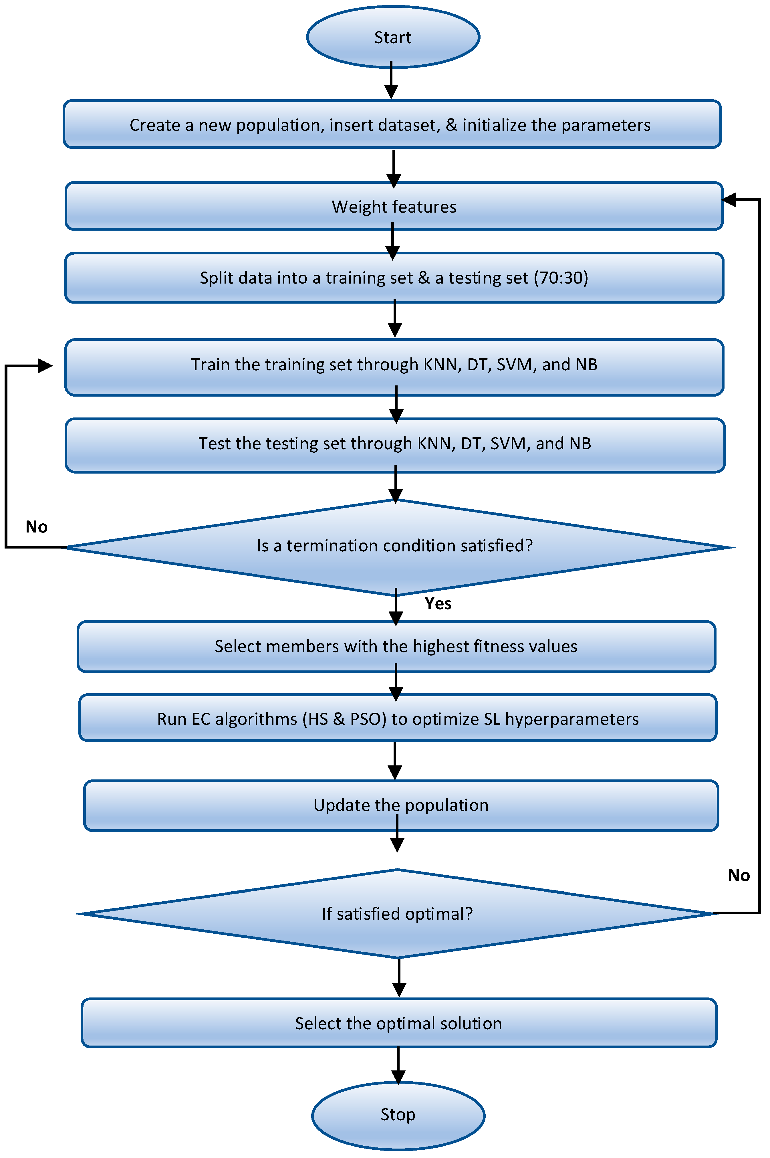Figure 1 illustrates the research method’s flowchart and the algorithm’s implementation in MATLAB. This flowchart includes the following steps: creating the population using four SL algorithms (KNN, DT, SVM, and NB) combined with two EC algorithms (HS and PSO), incorporating the Feature Weighting approach and using four performance metrics (MSE, RMES, MAE, and R²), and each method (SL combined with EC algorithms) received a score with a Total Ranking Score technique. Initializing the parameters and generating a new population are the first steps in the flowchart. Next, we use the Feature Weighting (FW) method to assess each feature’s significance, give it a suitable weight, and calculate how relevant it is to the model. Every feature instance’s value is multiplied throughout the FW process, and the feature instances are then sorted by their values [30]. The chosen features are often equally significant for predicting the outcome.

However, some features with a more significant weight might affect the performance and accuracy of the entire algorithm and the outcomes. We then split the data into two parts: 70% of the dataset for training and 30% for testing. We applied four different SL algorithms (KNN, DT, SVM, and NB) to predict the costs of the model and then selected the precise algorithms for the model. Two EC algorithms (HS and PSO) were then utilized to improve the hyperparameters of the SL algorithms and enhance the SL algorithms’ performance. Next, we used four performance metrics to access the model: the Mean Square Error (MSE), the Root Mean Square Error (RMSE), the Mean absolute error (MAE), and the correlation coefficient (R²). This method produced the following outputs: five FWs (one weight for each feature) for objective 1 and four performance metrics for objectives 1 and 2.

The Total Ranking Score (TRS), a score-based ranking methodology, was utilized to identify which prediction algorithms were the most reliable. Based on the estimated MSE, RMES, MAE, and R² values, the TRS assigned a score to each approach and five feature weight values in objectives 1 and 2. After that, each method’s ranking position was determined by adding all the scores.

4. Proposed Optimization Multi-Function BT-Enabled PSC Model

This section defines the nonlinear BT-enabled PSC cost model with two objectives. The proposed model is a nonlinear multi-function approach to evaluate Pharmaceutical Supply Chains with their uncertainties in demand parameters. The model is designed to estimate the total costs of BT-enabled PSCs, including considering the unmet demand in the pharmaceutical system. The mathematical model with two objectives includes the Raw Materials cost, Finished Products cost, Shortage–Surplus cost, Blockchain Installation cost, Blockchain Transaction cost, and the Unsatisfied Demand of product families. Equation (1) expresses the multi-function BT-enabled PSC model.

Obj₁ = [C_PCS] + [C_Blockchain]

Obj₁ = [C_{raw_materials} + C_{finished_products} + C_{shortage_surplus}] + [C_{BT_Installation} + C_{BT_Transaction}]

$$\begin{gathered} \mathbf{Min} {\mathbf{Obj}}_{\mathbf{1}}=\mathrm{M}\mathrm{i}\mathrm{n}\left({\sum }_{i=1}^{\mathrm{M}}[C_{i,raw\_materials}+C_{i,finished\_products}+C_{i,shortage\_surplus}+ \\ {C}_{i,BT\_Installation}{+C}_{i,BT\_Transaction}]\right) \end{gathered}$$

$$\mathbf{Min} {\mathbf{Obj}}_{\mathbf{2}}=\mathrm{Min} (\mathrm{Max} {\sum }_{i=1}^{\mathrm{M}}[D_i,\mathrm{uncertainty}]$$

(1)

Table 1. Parameters and constraints for all parts of the BT-enabled PSC cost model.

Parameters	Explanation	Constraints
M	Number of products controlled in the PSC variables	35
qi	Order quantity for the ith product per year (i = 1, 2, 3, …, M)	50 ≤ qi ≤ 100 (integer)
di	The average demand for the ith product per year	45 ≤ di ≤ 115 (integer)
n	Total number of lots of M products delivered by the pharmaceutical system to the client per year	50 ≤ n ≤ 100 (integer)
Iv	The interest rate for calculating the opportunity interest loss for the pharmaceutical system due to delayed payment per year	Iv = 0.02
Tc	Common trade credit period for all products offered by the pharmaceutical system in years	0.1
hvi	Holding cost for the ith finished product per year	20 ≤ hvi ≤ 40
si	Set-up cost for the ith finished product per year	12 ≤ si ≤ 25
pi	The production rate for the ith finished product	45 ≤ pi ≤ 115 (integer)
bi	The purchase price per unit for the ith product	80 ≤ bi ≤ 150
pci	Production cost for a product i per year	25 ≤ pci ≤ 50
dci	Expiration rate for the ith finished product	6% ≤ dci ≤ 15%
cdci	Cost of expiry for the ith finished product	25 ≤ cdci ≤ 55
qwi	Replenishment quantity for the ith raw material for the production	20 ≤ qwi ≤ 27
awi	Ordering cost for the ith raw material	15 ≤ awi ≤ 25
hwi	Holding cost per year for the ith raw material	10 ≤ hwi ≤ 15
Fw	Fixed transportation cost for all raw materials per year	3500
vwi	Labor cost for order handling and receipt for the ith raw material per year	16 ≤ vwi ≤ 28
$\mathsf{\beta }$i	$\mathrm{Defect} \mathrm{rate} \mathrm{for} \mathrm{the} i\mathrm{th} \mathrm{raw} \mathrm{material} \mathrm{in} \mathrm{an} \mathrm{order} \mathrm{lot}, \mathsf{\beta }$i $\in$ [0, 1], a random variable	0 ≤ $\mathsf{\beta }$i ≤ 1
rsi	Screening rate per year for the ith raw material	1.04% ≤ rsi ≤ 7.2%
costSi	Shortage cost of unit product type i	10 ≤ costSi ≤ 20
costSUi	Surplus cost of unit product type i	15 ≤ costSUi ≤ 25
z1i	Surplus amount of product i	0 ≤ z1i ≤ 70 (integer) z1i$\ge p_i-$ di
z2i	Shortage amount of product i	0 ≤ z2i ≤ 70/(integer) z2i$\le d_i-$ pi
τi	Comparative importance of product i	1 ≤ τi ≤ 5 (integer)
gWei	The cost paid to the transaction validators and the network (Wei is the unit of ETH)	---
Gu	The amount of Ether as gasUsed per day	$3.86 ≤ Gu × gp ≤ $41.66
gp	Number of gWei to be paid for gasUsed per day
s	The data storage size to store the data	51 TB/yr ≤ s ≤ 99 TB/yr
Cs	Cost storage per year (USD/TB) for Public outbound bandwidth service	$110 × 12 = 1320 $/yr
cfixed	The initial fixed cost per year	860 ≤ cfixed ≤ 1160
conboarding	The Onboarding cost	$180 ≤ conboarding ≤ $260
cmc	The unit Maintenance cost; cmc + cmo is 15–25% of the project value	$230 ≤ cmc + cmo ≤ $550
cmo	The unit Monitoring cost; cmc + cmo is 15–25% of the project value
U	The number of Blockchain users	4
di—pi	The demand uncertainty	≥0

lists the parameters and constraints for the BT-enabled PSC cost model in the pharmaceutical system, including the parts of the mathematical model.

A list of the assumptions is provided below, along with additional notations and assumptions as required [17].

• The PSC comprises a single pharmaceutical system with multiple (M) pharmaceutical products. For the ith product, the pharmaceutical system produces nq_i units at a finite production rate of p_i per unit time in one production cycle.
• For the ith raw materials, all orders are delivered to the pharmaceutical system in one shipment by an external supplier. In other words, the quantity of the ith raw material required for production in each production cycle is instantaneous.
• All expired pharmaceutical products held in inventory by the pharmaceutical system are a constant fraction of the accumulated inventory.
• The pharmaceutical system offers a certain trade credit period (permissible payment delay) for all products to cooperate with clients (like a hospital or a pharmacy) in an integrated strategy. Thus, the customers do not have to pay immediately on receipt of products.
• The credit period T_c is less than the reorder interval for each product, meaning the credit period cannot be longer than when another order is placed. This agrees with the usual practice in healthcare industries.
• Products are all packed, and the number of products is an integer.
• It is assumed that the model uses the available Public Blockchain platform in the market as a hosting platform.
• Node hosting space (cloud storage) stores data; the node number is the copy number of data. We assigned one node in this research (A Blockchain node’s primary job is to confirm the legality of each subsequent batch of network transactions, known as blocks).
• Unsatisfied demand is positive; otherwise, it is zero.

4.1. Cost Elements of A PSC

4.1.1. Raw Materials Cost Elements

The following function, Equation (2), represents the Raw Materials cost in the pharmaceutical system, including the Ordering cost, Holding cost for perfect raw materials, Holding cost for imperfect raw materials, Labor cost for order handling and receipts, and Transportation cost. Equation (2) shows the Cost Order ($\frac{a_{wi }{d}_{i }}{n{q}_{i }}$), the Holding cost for perfect raw materials ($\frac{d_{i }(1-{\mathsf{\beta }}_{i }) q_{wi }{h}_{wi }}{n_{ }{q}_{i }}$), the Holding cost for imperfect raw materials ($\frac{h_{wi } {\mathsf{\beta }}_{i }{q}_{wi }{q_{wi }{d}_{i }}_{ }}{r_{si }{n}_{ }{q}_{i }}$), the Labor cost for order handling and receipt ($\frac{d_{i }{q_{wi }{v}_{wi }}_{ }}{n{q}_{i }}$), and the Transportation cost ($\frac{{\mathrm{F}}_{w }{d}_{i }}{n{q}_{i }}$) [6,17]. It is assumed that each quantity q_wi contains defective raw materials at a rate of $\mathsf{\beta }$_i, which is a random variable.

$${\sum }_{i=1}^{\mathrm{M}}[\frac{a_{wi }{d}_{i }}{n{q}_{i }}+\frac{d_{i }\left(1-{\mathsf{\beta }}_{i }\right)q_{wi }{h}_{wi }}{n_{ }{q}_{i }}+\frac{h_{wi }{\mathsf{\beta }}_{i } q_{wi }{q_{wi }{d}_{i }}_{ }}{r_{si }{n}_{ }{q}_{i }}+\frac{d_{i }{q_{wi }{v}_{wi }}_{ }}{n{q}_{i }}+\frac{{\mathrm{F}}_{w }{d}_{i }}{n{q}_{i }}]$$

(2)

4.1.2. Finished Products Cost Elements

Finished Product i for the pharmaceutical system, which equals the sum of the Set-up cost, Holding cost, Production cost, Expected opportunity interest, and Expiry cost. Equation (3) shows the cost elements of the Finished Products in the pharmaceutical system: the Set-up cost ($\frac{s_{i }{d}_{i }}{n{q}_i}$), the Holding cost ($\frac{h_{vi }{q}_{i }}{2}[n(1-\frac{d_{i }}{p_{i }}$)$-$ 1 $+$ $\frac{2d_{i }}{p_{i }}]$), the Production cost (${d_{i }p}_{ci }{q}_{i }$), the Expected opportunity interest loss per unit time for the product i is I_vb_iT_cd_i, and the Expiry cost (${q_{i }d}_{ci }{c}_{dci }[(\frac{d_{i }}{p_{i }}+(n-1))-\frac{{nd}_{i }}{2p_{i }}]$) [6,17].

$${\sum }_{i=1}^{\mathrm{M}}[\frac{s_{i }{d}_{i }}{n{q}_{i }}+\frac{h_{vi }{q}_{i }}{2}[n(1-\frac{d_{i }}{p_{i }})- 1+ \frac{2d_{i }}{p_{i }}]+ {d_{i }p}_{ci }{q}_{i }+ {\mathrm{I}}_v{b}_i{\mathrm{T}}_{\mathrm{c}}{d}_i+{q_{i }d}_{ci }{c}_{dci }[(\frac{d_{i }}{p_{i }}+(n-1))-\frac{{nd}_{i }}{2p_{i }}]]$$

(3)

4.1.3. Shortage–Surplus Cost Elements

It should be noted that medicine and drug shortages are serious issues in any society, and they are a worldwide problem that governments face because of demand uncertainty and other factors [31]. Equation (4) expresses the Shortage–Surplus cost equation, including Shortage and Surplus costs.

$${\sum }_{i=1}^{\mathrm{M}}[{z^1}_i \times {\mathit{costSU}}_i + {z^2}_i \times {\tau }_i \times {\mathit{costS}}_i]$$

(4)

In Table 1, z¹_i ≥ p_i $-$ d_i and z²_i ≤ d_i $-$ p_i represent a lower bound for the surplus and an upper bound for the shortage of a product, respectively.

4.2. Blockchain Implementation Cost Elements

According to [6], Blockchain Implementation cost (C_Blockchain) consists of two components: Blockchain Transaction cost (C_{BT_Transaction}) and Blockchain Installation cost (C_{BT_Installation}) (Equation (5)). As an alternative for designing and developing a Blockchain platform, it is assumed the model uses the available public Blockchain platform in the market as a hosting platform.

C_Blockchain = C_{BT_Transaction} + C_{BT_Installation}

(5)

Havaeji, Dao, and Wong [6] introduced the C_{BT_Transaction} calculation to pay miners in Equation (6): Total Transaction cost = Gas cost (gasUsed × gasPrice) + Storage cost [32,33,34].

G_u × g_p × 365 + s × C_s

(6)

G_u × g_p is the Gas cost per day, and s × C_s is the Storage cost per year, with a secured cloud-based warehouse storing the actual data off-chain. The IBM Cloud website calculates the Storage cost portion [35]. Table 1 also presents the parameters and constraints for the BT Transaction costs.

Wood [34] mentions Ethereum as a fee for all programmable computation and a kind of currency called Ether (ETH). Proof-of-Work (PoW), like Bitcoin and Ethereum, is the most popular consensus protocol in a public blockchain system [36]. There are two parts to the cost of a typical transaction: gasLimit and gasPrice. Longo et al. [32] state that this calculation must be performed based on the gas used by a transaction to calculate the cost of the Ethereum blockchain. The gasLimit (purchased from the sender’s account balance) is the maximum gas amount that should be used to execute any transaction; any unused gas at the end of a transaction is refunded (at the same rate of purchase) to the sender’s account [6,34]. Wood clarifies that the number of W_ei units to be paid per unit of gas is the gasPrice (a scalar value), which comprises all computation costs incurred due to the transaction’s execution. After submitting a transaction, a given amount of gas is associated with that transaction [32].

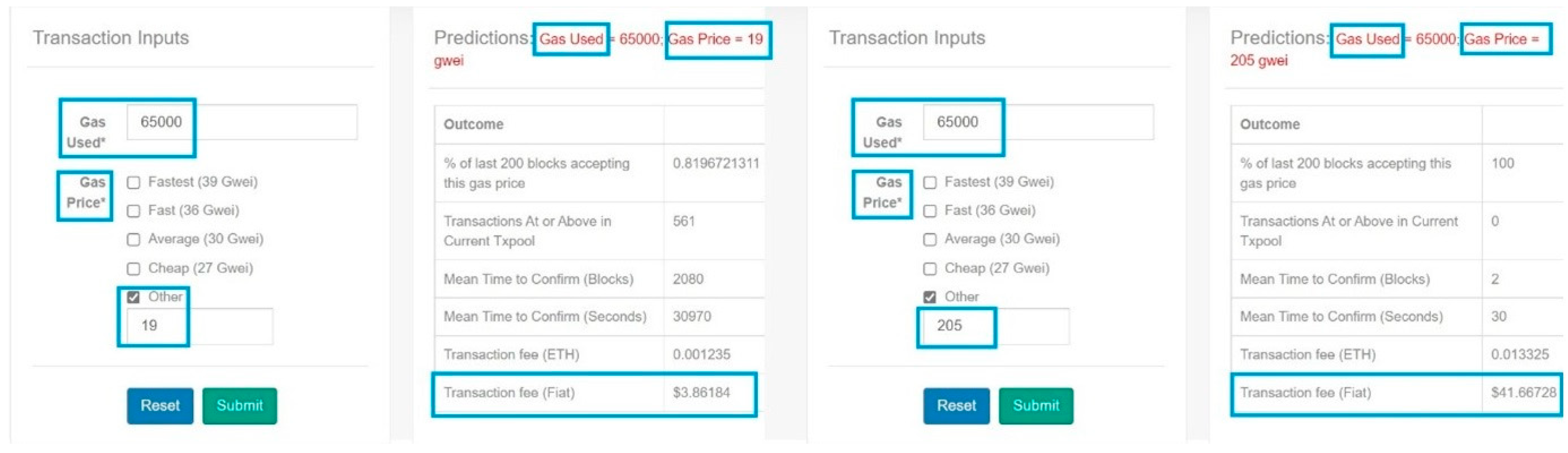
ETH Gas Station calculates G_u × g_p and incentivizes computation within the network [33,37]. The gW_ei is the cost paid to the transaction validators (or the network) for conducting a transaction on the Ethereum Blockchain. The most important aspect is how gW_ei is converted to USD based on the current price of Ethereum by using the ETH Gas Station website [37]. The gasUsed (a scalar value) is the total gas used in transactions. The amount of 65,000, as the amount of gasUsed, and the range of 19 gW_ei to 205 gWei as the gasPrice were selected to calculate the G_u × g_p cost and convert the gW_ei cost to USD via the ETH Gas Station website [37] (Figure 2).

The Blockchain Installation cost (C_{BT_Installation}), or the cost of utilizing BT for PSC, has four cost elements (Equation (7)), including a Fixed cost (c_fixed), Onboarding cost (c_onboarding), Maintenance cost (c_mc), and Monitoring cost (c_mo) [6,38].

$${\sum }_{i=1}^{\mathrm{M}}[c_{\mathit{fixed}} + (c_{\mathit{onboarding}} \times \mathrm{U} + c_{\mathit{mc}} + c_{\mathit{mo}} \times q_i)]$$

(7)

The Onboarding cost (such as onboarding and training) is the cost involved in training suppliers and clients into active users of a product or service. It includes any expenses and costs, which were about integrating new employees into a system so they could learn about and be trained in BT. The c_mc and c_mo costs occur yearly and contribute 15–25 percent of a project’s value [38,39]. Other parameters, including the parameters and constraints for the Blockchain Installation cost, are also shown in Table 1.

4.3. Uncertain Demand Elements

The PSC deals with uncertainty, given that the demand for each medicine product is uncertain and can be influenced by various factors, such as seasonal changes. The uncertain demand occurs when the amount of demand exceeds the available stock. For instance, if a drug price is too low, the demand for that product will be increased, and customers will purchase it from suppliers that can accommodate their demand. This process leads to drug shortages, and so producers should raise their prices and output until supply equals demand and equilibrium is reached. The uncertainty imposes many challenges for modeling and determining optimal solutions. Our model represents the demand uncertainty, as shown in Equation (8), with the input parameters considered under uncertainty [19,24,31,40].

$$\mathrm{Min} {\mathrm{Obj}}_2 = \mathrm{Min} (\mathrm{Max} {\sum }_{i=1}^{\mathrm{M}}[{\mathsf{\tau }}_i[d_i-p_i]])$$

(8)

In Equation (1), the second objective function (Obj₂) aims to reduce the maximum unsatisfied demand of product families, implying an upper constraint for overall unsatisfied demand.

Since the unit’s unfulfilled demand of a low-priority product family is not as important as that of a high-priority product family, this objective is empowered by incorporating the importance parameters π_p to take a balanced attitude towards different product families. To better explain Equation (1), D_{i,uncertainty} is equal to τ_i[d_i $-$ p_i] and should be positive; otherwise, it is zero (D_{i,uncertainty} ≥ 0).

4.4. Optimization Multi-Function for BT-Enabled PSC

The integrated expected total cost for the multi-function BT-enabled PSC model for products in a pharmaceutical system can be expressed in Equation (9) as the sum of the expected total costs of the following components: Raw Materials cost (Ordering cost, Holding cost for perfect raw materials, Holding cost for imperfect raw materials, Labor cost for order handling and receipt, and Transportation cost) (Equation (2)), Finished Products cost (Set-up cost, Holding cost, Production cost, Expected opportunity interest, and Expiry cost) (Equation (3)), Shortage-Surplus cost (Shortage cost and Surplus cost) (Equation (4)), Blockchain Installation cost (Fixed cost, Onboarding cost, Maintenance cost, and Monitoring cost (Equation (7)), and Blockchain Transaction cost (Gas cost and Storage cost) (Equation (6)). The second objective is the Unsatisfied Demand, given by Equation (8).

$$\begin{gathered} \mathbf{Min} {\mathbf{Obj}}_{\mathbf{1}}={\sum }_{i=1}^{\mathrm{M}}[\frac{a_{wi }{d}_{i }}{n{q}_{i }}+\frac{d_{i }\left(1-{\mathsf{\beta }}_{i }\right)q_{wi }{h}_{wi }}{n_{ }{q}_{i }}+\frac{h_{wi } {\mathsf{\beta }}_{i }{q}_{wi }{q_{wi }{d}_{i }}_{ }}{r_{si }{n}_{ }{q}_{i }}+\frac{d_{i }{q_{wi }{v}_{wi }}_{ }}{n{q}_{i }}+\frac{{\mathrm{F}}_{w }{d}_{i }}{n{q}_{i }}+\frac{s_{i }{d}_{i }}{n{q}_{i }} \\ +\frac{h_{vi }{q}_{i }}{2}[n(1-\frac{d_{i }}{p_{i }} )- 1+ \frac{2d_{i }}{p_{i }}]+ {d_{i }p}_{ci }{q}_{i }+ {\mathrm{I}}_v{b}_i{\mathrm{T}}_{\mathrm{c}}{d}_i+{q_{i }d}_{ci }{c}_{dci }[(\frac{d_{i }}{p_{i }}+(n-1))- \\ \frac{{nd}_{i }}{2p_{i }}]+ {z^1}_i \times {\mathit{costSU}}_i + {z^2}_i \times {\tau }_i \times {\mathit{costS}}_i+C_{\mathit{fixed}} + (C_{\mathit{onboarding}} \times \mathrm{U} + C_{\mathit{mc}} + C_{\mathit{mo}}) \times q_{\mathit{i}}] + {\mathrm{G}}_{\mathrm{u}} \times \\ {g}_p \times 365 + s \times {\mathrm{C}}_{\mathrm{s}} \end{gathered}$$

$$\mathbf{Min} {\mathbf{Obj}}_{\mathbf{2}} \mathrm{Min} (\mathrm{Max} {\sum }_{i=1}^{\mathrm{M}}[{\mathsf{\tau }}_i[d_i-p_i]])$$

(9)

5. Results

The numerical examples considered in this study validate the proposed multi-function BT-enabled PSC model in this section. The model is designed to minimize the total costs of BT-enabled PSC, or objective 1, and the unmet demand in the pharmaceutical company, objective 2. This section displays the findings, the performance metrics of eight algorithms on the produced datasets in objectives 1 and 2, and the weights of the objective 1 cost features. The numerical dataset examined here validates the multi-function model and demonstrates the performance of our research method. We used HS and PSO (EC algorithms) to enhance the outputs and optimize the hyperparameters of the KNN, DT, SVM, and NB SL algorithms. This combination provides eight algorithms to reduce prediction errors: HS-KNN, HS-DT, HS-SVM, HS-NB, PSO-KNN, PSO-DT, PSO-SVM, and PSO-NB. To evaluate the efficiency of the proposed algorithms, four performance metrics were used: the MSE, RMSE, MAE, and R². In objective 1, the FW technique was also employed to determine the influencing features for the produced dataset. There was no need to use FW for objective 2 because it only has one component. Without affecting the basic data content, FW plays a key role in the analysis. After data generation, we designed the model, executed the proposed methodology, and used MATLAB software to evaluate the multi-function BT-enabled PSC model. In eighty runs (410 + 410), we examined the “average” of the four performance metrics in objectives 1 and 2 and the “average” of the weight of the cost features in objective 1. We used averages to analyze the results since the runs have different outputs, and the average provides us with stability and dependability in behavioral data. Each run had a maximum of 1000 iterations. Next, rather than assessing the predictions of the multi-function BT-enabled PSC model in each run, we compared the average of every ten runs. Lastly, the TRS technique was utilized to identify the most reliable forecasting algorithms for the multi-function BT-enabled PSC model.

Table 2. Examining objectives 1 and 2 in 10 runs using feature weighting and performance indicators for HS linked with four SL algorithms.

		Objective 1									Objective 2
HS_KNN	Run	Feature Weighting					Performance Metrics				Performance Metrics
		W_(Raw_Materials)	W_(Finished_Products)	W_(Shortage_Surplus)	W_(BT_Installation)	W_(BT_Transaction)	MSE	RMSE	MAE	R2	MSE	RMSE	MAE	R2
	1	0.31	1	0.83	1	1	447,578,659.37	21,156.05	15,225.04	0.99	24,710.22	157.19	122.09	0.006
	2	0.321	0.978	0.911	0.874	0.568	12,216,876,173.60	110,529.97	83,903.98	0.991	24,508.02	156.55	120.55	0.003
	3	0.493	0	0.797	0	0.253	2,584,577,237,772.87	1,607,662.04	1,428,615.72	0.033	23,231.68	152.41	117.72	0.006
	4	0.855	0	0.239	0	0.067	2,559,565,339,629.15	1,599,864.16	1,316,755.65	0.082	8411.63	91.71	59.56	0.132
	5	0.513	0.332	0.087	0.358	0.892	24,544,114,160.46	156,665.61	112,810.15	0.983	4820.3	69.42	39.76	0.474
	6	0.068	0.974	1	1	0.938	592,467,081.45	24,340.64	16,459.35	0.999	3021.13	54.96	34.6	0.554
	7	0.0989	0.994	1	1	1	558,779,878.15	23,638.52	16,243.51	0.999	13,822.96	117.57	88.13	0.195
	8	1	0.934	0.695	0.848	1	517,518,033.07	22,749.0227	16,312.7089	0.999	23,441.02	153.10	117.82	0.004
	9	1	0.940	0.685	0.915	1	18,935,746,767.50	137,607.21	101,185.10	0.986	13,012.55	114.07	85.42	0.205
	10	0	0.548	0.479	0.584	0.672	414,695,195.67	20,364.0663	15,134.7278	0.999	7351.13	85.73	59	0.0302
Average		0.46	0.67	0.67	0.65	0.73	520,237,035,335.13	283,604.18	227,843.03	0.86	14,633.06	115.27	84.47	0.16
		Objective 1									Objective 2
HS_DT	Run	Feature Weighting					Performance Metrics				Performance Metrics
		W_(Raw_Materials)	W_(Finished_Products)	W_(Shortage_Surplus)	W_(BT_Installation)	W_(BT_Transaction)	MSE	RMSE	MAE	R2	MSE	RMSE	MAE	R2
	1	0.194	0.257	0.838	0.271	0.248	487,814,443.56	22,086.52	16,297.92	0.999	22,777.09	150.92	114.31	0.010
	2	0	0.898	0	1	0	2,499,618,098.92	49,996.18	35,512.63	0.998	19,404.58	139.30	106.21	0.004
	3	0	0.866	0	0.691	0	2,008,075,275.94	44,811.55	32,162.61	0.998	19,118.08	138.26	105.64	0.004
	4	0	1	0	0.572	0	2,222,526,522.60	47,143.67	34,027.37	0.998	18,782.17	137.04	106.68	0.010
	5	0.878	0.299	0.714	1	0	2,124,057,520.85	46,087.49	33,848.02	0.998	10,892.02	104.36	77.62	0.313
	6	0	0.154	0	1	0	2,407,898,995.12	49,070.34	35,782.17	0.998	19,876.76	140.98	106.38	0.002
	7	0	0.406	0	0.896	0	2,268,558,510.16	47,629.38	34,306.15	0.998	19,171.03	138.45	105.52	0.006
	8	0.356	0.012	0.957	1	0	2,121,641,968.13	46,061.28	34,345.41	0.998	9716.27	98.57	73.83	0.341
	9	1	0.108	1	0.500	0	2,425,609,238.87	49,250.47	35,790.56	0.998	10,676.44	103.32	77.43	0.304
	10	0.166	0.044	0.392	0.784	0	2,760,284,205.16	52,538.40	36,269.32	0.998	10,342.51	101.69	74.97	0.324
Average		0.26	0.40	0.39	0.77	0.02	2,132,608,477.93	45,467.53	32,834.22	1.00	16,075.70	125.29	94.86	0.13
		Objective 1									Objective 2
HS_SVM	Run	Feature Weighting					Performance Metrics				Performance Metrics
		W_(Raw_Materials)	W_(Finished_Products)	W_(Shortage_Surplus)	W_(BT_Installation)	W_(BT_Transaction)	MSE	RMSE	MAE	R2	MSE	RMSE	MAE	R2
	1	0.231	0.981	0.642	0.076	0.744	8,216,337,569.52	90,644.01	78,810.96	0.999	1343.01	36.64	27.23	0.713
	2	0.679	0	0.020	0.003	0.153	6,757,738,172.25	82,205.46	70,810.95	0.997	2076.14	45.56	33.16	0.588
	3	0.126	0.504	0.799	0.198	0.0431	4,785,591,120.97	69,177.96	63,238.64	0.999	2076.14	45.56	33.16	0.588
	4	0.001	0.599	0.818	0.208	0.115	5,539,994,619.11	74,431.14	63,613.45	0.999	1764.26	42.00	33.29	0.727
	5	0.993	0.287	1	0.243	0.174	6,618,206,320.17	81,352.35	64,946.07	0.995	2887.11	53.73	45.25	0.579
	6	0.689	0.725	0.533	0.104	0.126	6,964,170,744.91	83,451.60	72,470.90	0.999	1764.26	42.00	33.29	0.727
	7	0.064	0.172	1	0.027	0.68	6,600,773,868.49	81,245.14	68,273.45	0.999	8108.04	90.04	73.82	0.346
	8	0.750	0.016	0.035	0.007	0.534	6,002,777,653.01	77,477.59	68,913.88	0.999	2155.18	46.42	37.33	0.814
	9	0.460	0.031	0.787	0.031	0.432	4,877,903,687.16	69,841.99	57,241.79	0.996	5128.06	71.61	53.09	0.535
	10	0.679	0	0.020	0.003	0.153	6,757,738,172.25	82,205.46	70,810.95	0.997	2934.60	54.17	36.95	0.773
Average		0.47	0.33	0.57	0.09	0.32	6,312,123,192.78	79,203.27	67,913.10	1.00	3023.68	52.77	40.66	0.64
		Objective 1									Objective 2
HS_NB	Run	Feature Weighting					Performance Metrics				Performance Metrics
		W_(Raw_Materials)	W_(Finished_Products)	W_(Shortage_Surplus)	W_(BT_Installation)	W_(BT_Transaction)	MSE	RMSE	MAE	R2	MSE	RMSE	MAE	R2
	1	0.968	0.001	0.987	0	0.047	757.59	27.52	20.52	1	2618.22	51.16	34.57	0.809
	2	0.576	0.008	0.966	0.001	0.403	115.42	10.74	9.53	1	1713.43	41.39	34.15	0.634
	3	1	0.002	0.982	0	0.146	193.52	13.91	11.66	1	2256.35	47.50	36.31	0.551
	4	0.986	0.001	0.905	0	0.169	197.89	14.06	11.57	1	2141.78	46.27	31.92	0.655
	5	0.761	0.002	0.650	0	0.039	164.36	12.82	10.43	1	1959.94	44.27	33.18	0.649
	6	0.871	0.003	0.924	0	0.955	162.34	12.74	10.87	1	2918.73	54.02	44.42	0.584
	7	0.926	0.006	0.920	0.001	0.728	185.71	13.62	11.60	1	4111.33	64.11	47.80	0.402
	8	0.950	0.003	0.527	0	0.080	217.95	14.76	12.86	1	2566.81	50.66	41.41	0.447
	9	0.990	0.002	0.355	0	0.034	130.74	11.43	8.04	1	2451.95	49.51	37.18	0.704
	10	0.576	0.008	0.966	0.001	0.403	115.42	10.74	9.53	1	1323.14	36.37	29.23	0.694
Average		0.86	0.00	0.82	0.00	0.30	224.09	14.23	11.66	1.00	2406.17	48.53	37.02	0.61

,

Table 3. Performance indicators for HS linked with four SL algorithms were utilized to assess objectives 1 and 2.

	Objective 1				Objective 2
	Performance Metrics				Performance Metrics
Methods	Ave_MSE	Ave_RMSE	Ave_MAE	Ave_R2	Ave_MSE	Ave_RMSE	Ave_MAE	Ave_R2
HS_KNN	520,237,035,335.13	283,604.18	227,843.03	0.86	14,633.06	115.27	84.47	0.16
HS_DT	2,132,608,477.93	45,467.53	32,834.22	1.00	16,075.70	125.29	94.86	0.13
HS_SVM	6,312,123,192.78	79,203.27	67,913.10	1.00	3023.68	52.77	40.66	0.64
HS_NB	224.09	14.23	11.66	1.00	2406.17	48.53	37.02	0.61

,

Table 4. FW criteria for four SL algorithms optimized by HS in objective 1.

	Feature Weighting
Methods	Max_Ave_Weighting	Min_Ave_Weighting
HS_KNN	W_(BT_Transaction) = 0.73	W_(Raw_Materials) = 0.46
HS_DT	W_(BT_Installation) = 0.77	W_(BT_Transaction) = 0.02
HS_SVM	W_(Shortage_Surplus) = 0.57	W_(BT_Installation) = 0.09
HS_NB	W_(Raw_Materials) = 0.86	W_(Finished_Products) & W_(BT_Installation) = 0.00

,

Table 5. Evaluation of objectives 1 and 2 using feature weighting and performance indicators for PSO linked with four SL algorithms across ten runs.

		Objective 1									Objective 2
PSO_KNN	Run	Feature Weighting					Performance Metrics				Performance Metrics
		W_(Raw_Materials)	W_(Finished_Products)	W_(Shortage_Surplus)	W_(BT_Installation)	W_(BT_Transaction)	MSE	RMSE	MAE	R2	MSE	RMSE	MAE	R2
	1	0	0.825	0	1	1	549,741,219.89	23,446.5609	16,634.91	0.999	23,806.25	154.29	117.60	0.011
	2	0.533	0.744	0.322	0.817	0.884	491,607,040.75	22,172.21	15,688.57	0.999	22,455.19	149.85	114.24	0.009
	3	0.767	0.007	0.102	0.018	0.786	61,527,504,303.02	248,047.38	185,904.62	0.959	19,758.51	140.56	106.62	0.042
	4	0.676	0.049	0.794	0.045	0	525,110,440.86	22,915.28	17,221.68	0.999	23,954.87	154.77	118.47	0.009
	5	0.516	0.560	0.111	0.907	0.281	550,748,692.11	23,468.03	17,092.62	0.999	24,544.10	156.66	122.29	0.0079
	6	1	1	0.617	1	0.627	454,654,767.36	21,322.63	15,340.97	0.999	24,004.42	154.93	118.78	0.006
	7	1	0.186	0	0.080	0.942	10,745,095,521.78	103,658.55	79,592.31	0.987	12,554.8	112.04	79.13	0.103
	8	0	0.554	1	0.702	0.470	431,096,960.34	20,762.87	15,099.64	0.999	6669	81.66	59.33	0.226
	9	1	1	0.543	1	0.616	454,972,132.96	21,330.07	15,345.73	0.999	24,561.92	156.72	122.34	0.007
	10	0.886	0.047	1	0.152	0	742,284,495.02	27,244.89	20,085.31	0.999	20,796.63	144.21	109.21	0.020
Average		0.64	0.50	0.45	0.57	0.56	7,647,281,557.41	53,436.85	39,800.64	0.99	20,310.57	140.57	106.80	0.04
		Objective 1									Objective 2
PSO_DT	Run	Feature Weighting					Performance Metrics				Performance Metrics
		W_(Raw_Materials)	W_(Finished_Products)	W_(Shortage_Surplus)	W_(BT_Installation)	W_(BT_Transaction)	MSE	RMSE	MAE	R2	MSE	RMSE	MAE	R2
	1	0.074	0.453	0.252	0.142	0	2,124,057,520.85	46,087.49	33,848.02	0.998	10,892.02	104.36	77.62	0.313
	2	0.333	0.322	0.811	0.069	0.406	66,808,063,437.00	258,472.55	196,228.98	0.952	10,643.44	103.16	77.68	0.337
	3	0.232	0.304	0.073	0.088	0	2,222,537,815.15	47,143.79	34,199.82	0.998	9340.04	96.64	72.67	0.351
	4	0.917	0.778	0.670	0.210	0	68,611,472,474.87	261,937.91	202,530.73	0.953	2361.72	48.59	29.84	0.694
	5	0.225	1	0.277	1	0	2,464,171,102.89	49,640.41	35,610.29	0.998	3199.95	56.56	34.61	0.409
	6	0	0.145	0.627	0.285	0	50,446,994,254.48	224,604.08	166,066.93	0.957	2678.00	51.74	35.21	0.654
	7	0	1	0.169	0.315	0	68,200,434,557.48	261,152.12	201,638.36	0.925	2920.60	54.04	40.28	0.552
	8	0.602	0.248	0.020	0.947	0.061	65,259,550,220.65	255,459.48	194,744.85	0.946	3266.07	57.14	41.86	0.537
	9	0.789	0.134	0.134	0.751	0	2,331,651,357.13	48,287.17	35,532.25	0.998	10,094.09	100.46	74.92	0.313
	10	0.428	0.428	0.208	0.011	0.948	2,353,131,810.38	48,509.09	35,571.26	0.998	10,475.52	102.35	76.50	0.325
Average		0.36	0.48	0.32	0.38	0.14	33,082,206,455.09	150,129.41	113,597.15	0.97	6587.15	77.50	56.12	0.45
		Objective 1									Objective 2
PSO_SVM	Run	Feature Weighting					Performance Metrics				Performance Metrics
		W_(Raw_Materials)	W_(Finished_Products)	W_(Shortage_Surplus)	W_(BT_Installation)	W_(BT_Transaction)	MSE	RMSE	MAE	R2	MSE	RMSE	MAE	R2
	1	0.834	0.994	0.999	0.340	0.535	6,481,651,810.93	80,508.70	72,188.64	0.999	293,747.64	541.98	437.60	0.136
	2	1	0.527	0.283	0.184	0.966	5,547,584,998.00	74,482.11	69,169.55	0.999	3507.26	59.22	48.12	0.745
	3	0.935	1	0.481	0.347	1	3,605,444,643.76	60,045.35	55,331.24	0.999	3373.98	58.08	48.39	0.572
	4	0.916	1	0.680	0.351	1	4,514,645,983.04	67,191.11	61,008.17	0.999	3715.10	60.95	51.35	0.354
	5	0.783	0.832	0.080	0.181	0.862	5,844,285,150.30	76,447.92	68,615.39	0.999	1644.43	40.55	31.86	0.699
	6	0.530	0.340	1	0.134	0	5,986,270,734.82	77,370.99	66,270.24	0.999	3927.42	62.66	52.17	0.651
	7	0.490	0.305	0.999	0.106	1	4,348,863,443.90	65,945.91	57,060.60	0.999	2011.16	44.84	34.05	0.650
	8	0.679	0.107	0.392	0.037	0.313	4,509,807,347.28	67,155.09	58,613.10	0.999	3655.66	60.46	47.21	0.504
	9	1	0.281	0.282	0.108	0.617	6,022,445,081.15	77,604.41	66,322.34	0.999	1,170,745.01	1082.00	919.48	0.0669
	10	0.895	0.624	0.413	0.245	0.753	4,374,513,944.83	66,140.10	57,651.87	0.999	1,149,307.12	1072.05	753.85	0.174
Average		0.81	0.60	0.56	0.20	0.70	5,123,551,313.80	71,289.17	63,223.11	1.00	263,563.48	308.28	242.41	0.46
		Objective 1									Objective 2
PSO_NB	Run	Feature Weighting					Performance Metrics				Performance Metrics
		W_(Raw_Materials)	W_(Finished_Products)	W_(Shortage_Surplus)	W_(BT_Installation)	W_(BT_Transaction)	MSE	RMSE	MAE	R2	MSE	RMSE	MAE	R2
	1	0.019	0.091	0.883	0.244	0.335	27,165.54	164.81	139.53	1	4374.03	66.13	54.98	0.438
	2	1	0.004	1	0.001	1	241.74	15.54	13.24	1	2335.18	48.32	40.55	0.60
	3	1	0.029	0.995	0	0.999	158.73	12.59	10.48	1	1622.74	40.28	33.03	0.679
	4	0.336	0.472	1	0.377	0.582	385,352.01	620.76	517.70	1	4244.30	65.14	55.06	0.255
	5	1	0.529	0.990	0.965	1	653,210.23	808.21	583.32	1	9377.69	96.83	69.14	0.243
	6	1	0.005	1	0.001	0.085	80.76	8.98	7.00	1	1874.46	43.29	36.17	0.560
	7	0.992	0.464	0.989	0.026	0.650	754.26	27.46	22.41	1	3180.67	56.39	52.21	0.116
	8	0.558	0	0.942	0	1	147.15	12.13	9.87	1	2392.15	48.90	35.94	0.554
	9	0.992	0.001	0.984	0	0.157	277.38	16.65	13.96	1	1929.62	43.92	34.37	0.638
	10	0.750	0.015	0.999	0	0.656	264.05	16.24	13.20	1	5488.47	74.08	59.06	0.310
Average		0.76	0.16	0.98	0.16	0.65	106,765.19	170.34	133.07	1.00	3681.93	58.33	47.05	0.44

,

Table 6. Performance indicators for PSO linked with four SL algorithms for assessing objectives 1 and 2.

	Objective 1				Objective 2
	Performance Metrics				Performance Metrics
Methods	Ave_MSE	Ave_RMSE	Ave_MAE	Ave_R2	Ave_MSE	Ave_RMSE	Ave_MAE	Ave_R2
PSO_KNN	7,647,281,557.41	53,436.85	39,800.64	0.99	20,310.57	140.57	106.80	0.04
PSO_DT	33,082,206,455.09	150,129.41	113,597.15	0.97	6587.15	77.50	56.12	0.45
PSO_SVM	5,123,551,313.80	71,289.17	63,223.11	1.00	263,563.48	308.28	242.41	0.46
PSO_NB	106,765.19	170.34	133.07	1.00	3681.93	58.33	47.05	0.44

,

Table 7. In objective 1, the FW criteria for PSO were linked with four SL algorithms.

	Feature Weighting
Methods	Max_Ave_Weighting	Min_Ave_Weighting
PSO_KNN	W_(Raw_Materials) = 0.64	W_(Shortage_Surplus) = 0.45
PSO_DT	W_(Finished_Products) = 0.48	W_(BT_Transaction) = 0.14
PSO_SVM	W_(Raw_Materials) = 0.81	W_(BT_Installation) = 0.20
PSO_NB	W_(Shortage_Surplus) = 0.98	W_(Finished_Products) & W_(BT_Installation) = 0.16

,

Table 8. Using the performance indicators in objectives 1 and 2 to rank eight chosen algorithms based on their TRS ratings.

		Objective 1				Objective 2
		Performance Metrics				Performance Metrics				TRS	Rank
Method		Ave_MSE	Ave_RMSE	Ave_MAE	Ave_R2	Ave_MSE	Ave_RMSE	Ave_MAE	Ave_R2
HS_KNN		520,237,035,335.13	283,604.18	227,843.03	0.86	14,633.06	115.27	84.47	0.16
HS_DT		2,132,608,477.93	45,467.53	32,834.22	1.00	160,75.70	125.29	94.86	0.13
HS_SVM		6,312,123,192.78	79,203.27	67,913.10	1.00	3023.68	52.77	40.66	0.64
HS_NB		224.09	14.23	11.66	1.00	2406.17	48.53	37.02	0.61
PSO_KNN		7,647,281,557.41	53,436.85	39,800.64	0.99	20,310.57	140.57	106.80	0.04
PSO_DT		33,082,206,455.09	150,129.41	113,597.15	0.97	6587.15	77.50	56.12	0.45
PSO_SVM		5,123,551,313.80	71,289.17	63,223.11	1.00	263,563.48	308.28	242.41	0.46
PSO_NB		106,765.19	170.34	133.07	1.00	3681.93	58.33	47.05	0.44
Ranking Score	HS_KNN	1	1	1	5	4	4	4	3	23.00	8
	HS_DT	6	6	6	8	3	3	3	2	37.00	4
	HS_SVM	4	3	3	8	7	7	7	8	47.00	3
	HS_NB	8	8	8	8	8	8	8	7	63.00	1
	PSO_KNN	3	5	5	7	2	2	2	1	27.00	7
	PSO_DT	2	2	2	6	5	5	5	5	32.00	5
	PSO_SVM	5	4	4	8	1	1	1	6	30.00	6
	PSO_NB	7	7	7	8	6	6	6	4	51.00	2

and

Table 9. FW Ranking based on TRS ratings for five algorithms chosen in objective 1.

Objective 1
		Methods								TRS	Rank
Ave_FW		HS_KNN	HS_DT	HS_SVM	HS_NB	PSO_KNN	PSO_DT	PSO_SVM	PSO_NB
W_(Raw_Materials)		0.46	0.26	0.47	0.86	0.64	0.36	0.81	0.76
W_(Finished_Products)		0.67	0.40	0.33	0.00	0.50	0.48	0.60	0.16
W_(Shortage_Surplus)		0.67	0.39	0.57	0.82	0.45	0.32	0.56	0.98
W_(BT_Installation)		0.65	0.77	0.09	0.00	0.57	0.38	0.20	0.16
W_(BT_Transaction)		0.73	0.02	0.32	0.30	0.56	0.14	0.70	0.65
Ranking Score	W_(Raw_Materials)	2	2	4	5	5	3	5	4	30	1
	W_(Finished_Products)	4	4	3	2	2	5	3	2	25	3
	W_(Shortage_Surplus)	4	3	5	4	1	2	2	5	26	2
	W_(BT_Installation)	3	5	1	2	4	4	1	2	22	4
	W_(BT_Transaction)	5	1	2	3	3	1	4	3	22	4

show all of the findings.

5.1. HS Combined with Four SLs

Four performance metrics and the FW method (the weights of five cost features) assessed the multi-function BT-enabled PSC model, which has two objectives. MATLAB was used to run HS together with four SL algorithms (HS-KNN, HS-DT, HS-SVM, and HS-NB) 40 times (each algorithm was run ten times) in 1000 iterations.

Table 2 presents the four performance metrics for four algorithms in objectives 1 and 2, the five weights of the cost features in objective 1, each performance metric’s average value, and the average values for each cost feature in 40 runs. Table 3 and Table 4 are derived from Table 2.

The average of four performance evaluation criteria for each approach in objectives 1 and 2 is summarized and compared in Table 3. In Table 3, HS-NB demonstrates robust behavior in both objectives, with a minimum average of MSE, RMSE, and MAE, and the best average R² of 1 for objective 1, among the four methods. Objective 2 is realized well in both HS-SVM and HS-NB, with R² values of 0.64 and 0.61, respectively. The weakest results in all performance metrics are for HS-KNN in objective 1 and HS-DT in objective 2. Table 3 shows that the HS-NB algorithm performs better at realizing objectives 1 and 2 for the multi-function BT-enabled PSC model than the other suggested algorithms.

Table 4 focuses on the average of the weights of each cost feature using the FW technique for the HS-KNN, HS-DT, HS-SVM, and HS-NB algorithms in objective 1. Objective 2 has just one element, and the FW approach does not work. HS-NB has the most significant average weight for the Raw Materials cost feature (0.86) and the lowest average weight for Finished Products and BT Installation (0.00) among these four approaches. The BT Installation cost feature via the HS-DT algorithm has the second-highest average weight (0.77), and next is the BT Transaction cost feature via the HS-KNN algorithm (0.73). With HS-DT (0.02), the BT Transaction cost feature has the second-lowest average weight. Furthermore, features like the BT Transaction cost and BT Installation fluctuate because the algorithms have different behavior.

5.2. PSO Linked with Four SL Algorithms

In the next step, a PSO linked with four SL algorithms (PSO-KNN, PSO-DT, PSO-SVM, and PSO-NB) was run forty times (ten runs for each) (see Table 5). Next, we used the four performance metrics for the four algorithms in objectives 1 and 2, and the weights of the five cost features in objective 1 to evaluate the multi-function BT-enabled PSC model in these 40 runs (10 runs for each algorithm). In addition, Table 5 shows the average values of the performance metrics and the average values of the weights of the cost features. Table 6 and Table 7 are derived from the data presented in Table 5.

Table 6, from Table 5, displays the average values of four performance indicators used in assessing the PSO algorithm linked with four SL algorithms in objectives 1 and 2. In this table, PSO-NB performs better than the others, with an average R² of 1 and a minimum of Ave-MSE = 106,765.19, Ave-RMSE = 170.34, and Ave-MAE = 133.07 in objective 1. On the other hand, in objective 1, PSO-DT has the lowest score of any performance indicator. In objective 2, PSO-NB also behaves well with all performance metrics among the four methods. As a result, we believe that the PSO-NB findings are more trustworthy than the results produced by the other offered approaches in both objectives.

Table 7 illustrates the average weights of five cost features through the FW method in the PSO-KNN, PSO-DT, PSO-SVM, and PSO-NB algorithms in objective 1. Objective 2 has only one element, which is why the FW approach does not work. PSO-NB provides the minimum and maximum average weights among all cost features. The Shortage–Surplus cost feature receives the highest average weight of 0.98, while the Finished Products and BT Installation cost features have the lowest average weight of 0.16 for the PSO-NB algorithm. The PSO-DT method produced the second-highest average weight for the Finished Products cost feature (0.48). A variation in the average weight of some features in this table is observed, such as Shortage–Surplus with 0.98 and 0.45 by PSO-NB and PSO-KNN, respectively. The algorithms’ varying behavior explains the reason for this variation.

5.3. Determining Reliable Algorithms for Multi-Function BT-Enabled PSC

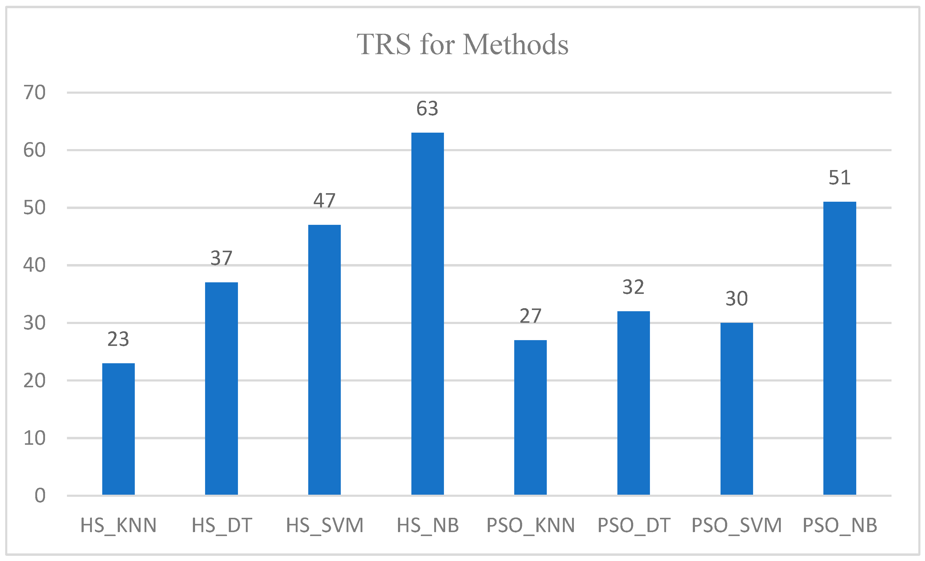
Table 8 displays the TRS of eight algorithms according to the values acquired in objectives 1 and 2 for Ave-MSE, Ave-RMSE, Ave-MAE, and Ave-R2. In objective 2, HS-SVM and HS-NB also behave acceptably with all performance metrics among the eight methods. Objective 1, on the other hand, has good behavior with HS-NB and PSO-NB. To compute the TRS, we allocated the highest scores to the lowest Ave-MSE, Ave-RMSE, and Ave-MAE values, and the highest scores to the highest Ave-R2 values (and inversely). Generally, with a TRS of 63, the HS-NB algorithm performed better than other algorithms, followed by PSO-NB with a TRS of 51, HS-SVM with a TRS of 47, and HS-DT with a TRS of 37. TRS scores of 23 (rank 8th) and 27 (rank 7th) were obtained by HS-KNN and PSO-KNN, respectively.

Table 9 indicates the average weights ranking of the five cost features in objective 1: Raw Materials, Finished Products, Shortage Surplus, BT Installation, and BT Transaction for the HS-KNN, HS-DT, HS-SVM, HS-NB, PSO-KNN, PSO-DT, PSO-SVM, and PSO-NB algorithms. This table provides a suitable average weight and a TRS to demonstrate the significance of each cost feature. In the TRS procedure, the average weight with a higher TRS obtains a more significant priority (and inversely). In general, the Raw Materials cost in objective 1 has the best TRS of 30 for the average weight, followed second by the Shortage–Surplus cost, which has a TRS of 26, and the Finished Products cost, which has a TRS of 25. The minimal TRS for average weight is assigned to the BT Installation and BT Transaction cost features; both rank fourth with TRS = 22.

6. Discussion

This section presents the outcomes of the suggested eight strategies for minimizing the prediction errors of the multi-function BT-enabled PSC model. In this section, we respond to three of the research questions listed in the introduction and discuss the results. As mentioned before, the multi-function BT-enabled PSC model has six components: Raw Materials cost, Finished Products cost, Shortage-Surplus cost, Blockchain Installation cost, Blockchain Transaction cost, and Unsatisfied Demand of product families. Our model has two objectives. The first objective includes Raw Materials cost (Ordering cost, Holding cost for perfect raw materials, Holding cost for imperfect raw materials, Labor cost for order handling and receipt, and Transportation cost), Finished Products cost (Set-up cost, Holding cost, Production cost, Expected opportunity interest, and Expiry cost), Shortage-Surplus cost (Shortage cost and Surplus cost), Blockchain Installation cost (Fixed cost, Onboarding cost, Maintenance cost, and Monitoring cost), and Blockchain Transaction cost (Gas cost and Storage cost). The second objective covers the Unsatisfied Demand. This explanation answers our first research question. Concerning the second study question, we chose those algorithms (among the eight considered here) that performed better in reducing the prediction errors of the multi-function BT-enabled PSC model. Figure 3 displays the TRS for all eight algorithms tested (HS-KNN, HS-DT, HS-SVM, HS-NB, PSO-KNN, PSO-DT, PSO-SVM, and PSO-NB) based on the data reported in Table 8. The efficiency of the eight methods is assessed using four performance indicators (MSE, RMSE, MAE, and R²). The findings of this study suggest that the HS-NB (first position) and PSO-NB (second position) algorithms perform better than the other examined algorithms in terms of reducing model prediction errors. This indicates that NB, when linked with either HS or PSO, is considered the most efficient regression method. The EC algorithms (HS and PSO) are also important in enhancing the hyperparameters of the eight SL algorithms. Moreover, according to the performance metrics’ values and the TRS scores, the SVM, DT, and KNN algorithms, combined with HS and PSO, cannot adequately estimate the costs of the multi-function BT-enabled PSC model. As a result, in response to the second question, we determined that the NB algorithm, when linked with HS and PSO, is the most reliable forecasting algorithm for our multi-function model based on TRS and four performance indicators.

The third research question is to determine the significant components of the model. The only component of objective 2 in the model is the Unsatisfied Demand of product families. On the other hand, objective 1 includes five cost components, and the FW approach measures the importance of the cost features and assigns an appropriate weight to each feature. Figure 4 is derived from Table 9 and shows the TRS for the weights of all the cost components (features) of the multi-function BT-enabled PSC model in Objective 1. These weights estimate the degree of relevance that each feature has for extracting the cost prediction. The results show the Raw Materials cost strongly influences the cost model. The remaining four cost features in Objective 1 have relatively the same weight (Shortage-Surplus cost, Finished Products cost, Blockchain Installation cost, and Blockchain Transaction cost).

As a result, in response to the second question, we determined that the NB algorithm, when linked with HS and PSO, is the most reliable forecasting algorithm for our multi-function model based on TRS and four performance indicators. Researchers in various domains can utilize BT cost formulation (BT Transaction cost and BT Installation cost) in their mathematical models to evaluate the SC costs combined with BT. Another significant contribution of this study is to provide a BT-enabled PSC system with uncertain demand, which occurs when the demand exceeds the available stock. The study is useful because it gives the most reliable prediction algorithms for the multi-function BT-enabled PSC model, the cost components of the BT-enabled PSC system, the degree of relevance of each model component, and the BT components in the PSC model.

Similar to other studies, there are some limitations in this research. Because the use of BT in PSC is a new area of study, our first constraint is the lack of real data. As a result, raw data was collected to validate the suggested multi-function BT-enabled PSC model. Using produced data instead of real data may have an impact on the research’s findings and conclusions. The second constraint pertains to the model’s components, as this research may not include some of the cost components of an actual instance.

At last, further study might lead to developing a multi-function BT-enabled Pharmaceutical Cold Supply Chain model. Pharmaceutical Cold Supply Chain utilizes advanced technology to control the temperature inside cargo containers and storage units. Another idea for future study is to use other EC algorithms to improve the performance of SL algorithms or assess alternative SL algorithms to estimate expenses. Further future research is to investigate how uncertain demand affects cost components of the BT-enabled PSC model. Lastly, future studies may quantify the cost components of private BT, and, therefore, formulate private BT rather than the public BT employed in the present paper.

7. Conclusions

The BT-enabled PSC allows for traceability and transparency in the distribution of pharmaceuticals and stakeholders across the supply chain, which can impact medication quality and end-patient results. This work proposes a mathematical multi-function model for a BT-enabled PSC system to determine the model’s costs. This research is significant because it gives a PSC system with BT costs (BT Transaction cost and BT Installation cost) that may enhance the safety, efficiency, and transparency of medical information exchange in a healthcare system. The research also provides six components of the multi-function model: Raw Materials cost (Ordering cost, Holding cost for perfect raw materials, Holding cost for imperfect raw materials, Labor cost for order handling and receipt, and Transportation cost), Finished Products cost (Set-up cost, Holding cost, Production cost, Expected opportunity interest, and Expiry cost), Shortage–Surplus cost (Shortage cost and Surplus cost), Blockchain Installation cost (Fixed cost, Onboarding cost, Maintenance cost, and Monitoring cost), Blockchain Transaction cost (Gas cost and Storage cost), and Unsatisfied Demand. The combination of two EC algorithms and four SL algorithms yields eight methods for reducing prediction errors, improving the SL algorithms’ hyperparameters, and enhancing the multi-function model. The results show that the HS-NB and PSO-NB algorithms beat the other six algorithms in predicting the costs of the multi-function model with reduced errors. This means that the NB algorithm can estimate the costs of the BT-enabled PSC system better than the KNN, DT, and SVM algorithms. HS-NB and PSO-NB algorithms introduce better performance in comparison with the rest, which means that the HS-NB and PSO-NB algorithms correctly predict the cost of the BT-enabled PSC model better than others. The four performance metrics used in this research (MSE, RMSE, MAE, and R²) help us to evaluate and select the algorithms (through the TRS approach) with better performance. The other six algorithms perform similarly for this comparison, except HS-SVM, which acts better, demonstrating that these algorithms are not a suitable forecasting method for the existing cost model. The results also reveal the Raw Materials cost strongly influences the cost model, more so than the remaining four cost features: Shortage–Surplus cost, Finished Products cost, Blockchain Installation cost, and Blockchain Transaction cost. Moreover, the Raw Materials cost is significant for managers and decision-makers in the context of PSC because it covers Ordering cost, Holding cost for perfect raw materials, Holding cost for imperfect raw materials, Labor cost for order handling and receipt, and Transportation cost. Therefore, the statistical findings on the provided dataset demonstrate that the NB algorithm can produce acceptable results and assign suitable feature weights. These results can assist healthcare service managers in making the correct decisions, regulating financial resources, remaining within budget, evaluating data, and detecting wasteful costs, especially if they decide to apply BT to the system. This research also provides a PSC system with BT that includes demand uncertainty. Managers may utilize the chosen SL algorithms to predict costs with the fewest forecast errors and then evaluate if the new system is beneficial to their organization. The results can be applied in real-world scenarios to improve PSC industries and allow managers in those industries to know how to determine and measure each cost component of the multi-function BT-enabled PSC model to make the best decision before installing the new system. This paper is also recommended to those researchers who work in the PSC industries to develop their organization with BT and evaluate the costs of using BT in PSC.