Methodology for Power Systems’ Emergency Control Based on Deep Learning and Synchronized Measurements

Abstract

Modern electrical power systems place special demands on the speed and accuracy of transient and steady-state process control. The introduction of renewable energy sources has significantly influenced the amount of inertia and uncertainty of transient processes occurring in energy systems. These changes have led to the need to clarify the existing principles for the implementation of devices for protecting power systems from the loss of small-signal and transient stability. Traditional methods of developing these devices do not provide the required adaptability due to the need to specify a list of accidents to be considered. Therefore, there is a clear need to develop fundamentally new devices for the emergency control of power system modes based on adaptive algorithms. This work proposes to develop emergency control methods based on the use of deep machine learning algorithms and obtained data from synchronized vector measurement devices. This approach makes it possible to ensure adaptability and high performance when choosing control actions. Recurrent neural networks, long short-term memory networks, restricted Boltzmann machines, and self-organizing maps were selected as deep learning algorithms. Testing was performed by using IEEE14, IEEE24, and IEEE39 power system models. Two data samples were considered: with and without data from synchronized vector measurement devices. The highest accuracy of classification of the control actions’ value corresponds to the long short-term memory networks algorithm: the value of the accuracy factor was 94.31% without taking into account the data from the synchronized vector measurement devices and 94.45% when considering this data. The obtained results confirm the possibility of using deep learning algorithms to build an adaptive emergency control system for power systems.

1. Introduction

The emergency control (EC) of electrical power systems (EPSs) is an important part of ensuring the reliability of power supply to consumers. For modern EPSs, emergency control is aimed at maintaining small-signal stability (SSS), transient stability (TS), voltage stability, and maintaining the required level of alternating current frequency and the permissible current load of electrical network elements [1]. A separate automation is responsible for each EPS control task by analyzing the parameters of the electrical mode (currents, voltages, active power flows, reactive power flows, etc.) and issuing control actions (CAs) (load shedding, shutdown generators, unloading generators, etc.) followed by the specified logical rules. The operation of automation devices is implemented in stages: the first includes the operation of devices protecting local energy areas and the last includes devices aimed at dividing EPSs.

The EC structure described above shows high reliability and efficiency including the active introduction of renewable energy sources (RESs) [2,3,4,5]. The goal of introducing RESs is to reduce the impact of the electricity sector on global warming [6] by transitioning from traditional power plants running on fossil fuels to low-carbon electricity production by converting solar, wind, tidal, and other renewable energy sources. This goal was partially achieved in many European countries, the USA, India, and China [7].

The key features of RESs are the stochasticity of electricity generation [8,9,10], low inertia [11], and the difficulty of predicting their operating modes. The process of increasing the share of RESs in EPSs is accompanied by the simultaneous dismantling of traditional fossil fuel power units. As a result, the characteristics of the properties of modern EPSs have changed significantly: the speed of transient processes has increased and the accuracy of predicting steady-state processes has decreased.

Features of EPSs are considered in a complex technical system with a significant predominance of digital devices for the analysis, control, and planning of steady-state and transient processes. The digitalization of the electric power industry has led to the accumulation of large amounts of data and the possibility of their processing using machine learning (ML) algorithms [12].

Following the tightening of the rules of the electricity market, there is an active implementation of digital systems that allow for increasing the flow of intersystem active power flows [13,14,15], which reduces the stability margin and increases the likelihood of developing an accident with EPS division.

Table 1 provides an analysis of the features of modern EPSs.

Table 1. Features of modern EPSs.

Specificity	Merits	Drawbacks
A significant share of RESs	Reducing the impact of the electricity generation process on the environment	Increased speed of transient processes, increased uncertainty of EPS operations
Tightening the rules of the electricity market	Increasing the financial efficiency of EPSs	Reduced stability margin
A high degree of digitalization	Possibility of developing and implementing fundamentally new algorithms for managing and analyzing EPS operations	Increased complexity and labor costs for maintaining digital systems

The described features of modern EPSs place new demands on traditional EC systems in terms of adaptability, accuracy, and speed. Traditional EC systems are based on one of two principles:

• The choice of CA is carried out based on a predetermined logic, considering the worst-case scenario for accident development;
• The choice of CA is carried out based on the actual operating mode of the EPS in a cyclic mode based on a mathematical model of the protected section of the electrical network.

To implement both EC principles, a pre-prepared list of examined accidents is used. This list is compiled manually based on operating experience and EPS accident statistics. In addition, the logic of operation of traditional EC devices is based on strictly deterministic approaches by implying a numerical analysis of a system of differential-algebraic equations that describe the mathematical model of the protected EPS. These features of traditional EC devices do not meet the requirements of modern EPSs in terms of speed and adaptability.

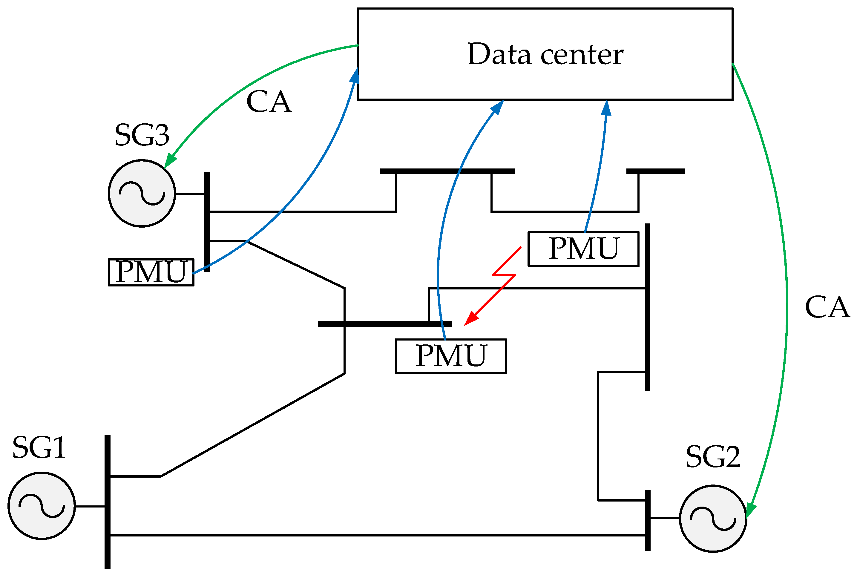
The development of computer technology, the theory of mathematical statistics, ML methods, as well as the active implementation of synchronized vector measurement devices (PMUs) make it possible to develop an adaptive EC EPS system based on big data classification algorithms using obtained PMUs during the registration of transient processes. This approach allows us to ensure the required adaptability and speed of CA selection.

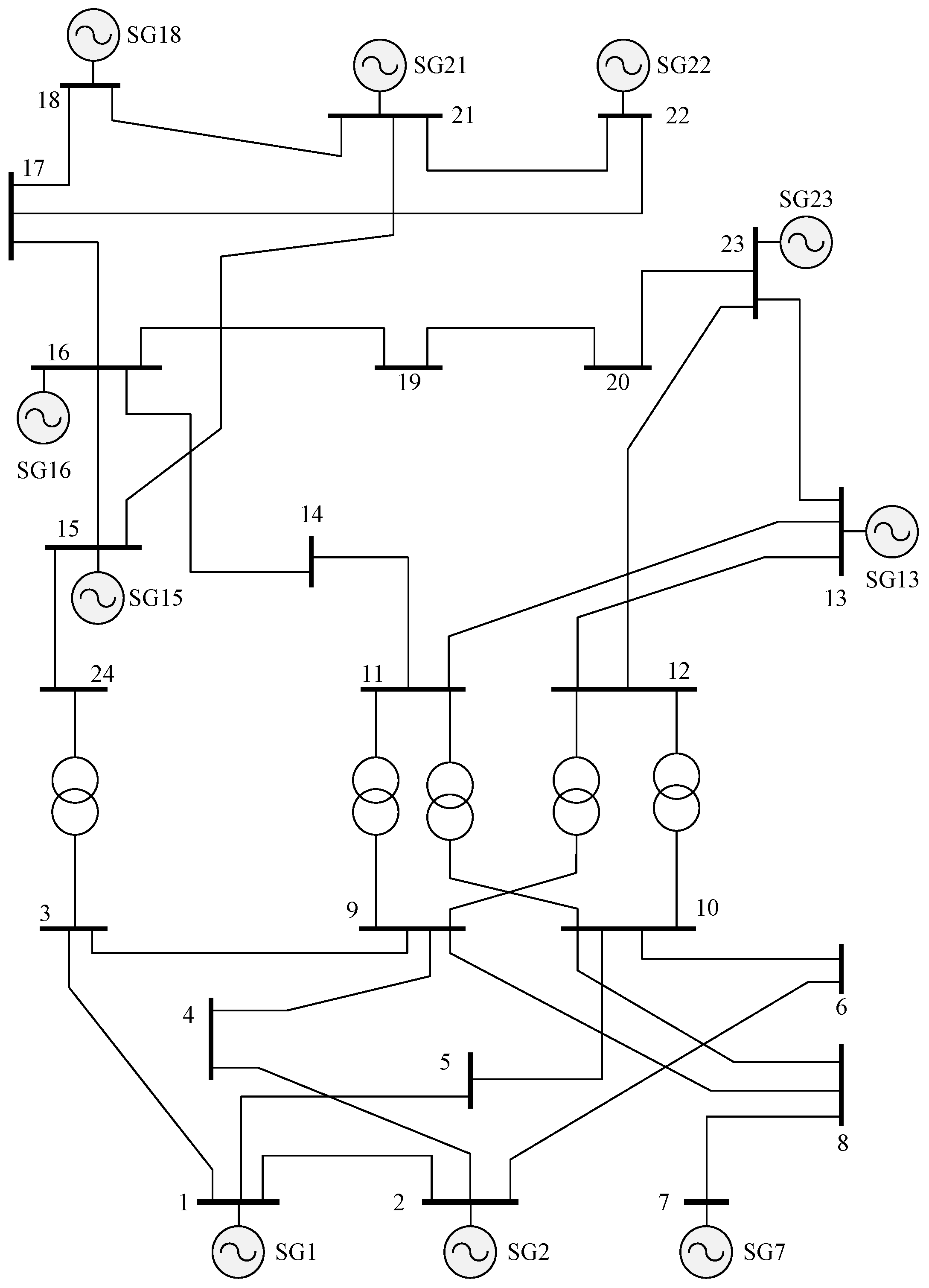
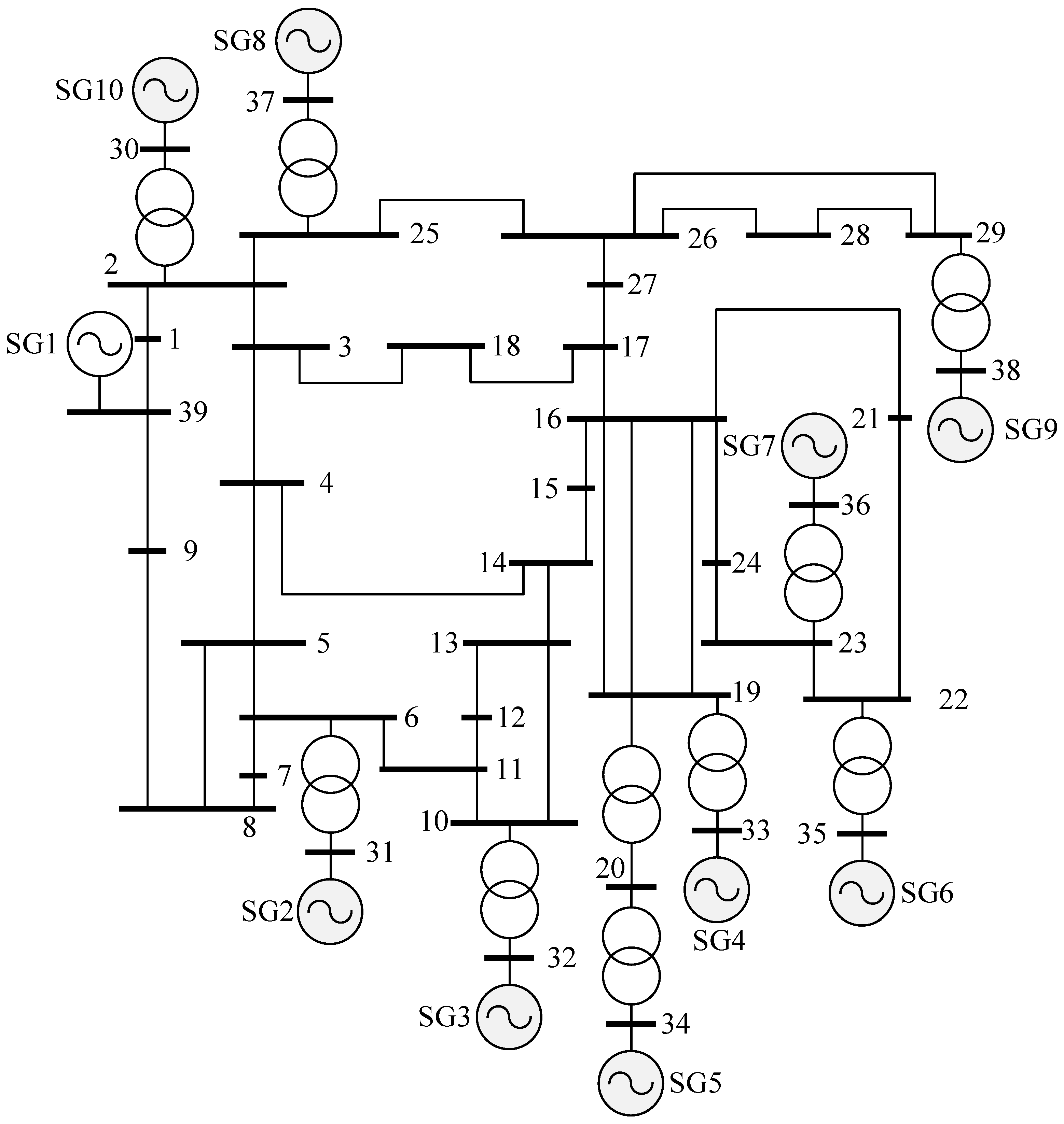
The purpose of this article is to develop and test the EC EPS methodology based on the IEEE14 [16], IEEE24 [17], and IEEE39 [18] EPS mathematical models to preserve TS and SSS, considering a classification algorithm for big data obtained from PMUs.

The scientific contribution of this paper is described as follows:

• A meta-analysis of existing EC EPS methods based on ML algorithms is presented. The advantages and disadvantages of existing methods are identified.
• A comprehensive methodology for using ML algorithms in EC EPSs is proposed.
• A study of the accuracy of EC EPS value classification based on ML algorithms is carried out.
• The feasibility of using data from synchronized vector measurement devices for use in data sampling for ML algorithms is proved.
• The feasibility of using ML algorithms to develop a flexible approach to provide SSS and TS EPSs is proved.

2. Related Works

From the ML perspective, the task of selecting CAs for EC EPSs to provide SSS and TS can be considered a multi-class classification problem. Unlike the task of estimating TS and SSS, the EC task is more complex due to the transition from binary classification [19] to multi-class. Sets of optimal CAs aimed at ensuring the stability of the post-accident regime for the accident under consideration are considered as classes. The signs for the EC EPS problem are pre-emergency values of electrical mode parameters: voltages in EPS nodes, values of active and reactive power flows across the elements of the electrical network, load angles of synchronous generators (SGs), etc. In addition, most of the considered accidents in EPSs do not require EC, i.e., the post-emergency operating mode of EPSs is stable without the use of CA. Thus, the EC EPS problem based on ML algorithms has the following features:

• A significant number of features in the data sample;
• Uneven distribution of classes in the sample (most emergency processes do not require CA implementation);
• Significant degree of overlap between classes (one CA can be part of many classes).

These features of the EC problem based on ML algorithms lead to the need for the pre-processing of data samples through the following actions:

• Reducing the dimension of the problem by reducing the number of features;
• Balancing the distribution of classes in the original data set;
• Removing outliers from the original data set.

A similar algorithm is described in [20]. In addition to processing the initial data sample, for the EC EPS task based on ML algorithms, an important step is the collection and retraining of the model in response to changes in the protected energy region (construction or dismantling of electrical network elements, active power sources, changes in SG excitation controller algorithms, etc.).

To solve the EC EPS problem based on ML algorithms, the following algorithms are used:

• Decision trees (DTs) [21,22,23];
• Random forest (RF) [24];
• Support vector machines (SVMs) [25,26,27];
• Artificial neural networks (ANNs) [28,29,30,31];
• Deep learning (DL) [32,33,34,35];
• Extreme gradient boosting (XGBoost) [36,37].

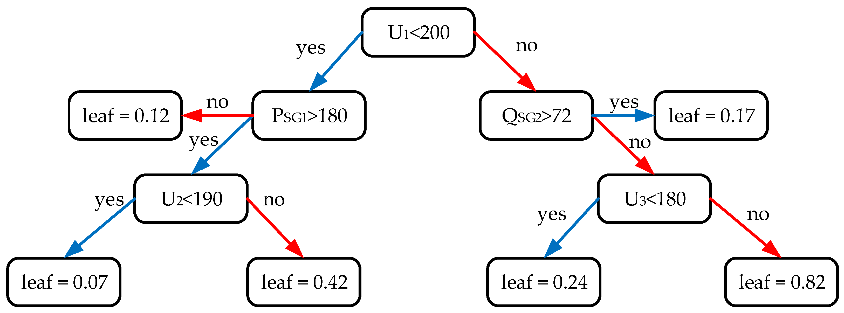
DT is a logistic classification and regression algorithm that combines logical conditions into a tree structure [38]. The DT algorithm is based on a description of data in the form of a tree-like hierarchical structure with a specific classification rule in each node, which is determined as a result of training. DT can be constructed based on the analysis of the Gini coefficient [39]:

$$\Delta G=Gini(m)-\left[\frac{n_{1m}}{n_m}Gini(m_1)+\frac{n_{2m}}{n_m}Gini(m_2)\right],$$

(1)

where Gini(m) is the value of the Gini coefficient, which shows the degree of heterogeneity of the data set m; ∆G is the value of the Gini coefficient increments after splitting the data at a node DT; n_m is the amount of data in the set m; n₁ is the amount of data in the set m₁; n₂ is the amount of data in the set m₂; m₁ and m₂ are the data after splitting set m at node DT.

As a result of DT learning, a set of rules is determined at each node in such a way as to minimize the value of the Gini coefficient. During the training process, logical rules are determined for only one sample feature in one iteration, so training data with multiple features is a time-consuming task.

In the study [21], the DT algorithm was used to determine the CA to ensure EPS stability. To reduce the time delay for algorithm training, the authors used Fisher’s linear discriminant. When forming DT, the following objective function was used:

$${\displaystyle \sum _{i_G=1}^{n_G}{k}_G}{P}_{iG}+{\displaystyle \sum _{j_L=1}^{n_L}{k}_L}{P}_{jL}\to \min ,$$

(2)

where n_G is the number of SGs by disabling which CA can be implemented, n_L is the number of loads by disabling which CA can be implemented, P_iG is the power SG i, and P_jL is the load capacity j.

The IEEE39 EPS model [22] was used to train and test the developed algorithm. The accuracy of the DT algorithm on the training set was 99.43% and on the test set—99.66%.

In [23], an algorithm for ensuring acceptable voltage levels is proposed based on the DT algorithm and data obtained from PMU devices. Testing was performed using a mathematical model from Hong Kong.

One way to overcome the disadvantages of the DT algorithm, associated with significant time costs for training and the tendency to overtrain, is to combine several shallow DT algorithms into an ensemble. This method of combining DT algorithms is called RF [40].

In the study [24], the RF algorithm was used to select CAs. The solution to the EC problem using EPS modes was divided into two stages:

• Stage 1: determination of the TS reserve for a given emergency process;
• Stage 2: CA selection using RF algorithms followed by post-emergency prediction using recurrent neural networks.

The developed algorithm was tested based on the EPS IEEE16 model.

One of the ML algorithms that allows you to solve the classification problem is SVM. This method is based on searching for separating hyperplanes that maximize the distance between classes in the data sample. When using SVM, the assumption is made that classification reliability is increased by increasing the distance between the separating hyperplanes. To construct hyper-planes, the following objective function is used [41]:

$$\frac{1}{2}{\Vert w\Vert }^2+C{\displaystyle \sum _{i=1}^N{\xi }_i}\to \min ,$$

(3)

where ||w|| is the norm of a vector perpendicular to the separating hyperplane, ξ_i are variables describing the classification error, C is a coefficient that provides a compromise between the training error and the separation boundary, and N is the number of elements in the data sample.

The authors of [25] used SVMs to analyze the static stability of EPSs based on data obtained from the PMU. The choice of SVMs is due to the ability to learn on small data samples, the absence of an obvious over-training problem, and the small number of adjustable parameters compared to ANNs. In this study, stress values at EPS nodes are used to analyze the control system. To test the proposed algorithm, the EPS IEEE39 mathematical model was used. The results of 492 simulations were used to form the data sample. The accuracy of the SVMs was 97% with a delay of 0.042 s for one emergency process.

In [26], an SVM-based algorithm for analyzing the static stability of EPSs was developed. The paper compares the classification accuracy of SVMs and ANNs on obtained data during the calculation of a series of transient processes for a mathematical model of the Brazilian power system, consisting of 2684 nodes. Using SVMs allows you to increase the accuracy by 2.5 times and reduce the time of analyzing the static stability of EPSs by 2.5 times compared to ANNs.

The authors of the study [27] proposed a method for ensuring acceptable voltage levels based on the SVM algorithm and data obtained from PMU devices. The proposed algorithm consists of two stages: training the SVM algorithm on historical data and running the trained algorithm in real time. The proposed algorithm was tested based on the EPS IEEE39 mathematical model.

The authors of [28] proposed an algorithm for analyzing SSS EPSs based on deep learning ANNs, taking into account RESs. The initial data for the algorithm are retrospective data on electricity generation from salt and wind power plants, parameters of the electrical mode of the power system, and a set of CAs for the emergency processes under consideration. The next stage is a statistical analysis of the resulting sample to reduce its dimensionality by removing features with a low correlation concerning the classification object. Next, the sample is divided into tests and training. The final stage is training the model followed by testing. The proposed algorithm was tested on the EPS IEEE68 mathematical model. The accuracy of the model was 99.89%.

The study [29] presents an EC EPS algorithm based on ANNs and the Lyapunov function, taking into account the minimization of the cost of CA implementation.

The authors of [30] used the ANN algorithm to ensure acceptable voltage levels in EPS nodes. To increase the accuracy of the ANNs, the Proximal Policy Optimization algorithm was used [31]. Testing was performed based on the EPS IEEE39 mathematical model.

In [32,33], the DL algorithm was used to develop the EC algorithm for EPS modes. This algorithm is based on the interaction of the agent function with the external environment, which is modeled as a Markov decision-making process. At each time step of the simulation, the agent can observe the state of the external environment and receive a reward signal depending on the influences issued to it. The goal of the algorithm is to apply optimal influences on the external environment to obtain the maximum total reward.

In [32], to describe the EPS as an external environment for the DL algorithm, the following system of differential-algebraic equations with restrictions is used:

$$\{\begin{array}{c}{x}_t^{\prime }=f\left(x_t,y_t,d_t,a_t\right)\\ 0=g\left(x_t,y_t,d_t,a_t\right)\\ x_t{}^{\min }\le x_t\le x_t{}^{\max }\\ y_t{}^{\min }\le y_t\le y_t{}^{\max }\\ a_t{}^{\min }\le a_t\le a_t{}^{\max }\end{array},$$

(4)

where x_t is the list of variables that determine the dynamic state of the EPS, y_t is the list of variables that determine the steady state of the EPS, a_t is the list of CAs participating in the EC operating mode of the EPS, d_t is the magnitude of the disturbance, and values with superscripts max and min denote the maximum and minimum limitation of each variable.

To train and test an algorithm that implements EC modes of EPSs based on DL, the study [32] proposed a platform containing two modules:

• Module 1 implements the DL algorithm (OpenAI Gym, Python3);
• Module 2 is used for EPS modeling and EC implementation (InterPSS, Java).

Communication between modules is ensured using the Py4J wrapper function. To configure the work of Module 1, a pre-prepared training sample is used. Next, in Module 2, the EPS transient process is simulated with the transfer of selected operating parameters to Module 1, in which the CA volume is calculated. To test the proposed platform, the standard EPS IEEE39 model was used; load shedding, generation shutdown, and the dynamic braking of generators due to braking resistors were used as CAs to ensure TS. As a result of a series of mathematical experiments, a high efficiency of the proposed platform was shown. The average CA-selection time for one emergency process was 0.18 s.

To ensure the required frequency level in isolated EPSs, the authors of [34] proposed an algorithm based on the use of DL. The proposed algorithm was tested on the EPS IEEE37 mathematical model. For the considered test scenarios, the results of calculating the accuracy of CA determination and the time delay required to analyze one emergency process are not provided. The authors argue that a promising direction for the development of the proposed algorithm is to reduce its computational complexity. Work [35] discusses the use of DL to ensure the required frequency level in isolated EPSs with RESs. The work also does not provide the results of determining the accuracy and time delays of the algorithm.

The development of the RF algorithm led to the development of the XGBoost algorithm [36], which uses gradient descent for training. Thus, it is possible to overcome the disadvantages of the RF algorithm.

The authors of the study [37] used the XGBoost algorithm to provide TS EPSs. Testing was performed on the IEEE39 EPS mathematical model, and real data were obtained from the South Carolina EPS. For the IEEE39 model, 478 stable modes and 362 unstable modes were considered, and the EC accuracy was 97.88%. For the South Carolina model, 483 stable modes and 405 unstable modes were considered, and the CA selection accuracy was 98.62%.

Table 2 provides an analysis of the reviewed ML algorithms used for EC EPSs.

Table 2. Analysis of the considered ML algorithms.

Algorithm	References	Merits	Drawbacks	Field of Applicability
DT	[21,22,23]	High reliability and representativeness of the results	Significant time costs for training the algorithm	TS
RF	[24]	A high degree of parallelism, high performance	High random access memory requirements	TS
SVM	[25,26,27]	High performance of the trained algorithm	Instability when working with noisy data	SSS
ANN	[28,29,30,31]	Resistant to data noise, significant fault tolerance	Tendency to overtrain	SSS
DL	[32,33,34,35]	Does not require a significant amount of training samples	It is possible to select optimal CAs due to the limited actions of the agent	TS
XGBoost	[36,37]	The high speed of the trained algorithm	Difficulty in determining hyperparameters	TS

The considered ML algorithms used to select a CA for storing TS EPSs are characterized by several disadvantages associated with the suboptimal choice of CAs, significant time costs for training the model, high requirements for RAM, a tendency to overtrain, and the complexity of determining hyperparameters. The XGBoost algorithm has the shortest CA-selection time to store TS EPSs compared to the DL and DT algorithms. For the RF algorithm, the study does not provide an estimate of time costs. To analyze and store SSS EPSs, two machine learning algorithms were considered: SVMs and ANNs. The highest performance of CA selection was shown for the SVM algorithm. The main disadvantage of this algorithm is its sensitivity to outliers and noise in the source data, which can lead to a significant displacement of the separating hyperplane from the optimal position. This problem can be effectively solved through the use of statistical filters at the data pre-processing stage.

One of the significant disadvantages of the considered ML algorithms is their non-universality in terms of choosing a CA only for storing TS or SSS. In addition, for the considered algorithms to work, a pre-generated list of accidents is required, for which the selection of a CA is required. This approach significantly reduces the adaptability of EC EPSs.

The purpose of this study is to develop and test, on mathematical data, a universal CA-selection algorithm for saving TS and SSS EPSs based on big data analysis through the use of DL algorithms. The following algorithms are under consideration: recurrent neural networks (RNNs), long short-term memory networks (LSTMs), restricted Boltzmann machines (RBMs), and self-organizing maps (SOMs). The selection of these algorithms was based on the analysis of the study [42].

The scientific novelty of this research lies in solving the problem of adaptive EC EPSs based on deep learning methods for preserving TS and SSS. The adaptability of the proposed method is ensured by the absence of the need to specify a list of accidents under consideration for which the CA is selected. To increase the accuracy of CA selection in the original data set, measurements obtained from the PMU are used.

3. Description of the EPS EC Technique Based on the ML Algorithm

For the EC EPS algorithm, the block diagram shown in Figure 1 is used.

Figure 1. Flowchart of the EC EPS algorithm.

The first step in the flowchart shown in Figure 1 is data generation. To form a data sample, two sources can be used: the results of mathematical modeling and real data obtained during the registration of transient processes in real EPSs. The next stage is the selection of features to increase the speed of training procedures for the DL model. After training, the DL model is tested, and the classification quality criteria are analyzed. If the classification quality is unacceptable, the DL model is retrained with the correction of hyperparameters or a set of features. Once an acceptable classification quality is achieved, the trained DL model is integrated into the EC EPS process, which runs in real time. When there is a change in the EPS structure [43], the DL model is retrained. The following is a detailed description of each of the stages of the flowchart shown in Figure 1.

3.1. Data Generation

The results of mathematical modeling of transient processes can be used as data for sampling, indicating the selected CA for storing TS or SSS. This modeling is most often performed using software packages for calculating transient processes in EPSs [44]. The main advantage of this method of obtaining data for sampling is the ability to simulate a wide range of transient processes with different electrical network configurations and different types of accidents. The main disadvantage of this method of obtaining data is the possible error in modeling transient processes in EPSs. The occurrence of error is associated with the use of irrelevant parameters of EPS mathematical models, regulators, and control devices. The second source of data is records of real transient processes occurring in the EPS. The registration of accidents can be performed using PMUs [45], which makes it possible to obtain a description of transient processes with high accuracy. The main disadvantage of this source of information is related to the difficulty of obtaining data because a loss of stability accident is a rare event [46]. Therefore, a data sample can be generated by combining real and simulated data. If there are changes in the EPS structure, the data sample must be replaced, because adding or removing elements from the EPS block diagram almost completely changes the nature of the transient processes. The data selection should be updated when there are changes in the EPS structure (implementation of new SGs and transmission lines) or when there are new records of accidents occurring in the EPS.

In this study, numerical modeling performed in the MATLAB/Simulink environment was used to generate a data sample. The standard mathematical models EPS IEEE14 [16], IEEE24 [17], and IEEE39 [18] with modified load values and SG powers were used. A detailed description of the mathematical models used is given in Appendix A, Appendix B, and Appendix C. To select CAs, an algorithm adapted for the analysis of TS and SSS from the study [47] was used. To simulate a series of transient processes, a proportional change in loads and generations was performed in the EPS models used.

After generating the initial data sample, it must be processed to remove outliers, noise, and features with a high correlation.

3.2. Feature Selection

Feature selection is an important step in preparing a data sample before training an ML algorithm. Feature selection is performed to reduce the dimensionality of the CA selection problem being solved and to reduce the model training time. The selection of features is carried out according to the stages described in Figure 2.

Figure 2. Flowchart of feature selection algorithm.

Thus, a three-step procedure combining the Spearman correlation coefficient analysis and the use of the RF algorithm [48] is used for feature selection. The Spearman correlation coefficient is calculated using the following equation:

$$\rho =1-\frac{6{\displaystyle \int d^2}}{n\left(n^2-1\right)},$$

(5)

where ρ is the Spearman correlation value, d is the difference in ranks for pair (X, Y) of two series of numbers, and n is the length of rows X and Y.

3.3. Description of the DL Algorithms Used

This study considers four DL algorithms: RNNs, LSTMs, RBMs, and SOMs. Below are the basic operating principles of each algorithm. To train and use DL algorithms, the Python3 programming language was used in conjunction with the TensorFlow, Keras, scikit-learn, and sklearn_som libraries.

3.3.1. RNNs

The RNN algorithm is based on ANNs, in which the connections between layers are a directed sequence [49]. The calculations required at each step in an RNN are defined by the following equations:

$$\{\begin{array}{c}{h}^{(t)}=\sigma \left(W^{hx}{x}^{(t)}+W^{hh}{h}^{(t-1)}+b_h\right)\\ y^{(t)}=\mathrm{softmax}\left(W^{yh}{h}^{(t)}+b_y\right)\end{array},$$

(6)

where h^(t) is the value in the hidden node at time t, h^(t−1) is the value in the hidden node at time t − 1, x^(t) is the value of input data at time t, y^(t) is the output value at time t, W^hx is the weight matrix between the input and hidden layers, W^hh is the matrix of weight coefficients between hidden layers, W^yh is the matrix of weighting coefficients between the input and output, b_h is the hidden layer offset vector, b_y is the displacement vector of the output layer, softmax() is the multivariate logistic function, and σ is the activation function.

3.3.2. LSTMs

The architecture of LSTMs is similar to that of RNNs. The difference is that an LSTM replaces hidden layers with a memory cell. Each memory cell contains a node with a self-connected recurrent edge of a certain weight [50]. The calculations in LSTMs are defined by the following equations:

$$\{\begin{array}{c}{f}_t={\sigma }_g\left(W_f{x}_t+U_f{h}_{t-1}+b_f\right)\\ i_t={\sigma }_g\left(W_i{x}_t+U_i{h}_{t-1}+b_i\right)\\ o_t={\sigma }_g\left(W_o{x}_t+U_o{h}_{t-1}+b_o\right)\\ C_t={\sigma }_c\left(W_c{x}_t+U_c{h}_{t-1}+b_c\right)\\ c_t=f_t\odot c_{t-1}+i_t\odot C_t\\ h_t=o_t\odot {\sigma }_h\left(c_t\right)\end{array},$$

(7)

where x_t is the input vector; h_t is the output vector, c_t is the state vector; W, U, and b are the matrices and vector of model parameters; f_t, f_i, and o_t are the gate’s activation vector; σ_g is the sigmoid-based activation function; σ_c and σ_h are the activation function based on hyperbolic tangent; and ⊙ is the Hadamard product operator.

3.3.3. RBMs

An RBM is a type of generative stochastic ANN in which neurons are divided into visible and hidden layers and connections are only allowed between neurons of different types, thus limiting connections [51]. For RBMs, there is a concept of network energy through which all calculations are performed:

$$E\left(u,h\right)=-a^{T}u-b^{T}h-u^{T}Wh,$$

(8)

where E is the network energy value, a is the displacement vector for the visible layer, b is the displacement vector for the hidden layer, W is the weight matrix, u is the binary elements of the visible layer, h is the hidden layer’s binary elements, and T is the denotation of the transposition operation.

3.3.4. SOMs

An SOM is a type of ANN. The main difference between this technology and neural networks trained using the backpropagation algorithm is that the training method uses an unsupervised learning method, that is, the learning result depends only on the structure of the input data [52]. The SOM operation algorithm can be presented as follows:

• Initialization;
• Selecting a vector from a data set;
• Finding the best matching unit for the selected vector;
• Determination of the number of best matching units (BMUs);
• Definition of error.

3.4. Algorithm Quality Assessment

To assess the classification quality of the trained algorithm, the following parameters were used: accuracy (ACC), missed detection rate (MDR), false alarm rate (FAR), and area under the receiver operating characteristic curve (AUC). The parameters ACC, MDR, and FAR are expressed through the values true positive (TP), true negative (TN), false positive (FP), and false negative (FN) [53].

ACC is a coefficient that determines the ratio of correctly classified data to the total number of classifications:

$$ACC=\frac{TP+TN}{TP+TN+FP+FN}\cdot 100\%.$$

(9)

MDR is a ratio that determines the ratio of examples that were classified as false positives to the total number of classifications:

$$MDR=\frac{FP}{TP+TN+FP+FN}\cdot 100\%.$$

(10)

FAR is a ratio that determines the ratio of examples that were classified as false negatives to the total number of classifications:

$$FAR=\frac{FN}{TP+TN+FP+FN}\cdot 100\%.$$

(11)

AUC is a value that determines the area under the receiver operating characteristic curve. The AUC metric is used for binary classifications. In multivariate classifications, AUC can be used for only two classes [54].

3.5. Real-Time Application

In this study, the real-time EC problem is considered only theoretically and is a direction for future research. A block diagram describing the use of the proposed EC algorithm based on ML and data received from the PMU is shown in Figure 3. When an accident occurs (in Figure 3, the accident location is shown with a red arrow), PMU devices register emergency currents and voltages with transmission (in Figure 3, the process of transmitting information from the PMU to the data center is shown by blue arrows) to the data center, which has EC command transmission channels (in Figure 3, the process of transmitting a command to implement CAs is shown by green arrows) to turn off SGs and loads in a protected energy region. Based on the obtained values of current and voltage synchrophasors, the trained DL algorithm selects CAs in the form of a set of switchable SGs and loads. Next, the set of CAs is transmitted via communication channels to control objects.

Figure 3. Flowchart of real-time EC EPS algorithm’s application.

To implement this EC principle, it is necessary to estimate the acceptable time delay between the transfer of current and voltage synchrophasors to the data center and the implementation of CAs at power system facilities. This problem can be solved using real-time EPS transient simulations [55,56,57,58,59,60].

4. Case Study

For numerical experiments, MATLAB/Simulink was used to simulate transient processes, and Python3 was used to train and analyze DL algorithms.

4.1. Data Preparation

To generate data samples for the IEEE14, IEEE24, and IEEE39 models, cyclic calculations of transient processes with CA selection were used. During the cyclic calculations, the following model parameters were changed: loads in nodes, values of active- and reactive-power SGs, and the topology was changed taking into account single repairs of network elements. When considering repairs of network equipment, situations of isolating isolated islands were excluded [61]. To generate the data and CA selection, the following perturbations were considered [47]:

• Three-phase short circuits of 0.1 and 0.2 s durations;
• Two-phase short-circuits of 0.1, 0.2 and 0.3 s durations;
• Single-phase short circuits of 0.1, 0.2, 0.3, and 0.4 s durations;
• Disconnection of the transmission line;
• SG switching off.

Short circuits were considered for selecting CAs to preserve TS. Transmission lines and SG disconnections were considered for selecting CAs to preserve SSS. The transient calculations in the considered EPS mathematical models were performed in MATLAB/Simulink. CA selection was performed by transferring the initial data to a dynamic library implementing CA-selection algorithms.

The following features were considered in the data sample: voltages in nodes, voltage phases in nodes, current loads of electrical network elements, active power flows, reactive power flows, active power SGs, reactive power SGs, and load angle SGs. Table 3 shows the characteristics of the obtained initial data samples: the number of features, the total volume of the data sample, the number of scenarios with CAs, the number of scenarios without CAs, and the degree of class imbalance. A scenario is understood as the result of calculating the transient process for the considered accident. Figure 4 provides a graphical representation of class imbalance in the original data samples. The abscissa axis of Figure 4 shows the names of the considered EPS mathematical models.

Table 3. Parameters of initial data samples.

Model	Number of Features	Total Data Sample Size	Number of Scenarios with CAs	Number of Scenarios without CAs	ID, %
IEEE14	107	3465	692	2772	19.9
IEEE24	244	23,940	6548	16,758	27.3
IEEE39	313	43,470	13,546	30,429	31.1

Figure 4. Imbalance of classes of the original data samples.

The degree of class imbalance (ID) [62] is calculated using the following equation:

$$ID=\frac{N_{CA}}{N_s}\cdot 100\%,$$

(12)

where ID is the degree of class imbalance, N_CA is the number of scenarios with CAs, and N_S is the total number of scenarios considered.

The volume of the initial sample for each model is determined by the following equation [19]:

$$N_{DS}=N_{SG}\cdot N_R\cdot N_L\cdot N_V,$$

(13)

where N_DS is the initial data sample volume, N_R is the number of repairs being considered, N_L is the number of nodes with variable loads, N_SG is the number of SGs with variable active powers, and N_V is the coefficient characterizing the number of changes in loads and generations during modeling.

In addition to the imbalance of data for classes with and without CAs in the selection of data, there is an imbalance of classes describing the composition of CAs, which must be applied to maintain the stability of EPSs. Therefore, for the initial data sample, it is necessary to ensure equality between classes with and without CAs, as well as equality between classes with different sets of CAs. For this purpose, a data sample-thinning procedure is used to ensure class balance.

Table 4 shows the results of class balancing in the original data set. Figure 5 shows a graphical representation of the class imbalance in the processed data sample.

Table 4. Parameters of processed data samples.

Model	Number of Features	Total Data Sample Size	Number of Scenarios with CAs	Number of Scenarios without CAs	ID, %
IEEE14	107	1386	749	637	54.0
IEEE24	244	8618	4412	4206	51.1
IEEE39	313	14,779	8172	6607	55.3

Figure 5. Imbalance of classes of processed data samples.

After ensuring the balance of the data sample, feature selection is performed using the algorithm described in Figure 2. The first stage of this algorithm is the removal of features with a low correlation concerning the answer. Table 5 shows the results of removing features that have Spearman correlation values concerning the answer below 0.3.

Table 5. The result of removing features with a low correlation to the target.

Model	The Initial Number of Features	Number of Features Removed	Number of Features after Processing	Removed Features
IEEE14	107	31	76	Values of current loads of network elements; voltages in nodes 14, 11, and 10; reactive powers along lines adjacent to nodes 9 and 5
IEEE24	244	42	202	Values of current loads of network elements; voltages in nodes 6, 14, 19, and 20
IEEE39	313	54	259	Values of current loads of network elements; voltages in nodes 3, 4, 7, 11–14, and 24

The low correlation value of current loads of electrical network elements to the CA class, aimed at preserving TS and SSS, is explained by the nature of the phenomenon of EPS instability [63,64,65]. The preservation of TS and SSS largely depends on the flow of active power and voltage levels; there is practically no direct connection with the current loads of the elements of the electrical network. There is only an indirect connection through the magnitude of the loading currents of the electrical network and voltage loss. Also, the low correlation concerning CA class corresponds to node voltages electrically distant from SGs. Including highly cross-correlated features in the training set can lead to poor task conditioning and can lead to instability and unreliability in determining the optimal hyperparameters of the DL model [66]. Table 6 shows the results of removing features that have Spearman cross-correlation values higher than 0.9.

Table 6. The result of removing features with high cross-correlations.

Model	The Initial Number of Features	Number of Features Removed	Number of Features after Processing	Removed Features
IEEE14	76	2	74	Node voltages 12 and 13
IEEE24	202	1	201	Node voltage 5
IEEE39	259	3	256	Node voltages 18, 27, and 28

In the data sample, a Spearman correlation value higher than 0.9 was obtained for the voltages of some nodes. Such cases correspond to the low electrical distance between EPS nodes. As a result of the analysis of the cross-correlation of features, two features were removed from the sample corresponding to the IEEE14 model, one feature was removed from the sample corresponding to the IEEE24 model, and three features were removed from the sample corresponding to the IEEE39 model. The next stage of processing the data sample is to analyze the importance of features for the RF algorithm. The RF algorithm allows you to obtain the importance values of each feature during classification. The RF algorithm was trained by dividing the data sample into two parts: training and testing. Table 7 shows the values of hyperparameters obtained during the training of the RF algorithm. To obtain optimal hyperparameters, the standard random search procedure was used [67].

Table 7. Values of the RF algorithm hyperparameters.

Model	n_Estimators	Max_Features	Max_Depth	Min_Samples_Split	Min_Samples_Leaf
IEEE14	112	2	3	10	8
IEEE24	214	7	6	12	9
IEEE39	287	9	5	30	16

Table 7 uses the following notation: n_estimators are the number of decision trees in the ensemble, max_features are the maximum number of features considered for splitting a node, max_depth is the maximum number of levels of the decision tree, min_samples_split is the minimum amount of data placed in a node before splitting, and min_samples_leaf is the minimum amount of data placed in a leaf node. Figure 5 shows an example of one of the decision trees for the IEEE14 model. In Figure 6, the following notations are used: U₁ is the voltage in node 1, U₂ is the voltage in node 2, U₃ is the voltage in node 3, P_SG1 is the active power of the first SG, Q_SG2 is the reactive power of the second SG, and leaf is the value in the leaf node. Table 8 shows the results of removing features with an importance of less than 0.2. For the RF algorithm, the minimum significance corresponds to the reactive power flows indicated in Table 8. Figure 7 shows the process of changing the number of features in the processing of a data sample. The abscissa axis indicates the stage of processing the data sample, as described in Figure 2. Step 0 shows the initial value of the features in the data sample.

Figure 6. One of the decision trees for the IEEE14 model.

Table 8. The result of removing features after decision trees analyses.

Model	The Initial Number of Features	Number of Features Removed	Number of Features after Processing	Removed Features
IEEE14	74	5	69	Flows of reactive power along branches extending from node 4
IEEE24	201	12	189	Flows of reactive power along branches extending from nodes 8, 13, 17, and 21
IEEE39	256	18	238	Flows of reactive power along branches extending from nodes 16, 19, 26, and 28

Figure 7. Changes in features during the processing of data samples: (a) IEEE14 model; (b) IEEE24 model; (c) IEEE39 model.

During the processing of the initial data sample, the balance of the sample by class was ensured and features were selected using the methods of statistical analysis and analysis of the importance of features for the RF algorithm.

4.2. Training and Testing Algorithms without Taking into Account PMU Data

After preparing the data sample, the stages of training and testing the algorithms were completed: RNNs, LSTMs, RBMs, and SOMs. The algorithms were trained using the standard algorithm exhaustive grid search from the TensorFlow, Keras, scikit-learn, and sklearn_som libraries. Table 9, Table 10, Table 11 and Table 12 show the main defined hyperparameters of the algorithms. In Table 9, Table 10, Table 11 and Table 12, the following notations are used: RNN_Size is the size of the hidden layer of the RNN, RNN_Layers is the number of layers in the RNN, Sequence_Length is the size of the data packet, Batch_Size is the length of the sequence for the RNN, Epoch_Number is the number of epochs (one pass forward and backward for the training example), Act_Func is the activation function, LSM_Layer is the number of layers in the LSM, Weight_Initializer is the method of setting initial weights, glorot_uniform is the glorot uniform initializer [68], Dropout_Ratio is the regularization coefficient of the DL model, tanh is the hyperbolic tangent, Relu is the rectified linear unit, Kernel_size is the kernel size, Hidden_Number is the number of nodes in the hidden-feature layer, PrimaryCaps_Number is the number of nodes in the PrimaryCaps layer, N_function is the Neighborhood Distance Function, Gaussian_width is the width of the Gaussian function used, Learning_Rate is the learning rate, and BMU_Selection is the method for determining the BMU.

Table 9. Values of hyperparameters of the RNN algorithm.

Model	RNN_Size	RNN_Layers	Sequence_Length	Batch_Size	Epoch_Number
IEEE14	256	2	25	50	250
IEEE24	256	3	28	55	250
IEEE39	256	5	28	70	250

Table 10. Values of hyperparameters of the LSTM algorithm.

Model	Act_Func	LSM_Layer	Epoch_Number	Weight_Initializer	Dropout_Ratio
IEEE14	tanh	100	250	glorot_uniform	0.1
IEEE24	tanh	100	250	glorot_uniform	0.2
IEEE39	tanh	150	250	glorot_uniform	0.2

Table 11. Values of hyperparameters of the RBM algorithm.

Model	Act_Func	Epoch_Number	Kernel_Size	Hidden_Number	PrimaryCaps_Number
IEEE14	Relu	250	10	128	64
IEEE24	Relu	250	10	128	64
IEEE39	Relu	250	24	128	64

Table 12. Values of hyperparameters of the SOM algorithm.

Model	Kernel_Size	N_Function	Gaussian_Width	Learning_Rate	BMU_Selection
IEEE14	70	Gaussian	7	0.04	Euclidean distance
IEEE24	150	Gaussian	12	0.03	Euclidean distance
IEEE39	210	Gaussian	22	0.01	Euclidean distance

To train the model, an ACC threshold value of 95% was chosen [69,70]. When this value is reached, the training process stops to prevent overtraining of the DL model. The ACC threshold value can be selected depending on the requirements of the problem being solved and changed during the operation of the trained DL algorithm.

Figure 8 shows the changes in ACC depending on the training iteration. Graphs of changes in ACC for the various considered models (IEEE14, IEEE24, and IEEE39) and for the various algorithms (RNNs, LSTMs, RBMs, SOMs) are presented. The red dotted line shows the ACC threshold value of 95%.

Figure 8. Change in ACC indicator during training of DL models without taking into account data from PMU: (a) model IEEE14, RNN algorithm; (b) model IEEE24, RNN algorithm; (c) model IEEE39, RNN algorithm; (d) model IEEE14, LSTM algorithm; (e) model IEEE24, LSTM algorithm; (f) model IEEE39, LSTM algorithm; (g) model IEEE14, RBM algorithm; (h) model IEEE24, RBM algorithm; (i) model IEEE39, RBM algorithm; (j) model IEEE14, SOM algorithm; (k) model IEEE24, SOM algorithm; (l) model IEEE39, SOM algorithm.

For training and testing, a procedure was performed to divide the sample into test and training. A total of 80% of the original sample was selected for training and 20% for testing [71].

Table 13 shows the results of the trained DL algorithms on the test data.

Table 13. Analysis of the results of DL algorithms on test data samples.

Model	Parameter	Algorithm
		RNN	LSTM	RBM	SOM
IEEE14	MDR, %	1.11	1.38	1.67	1.73
	FAR, %	1.43	1.65	1.34	1.29
	ACC, %	93.87	94.63	94.15	92.29
	AUC	0.97	0.95	0.95	0.94
IEEE24	MDR, %	2.11	1.87	1.61	1.93
	FAR, %	2.25	2.15	2.36	1.81
	ACC, %	93.83	94.85	93.84	92.17
	AUC	0.97	0.96	0.98	0.97
IEEE39	MDR, %	2.52	1.86	1.68	1.59
	FAR, %	2.10	1.80	1.65	1.16
	ACC, %	92.25	93.44	92.74	91.90
	AUC	0.97	0.98	0.95	0.96

From the results of testing DL algorithms, it is clear that with an increasing dimension of the EPS model, the accuracy of CA selection decreases, which can be explained by an increase in uncertainty due to the significant complexity of considering the entire list of accidents. It is also clear that the best classification results correspond to the LSTM algorithm and the worst results correspond to the SOM algorithm. In this section, DL algorithms were trained and tested without data from the PMU [72], i.e., there were no voltage phases in the data sample.

4.3. Testing Algorithms by Taking into Account PMU Data

Table 14, Table 15, Table 16 and Table 17 show the main defined hyperparameters of the algorithms, taking into account the data received from the PMU.

Table 14. Values of hyperparameters of the RNN algorithm taking into account PMU data.

Model	RNN_Size	RNN_Layers	Sequence_Length	Batch_Size	Epoch_Number
IEEE14	256	2	23	48	250
IEEE24	256	3	26	51	250
IEEE39	256	5	28	65	250

Table 15. Values of hyperparameters of the LSTM algorithm taking into account PMU data.

Model	Act_Func	LSM_Layer	Epoch_Number	Weight_Initializer	Dropout_Ratio
IEEE14	tanh	90	250	glorot_uniform	0.1
IEEE24	tanh	120	250	glorot_uniform	0.2
IEEE39	tanh	136	250	glorot_uniform	0.2

Table 16. Values of hyperparameters of the RBM algorithm taking into account PMU data.

Model	Act_Func	Epoch_Number	Kernel_Size	Hidden_Number	PrimaryCaps_Number
IEEE14	Relu	250	8	128	64
IEEE24	Relu	250	8	128	64
IEEE39	Relu	250	20	128	64

Table 17. Values of hyperparameters of the SOM algorithm taking into account PMU data.

Model	Kernel_Size	N_Function	Gaussian_Width	Learning_Rate	BMU_Selection
IEEE14	60	Gaussian	6	0.04	Euclidean distance
IEEE24	120	Gaussian	10	0.03	Euclidean distance
IEEE39	200	Gaussian	22	0.01	Euclidean distance

To train the model, an ACC threshold value of 95% was chosen [69,70]. When this value is reached, the training process stops to prevent overtraining of the DL model. Figure 9 shows changes in ACC depending on the training iteration. Table 18 shows the results of the trained DL algorithms on the test data.

Figure 9. Change in ACC indicator during the training of DL models with taking into account data from PMU: (a) model IEEE14, RNN algorithm; (b) model IEEE24, RNN algorithm; (c) model IEEE39, RNN algorithm; (d) model IEEE14, LSTM algorithm; (e) model IEEE24, LSTM algorithm; (f) model IEEE39, LSTM algorithm; (g) model IEEE14, RBM algorithm; (h) model IEEE24, algorithm RBM; (i) model IEEE39, RBM algorithm; (j) model IEEE14, SOM algorithm; (k) model IEEE24, SOM algorithm; (l) model IEEE39, SOM algorithm.

Table 18. Analysis of the results of DL algorithms on test data samples, taking into account data from the PMU.

Model	Parameter	Algorithm
		RNN	LSTM	RBM	SOM
IEEE14	MDR, %	1.08	1.36	1.62	1.72
	FAR, %	1.43	1.61	1.33	1.21
	ACC, %	93.72	94.83	94.17	92.31
	AUC	0.96	0.92	0.95	0.92
IEEE24	MDR, %	2.08	1.83	1.60	1.92
	FAR, %	2.12	2.12	2.31	1.80
	ACC, %	93.65	94.88	93.86	92.14
	AUC	0.92	0.94	0.90	0.91
IEEE39	MDR, %	2.50	1.84	1.61	1.58
	FAR, %	2.07	1.72	1.60	1.14
	ACC, %	92.18	93.64	92.76	91.91
	AUC	0.98	0.97	0.93	0.96

Taking into account the phases of the voltages of the nodes considered by the EPS leads to an increase in the accuracy of the CA classification. This fact is explained by the high degree of dependence of SSS and TS on active power flows, which are determined by the distribution of voltage phases across EPS nodes. The best classification results correspond to the LSTM algorithm.

4.4. Testing the Ability to Determine a Set of CA for an Accident That Is Not in the Data Sample

To test the ability of DL algorithms to independently generate an optimal set of CAs for a given set of characteristics, a calculation of the transient process was performed with an accident not taken into account in the initial data sample, which consists of a three-phase short circuit in node 9 of the IEEE14 model. An LSTM algorithm is used to select CAs. Figure 10 shows the angular speeds of SGs without introducing CAs. In the IEEE14 model, SG1 is balancing, so its load angle is not shown in Figure 10. Figure 11 shows the angular speeds of SGs with the introduction of CAs.

Figure 10. Changing the angular speeds of SG2, SG3, SG6, and SG8 during a short circuit in node 9 without implementing CAs.

Figure 11. Change in angular speeds of SG2, SG3, SG6, and SG8 during a short circuit in node 9 with CA implementation.

The loss of TS on the graph of angular speed SGs is indicated by an excess of 1 p.u. [73]. Figure 10 shows the process of losing the TS EPS, highlighting two groups of generators: SG3, SG8, SG2, and SG6. As a result of using the LSTM algorithm, the CA was selected in the form of disabling SG8 to preserve the TS EPS.

4.5. Comparison of Accuracy of DL Algorithms with DT, RF, SVM, and XGBoost Algorithms

The DT, RF, SVM, XGBoost, and DL algorithms’ RNNs, LSTMs, RBMs, and SOMs were selected to perform the comparison of the CA EPS value classification results. The comparison of the performance of the algorithms was executed on the data obtained for the IEEE39 mathematical model. The hyperparameters of the DT, RF, SVM, and XGBoost algorithms were determined using the standard exhaustive grid search approach.

Table 19 shows the obtained values of the hyperparameters of the DT, RF, SVM, and XGBoost algorithms.

Table 19. Values of hyperparameters of the DT, RF, SVM, and XGBoost algorithms.

Algorithm	Hyperparameters
DT	criterion = “gini”
	splitter = “best”
	max_depth = 10
	min_samples_split = 2
RF	n_estimators = 25
	max_depth = 3
	min_samples_split = 0.01
	min_samples_leaf = 0.01
	max_features = 7
SVM	degree = 3
	gamma = 1
	kernel = Radial Basis Function
XGBoost	alpha = 0.05
	lambda = 0.05
	gamma = 1
	max_depth = 5
	base_score = 0.6
	n_estimators = 35
	learning_rate = 1
	max_delta_step = 1

Table 19 assumes the following notations: criterion is the function for measuring the quality of splitting the DT data sample, splitter is a strategy used for splitting at each DT node, max_depth is the maximum DT depth, min_samples_split is the minimum number of samples needed to split the inner DT node, n_estimators is the number of DTs in the RF, min_samples_leaf is the minimum number of samples needed to be in the leaf node, max_features is the number of features needed to be considered when searching for the best separation, degree is the degree of the polynomial kernel function, gamma is the kernel coefficient, kernel is the kernel type, alpha is the L1 regularization factor, lambda is the L2 regularization factor, gamma is the minimum loss reduction factor required for node separation, learning_rate is the learning rate, base_score is the initial prediction score, and max_delta_step is the maximum delta step.

Table 20 shows the values of the ACC ratio determined by expression (9).

Table 20. Average values of ACC ratio for the considered algorithms.

Algorithm	ACC, %
Without PMU data
RNN	92.25
LSTM	93.44
RBM	92.74
SOM	91.90
DT	62.17
RF	71.85
SVM	70.13
XGBoost	80.66
With PMU data
RNN	92.18
LSTM	93.64
RBM	92.76
SOM	91.91
DT	72.54
RF	77.12
SVM	75.43
XGBoost	81.57

Due to the significant number of features in the data set and the high share of hidden patterns described by the system of algebraic-differential equations of the dynamic state of EPSs, the accuracy of the DT, RF, SVM, and XGBoost algorithms is 18.6% lower than for the RNN, LSTM, RBM, and SOM algorithms in the average.

Based on both Table 13 and Table 18, the highest accuracy of the CA EPS classification corresponds to the LSTM algorithm.

5. Conclusions

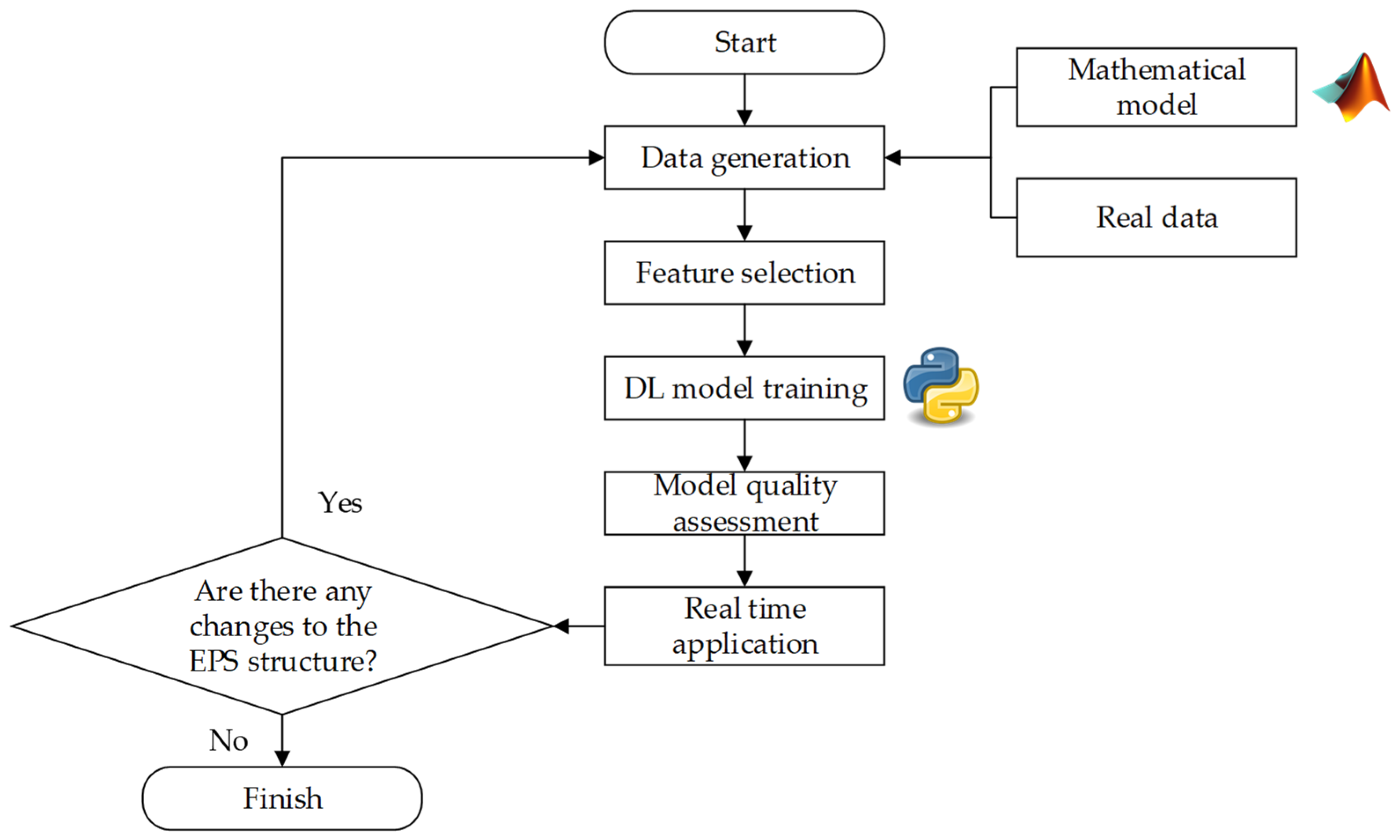
This study presents the results of developing an EC EPS methodology based on DL algorithms and obtained data from PMUs. Due to the introduction of a significant number of RESs and the rules tightening the functioning of the electricity market, there are significant changes in the speed of transition processes for modern EPSs. Therefore, traditional EC EPS systems do not meet the requirements for speed and reliability. This paper proposes a methodology for selecting a CA for storing TS and SSS EPSs.

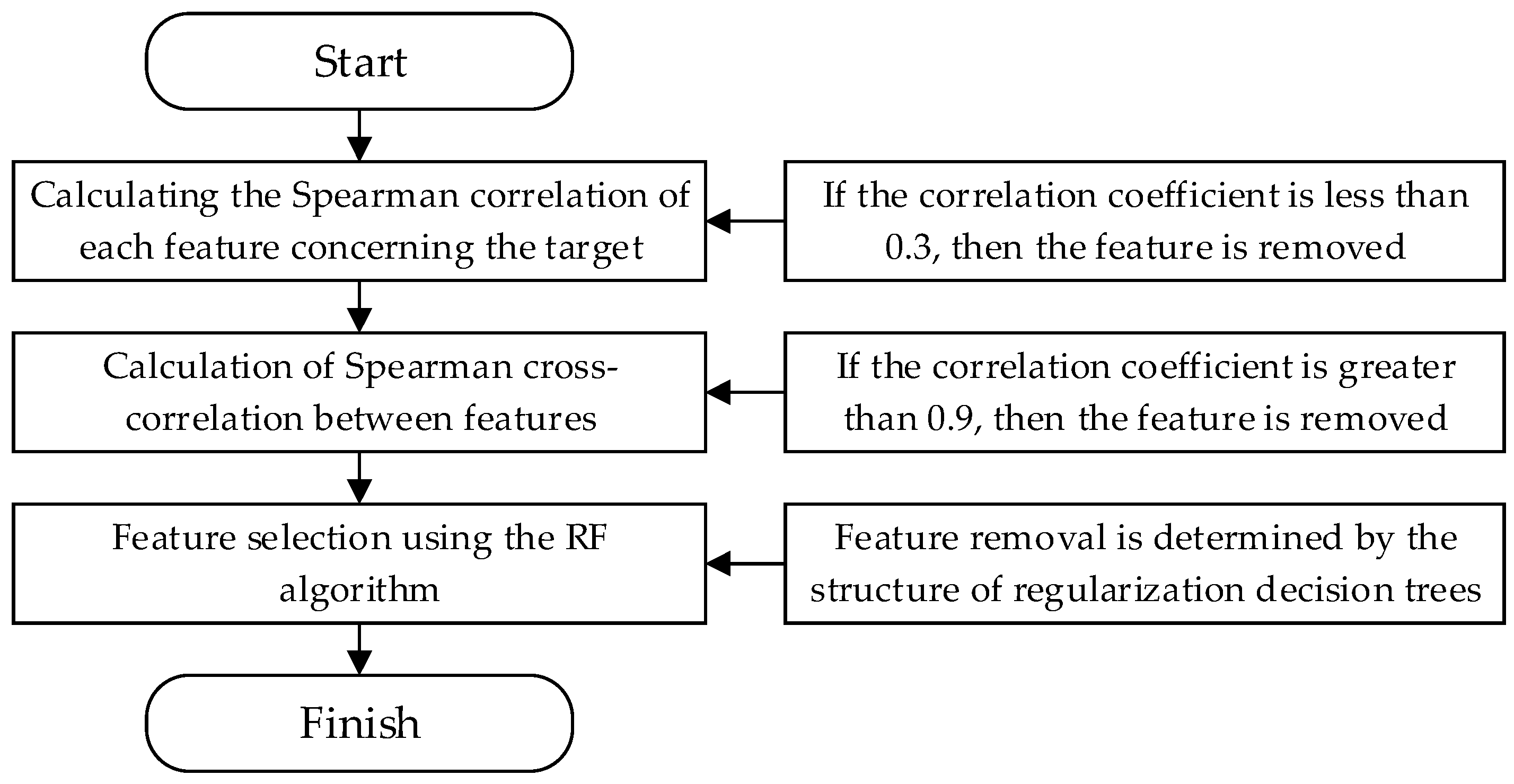
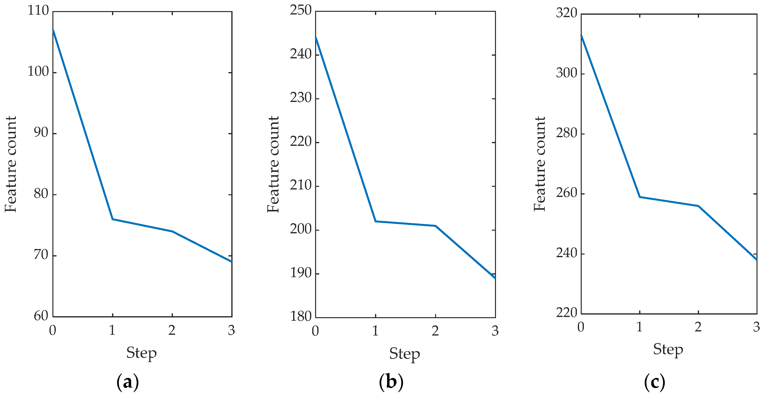
The following DL algorithms were considered: RNNs, LSTMs, RBMs, and SOMs. To form a data sample, the following EPS mathematical models were used: EEE14, IEEE24, and IEEE39. To process the data sample, a three-step algorithm was used, which consists of a sequential analysis of the Spearman correlation coefficient of each characteristic from the responses, the cross-Spearman correlation coefficient of the characteristics, and an analysis of the importance of the characteristics for the RF algorithm. For the IEEE14 model, the initial number of features in the data set was 107, for the IEEE24 model it was 244, and for the IEEE39 model, it was 313. After applying the feature selection algorithm shown in Figure 2, the number of features was reduced for IEEE14 to 69, for IEEE24 to 189, and for IEEE39 to 238.

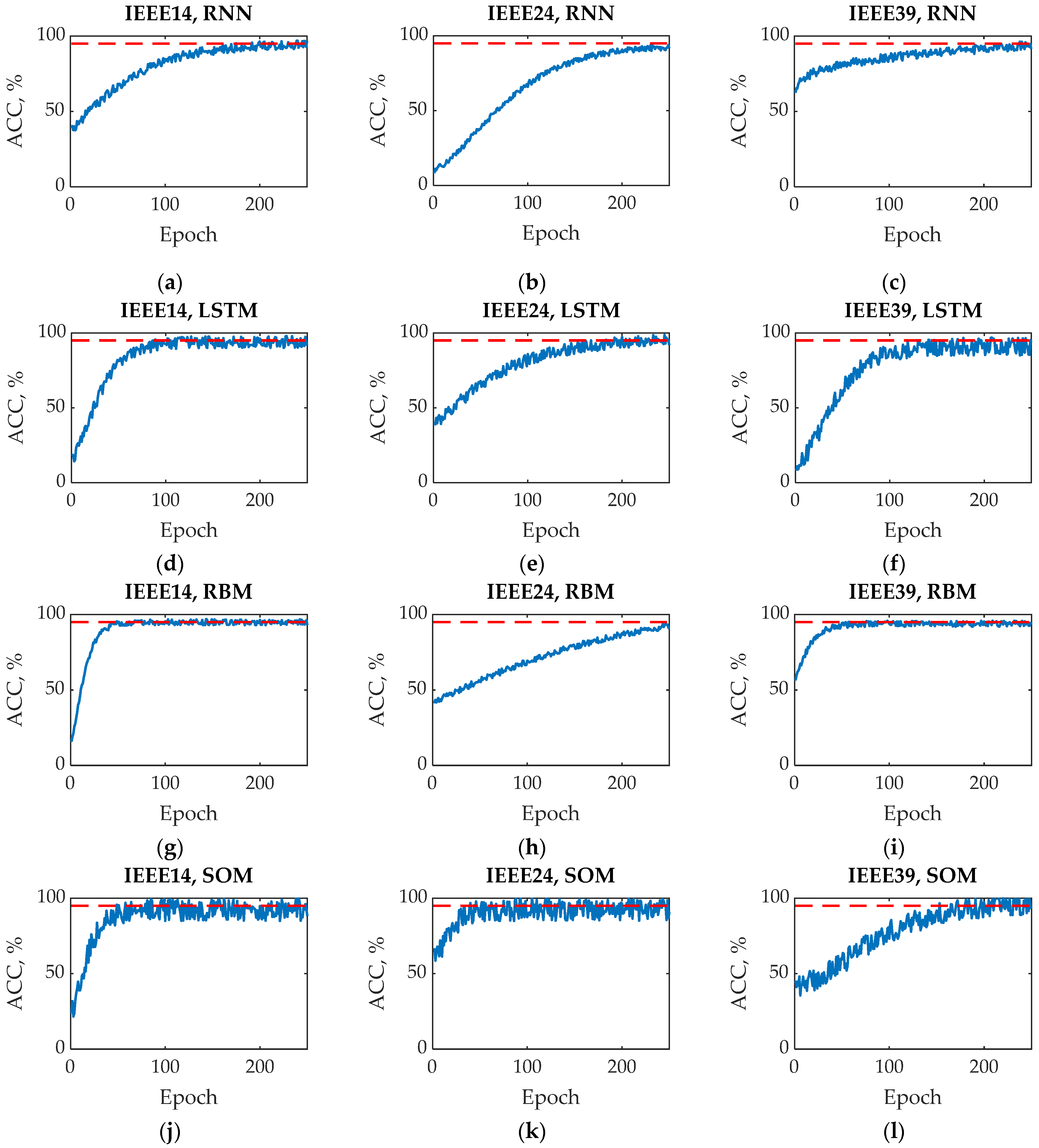
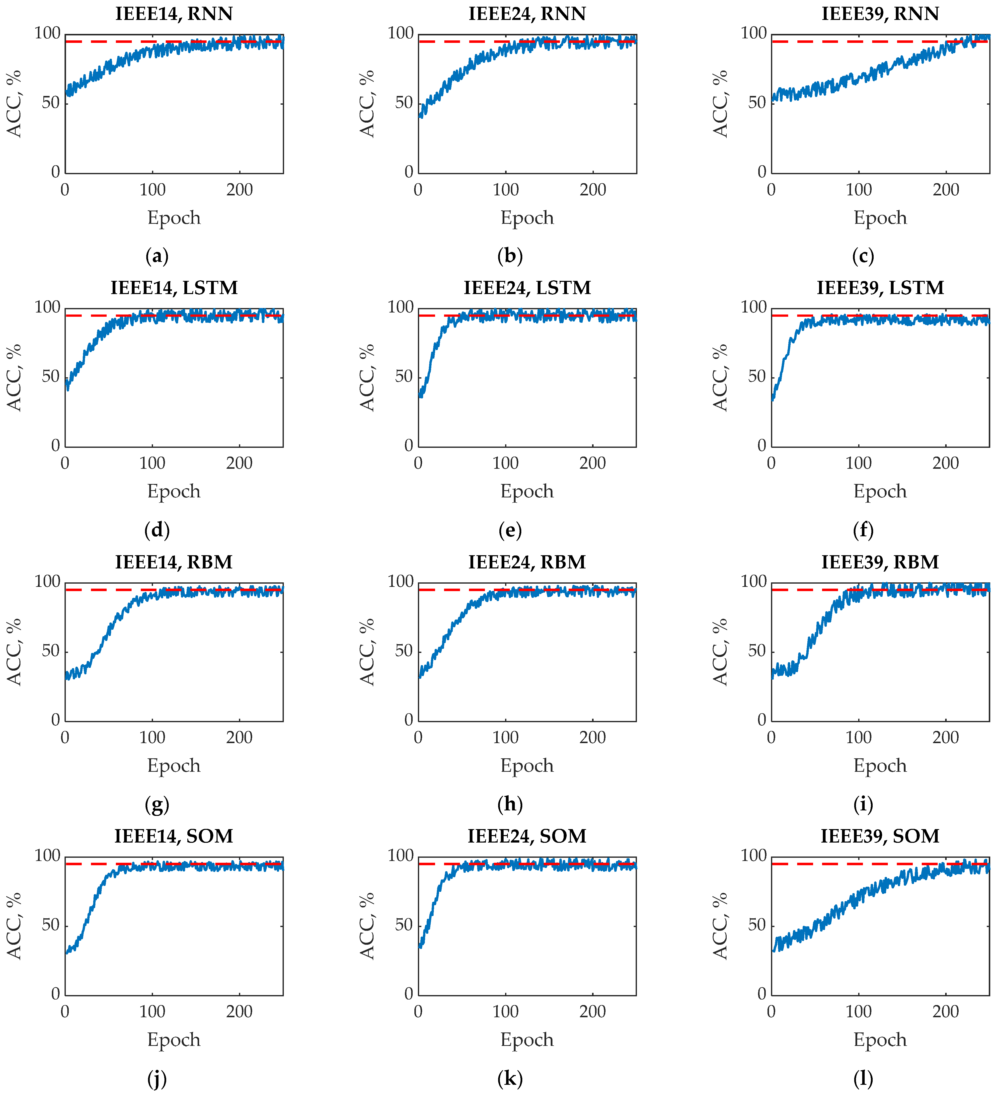
Next, the considered DL algorithms were trained and tested on a processed data sample, even without considering the voltage phase values that can be measured by PMUs. During testing, the following classification accuracy characteristics were analyzed: MDRs, FARs, ACCs, and AUCs. Table 21 shows the average values for the IEEE14, IEEE24, and IEEE39 models of the ACC ratio of the RNN, LSTM, RBM, and SOM algorithms.

Table 21. Average values of ACC ratio of the RNN, LSTM, RBM, and SOM algorithms.

Algorithm	ACC, %
Without PMU data
RNN	93.31
LSTM	94.31
RBM	93.57
SOM	92.12
With PMU data
RNN	93.18
LSTM	94.45
RBM	93.58
SOM	92.12

As a result of testing, it was found that the maximum accuracy corresponds to the LSTM algorithm. The ACC value for the LSTM algorithm is shown in bold in Table 21.

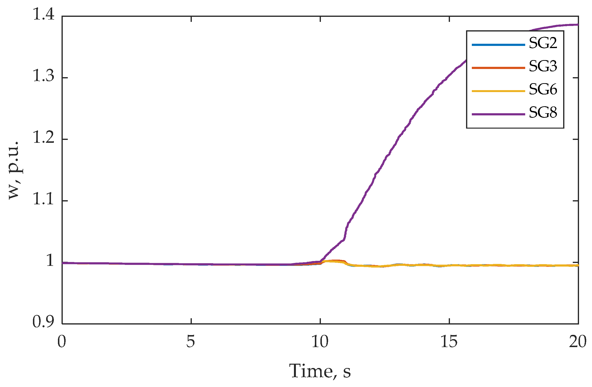
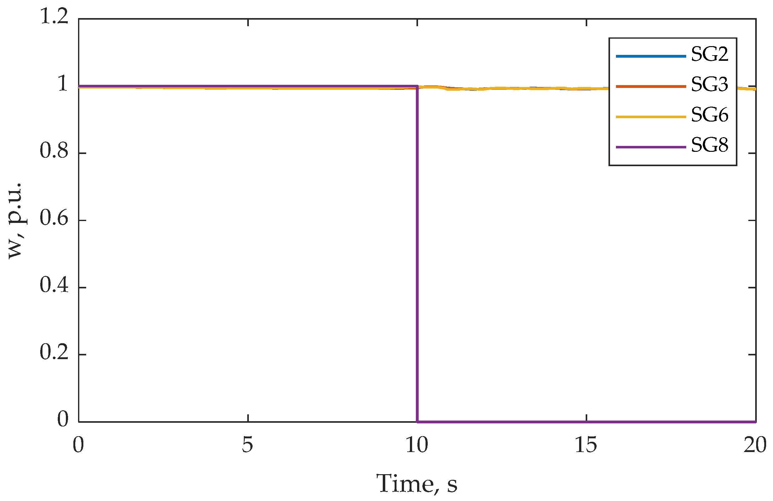
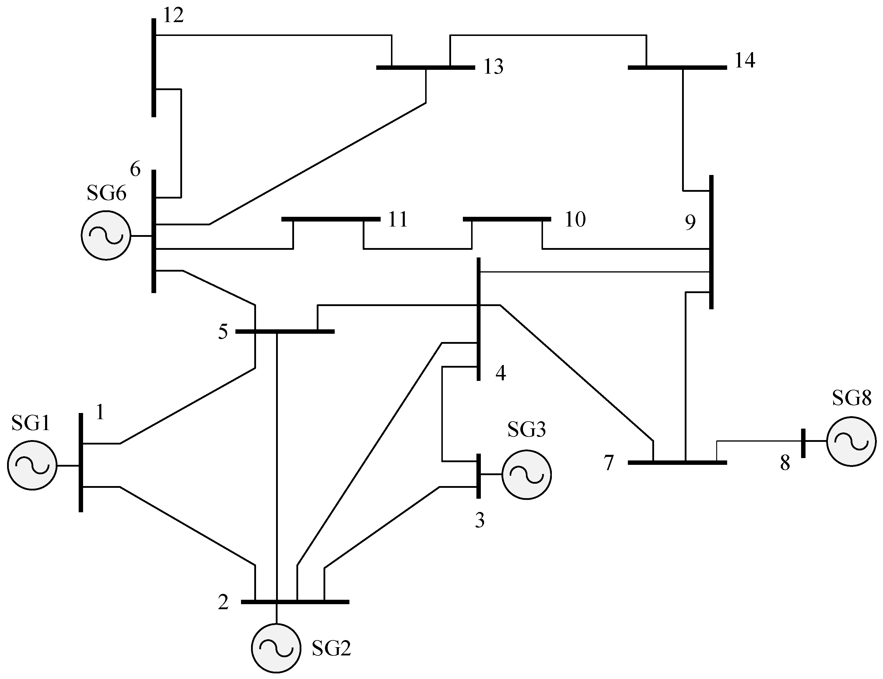
To test the possibility of selecting a CA for an accident that is missing in the data sample, for the IEEE14 model, an accident consisting of a short circuit in node 9 was considered. As a result of modeling this accident, SG8 and SG3 lose stability and operate in asynchronous mode. To provide TS, the CA was chosen in the form of SG8 shutdown. The correctness of this CA is confirmed by the results of the calculation of the transient process.

Further research will be aimed at developing a methodology for EC with isolated EPSs which contains a significant proportion of RESs and energy storage devices. For EPS data, the CAs are considered to provide the required AC voltage and frequency levels. Moreover, there are other important directions for future research. For instance, more detailed testing of the ability of DL algorithms to select optimal CAs for accidents that are not in the training set; the determination of acceptable values of time delays of DL algorithms, allowing us to define the optimal value of CAs during the development of the transient process; the determination of the minimum size of the data set; and the analysis of the influence of errors in data synchronization from PMU devices based on the accuracy of CA EPS selection are required.