Transformer-Based Composite Language Models for Text Evaluation and Classification

Abstract

Parallel natural language processing systems were previously successfully tested on the tasks of part-of-speech tagging and authorship attribution through mini-language modeling, for which they achieved significantly better results than independent methods in the cases of seven European languages. The aim of this paper is to present the advantages of using composite language models in the processing and evaluation of texts written in arbitrary highly inflective and morphology-rich natural language, particularly Serbian. A perplexity-based dataset, the main asset for the methodology assessment, was created using a series of generative pre-trained transformers trained on different representations of the Serbian language corpus and a set of sentences classified into three groups (expert translations, corrupted translations, and machine translations). The paper describes a comparative analysis of calculated perplexities in order to measure the classification capability of different models on two binary classification tasks. In the course of the experiment, we tested three standalone language models (baseline) and two composite language models (which are based on perplexities outputted by all three standalone models). The presented results single out a complex stacked classifier using a multitude of features extracted from perplexity vectors as the optimal architecture of composite language models for both tasks.

1. Introduction

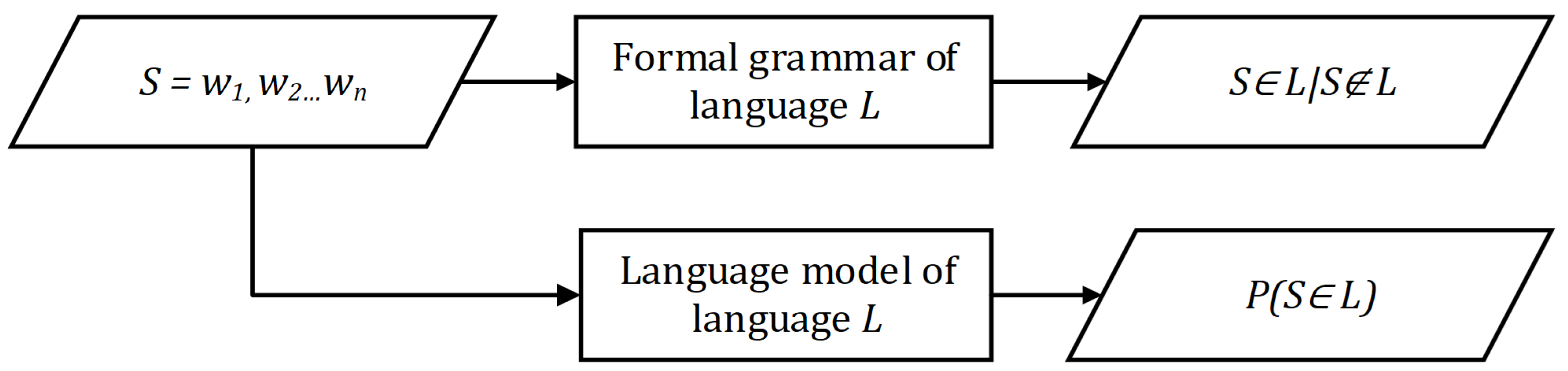
Nearing the end of the twentieth century, the accelerated development of artificial intelligence (especially machine learning methods) rekindled the idea that good results are obtainable in a much faster way and in many engineering spheres, including language modeling. In practice, it was established that one of the biggest disadvantages of formal grammar (language modeling state-of-the-art at the time) was the high cost of their creation. The extraction of grammatical rules from the corpus of texts can, of course, be carried out simply by making a list, but this leads to the problem of over-fitting the model, where individual rules are taken for general ones and the broader picture is lost. On the other hand, the derivation of general rules from individuals must be carried out carefully and requires an enormous amount of time. With new technological developments, however, the researchers began to investigate the creation of completely new probability-based models, which emulate automata and rule-based grammars. Instead of assigning a Boolean response to input strings, these new systems, called language models, assign probabilities based on a previously observed textual (training) corpus (Figure 1).

Language models are thus defined as systems that assign probabilities to strings (based on the context in which they occur), and the models are based on the previously collected corpus. Input strings refer to sequences of tokens $(w_1,w_2\dots w_n)$, usually representing n-grams of words or characters.

In the previous couple of decades, language modeling was developed primarily using artificial neural networks (ANNs), according to the inspiring idea of Elman [1,2], who, while experimenting with time series as input data for machine learning (ML) models, constructed an artificial neural network whose goal was to predict the next element in a sequence. Although the potential of using ANNs for language modeling was recognized early on, the limitations imposed by this approach caused a stagger in development. A large amount of training data necessary for the correct generalization of grammatical rules, as well as satisfactory computing resources (especially working memory and processing power), were not available (at least not to the general public) at the time of the methodology’s development. In addition, the problem of the vanishing gradient, a consequence of backpropagation when training multi-layer and recurrent ANNs, was observed often in practice [3], especially on the task of natural language modeling.

Nevertheless, the exponential growth in the PC computing power that followed, as well as the exponential increase in the amount of data available (via the Big Data phenomenon), enabled the theory to finally be technologically supported, triggering a new wave of fresh research, based on the idea of deep learning [4], which is currently the most represented sub-field of machine learning research, and artificial intelligence in general. The use of the long short-term memory method (LSTM) [5] in language modeling solved the problem of the vanishing gradient at first glance, while also providing previously unattainable results.

1.1. State-of-the-Art

Only with the emergence of the Transformer architecture by Google [6], as an adequate alternative to LSTM models, a new step forward was made in the field of natural language modeling. The main difference between transformers and LSTM models is that transformers do not rely on recurrent structures, but have an improved model for attention, a special parameter propagated during learning, which serves to separate relevant from irrelevant information. Today, the most significant and widespread language models are built using this architecture, i.e., an encoder-decoder structure for model training, supported by pre-trained word vectorizations (word embeddings) for preprocessing.

The first outstandingly influential of the type models were BERT (bidirectional encoder representations from transformers) by Google [7] and GPT (generative pre-trained transformer) by OpenAI [8,9]. The former is an encoder-based model used primarily for text annotation and classification and the latter is a decoder-based model used primarily for language generation (prediction of the next token for some given left context). Fast forward to today, decoder-based language models are most prominent in the field, with the OpenAI GPT models (now in the fourth generation) being especially popular for instruction tuning [10]. However, their last model published in open code (and also the latest one available for Serbian) is still GPT-2 [11], with the efforts still being focused mainly on the development of encoder-based models both for Serbian [12] and similar Slavic languages [13,14,15,16].

1.2. Text Quality Evaluation and Perplexity

With the beginning of the twenty-first century and the emergence of the Big Data phenomenon, the necessity to separate significant, quality data from unusable or non-quality data became even more apparent. Machine-based classification methods that rely on automatically collected attributes such as user ratings or predefined expressions (e.g., [17]) are widely used today and represent the basis for web-originated data analysis.

Classical assessment methods such as evaluation by users or experts tend to be subjective, but an adequate alternative still does not exist. Evaluating the quality of a stimulus (irrelevant of its nature) must be subjective because different people perceive it differently. The evaluation metrics vary depending on the natural language processing (NLP) task, the phase (the model building, deployment, production phase), the focus (intrinsic and extrinsic, ML and business), etc. [18]. The extrinsic metric focuses on evaluating performance on the final objective of the concrete NLP task, while the intrinsic focuses on intermediary objectives.

Intrinsic evaluation metrics have the advantage of not relying on specific tasks or reference texts, but rather on the (language) models previously trained on reference texts, which are taken as the gold standard. A typical application of intrinsic metrics is to compare two models and analyze how likely they are to generate the same text. The most common intrinsic metric used in computational linguistics is perplexity, a measure of how much the model is surprised by seeing new input text. Another way to think about perplexity is to treat it as the weighted average branching factor of a language, i.e., the average number of possible next words that can follow any word [19].

Definition 1. 

Let $\mathcal{LM}$ be a language model. Perplexity ($PP$) of a language model $\mathcal{LM}$ on a string of tokens $W=w_1{w}_2\dots w_n$ (sentence, text) is defined as the inverse probability that a model $\mathcal{LM}$ will generate W, normalized by the number of tokens n. Accordingly, perplexity is calculated as follows:

$$P{P}_{\mathcal{LM}}\left(W\right)=P_{\mathcal{LM}}{(w_1{w}_2\dots w_n)}^{-\frac{1}{n}}$$

(1)

where $P_{\mathcal{LM}}(w_1{w}_2\dots w_n)$ is the probability that a model $\mathcal{LM}$ will generate W. If $L_{\mathcal{LM}}$ represents language generated by model $\mathcal{LM}$ and P is a probability function, then

$$P_{\mathcal{LM}}(w_1{w}_2\dots w_n)=P(w_1{w}_2\dots w_n\in L_{\mathcal{LM}})$$

(2)

This implies that the higher the value of perplexity, the poorer the fit of the tested input string and the model. If we have text that is taken as a gold standard, we can use perplexity as a measure of the quality of a model, or we can measure the quality of the generated text if we take a model as the gold standard. In both cases, we want the measure of perplexity to be as low as possible. In the worst case, if the model is completely unprepared and the probability for each token is the same, then the perplexity is equal to the size of the lexicon of tokens.

The aforementioned properties allow for perplexity to be used for automatically distinguishing between the high- and low-quality data [20], with one of the motives being the selection of data used to train new language models [21]. Perplexity can also be used for text classification based on language [22], the detection of harmful content [23], and fact checking [24].

1.3. Research Questions, Aims, Means, and Novelty

Recent developments in NLP (primarily statistically based language models) have brought us numerous new methods and technologies of language modeling [25], with new and arguably better language models appearing every so often. This paper constitutes an expansion of prior scholarly investigations dedicated to processing and evaluating texts written in arbitrary highly inflective and morphology-rich natural language, particularly Serbian. Two prior investigations considering (Serbian) language processing tasks are revisited, specifically, part-of-speech tagging [26] and literature authorship attribution [27] in order to inspect advantages of using composite language models. In these papers, several feature combination techniques were tested (e.g., voting, weighted voting, bidding), but it was concluded that the trained stacked classifier is the optimal method of feature combination, with the main advantage of distinguishing between quality and noise-inducing features. Additionally, if the trained stacked classifier’s complexity is kept low, their explicitness is reasonable and the risk of overfitting them is minimal. The specific aim of this research is to further develop the methodology for the creation of composite intelligent systems to aid in solving the task of language modeling, particularly focusing on the tasks of perplexity-based text evaluation and classification [20]. The main motivation of the experiment was to support the distinction between high-quality and low-quality text, particularly that acquired from the web, in order to secure the integrity of automatically constructed corpora.

In order to achieve this goal, a group of standalone transformer-based language models (GPT-2), previously trained on a corpus of texts in Serbian [28], were used to develop several different composite language models. The expediency of the models will be illustrated in the example of solving two binary classification tasks:

C₁

Detection of low-quality sentences;

C₂

Machine translation detection.

The first classification task was chosen because of its direct alignment with the goal of the research (distinguishing between high-quality and low-quality text), while the second task was chosen as an alternative, which is more difficult benchmark, especially with the recent advances in the field of machine translation [29]. The ability of the standalone models to classify the sentences will be tested using only the sentence perplexity value outputted by the model. The obtained results will be used as a baseline for the evaluation of the composite models. The first of the two envisioned composite models, $C{M}_1$, will use sentence perplexities outputted by each of the three standalone models (M₁, M₂, and M₃, Section 2.1) as classification features. Besides the $C{M}_1$ features, the second composite model, $C{M}_2$, will use additional features extracted from standalone models M₁, M₂, and M₃.

This paper will address three research questions:

RQ1 

Are semantic and syntactic models justified tools to use for sentence classification tasks, e.g., low-quality sentence or machine translation detection?

RQ2 

Can composite language models based on outputted perplexities and the wisdom of crowds-based compositions improve on the accuracy of standalone models on classification tasks?

RQ3 

Can features extracted from perplexity vectors be used to further improve the classification accuracy of composite models?

The main contributions of this research are:

• Development of a perplexity-based dataset for testing and validation of composite and standalone language models using existing models and parallel language corpora;
• Development of a detailed model of the composite systems for parallel unification of created models (which can be applied to both future models and other languages);
• Creation of composite Serbian language models that can be used in natural language processing tasks, including document classification and text evaluation;
• Evaluation of created models on two well-known binary classification problems.

The developed composite model architectures are to enable a more precise calculation of fitness between models and texts (i.e., a more precise calculation of perplexity) which could also induce performance improvement for generative language models. Additionally, the knowledge gathered through the inspection of the results should enable researchers to further develop the methodology of composite intelligent systems creation.

Section 2 of this paper will present the creation of the main evaluation dataset and its merits, and Section 3 will describe the process of feature extraction and model compositions. Section 4 will present the evaluation process and the results obtained, which will be followed by the discussion and concluding remarks, together with plans for future research in Section 5.

2. Dataset

The dataset used to evaluate the proposed methodology approach for this experiment is envisioned as a series of matrices containing perplexity values obtained through standalone language model evaluation. In order to prepare the dataset, several standalone language models (M₁, M₂, and M₃) that output different perplexity values for the same text were needed, and also several series of textual sentences (T₁, T₂, and T₃) not previously used for the training or fine-tuning of M₁, M₂, and M₃. The final dataset is obtained by evaluation of M₁, M₂, and M₃ using T₁, T₂, and T₃ as the test sets.

The textual dataset T was envisioned as a list of three separate sets:

T₁

High-quality sentences in Serbian, obtained from the expert translation of appraised novels written in other languages;

T₂

List of low-quality sentences, i.e., a list of sentences from the dataset T₁ corrupted using several different methods in order to make them semantically or syntactically incorrect;

T₃

List of machine translations of the original literary sentences, as opposed to the expert translations from the dataset (T₁).

The final dataset D was generated by recording the perplexity values of prepared language models against the prepared sets of sentences, and it was used to evaluate the methodology on both envisioned classification tasks. The detection of low-quality sentences (C₁) is summed up as the classification between datasets T₁ and T₂, and the detection of machine translations (C₂) as the classification between datasets T₁ and T₃. The complete process of the dataset generation can be summed up in three steps:

• Preparation of pre-trained language models for Serbian that tend to output different perplexity measures for textual input (M₁, M₂, and M₃);
• Preparation of textual data T₁, T₂, and T₃ (based on text not used for the training or fine-tuning of aforementioned language models), which will be used for the creation of evaluation dataset for both classification tasks (C₁ and C₂);
• Generation of the final dataset, based on perplexity outputs obtained via evaluation of the prepared sentences from the previous step (T₁, T₂, and T₃) using prepared language models from the first step (M₁, M₂, and M₃).

2.1. Language Models

A total of three standalone language models that were previously trained [28] on a collected corpus of Serbian texts and based on a second-generation generative pre-trained transformers architecture (GPT2, 137 million parameters) were used for this research:

M₁

Control model trained using a standard corpus of contemporary Serbian texts (1 billion tokens), and standard training configuration for GPT2-based models;

M₂

Experimental semantic model, trained on a specially prepared corpus representation, i.e., a corpus processed using latent semantic analysis methods [30], namely removal of stop words and lemmatization;

M₃

Experimental syntactic model, trained on a different corpus representation that was processed using morphological dictionaries in such a way that the content words [31] were replaced with their grammatical category.

The two experimental models were supposed to model two complementary aspects of the text in natural language (semantics and syntax) and therefore produce potentially different perplexities when faced with the same piece of input text. It should be noted that when calculating perplexity using these models, input text must be preprocessed using the same transformation that was used for the generation of the training corpus data for the respective model in order to obtain correct readings. All three of these models are available in open access on the Huggingface platform and linked in the Data Availability Statement at the end of the paper. See Appendix A for the implementation details.

2.2. Textual Data

Textual data used to build the evaluation dataset for this research is based on a parallel corpus of literary texts (novels originally written in German and Italian and their expert translations into the Serbian language). The bigger share of the texts was pooled from parallel Serbian–German corpus, SrpNemKor [32], where only the novels originally written in German were used. The rest of the textual data represent the parallel translation of the third part of the Naples stories series [33,34], prepared as the part of the parallel Serbian–Italian corpus within the It-Sr-Ner project (supported by CLARIN ERIC “Bridging Gaps Call 2022”) [35]. A total of seven novel translations were used (

Table 1. A list of novels from which evaluation sentences were extracted.

Author	Translator	Title	Sentences #
Tomas Bernhard	B. Denić	Meine Preise	1009
Elfride Jelinek	T. Tropin	Die Klavierspielerin	6679
Milo Dor	T. Bekić	Wien, Juli 1999	1249
Günter Grass	A. G. Rajić	Im Krebsgang	2868
Günter de Bruyn	A. Bajazetov-Vučen	Buridans Esel	2890
Christof Ransmayr	Z. Krasni	Die letzte Welt	3107
Elena Ferrante	J. Brborić	Storia di chi fugge e di chi resta	8316

).

The first envisioned set of $26,118$ sentences (a set of expert translations, $T_1$) was created by simply extracting sentences from the translations listed in novels. The set contains $536,639$ tokens (about $20.55$ per sentence) and has a type-token ratio of $0.1124$.

The second set (low-quality sentences, $T_2$) was created by taking each sentence from the first set and applying one of the following transformations at random:

• Lemmatization: Each word in the sentence is replaced with its lemma based on Serbian Morphological Dictionaries, to make the sentences prone to morphosyntactic incorrectness. Although it is possible that the lemmatized sentence is equal to the original one (in case all words in the original sentence were already lemmas), a simple equality comparison between them calculated that this happens less than 0.8% of the time;
• Random mixing of word order within a sentence: A sentence was transformed into a list of words and punctuation marks, which was then randomly shuffled and put back together into text. This was also conducted to make the sentences prone to syntactical incorrectness, especially regarding the position of prepositions and adjectives. As in the previous case, this does not necessarily mean that the sentences are incorrect, but a manual evaluation of a set of 400 sentences found that this happens in less than 0.6% of the cases;
• Random replacement of words in the sentence: namely, each word in the sentence is replaced by another, random word of the same grammatical category from the Serbian Morphological dictionaries, in order to make it prone to semantic incorrectness.

The application of these transformations does not affect sentence lengths, but the type-token ratio is decreased to $0.0902$ (due to the lemmatization of one part of the sentences).

The third set of sentences (machine translations, $T_3$) was obtained by running the original sentences (in German and Italian) through the Google Translate service and translating them into Serbian. Another simple equality comparison revealed that they differ from expert translations about $98\%$ of the time. These sentences are somewhat shorter (average of $19.03$ tokens per sentence and $496,989$ total), but the type-token ratio of $0.1106$ is quite similar to the one of the first set.

The complete textual dataset $T={\bigcup }_{j=1}^3{T}_j$ is a sequence comprising $78,354$ sentences divided into three subsequences $T_j$ of equal size $|T_j|=26,118$.

2.3. Sentence Perplexities and Perplexity Vectors

Definition 2. 

Let $i,j\in \mathbb{Z}$. Integer interval $[i ..j]$ is defined as $\{k\in \mathbb{Z}\mid i\le k\le j\}$.

Definition 3. 

Let $x={\left(x_i\right)}_{i=1}^n\in {\mathbb{R}}^n$ and ${\prod }_{i=1}^n{x}_i\ne 0$. The vector $x^{\circ -1}={\left(\frac{1}{x_i}\right)}_{i=1}^n$ is the element-wise inverse (also called Hadamard inverse) of vector x.

Definition 4. 

Perplexity vector ($PPV$) [36] of a language model $\mathcal{LM}$ on a sentence $s=w_1{w}_2\dots w_n$ is calculated applying the Equation (1) to each N-gram of tokens within a sentence (N fixed, $N\in [1 ..n]$):

$$PP{V}_{\mathcal{LM}}\left(s\right)=PP{V}_{\mathcal{LM}}(w_1{w}_2\dots w_n)=\left[\begin{array}{c}{P}_{\mathcal{LM}}{(w_1{w}_2\dots w_N)}^{-\frac{1}{N}}\\ P_{\mathcal{LM}}{(w_2{w}_3\dots w_{N+1})}^{-\frac{1}{N}}\\ ⋮\\ P_{\mathcal{LM}}{(w_{n-N+1}{w}_{n-N+2}\dots w_n)}^{-\frac{1}{N}}\end{array}\right]$$

(3)

Size $N=5$ is used during this experiment. The size of $PPV$ for a given sentence s is $n-N+1$ and therefore varies depending on the number of tokens n in s.

Let $i,j,k\in \mathbb{N}$, $i,j\in [1 ..3]$, $k\in [1 ..m]$. The final dataset D consists of:

D₁

Subset containing three sequences of inverse perplexity triples, one for each dataset $T_j$, i.e.,

$${(\frac{1}{p{p}^{\left(jk\right)}\left[1\right]},\frac{1}{p{p}^{\left(jk\right)}\left[2\right]},\frac{1}{p{p}^{\left(jk\right)}\left[3\right]})}_k$$

(4)

where $p{p}^{\left(jk\right)}\left[i\right]$ represents perplexity of the model $M_i$ on the kth sentence in the dataset $T_j$, calculated using (1). See Appendix A for the implementation details.

D₂

The subset comprised three sequences, one for each dataset $T_j$, where every sequence element is a triple containing the Hadamard inverse of perplexity vectors, i.e.,

$${({\left(pp{v}^{\left(jk\right)}\left[1\right]\right)}^{\circ -1},{\left(pp{v}^{\left(jk\right)}\left[2\right]\right)}^{\circ -1},{\left(pp{v}^{\left(jk\right)}\left[3\right]\right)}^{\circ -1})}_k$$

(5)

and $pp{v}^{\left(jk\right)}\left[i\right]$ represents the perplexity vector of the model $M_i$ on the kth sentence in the dataset $T_j$, calculated using (3).

Values stored in sets $D1$ and $D2$ were used to measure the classification performance of (both standalone and composite) language models on the tasks of detecting low-quality sentences and machine translations (see Section 4).

Definition 5. 

Let ${\left(x_i\right)}_{i=1}^n$ and ${\left(y_i\right)}_{i=1}^n$ be two sequences of length n. The Pearson linear correlation coefficient r is defined as

$$r=\frac{{\sum }_{i=1}^n\left(x_i-\overline{x}\right)\left(y_i-\overline{y}\right)}{\sqrt{{\sum }_{i=1}^n{(x_i-\overline{x})}^2{\sum }_{i=1}^n{(y_i-\overline{y})}^2}},$$

(6)

where $\overline{x}=\frac{1}{n}{\sum }_{i=1}^n{x}_i$ represents the mean of x and analogously for $\overline{y}$.

Let $i,j,k,l\in [1 ..3]$ and $M_i{T}_j$ be a sequence ${\left(p{p}^{\left(jk\right)}\left[i\right]\right)}_k$ such that $|M_i{T}_j|=|T_j|=m$, i.e., a sequence of perplexity values obtained for sentences of dataset $T_j$ using model $M_i$. In order to ensure that the perplexity values differ between both different models and different textual datasets, the Pearson coefficients $r_{ijkl}$ were calculated using (6), as the primary measure of linear correlation between every two pairs $M_i{T}_j$ and $M_k{T}_l$, where pairs share either a model ($i=k$) or a dataset ($j=l$).

Table 2. Pearson correlation coefficients between sequences of perplexities obtained using two different pairs (model, dataset) $M_i{T}_j$ with the mutual dataset.

Model	${\mathit{M}}_1{\mathit{T}}_1$	${\mathit{M}}_2{\mathit{T}}_1$	${\mathit{M}}_3{\mathit{T}}_1$
$M_1{T}_1$		0.265	0.044
$M_2{T}_1$	0.265		−0.019
$M_3{T}_1$	0.044	−0.019
	$M_1{T}_2$	$M_2{T}_2$	$M_3{T}_2$
$M_1{T}_2$		0.166	0.174
$M_2{T}_2$	0.166		−0.116
$M_3{T}_2$	0.174	−0.116
	$M_1{T}_3$	$M_2{T}_3$	$M_3{T}_3$
$M_1{T}_3$		0.225	0.065
$M_2{T}_3$	0.225		−0.060
$M_3{T}_3$	0.065	−0.060

and

Table 3. Pearson correlation coefficients between sequences of perplexities obtained using different pairs (model, dataset) $M_i{T}_j$ with the mutual model.

	${\mathit{M}}_1{\mathit{T}}_1$	${\mathit{M}}_1{\mathit{T}}_2$	${\mathit{M}}_1{\mathit{T}}_3$
$M_1{T}_1$		0.515	0.645
$M_1{T}_2$	0.515		0.369
$M_1{T}_3$	0.645	0.369
	$M_2{T}_1$	$M_2{T}_2$	$M_2{T}_3$
$M_2{T}_1$		0.803	0.512
$M_2{T}_2$	0.803		0.419
$M_2{T}_3$	0.512	0.419
	$M_3{T}_1$	$M_3{T}_2$	$M_3{T}_3$
$M_3{T}_1$		0.790	0.676
$M_3{T}_2$	0.790		0.544
$M_3{T}_3$	0.676	0.544

contain the resulting $r_{ij}$ coefficients between $M_i{T}_j$ pairs, where pairs share the same dataset in Table 2, while pairs in Table 3 share the same model.

The results presented in Table 2 confirm the uniqueness of perplexities outputted using the prepared models, with the highest correlation coefficient being 0.265 between the models M₁ (control) and M₂ (semantic) and all of the other correlation coefficients being less than 0.05. On the other hand, the much higher correlation was apparent in Table 3, averaging at about 0.56, indicating that the models have trouble differing between the datasets, especially model M₂ between the datasets T₁ and T₂ (inability to distinguish the control set from the artificially-defected, low-quality sentences), with a correlation coefficient of over 0.8. In Section 3, we introduce composite models as a form of overcoming this insufficiency.

Once the data were confirmed to be of value, all of the perplexity values in sets D₁ and D₂ were converted to their inverse value, which concluded the creation of the dataset D according to Equations (4) and (5). This was carried out for the sake of their easier input into the machine learning algorithms afterwards in the experiment.

3. Features and Compositions

As mentioned in Section 1.3, two composite models, $C{M}_1$ and $C{M}_2$, built on the resulting perplexities were envisioned for this experiment. The first, simpler model (Section 3.1) is based on a stacked classifier architecture which is directly derived from the previous research on the subject [26,27]. The second, more complex model (Section 3.2) was designed specially for this experiment and relies on features extracted using several different scenarios.

3.1. Simple Neural Network Classifier ($C{M}_1$)

The stacked sentence classifier used in the first composition ($C{M}_1$) is based on a simple neural network architecture consisting of one fully connected layer—two perceptrons, one for each class, sharing a triple of input values $p=(P_1,P_2,P_3)$, an element of dataset D₁. The triple p corresponds to a sentence being classified and each $P_i$ is an inverse of the perplexity value of model $M_i$, $i,j\in [1 ..3]$ (Figure 2).

The $C{M}_1$ output y is the predicted class of the sentence. The value of y can be either 0, meaning expert translation, or 1, meaning an alternative class the network was trained to recognize, depending on the classification task. The calculation of y can be described in the following manner:

$$y=f(p{W}^T+b)=p{W}^T+b$$

(7)

where:

• $p=(P_1,P_2,P_3)\in {\mathbb{R}}^3$ is a triple containing inverse of perplexities corresponding to the input sentence;
• $W=\left(w_{ij}\right)\in {\mathbb{R}}^{2\times 3}$ is a weight matrix. For a fixed $i\in [1 ..2]$, ${\left(w_{ij}\right)}_j\in {\mathbb{R}}^3$ are learnable weights of the ith perceptron in $C{M}_1$, $j\in [1 ..3]$;
• $b\in {\mathbb{R}}^2$ components are learnable biases of the corresponding perceptrons in $C{M}_1$;
• f is an activation function defined as identity $f\left(z\right)=z$, i.e., linear activation is used.

See Appendix A for the implementation details and Section 4 for training details.

The goal of this model was to confirm the advantages of using a stacked classifier on the perplexity outputs of transformer-based language models, as was already confirmed for using it on probabilistic outputs of part-of-speech taggers [26] and cosine similarities of documents before that [27], in order to give an answer to RQ2.

3.2. Complex Multi-Featured Neural Network ($C{M}_2$)

In contrast to $C{M}_1$ (Section 3.1), the second composite model ($C{M}_2$) was designed to maximize the volume of inputted features at the expense of simplicity. The goal of the feature extraction for this experiment was to create a large, determined, and finite list of inputs for a binary classifier; hence, all of the features are represented as numerical values in the range −1 to 1. In addition to the three features used by $C{M}_1$, a multitude of additional features are extracted from subset D₂ (Section 2.3), using three separate neural network components:

NN₁

The time-and-frequency-domain-based component represents a small, single-layer neural network used to extract eight features from a multitude of properties calculated using a set of prepared formulas over each vector from D₂ (see Section 3.2.1);

NN₂

The recurrent neural network (RNN) [37] component represents a small neural network with a recurrent layer with four hidden states. Vector triples from dataset D₂ are inputted into this layer in order to extract four additional features for each triple (see Section 3.2.2);

NN₃

The convolutional neural network (CNN) [38] component represents a small neural network with a convolutional and a pooling layer instead of a recurrent one, which is used to extract eight more features from each vector triple of dataset D₂ (see Section 3.2.3).

For the purpose of training components $N{N}_2$ and $N{N}_3$, the length of the vector inputs (extracted from the $D_2$ set) for these two components was resized to the length ${\displaystyle \mathit{\ell }}=64$, employing either truncation (if the vector was longer) or zero-padding (if the vector was shorter). This was conducted for the purpose of easier batching of vector inputs during the training procedure for recurrent and convolutional layers. The $N{N}_1$ component uses the original vectors. All of the mentioned components are connected to one final component:

NN₄

The classifying component represents a neural network with two fully connected layers that takes all of the aforementioned features as input and then outputs the class of the inspected sentence.

The four components are trained together as one binary classification system (for each of two envisioned classification tasks) in order to give a definite answer to RQ3.

3.2.1. Time-and-Frequency-Domain-Based Component ($N{N}_1$)

The first $C{M}_2$ component is used to extract features from different time-domain and frequency-domain properties of the vectors from dataset D₂, while treating them as either time-series (by using tokens as a unit of time and inspecting the perplexity value at each point) or signals. In the case of time-domain ($TD$), the twelve properties TD₁–TD₁₂ were examined using each vector as an input for twelve different formulas. Some of them are reused to examine six frequency-domain ($FD$) properties FD₁–FD₆, but the input is changed to be a power spectrum calculated using a fast Fourier transform of each vector.

The following time-domain properties were determined for vector $x={\left(x_i\right)}_{i=1}^n$:

TD₁

Minimum value found in the inspected vector:

$$Min\left(x\right)=\underset{i\in [1..n]}{min}{x}_i;$$

(8)

TD₂

Maximum value found in the inspected vector:

$$Max\left(x\right)=\underset{i\in [1..n]}{max}{x}_i;$$

(9)

TD₃

Peak-to-peak, calculated as the difference between the maximum and minimum value:

$$P_k\left(x\right)=Max\left(x\right)-Min\left(x\right);$$

(10)

TD₄

The arithmetic mean of the values in the inspected vector:

$$\overline{x}=\frac{1}{n}\sum _{i=1}^n{x}_i;$$

(11)

TD₅

Root mean square:

$$RMS\left(x\right)=\sqrt{\frac{1}{n}\sum _{i=1}^n{x_i}^2};$$

(12)

TD₆

Variance, i.e., the spread of data around the mean:

$${\sigma }^2=\frac{1}{n}\sum _{i=1}^n{(x_i-\overline{x})}^2;$$

(13)

TD₇

The standard deviation of the inspected vector:

$$\sigma =\sqrt{\frac{{\sum }_{i=1}^n{(x_i-\overline{x})}^2}{n-1}};$$

(14)

TD₈

Crest factor, i.e the quotient of the maximum value and the root mean square:

$$CF\left(x\right)=\frac{Max\left(x\right)}{RMS\left(x\right)};$$

(15)

TD₉

Form factor, i.e., the quotient of the root mean square and mean:

$$FF\left(x\right)=\frac{RMS\left(x\right)}{\overline{x}};$$

(16)

TD₁₀

Pulse indicator, i.e., the quotient of the maximum value and the mean of the vector:

$$PI\left(x\right)=\frac{Max\left(x\right)}{\overline{x}};$$

(17)

TD₁₁

Vector (Pearson) kurtosis, i.e., the measure of the outlier presence in the inspected vector:

$${\beta }_2=\mathbb{E}\left[{\left(\frac{x-\overline{x}}{\sigma }\right)}^4\right],$$

(18)

where $\mathbb{E}$ is the expectation operator;

TD₁₂

Vector skewness, i.e., the measure of the data symmetry around the mean:

$${\gamma }_1=\mathbb{E}\left[{\left(\frac{x-\overline{x}}{\sigma }\right)}^3\right],$$

(19)

where $\mathbb{E}$ is the expectation operator.

As the second set of properties is based in the frequency domain, each vector was first subjected to the fast discrete Fourier transform, calculating a new vector ${\left({\mathcal{F}}_k\right)}_{k\in [0..n-1]}\in {\mathbb{C}}^n$:

$${\mathcal{F}}_k=\sum _{j=1}^n{x}_j{e}^{-\frac{2i\pi }{n}k(j-1)},k\in [0 ..n-1],$$

(20)

where n is the length of the vector x that is being transformed and $i\in \mathbb{C}$ is the imaginary unit, $i^2=-1$.

Afterwards, the power spectrum vector $y={\left(y_k\right)}_{k\in [0..n-1]}$ is calculated:

$$y_k=\frac{|{{\mathcal{F}}_k}^2|}{n},k\in [0 ..n-1].$$

(21)

With the calculated power spectrum of the vector, the following frequency-domain properties were extracted:

FD₁

Power spectrum maximum, calculated using Equation (9), where x is the power spectrum of the inspected vector;

FD₂

Power spectrum peak, calculated as the absolute maximum value found in the power spectrum:

$$P_m=\underset{i\in [1..n]}{max}\left|x_i\right|,$$

(22)

where x is the power spectrum of the inspected vector;

FD₃

Power spectrum mean, calculated as an arithmetic mean of the values in the power spectrum using Equation (11), where n is the length of the power spectrum x;

FD₄

Power spectrum variance, calculated using Equation (13), where n is the length of the power spectrum x and $\overline{x}$ is its sample mean;

FD₅

Power spectrum kurtosis, calculated using Equation (18), where $\overline{x}$ is the mean of the power spectrum vector x, $\sigma$ its standard deviation, and $\mathbb{E}$ is the expectation operator;

FD₆

Power spectrum skewness, calculated using Equation (19), where $\overline{x}$ is the mean of the inspected vector x, $\sigma$ its standard deviation, and $\mathbb{E}$ is the expectation operator.

These 54 properties (18 for each vector in a D₂ dataset triple) are used as an input for a simple fully connected layer in order to extract eight final features ${\left(F_j\right)}_{j=1}^8$ as depicted in Figure 3. This was conducted in order to reduce the total number of features, as well as to extract only their most important aspects. The rectified linear unit function (ReLU) is applied to the output in order to prepare it for passing through the adjacent linear layer in $N{N}_4$. The neural network component is visualized in Figure 3. The calculation of the features can thus be described as follows:

$${\left(F_j\right)}_{j=1}^8=ReLU(g{W}^T+b)$$

(23)

where:

• $g\in {\mathbb{R}}^{54}$ is a series of time-domain and frequency domain properties extracted from the triple containing the Hadamard inverse of perplexity vectors using TD₁–TD₁₂ and FD₁–FD₆, corresponding to the input sentence;
• $W=\left(w_{ij}\right)\in {\mathbb{R}}^{8\times 54}$ is a weight matrix; ${\left(w_{ij}\right)}_j\in {\mathbb{R}}^{54}$ are learnable weights of the ith perceptron of $N{N}_1$, $i\in [1 ..8]$, $j\in [1 ..54]$;
• Components of $b\in {\mathbb{R}}^8$ are learnable biases of the corresponding perceptrons of $N{N}_1$;
• If $z={\left(z_i\right)}_{i=1}^8\in {\mathbb{R}}^8$, $ReLU$ is a rectified linear unit function defined as $ReLU\left(z\right)={\left(ReLU\left(z_i\right)\right)}_{i=1}^8={(max(0,z_i))}_{i=1}^8$.

See Appendix A for the implementation details.

3.2.2. RNN Component ($N{N}_2$)

A second set of features ${\left(F_j\right)}_{j=9}^{12}$ was extracted using a recurrent neural network component (Figure 4). One recurrent layer with four hidden states $h={\left(h^{\left(j\right)}\right)}_{j=1}^4$ was used to process each D₂ dataset triple of vectors $x=(x^{\left(1\right)},x^{\left(2\right)},x^{\left(3\right)})$, where $x^{\left(i\right)}\in {\mathbb{R}}^{{\displaystyle \mathit{\ell }}}$, $i\in [1 ..3]$, and ℓ is the resized length of input vector, introduced at the beginning of Section 3.2. For each $t\in [1 ..{\displaystyle \mathit{\ell }}]$, a triple $x_t=(x_t^{\left(1\right)},x_t^{\left(2\right)},x_t^{\left(3\right)})\in {\mathbb{R}}^3$ is processed with hidden states $h_{t-1}=(h_{t-1}^{\left(1\right)},h_{t-1}^{\left(2\right)},h_{t-1}^{\left(3\right)},h_{t-1}^{\left(4\right)})\in {\mathbb{R}}^4$ from the previous loop pass-through (if any) with the goal to extract a number of recurrent features.

The calculation of the hidden state values is performed as follows:

$$h_t=tanh(x_t{W}_{ih}^T+b_{ih}+h_{t-1}{W}_{hh}^T+b_{hh}),t\in [1 ..{\displaystyle \mathit{\ell }}],$$

(24)

where:

• $h_t\in {\mathbb{R}}^4$ is the hidden state at time t. The initial hidden state at time 0 is $h_0$ = 0 $\in {\mathbb{R}}^4$;
• $x_t\in {\mathbb{R}}^3$ is the input at time t;
• $W_{ih}\in {\mathbb{R}}^{4\times 3}$ are the learnable input-hidden weights of the (only) layer (4 hidden states, 3 input values) of $N{N}_2$;
• $b_{ih}\in {\mathbb{R}}^4$ is the learnable input-hidden bias of the (only) layer of $N{N}_2$;
• $W_{hh}\in {\mathbb{R}}^{4\times 4}$ are the learnable hidden-hidden weights of the (only) layer of $N{N}_2$;
• $b_{hh}\in {\mathbb{R}}^4$ is the learnable hidden-hidden bias of the (only) layer of $N{N}_2$;
• tanh is the hyperbolic tangent activation function.

See Appendix A for the implementation details.

The recurrent layer outputs (from four hidden states after the final pass-through) are taken as four extracted features ${\left(F_j\right)}_{j=9}^{12}=h_{{\displaystyle \mathit{\ell }}}$. The visualization of the component is depicted in Figure 4.

3.2.3. CNN Component ($N{N}_3$)

Definition 6. 

For finite discrete functions $f,g\in {\mathbb{C}}^N$, $N\in \mathbb{N}$, the (circular) cross-correlation [39] is defined as:

$$(f★g)\left[n\right]=\sum _{m=0}^{N-1}\overline{f\left[m\right]}g\left[{(m+n)}_{\mathit{mod}N}\right]$$

(25)

A somewhat more complicated process was the extraction of the final eight features from the triples using the convolutional architecture, comprising three layers:

• A one-dimensional convolutional layer with three input channels ($C_{in}=3$), eight output channels ($C_{out}=8$), a size-five kernel ($K_c=5$), and a stride of two ($S_c=2$);
• A one-dimensional max pooling layer [40] with a size-five kernel ($K_p=5$) and stride of two ($S_p=2$);
• A fully connected linear layer with an input layer with a size corresponding to the number of features extracted using the previous (pooling) layer and the output size of eight. Just like for $N{N}_1$, a ReLU activation function was applied in order to prepare features for passing through the first layer of the $N{N}_4$ component.

During the processing of input $x=(x^{\left(1\right)},x^{\left(2\right)},x^{\left(3\right)})$ using the first layer, the kernel is sliding simultaneously across the values in all three vectors $x^{\left(j\right)}\in {\mathbb{R}}^{{\displaystyle \mathit{\ell }}}$, $j\in [1 ..3]$, extracting eight features for each inspection. The total number of inspections performed, m, is calculated as follows:

$$m=⌊\frac{{\displaystyle \mathit{\ell }}-K_c}{S_c}⌋+1$$

(26)

where ℓ is the resized and fixed length of the inputted sequences (${\displaystyle \mathit{\ell }}=64$), $K_c$ the size of the kernel ($K_c=5$), and $S_c$ stride length ($S_c=2$). Features outputted for each inspection $co=\left(c{o}_{ij}\right)\in {\mathbb{R}}^{m\times C_{out}}$ are calculated in the following manner:

$$c{o}_{ij}=b_j+\sum _{k=1}^{C_{in}}{W}_{jk}★{\mathrm{input}}_{ik},$$

(27)

where:

• $i\in [1 ..m]$ is the inspection index;
• $j\in [1 ..C_{out}]=[1 ..8]$ is the outputted feature index;
• $k\in [1 ..C_{in}]=[1 ..3]$ is the input channel index;
• Components of $b\in {\mathbb{R}}^8$ are learnable biases of the corresponding output channels for the convolutional layer;
• $W=\left(w_{jk}\right)\in {\mathbb{R}}^{8\times 3}$ is a weight matrix; ${\left(w_{jk}\right)}_k\in {\mathbb{R}}^3$ are learnable weights of the jth output channel and kth input channel, $j\in [1 ..8]$, $k\in [1 ..3]$;
• $\mathrm{Input}=\left({\mathrm{input}}_{ik}\right)\in {\mathbb{R}}^5$ represents the inspected values for the ith inspection and for kth input channel, with inspection being defined via the kernel size ($K_c=5$) and stride ($S_c=2$).

Outputted values $co$ are then processed using a max pooling layer, where a second kernel of the same size is sliding across the values in each channel, performing the inspections and extracting the maximum value for each one. This step results in M number of new features, where M is calculated as:

$$M=\left(⌊\frac{m-K_p}{S_p}⌋+1\right)\ast C_{out},$$

(28)

where m is the number of inspection of the convolutional layer (26), $K_p$ the size of the kernel ($K_p=5$), $S_p$ stride length ($S_p=2$), and $C_{out}$ the number of convolutional layer output channels.

Values compiled using the max pooling layer $po={\left(p{o}_i\right)}_{i=1}^M$ are calculated as follows:

$$p{o}_i=\underset{j\in [1..K_p]}{max}{{\mathrm{input}}_i}_j,$$

(29)

where:

• $i\in [1 ..M]$ is the inspection index;
• $j\in [1 ..K_p]$ is the index of values within inspections;
• $K_p$ is the size of the kernel of the max pooling layer;
• $\mathrm{Input}=\left({\mathrm{input}}_i\right)\in {\mathbb{R}}^M$ represents the inspected values of the ith inspection, with inspection being defined via the kernel size ($K_p=5$), stride ($S_p=2$) and output channel of the convolutional being inspected.

Lastly, values compiled using the max pooling layer $po={\left(p{o}_i\right)}_{i=1}^M$ are used as an input for a fully connected linear layer with input size M and output size of eight, which is used to produce a final tally of eight features extracted by this specific method ${\left(F_j\right)}_{j=13}^{20}$, where the feature values are calculated in the following manner:

$${\left(F_j\right)}_{j=13}^{20}=ReLU(po·W^T+b)$$

(30)

where:

• $po$ is an array of features outputted from the max pooling layer, $po={\left(p{o}_j\right)}_{j=1}^M\in {\mathbb{R}}^M$;
• $W=\left(w_{ij}\right)\in {\mathbb{R}}^{8\times M}$ is a weight matrix; ${\left(w_{ij}\right)}_j\in {\mathbb{R}}^M$ are learnable weights of the ith perceptron in the sole linear layer in $N{N}_3$, $i\in [1 ..8]$, $j\in [1 ..M]$;
• Components of $b\in {\mathbb{R}}^8$ are learnable biases of the corresponding perceptrons of the sole linear layer in $N{N}_3$;
• If $z={\left(z_i\right)}_{i=1}^8\in {\mathbb{R}}^8$, $ReLU$ is a rectified linear unit function defined as $ReLU\left(z\right)={\left(ReLU\left(z_i\right)\right)}_{i=1}^8={(max(0,z_i))}_{i=1}^8$.

See Appendix A for the implementation details.

A complete neural network component used to extract them is visualized in Figure 5.

3.2.4. Classifying Component ($N{N}_4$)

Eight features were extracted using the first component ($N{N}_1$, Section 3.2.1), four features were extracted using the second component ($N{N}_2$, Section 3.2.2), and eight features were extracted using the third component ($N{N}_3$, Section 3.2.3) together with three values that were used by the first composition ($C{M}_1$, Section 3.1), which were used as an input for one final fully connected neural network component for binary classification. This final component consists of one input layer with input size 23 (20 for extracted features $F={\left(F_j\right)}_{j=1}^{20}$ and 3 for a triple of inverse perplexity values $p=(P_1,P_2,P_3)$), connected to the output layer via one hidden layer with eight neurons (Figure 6).

As is the same for $C{M}_1$, the output y of $C{M}_2$ is the predicted class of the sentence. The value of y can be either 0 (expert translation) or 1 (alternative class the network was trained to recognize, depending on the classification task). Calculation of the y for $C{M}_2$ can be described in the following manner:

$$y=ReLU(\left(p^{⌢}F\right){W^{\left(1\right)}}^T+b_1){W^{\left(2\right)}}^T+b_2$$

(31)

where:

• p${}^{⌢}F$$\in {\mathbb{R}}^{23}$ is a concatenation of $p=(P_1,P_2,P_3)\in {\mathbb{R}}^3$, a triple containing inverse of perplexities corresponding to the input sentence, and $F={\left(F_j\right)}_{j=1}^{20}\in {\mathbb{R}}^{20}$, a triple containing the inverse of perplexities corresponding to the input sentence;
• $W^{\left(1\right)}=\left(w_{ij}^{\left(1\right)}\right)\in {\mathbb{R}}^{8\times 23}$ is a weight matrix; ${\left(w_{ij}^{\left(1\right)}\right)}_j\in {\mathbb{R}}^{2}3$ are learnable weights of the ith perceptron in the input layer, $i\in [1 ..8]$, $j\in [1 ..23]$;
• $W^{\left(2\right)}=\left(w_{ij}^{\left(2\right)}\right)\in {\mathbb{R}}^{2\times 8}$ is a weight matrix; ${\left(w_{ij}^{\left(2\right)}\right)}_j\in {\mathbb{R}}^8$ are learnable weights of the ith perceptron in the hidden layer, $i\in [1 ..2]$, $j\in [1 ..8]$;
• Components of $b_1\in {\mathbb{R}}^8$ and $b_2\in {\mathbb{R}}^2$ are learnable biases of the corresponding perceptrons in the first ($b_1$) and second ($b_2$) fully connected layer;
• If $z={\left(z_i\right)}_{i=1}^8\in {\mathbb{R}}^8$, $ReLU$ is a rectified linear unit function defined as $ReLU\left(z\right)={\left(ReLU\left(z_i\right)\right)}_{i=1}^8={(max(0,z_i))}_{i=1}^8$.

A complete stacked classifier that uses transformer outputs as inputs is composed of all of the described components and is depicted in Figure 7. See Appendix A for the implementation details and Section 4 for training details.

4. Results

For the evaluation, we used five-fold cross-validation over dataset D, for which both subsets were split into five (nearly) equal, class-balanced chunks. For each of the five folds, a different chunk was used for testing, while the other four were used to train ten classifiers, including five for each classification task ($C_1$, $C_2$). 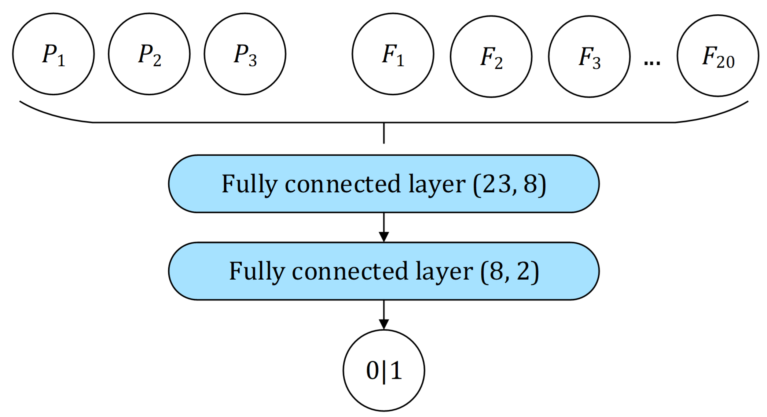Three simple classifiers were based directly on standalone models ($M_1$, $M_2$, and $M_3$), while two composite classifiers ($C{M}_1$ and $C{M}_2$) were trained on top of all three standalone models. Different training procedures were deployed depending on the classifier being trained, where different levels of input data complexity influenced the complexity of the models (

Table 4. Five classifiers used for each classification task, input data they are using (middle) (cf. Section 2), and the description of their architecture (right).

Model	Input Data	Stacked Classifier Type
$M_1$	Values from D1 dataset originated from model M1	An extension of the model in the form of a single input perceptron for binary classification, which uses that model’s (inversed) perplexity output as input
$M_2$	Values from D1dataset originated from model M2
$M_3$	Values from D1 dataset originated from model M3
$C{M}_1$	Value triples from D1 dataset, i.e., values originated from all three standalone models (M1, M2 and M3)	A simple neural network with two perceptrons and three shared inputs (cf. Section 3.1)
$C{M}_2$	All of the triples from both D1 and D2 sets	A complex neural network comprising four different components (cf. Section 3.2)

).

For each training session, the Adam optimizer [41] with a learning rate of $0.01$ and a batch size of 64 was used, and the number of training epochs was limited to 50. In order to measure the improvements achieved using the proposed composite models, the results achieved using the standalone models (M₁, M₂, and M₃) were marked as the baseline. More precisely, the baseline was defined as the best result achieved by any of these $M_i$, $i\in [1 ..3]$ for each classification task $C_1$ and $C_2$. The experiment was conducted to explore whether the composite models would achieve a statistically significant improvement.

As already mentioned, during the preparation of the five data chunks for each of the two binary classification tests, an equal number of samples for both classes ($T_1$ and $T_2$ for task $C_1$ or $T_1$ and $T_3$ for task $C_2$) was prepared by stratifying the already balanced data according to the output class. This resulted not only in the effective training but also in the accuracy always being equal to the $F_1$ score. For that reason, we will focus on the classification accuracy metric when presenting the results of the cross-validation, or relative accuracy increase when depicting the improvements the composite models achieved over the baseline. The results of the evaluation will be presented in Section 4.1.

4.1. Quantitative Results

The cross-validation accuracy of all of the five inspected models ($M_1$, $M_2$, $M_3$, $C{M}_1$ and $C{M}_2$) on the task of low-quality sentence detection ($C_1$), as well as the highest achieved accuracy and mean accuracy, are presented in

Table 5. Cross-validation accuracy results achieved by three simple (left) and two composite models (right) on the low-quality sentence detection task ($C_1$). The upper part of the table depicts the results for each of the five folds, while the lower part of the table depicts maximum ($Max$) and mean ($\mu$) accuracy. The highest accuracy among standalone models (baseline) and the best overall scores are marked in bold.

	${\mathit{M}}_1$	${\mathit{M}}_2$	${\mathit{M}}_3$	${\mathit{CM}}_1$	${\mathit{CM}}_2$
fold 1	0.8468	0.5599	0.6117	0.8528	0.8631
fold 2	0.8456	0.5559	0.6187	0.8548	0.8648
fold 3	0.8506	0.5617	0.6198	0.8564	0.8716
fold 4	0.8486	0.5576	0.6181	0.8592	0.8628
fold 5	0.8522	0.5572	0.6194	0.8616	0.8690
$Max$	0.8522	0.5617	0.6198	0.8616	0.8716
$\mu$	0.8488	0.5584	0.6175	0.8569	0.8663

. The accuracy results of the same models, but on the task of machine translation detection ($C_2$), are presented in the same manner in

Table 6. Cross-validation accuracy results achieved by three simple (left) and two composite models (right) on the machine translation detection task ($C_2$). The upper part of the table depicts the results for each of the five folds, while the lower part of the table depicts maximum ($Max$) and mean ($\mu$) accuracy. The highest accuracy among standalone models (baseline) and the best overall scores are marked in bold.

	${\mathit{M}}_1$	${\mathit{M}}_2$	${\mathit{M}}_3$	${\mathit{CM}}_1$	${\mathit{CM}}_2$
fold 1	0.5000	0.5000	0.5086	0.5077	0.5334
fold 2	0.5000	0.5000	0.5075	0.5157	0.5497
fold 3	0.5000	0.5000	0.5069	0.5242	0.5389
fold 4	0.5000	0.5000	0.5091	0.5205	0.5381
fold 5	0.5000	0.5000	0.5131	0.5176	0.5600
$Max$	0.5000	0.5000	0.5131	0.5242	0.5600
$\mu$	0.5000	0.5000	0.5090	0.5171	0.5440

.

The average relative accuracy increase (RAI) and average error rate reduction (ERR) compared to the baseline are calculated for both composite models ($C{M}_1$ and $C{M}_2$) on both classification tasks ($C_1$ and $C_2$) using the equations:

$$RAI=\frac{a^{\prime }-a}{a}$$

(32)

and

$$ERR=\frac{a^{\prime }-a}{1-a},$$

(33)

where a is the baseline accuracy and $a^{\prime }$ is the alleged improved accuracy.

These results, aiming to give a definite answer to the research questions RQ1–RQ3, are presented in

Table 7. Relative accuracy increase (RAI) and error rate reduction (ERR) achieved by each composite model ($C{M}_1$ and $C{M}_2$) for each classification task ($C_1$ and $C_2$), relative to the baseline results (highest achieved accuracy among the standalone models: $M_1$, $M_2$, and $M_3$). The highest relative accuracy increase and error rate reduction for each task are marked in bold.

	Relative Accuracy Increase (RAI)		Error Rate Reduction (ERR)
	${\mathit{C}}_{\mathbf{1}}$	${\mathit{C}}_{\mathbf{2}}$	${\mathit{C}}_{\mathbf{1}}$	${\mathit{C}}_{\mathbf{2}}$
$C{M}_1$	0.0095	0.0159	0.0536	0.0165
$C{M}_2$	0.0206	0.0688	0.1157	0.0713

.

4.2. Qualitative Results

The improvement achieved by the composite model $C{M}_2$ over the baseline (2.06% relative accuracy increase on $C_1$ and 6.88% relative accuracy increase on $C_2$) is probably not due to mere chance, but despite that, we cannot ascertain the statistical significance via simple comparison. In order to check the integrity of the results, we used the corrected repeated k-fold cross-validation test [42] to determine the actual statistical significance of the achieved improvements. The t-score was calculated as:

$$t=\frac{\frac{1}{k}{\sum }_{i=1}^k(a_i^{\prime }-a_i)}{\sqrt{(\frac{1}{k}+r){\sigma }^2}},$$

(34)

where k is the number of cross-validation folds ($k=5$), $a_i$ the baseline accuracy at fold i, $a_i^{\prime }$ the improved accuracy at fold i, r the size ratio of test and training sets ($r=0.25$), and ${\sigma }^2$ the variance of the difference of a and $a\prime$ across folds.

For each composite model ($C{M}_1$, $C{M}_2$) and for each classification task ($C_1$, $C_2$), we calculate the t-score using Equation (34) and from it the p-value using Student’s Cumulative distribution function [43]. These results are presented in

Table 8. Calculated t-score and p-value, indicating statistical significance of accuracy improvements the composite classifiers ($C{M}_1$ and $C{M}_2$) achieved over the determined baseline for each classification task ($C_1$ and $C_2$).

	t-Score		p-Value
	${\mathit{C}}_{\mathbf{1}}$	${\mathit{C}}_{\mathbf{2}}$	${\mathit{C}}_{\mathbf{1}}$	${\mathit{C}}_{\mathbf{2}}$
$C{M}_1$	2.0674	0.6397	0.0387	0.5224
$C{M}_2$	3.5974	2.0536	0.0003	0.0400

. Here, we observe a high statistical significance of the accuracy increase in three out of four cases with the p-values being below 0.05, in accordance with the standard confidence level of 0.95. The only outlier represents what the improvements classifier $C{M}_1$ achieved over the baseline for task $C_1$ (machine translation detection), $p=0.5224$, in which case the null hypothesis (stating that no statistical significance exists) cannot be rejected.

5. Discussion

In this paper, we experiment with two separate classification tasks: low-quality sentence detection ($C_1$) and machine translation detection ($C_2$). On both tasks, we test the improvements achieved using composite language models (built upon perplexity outputs of several language models) over the accuracy of standalone models, which is taken as a baseline.

From the results presented in previous section, precisely Table 5 (cross-validation results on task $C_1$), the following observations are made:

Q₁

Model $M_1$ is the best standalone model for low-quality sentence detection (average accuracy of 84.88%), and should thus be taken as the baseline for $C_1$;

Q₂

Composite model $C{M}_1$ outperforms this baseline on each cross-validation fold (with an average accuracy of 85.69%;

Q₃

Composite model $C{M}_2$ outperforms the composite model $C{M}_1$ across all cross-validation folds with an average accuracy of 86.63%.

Additionally, from the results presented in Table 6 (cross-validation on task $C_2$), we note the following observations:

Q₄

Model $M_3$ (syntactic) is the best-performing standalone model for machine-translation detection and should thus be taken as the baseline for $C_2$, although with an accuracy of only 50.9%;

Q₅

None of the other standalone models managed to surpass the 50% accuracy score (on any fold), indicating that perplexities outputted by the control ($M_1$) and semantic model ($M_2$) are not indicators for machine translation detection;

Q₆

Composite model $C{M}_1$ slightly outperforms the baseline on four out of five cross-validation folds, and also on average (accuracy of 51.71%);

Q₇

Composite model $C{M}_2$ outperforms the baseline, as well as composite model $C{M}_1$ across all cross-validation folds, with an average accuracy of 54.4%.

Lastly, from the results presented in Table 7 (average relative accuracy increase and error rate reduction per composite model and per task) and Table 8 (statistical significance of achieved accuracy improvements per composite model and per task), the following is observed:

Q₈

Composite model $C{M}_1$ achieved the average RAI of 0.95% for classification task $C_1$ and 1.59% for classification task $C_2$. The former is deemed statistically significant for a confidence level of 95% ($p=0.0387$), while the latter is deemed statistically insignificant ($p=0.5224$);

Q₉

Composite model $C{M}_2$ achieved the average RAI of 2.06% for $C_1$, 6.88% for $C_2$, error rate reduction of 11.57% for $C_1$, and 7.13% for $C_2$. Both improvements are deemed statistically significant for a confidence level of 95% ($p=0.0003$ and $p=0.4$, respectively);

Q₁₀

The results achieved by all tested models, and especially $M_1$, $C{M}_1$, and $C{M}_2$, are comparable to the state-of-the-art results achieved for low-quality sentence detection for the English language [20].

Based on the collected cues, primarily $Q_4$ and $Q_5$, we conclude that there is indeed a use for semantic and syntactic models in sentence classification. While the positive results achieved using composite classifiers that incorporate these models indicate their importance for refinement of the classification, the fact that syntactic model $M_3$ outperformed the control model $M_1$ for classification task $C_2$ indicates a positive answer to the research question RQ1:

RQ1: Are semantic and syntactic models justified tools to use for sentence classification tasks, e.g., low-quality sentence or machine translation detection?

This notion that models $M_2$ and $M_3$ provide additional information despite being trained on the same text (just different representation) is additionally apparent through results achieved by composite model $C{M}_1$ ($Q_2$, $Q_6$, $Q_8$). While there is not definite statistical significance in its improvements over the baseline for the $C{M}_2$ task ($p>0.05$), it definitely improved over the baseline on the $C{M}_1$ task ($p=0.0387$) as evident in $Q_8$, confirming a positive answer to the first research question and imploring a positive answer to the research question RQ2:

RQ2: Can composite language models based on outputted perplexities and the wisdom of crowds-based compositions improve on the accuracy of standalone models on classification tasks?

Finally, the improvements the composite model $C{M}_2$ achieved over both the standalone models ($M_1$, $M_2$, and $M_3$) and the composite model $C{M}_1$ ($Q_3$, $Q_7$, $Q_9$) undoubtedly provide a positive answer to the final research question RQ3:

RQ3: Can features extracted from perplexity vectors be used to further improve the classification accuracy of composite models?

This also furthers the indication of the value of semantic and syntactic models, but most of all, it affirms the value of perplexity vectors [36] in perplexity-based sentence classification.

If we revisit the results for low-quality sentence detection task $C_1$ ($Q_1$, $Q_2$, $Q_3$), we conclude that for the task, while partially solvable using a standard language model, with an accuracy of nearly 85%, a significant improvement can be made via incorporating other language models and perplexity vectors. No statistically significant improvements over the baseline were found using the model $C{M}_1$ for this task, which is probably caused by the poor performance of the semantic and syntactic model (average accuracy of 55.84% and 61.75% compared to the baseline of 84.88%). Due to this fact, we must contribute the improvements achieved by model $C{M}_2$ (total error rate reduction of over 11%, $Q_9$) to the usage of perplexity vectors, indicating that low-quality sentences are detectable via features contained within them.

As for the task of machine translation detection ($C_2$) and the observed results on it ($Q_4$, $Q_5$, $Q_6$, $Q_7$), it is apparent that its difficulty is much higher. Two out of three standalone models failed to outperform the 50% accuracy mark, which can be attributed to random selection. The only standalone model that could even slightly differentiate between the expert and machine translations was the syntactic one (but with very low accuracy), which could mean that expert and machine translations differ mostly in the syntax used. However, model $C{M}_1$ which uses all three achieved better results (average accuracy of 51.71%) and the improvements were found to be statistically significant, indicating that the combination of syntax and semantics is a better indicator. Lastly, the results achieved by the $C{M}_2$ model (relative accuracy increase of 6.88% and error rate reduction of 7.13%, $Q_9$), despite the somewhat low achieved accuracy of 54.4%, indicate a high improvement through the usage of features extracted from perplexity vectors for this quite difficult task.

In conclusion, composite models are shown to improve on the accuracy of standalone models for classification tasks, with a composite language model based on a stacked classifier architecture that uses properties extracted from perplexity vectors as features being singled out as the best option for detection of both machine translations (low accuracy) and low-quality sentences (high accuracy). It should be noted that the drawback of composite models is higher training complexity and higher execution time. In future work, they should also be compared to bigger standalone models, i.e., whether the composition of a few smaller models is better than a large standalone model in terms of both training and execution speed, as well as in accuracy. If composite models are shown to be feasible, the research should focus on improving their quality through the improvement of the standalone models that they are composed of.

Perplexity vectors are shown to mitigate the main limitation of perplexity-based classification (the lack of dimensionality), but their limitations (aside from slightly higher execution time) are yet to be determined through future research. For example, features analysis should disclose the highest-value features of perplexity vectors, e.g., features extracted using RNN or features extracted from frequency-domain-based properties of perplexity vectors.

An inspection of further usages of both composite language models and perplexity vectors should be performed in order to expand on the idea of this research. Lastly, other methods should be tested for the examined tasks for the Serbian language, and a comparative study should be performed for a better understanding of both previously achieved and future results. Most prominently, BERT or a RoBERTa-based model for Serbian should be fine-tuned for the aforementioned tasks and tested on the prepared dataset.

References

1. Elman, J.L. Finding Structure in Time. CRL Technical Report 9901; Technical Report, Center for Research in Language; University of California: San Diego, CA, USA, 1988. [Google Scholar]
2. Elman, J.L. Finding Structure in Time. Cogn. Sci. 1990, 14, 179–211. [Google Scholar] [CrossRef]
3. Hochreiter, J.S. Untersuchungen zu Dynamischen Neuronalen Netzen. Master’s Thesis, Institut für Informatik Technische Universität München, München, Germany, 1991. Available online: https://people.idsia.ch/~juergen/SeppHochreiter1991ThesisAdvisorSchmidhuber.pdf (accessed on 12 November 2023).
4. LeCun, Y.; Bengio, Y.; Hinton, G. Deep Learning. Nature 2015, 521, 436–444. [Google Scholar] [CrossRef] [PubMed]
5. Hochreiter, S.; Schmidhuber, J. Long Short-Term Memory. Neural Comput. 1997, 9, 1735–1780. [Google Scholar] [CrossRef]
6. Vaswani, A.; Shazeer, N.; Parmar, N.; Uszkoreit, J.; Jones, L.; Gomez, A.N.; Kaiser, Ł.; Polosukhin, I. Attention Is All You Need. In Proceedings of the 31st Conference on Neural Information Processing Systems (NIPS 2017), Long Beach, CA, USA, 4–9 December 2017. [Google Scholar]
7. Kenton, J.D.M.W.C.; Toutanova, L.K. BERT: Pre-Training of Deep Bidirectional Transformers for Language Understanding. In Proceedings of the NAACL-HLT 2019, Minneapolis, MN, USA, 2–7 June 2019. [Google Scholar]
8. Radford, A.; Narasimhan, K.; Salimans, T.; Sutskever, I. Improving Language Understanding by Generative Pre-Training. 2018. Available online: https://cdn.openai.com/research-covers/language-unsupervised/language_understanding_paper.pdf (accessed on 12 November 2023).
9. Lee, M. A Mathematical Interpretation of Autoregressive Generative Pre-Trained Transformer and Self-Supervised Learning. Mathematics 2023, 11, 2451. [Google Scholar] [CrossRef]
10. Peng, B.; Li, C.; He, P.; Galley, M.; Gao, J. Instruction Tuning with GPT-4. arXiv 2023, arXiv:2304.03277. [Google Scholar]
11. Radford, A.; Wu, J.; Child, R.; Luan, D.; Amodei, D.; Sutskever, I. Language Models are Unsupervised Multitask Learners. OpenAI Blog 2019, 1, 9. [Google Scholar]
12. Bogdanović, M.; Tošić, J. SRBerta-BERT Transformer Language Model for Serbian Legal Texts. In Proceedings of the Analysis, Approximation, Applications (AAA2023), Vrnjačka Banja, Serbia, 21–24 June 2023. [Google Scholar]
13. Ljubešić, N.; Lauc, D. BERTić-The Transformer Language Model for Bosnian, Croatian, Montenegrin and Serbian. In Proceedings of the 8th Workshop on Balto-Slavic Natural Language Processing, Online, 20 April 2021; pp. 37–42. [Google Scholar]
14. Dobreva, J.; Pavlov, T.; Mishev, K.; Simjanoska, M.; Tudzarski, S.; Trajanov, D.; Kocarev, L. MACEDONIZER-The Macedonian Transformer Language Model. In Proceedings of the International Conference on ICT Innovations, Skopje, North Macedonia, 29 September–1 October 2022; Springer: Cham, Switzerland, 2022; pp. 51–62. [Google Scholar]
15. Šmajdek, U.; Zupanič, M.; Zirkelbach, M.; Jazbinšek, M. Adapting an English Corpus and a Question Answering System for Slovene. Slov. 2.0 EmpiričNe Apl. Interdiscip. Raziskave 2023, 11, 247–274. [Google Scholar] [CrossRef]
16. Singh, P.; Maladry, A.; Lefever, E. Too Many Cooks Spoil the Model: Are Bilingual Models for Slovene Better than a Large Multilingual Model? In Proceedings of the 17th Conference of the European Chapter of the Association for Computational Linguistics. Association for Computational Linguistics, Dubrovnik, Croatia, 2–6 May 2023; pp. 32–39. [Google Scholar]
17. Agichtein, E.; Castillo, C.; Donato, D.; Gionis, A.; Mishne, G. Finding High-Quality Content in Social Media. In Proceedings of the 2008 International Conference on Web Search and Data Mining, Palo Alto, CA, USA, 11–12 February 2008; WSDM ’08. Association for Computing Machinery: New York, NY, USA, 2008; pp. 183–194. [Google Scholar] [CrossRef]
18. Vajjala, S.; Majumder, B.; Gupta, A.; Surana, H. Practical Natural Language Processing: A Comprehensive Guide to Building Real-World NLP Systems; O’Reilly Media: Newton, MA, USA, 2020. [Google Scholar]
19. Jurafsky, D.; Martin, J.H. Speech and Language Processing, 3rd ed.; Draft; Pearson; Prentice Hall: Hoboken, NJ, USA, 2023. [Google Scholar]
20. Fernández-Pichel, M.; Prada-Corral, M.; Losada, D.E.; Pichel, J.C.; Gamallo, P. An Unsupervised Perplexity-Based Method for Boilerplate Removal. Nat. Lang. Eng. 2023, 1–18. [Google Scholar] [CrossRef]
21. Toral, A.; Pecina, P.; Wang, L.; Van Genabith, J. Linguistically-Augmented Perplexity-Based Data Selection for Language Models. Comput. Speech Lang. 2015, 32, 11–26. [Google Scholar] [CrossRef]
22. Gamallo, P.; Campos, J.R.P.; Alegria, I. A Perplexity-Based Method for Similar Languages Discrimination. In Proceedings of the Fourth Workshop on NLP for Similar Languages, Varieties and Dialects (VarDial), Valencia, Spain, 3 April 2017; pp. 109–114. [Google Scholar]
23. Jansen, T.; Tong, Y.; Zevallos, V.; Suarez, P.O. Perplexed by Quality: A Perplexity-based Method for Adult and Harmful Content Detection in Multilingual Heterogeneous Web Data. arXiv 2022, arXiv:2212.10440. [Google Scholar]
24. Lee, N.; Bang, Y.; Madotto, A.; Fung, P. Towards Few-Shot Fact-Checking via Perplexity. In Proceedings of the 2021 Conference of the North American Chapter of the Association for Computational Linguistics: Human Language Technologies, Online, 6–11 June 2021; pp. 1971–1981. [Google Scholar]
25. Kalchbrenner, N.; Grefenstette, E.; Blunsom, P. A Convolutional Neural Network for Modelling Sentences. In Proceedings of the 52nd Annual Meeting of the Association for Computational Linguistics (Volume 1: Long Papers), Baltimore, MD, USA, 22–27 June 2014; pp. 655–665. [Google Scholar]
26. Stanković, R.; Škorić, M.; Šandrih Todorović, B. Parallel Bidirectionally Pretrained Taggers as Feature Generators. Appl. Sci. 2022, 12, 5028. [Google Scholar] [CrossRef]
27. Škorić, M.; Stanković, R.; Ikonić Nešić, M.; Byszuk, J.; Eder, M. Parallel Stylometric Document Embeddings with Deep Learning Based Language Models in Literary Authorship Attribution. Mathematics 2022, 10, 838. [Google Scholar] [CrossRef]
28. Škorić, M.D. Kompozitne Pseudogramatike Zasnovane na Paralelnim Jezičkim Modelima Srpskog Jezika. Ph.D. Thesis, University of Belgrade, Belgrade, Serbia, 12 November 2023. Available online: https://nardus.mpn.gov.rs/handle/123456789/21587 (accessed on 12 November 2023).
29. Costa-jussà, M.R.; Cross, J.; Çelebi, O.; Elbayad, M.; Heafield, K.; Heffernan, K.; Kalbassi, E.; Lam, J.; Licht, D.; Maillard, J.; et al. No Language Left Behind: Scaling Human-Centered Machine Translation. arXiv 2022, arXiv:2207.04672. [Google Scholar]
30. Landauer, T.K.; Dumais, S. Latent Semantic Analysis. Scholarpedia 2008, 3, 4356. [Google Scholar] [CrossRef]
31. Grace Winkler, E. Understanding Language; Continuum International: Danbury, CT, USA, 2008; pp. 84–85. [Google Scholar]
32. Andonovski, J.; Šandrih, B.; Kitanović, O. Bilingual Lexical Extraction Based on Word Alignment for Improving Corpus Search. Electron. Libr. 2019, 37, 722–739. [Google Scholar] [CrossRef]
33. Perisic, O.; Stanković, R.; Ikonić Nešić, M.; Škorić, M. It-Sr-NER: CLARIN Compatible NER and GeoparsingWeb Services for Italian and Serbian Parallel Text. In Proceedings of the Selected Papers from the CLARIN Annual Conference 2022, Prague, Czech Republic, 10–12 October 2022; Linköping University Electronic Press: Linköping, Sweden, 2023; pp. 99–110. [Google Scholar] [CrossRef]
34. Perišić, O.; Stanković, R.; Ikonić Nešić, M.; Škorić, M. It-Sr-NER: Web Services for Recognizing and Linking Named Entities in Text and Displaying Them on a Web Map. Infotheca—J. Digit. Humanit. 2023, 23, 61–77. [Google Scholar] [CrossRef]
35. Hinrichs, E.; Krauwer, S. The CLARIN Research Infrastructure: Resources and Tools for eHumanities Scholars. In Proceedings of the Ninth International Conference on Language Resources and Evaluation (LREC’14), Reykjavik, Iceland, 26–31 May 2014; Calzolari, N., Choukri, K., Declerck, T., Loftsson, H., Maegaard, B., Mariani, J., Moreno, A., Odijk, J., Piperidis, S., Eds.; European Language Resources Association (ELRA): Reykjavik, Iceland, 2014. [Google Scholar]
36. Škorić, M. Text Vectorization via Transformer-Based Language Models and N-Gram Perplexities. arXiv 2023, arXiv:2307.09255. [Google Scholar] [CrossRef]
37. Amari, S.I. Learning Patterns and Pattern Sequences by Self-Organizing Nets of Threshold Elements. IEEE Trans. Comput. 1972, 100, 1197–1206. [Google Scholar] [CrossRef]
38. Waibel, A.; Hanazawa, T.; Hinton, G.; Shikano, K.; Lang, K.J. Phoneme Recognition Using Time-Delay Neural Networks. In Backpropagation; Lawrence Erlbaum Associates Inc.: Hillsdale, NJ, USA, 2013; pp. 35–61. [Google Scholar]
39. Rabiner, L.; Gold, B.; Yuen, C. Theory and Application of Digital Signal Processing. IEEE Trans. Syst. Man, Cybern. 1978, 8, 146. [Google Scholar] [CrossRef]
40. Yamaguchi, K.; Sakamoto, K.; Akabane, T.; Fujimoto, Y. A Neural Network for Speaker-Independent Isolated Word Recognition. In Proceedings of the ICSLP, Kobe, Japan, 18–22 November 1990. [Google Scholar]
41. Kingma, D.P.; Ba, J. Adam: A method for stochastic optimization. arXiv 2014, arXiv:1412.6980. [Google Scholar]
42. Bouckaert, R.R.; Frank, E. Evaluating the Replicability of Significance Tests for Comparing Learning Algorithms. In Proceedings of the Pacific-Asia conference on knowledge discovery and data mining, Sydney, Australia, 26–28 May 2004; Springer: Berlin/Heidelberg, Germany, 2004; pp. 3–12. [Google Scholar]
43. Student. The Probable Error of a Mean. Biometrika 1908, 6, 1–25. [Google Scholar] [CrossRef]
Figure 1. A rough comparison of the functionality of a formal grammar (top) and a language model (bottom) for some language L, where S represents a string, and P ( S L ) represents the probability that S belongs to L.
Mathematics 11 04660 g001
Figure 2. A simple neural network for binary sentence classification, consisting of one fully connected layer with input values ( P i ) i = 1 3 (perplexities of the models M i on an input sentence, i [ 1 3 ] ).
Mathematics 11 04660 g002
Figure 3. Fully connected layer with an input size of 54 (for 18 vector properties extracted from each of three input vectors) that is used to extract a total of eight time and frequency-domain features F = ( F j ) j = 1 8 .
Mathematics 11 04660 g003
Figure 4. Visualization of neural network component based on a recurrent layer with four hidden states h used to process input values x t = ( x t ( 1 ) , x t ( 2 ) , x t ( 3 ) ) R 3 , where x t ( i ) corresponds to time point t [ 1   . . ] and language model M i , i [ 1   . . 3 ] .
Mathematics 11 04660 g004
Figure 5. A neural network component featuring a single one-dimensional convolutional layer (with three input channels, a size-five kernel, and a stride of two) used to process input values x = ( x j ( 1 ) , x j ( 2 ) , x j ( 3 ) ) R 3 , where x j ( i ) corresponds to time point j [ 1   . . ] and language model M i , i [ 1   . . 3 ] . Outputs of this step ( c o = ( c o j ) j = 1 8 m ) are inputted into a single one-dimensional max pooling layer (with a size-five kernel and a stride of two), and the outputs of the max pooling layer ( p o = ( p o j ) j = 1 M ) are used as inputs for a fully connected layer, which is used to extract the final features ( F j ) j = 13 20 .
Mathematics 11 04660 g005
Figure 6. A neural network component consisting of one fully connected linear size-23 input layer (20 for extracted features F = ( F j ) j = 1 20 and 3 for a triple of inverse perplexity values p = ( P 1 , P 2 , P 3 ) ), and one fully connected linear size-8 hidden layer used to perform binary classification based on the inputted features.
Mathematics 11 04660 g006
Figure 7. A visualization of the complete architecture of composite model C M 2 where Hadamard inverse perplexity vectors (depicted as yellow stadiums) are generated using standalone language models ( M 1 M 3 ) and are being used as input for N N 1 N N 3 . All layers are denoted with a number of input and output parameters, and stadiums of different colors: violet for the recurrent, red for the convolutional, orange for the max pooling layer, and blue for fully connected linear ones. The gray stadium represents vector properties extraction (not a trainable layer), where n is a variable sentence length. The colored circles mark different features used for N N 4 (yellow: inverse perplexities calculated using M 1 M 3 ; gray: time-and-frequency-based features calculated using N N 1 ; violet: recurrent features calculated using N N 2 ; red: convolutional features calculated using N N 3 ).
Mathematics 11 04660 g007