Bipolar Solitary Wave Interactions within the Schamel Equation

Abstract

Pair soliton interactions play a significant role in the dynamics of soliton turbulence. The interaction of solitons with different polarities is particularly crucial in the context of abnormally large wave formation, often referred to as freak or rogue waves, as these interactions result in an increase in the maximum wave field. In this article, we investigate the features and properties of bipolar solitary wave interactions within the framework of the non-integrable Schamel equation, contrasting them with the integrable modified Korteweg-de Vries (mKdV) equation. We show that in bipolar solitary wave interactions involving two solitary waves with significantly different amplitudes in magnitude, the behavior closely resembles what is observed in the mKdV equation. However, when solitary waves have similar amplitudes in modulus, the maximum value of their interaction remains less than the sum of their initial amplitudes. This distinguishes these interactions from integrable models, where the resulting impulse amplitude equals the sum of the soliton amplitudes before interaction. Furthermore, in the Schamel equation, smaller solitary waves can transfer some energy to larger ones, leading to an increase in the larger soliton amplitude and a decrease in the smaller one amplitude. This effect is particularly prominent when the initial solitary waves have similar amplitudes. Consequently, large solitary waves can accumulate energy, which is crucial in scenarios involving soliton turbulence or soliton gas, where numerous solitons interact repeatedly. In this sense, non-integrability can be considered a factor that triggers the formation of rogue waves.

1. Introduction

The existence of coherent structures like solitons in nonlinear wave systems leads to a problem of soliton gas or soliton turbulence, which has been the focus of investigations for the last decade [1,2,3,4,5]. Such wave fields imply the presence of a large number of solitons with random parameters that significantly determine the dynamics of the wave field. The problem of soliton turbulence can be expanded to the breather turbulence or soliton-breather turbulence if, apart from solitons, there is also another type of waves that conserve their energy during propagation–oscillating wave packets called breathers [6,7,8]. The study of soliton turbulence arose in the context of integrable equations through the inverse scattering transform equations, the most known of which is the nonlinear Schrödinger (NLS) equation, which describes the time evolution of the envelope of a quasi-monochromatic wave train [9,10,11,12] and the Korteweg-de Vries equation [2,13]. The interaction of the solitons in the framework of these equations is elastic, and there is no loss of energy after such collisions.

Two-soliton collisions and their properties were extensively studied in many articles, for example, in [14,15] for KdV-like models, such as Korteweg-de Vries, modified Korteveg-de Vries (mKdV), and extended Korteweg-de Vries (known as Gardner) equations. In the work of Anco et al. [16], the collisions of two solitons were studied within a more exotic equation of KdV-type: Sasa-Satsuma and Hirota equations. The most significant parameter, which defines the character of the wave interaction is the polarity of the solitons. Solitons with the same polarity repel each other and the amplitude of the resulting impulse in the moment of interaction decreases and it is smaller than the amplitude of the largest soliton. In the case of the interaction of solitons with different polarities, the amplitude of the resulting impulse increases due to the attraction of solitons. Thus, the behavior of soliton gas depends noticeably on the polarities of solitons. The wave field consisting of bipolar solitons (i.e., positive and negative solitons) experiences anomalously large waves formation [17,18]. Moreover, analytically, it was shown that in the case of very specific soliton phases (or positions), all solitons (and breathers) have the potential to coalesce into a single massive rogue wave, with its amplitude being the linear sum of the amplitudes of the interacting waves [19,20]. However, in real systems, such situations should happen rarely, and the soliton interactions are a quasi-chaotic process.

There are non-integrable modifications of KdV equations, which have soliton solutions. However their interaction is inelastic and there is additional radiation, which occurs after the soliton interactions. Here, apart from the other equations, the number of the Schamel-like equations, describing ion acoustic waves due to resonant electrons, nonlinear wave dynamics of cylindrical shells, and longitudinal waves in the walls of an annular channel can be listed [21,22,23,24,25]. Unlike the KdV equation, the nonlinear term of the Schamel equation contains a module of the wave elevation function. This equation allows the existence of solitons with both positive and negative polarity; thus, the problem of soliton turbulence can be relevant to the wave systems described by this equation. The article about the study of the process of positive pair soliton interaction within the Schamel equation was published recently [26]. It was shown that some features of solitary wave interactions, like the evolution of wave moments or phase shifts that acquire solitons after the interaction, are similar to ones within integrable KdV-like models due to small dispersion. Also, it was shown previously that the dynamics of the wave field consisting of a large number of solitons with the same polarity is very close in the case of integrable KdV-equation and non-integrable BBM-equation [27]. Although there have been numerous studies dedicated to investigating soliton interactions of the same polarity in both integrable systems [14,15] and non-integrable systems [28,29], as well as bipolar interactions in integrable systems [17]. The interaction of solitons with different polarities is particularly crucial in the context of abnormally large wave formation, often referred to as freak or rogue waves, as these interactions result in an increase in the maximum wave field. A noticeable gap exists in the literature concerning the exploration of bipolar soliton interactions within non-integrable systems. This gap underscores the need for further research in this area, as well as understanding the dynamics of bipolar solitons in non-integrable systems.

In this study, our goal is to examine the primary characteristics of bipolar soliton interactions within the Schamel equation and subsequently compare these findings with those of the integrable mKdV equation. The structure of the present article is as follows: Section 2 contains the description of two-soliton collision within the Schamel equation. The main results on the soliton collisions for the Schamel equation are presented in Section 3. The comparison of the properties of two-soliton interactions for integrable and non-integrable models is given in Section 4. The analysis of the evolution of moments of the wave fields is presented in Section 5. Finally, there are concluding remarks at the end of the article.

2. Mathematical Model

In our research, we investigate solitary wave interactions by focusing on the Schamel equation in its canonical form

$$u_t+\sqrt{\left|u\right|}{u}_x+u_{xxx}=0.$$

(1)

Within this equation, the variable u represents the wave field at a specific position x and time t.

The Schamel Equation (1) supports solitary waves as its solutions. These solitary waves can be described by the following expressions [21,26]

$$u(x,t)=a{sech}^4\left(k(x-ct)\right),\mathrm{where}c=\frac{8\sqrt{\left|a\right|}}{15}\mathrm{and}k=\sqrt{\frac{c}{16}}.$$

(2)

Here, a stands for the amplitude of the solitary wave, which can be positive or negative. The parameter c denotes the speed of the solitary wave and k characterizes its wavenumber.

We set the initial wave field as a linear superposition of two solitons, taking into account that solitons are located far enough from each other soliton field at $t=0$

$$u(x,0)=u_1(x+x_0)+u_2(x-x_0),$$

(3)

where $u_1$, $u_2$ represent one-soliton solutions with amplitudes $A_1$ and $A_2$ crests located at $x=-x_0$ and $x=x_0$, respectively. Solutions are computed numerically using the standard pseudospectral method with integrating factors presented in [30]. The time advance is computed through the Runge–Kutta fourth-order method. In what follows, the phase ($x_0$) is always taken as $x_0=30$.

3. Bipolar Soliton Interactions

Pair soliton interactions constitute a fundamental component of the intricate dynamics underlying soliton turbulence. These interactions take on a heightened significance when we delve into the realm of abnormally large wave formations, commonly termed freak or rogue waves. The pivotal role they play becomes evident as they contribute to the augmentation of the maximum wave field [17]. In this section, our primary objective is to conduct a comprehensive numerical exploration of the essential characteristics of bipolar soliton collisions. We carry out this investigation using the Schamel Equation (1). Through this analysis, we aim to gain a deeper understanding of the behavior and consequences of solitons with differing polarities coming into contact with one another and positioned as in Equation (3).

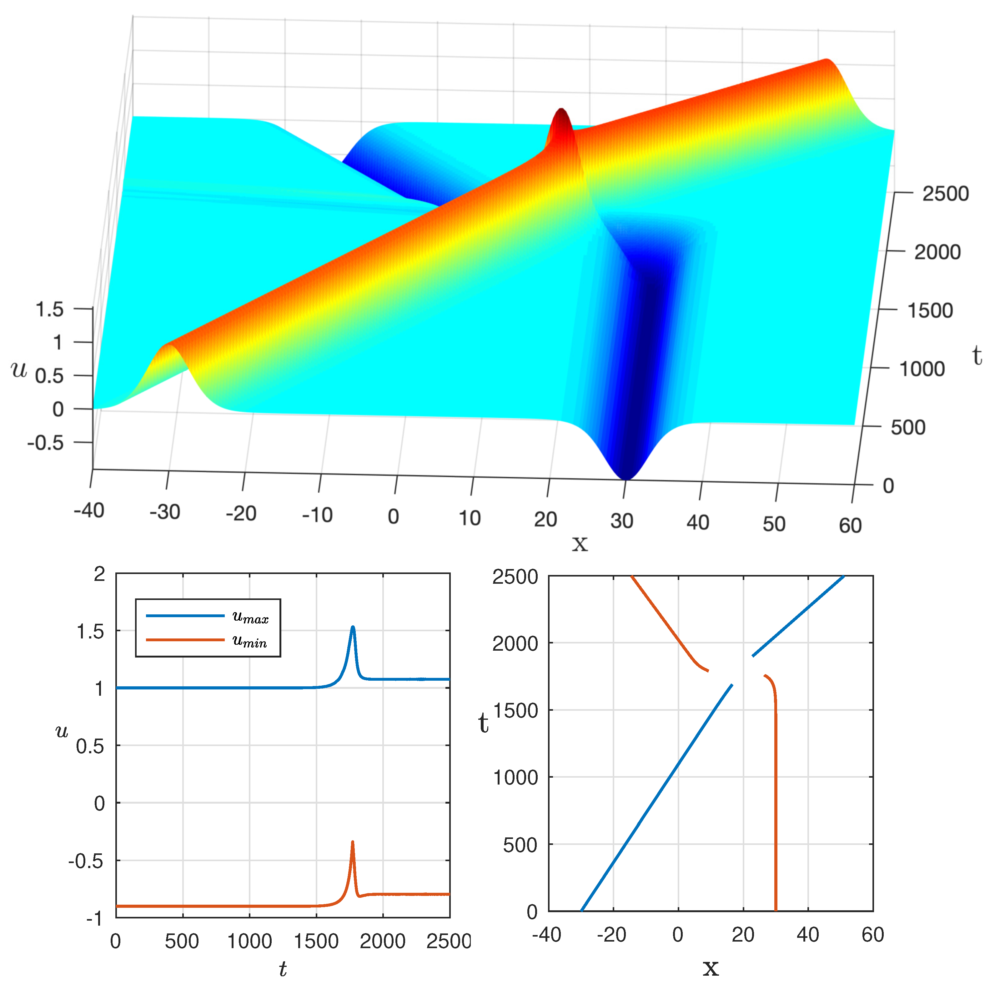
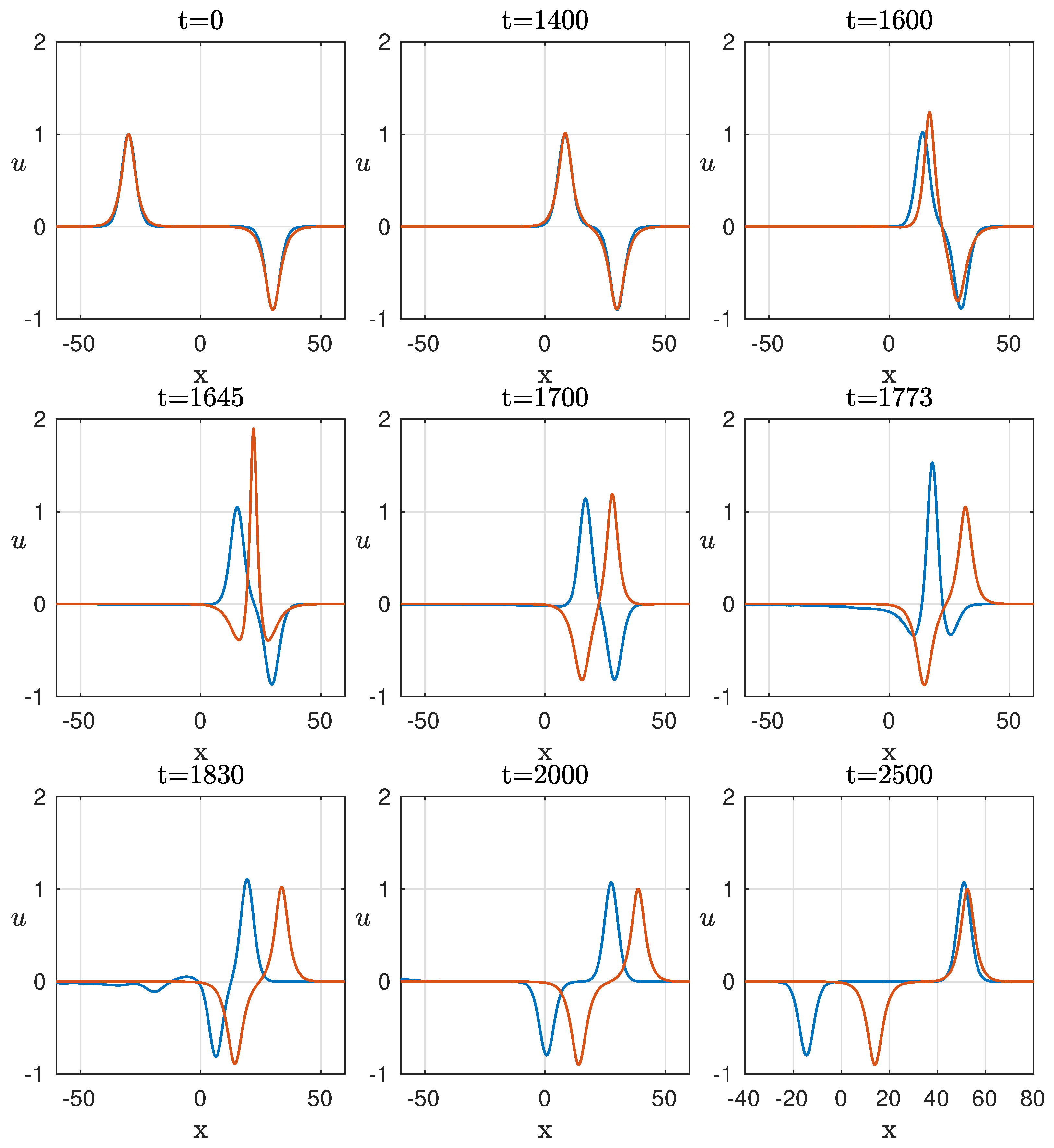
The properties of pair soliton interactions can be found in Figure 1. The bottom of this figure (left plot) demonstrates the evolution of the maximum of the wave field. It can be clearly seen that before interaction, the value of is equal to the value of the amplitude of the largest soliton; at the moment of interaction, it increases up to the value 1.53; however, after the separation, it does not return to its original value and remains at the level of 1.09. This means that a positive soliton increases its energy after the soliton collision. Consequently, the negative one loses its energy as is clearly seen in Figure 1 (bottom left), where the value increases after the soliton interaction and becomes equal to $-0.8$. There is no radiation that attenuates both solitons. In comparison with the integrable mKdV case, it is an inelastic collision with energy transfer from smaller to larger soliton. Thus, it can play a dramatic role in the soliton gas, when the energy concentrates in the biggest soliton which grows with time. It can be considered a new mechanism of rogue wave generation due to non-integrability. In fact, when the solitons have the same polarity [26], the dynamics of the wave field resemble the KdV-collisions except for the small radiation produced during the collision. In other words, the amplitudes are almost conserved.

Another intriguing finding is that the angle formed with the positive axis Ox and the soliton trajectory changes after the collisions (Figure 1, bottom right). For instance, the change for the negative soliton is ${90}^{\circ }-{103}^{\circ }=-{13}^{\circ }$, while for the positive soliton it is ${88}^{\circ }-{87}^{\circ }=1^{\circ }$. There is a big difference in comparison with the mKdV equation where only a phase shift occurs after the collision and the trajectories have the same angle.

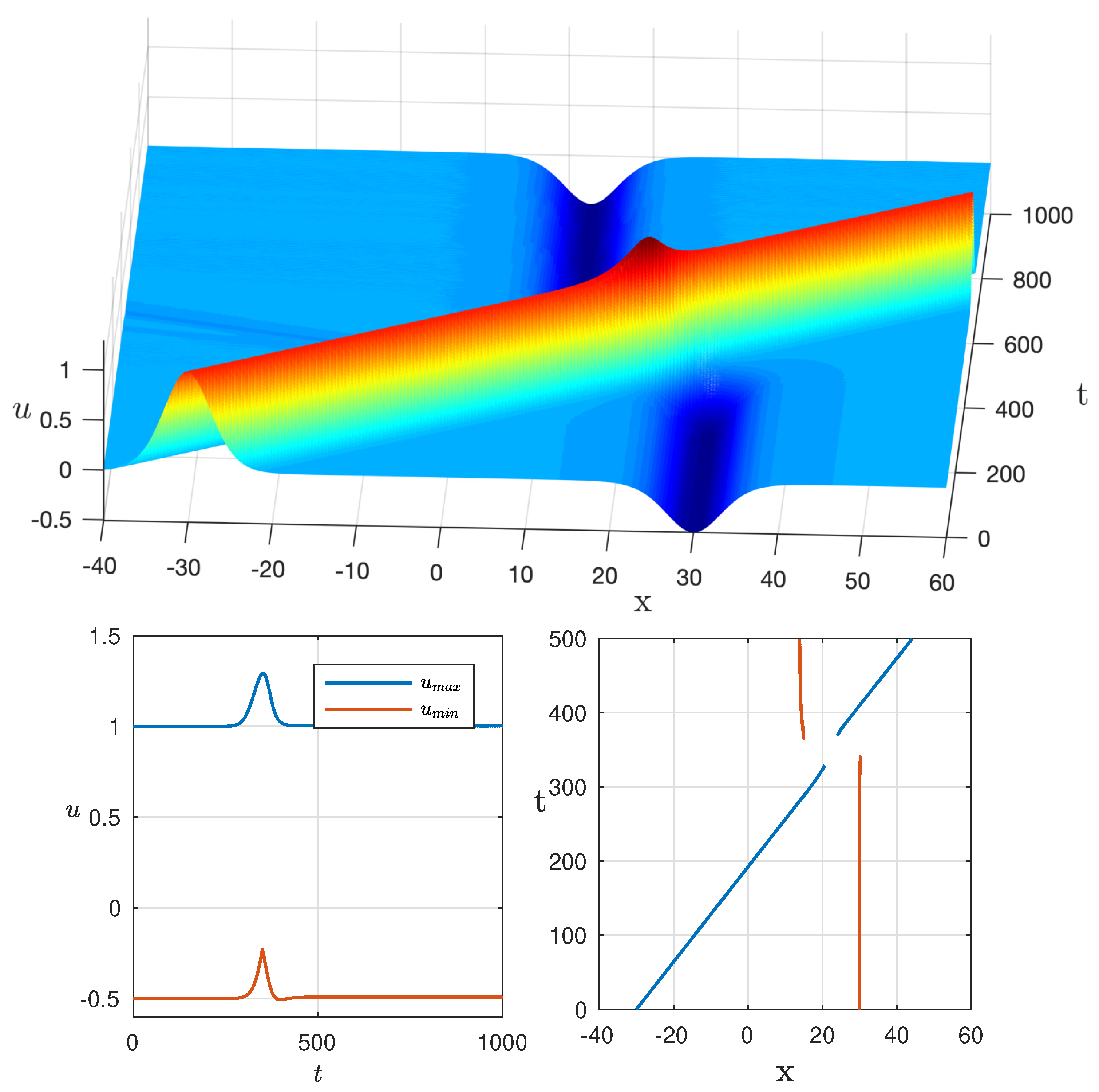
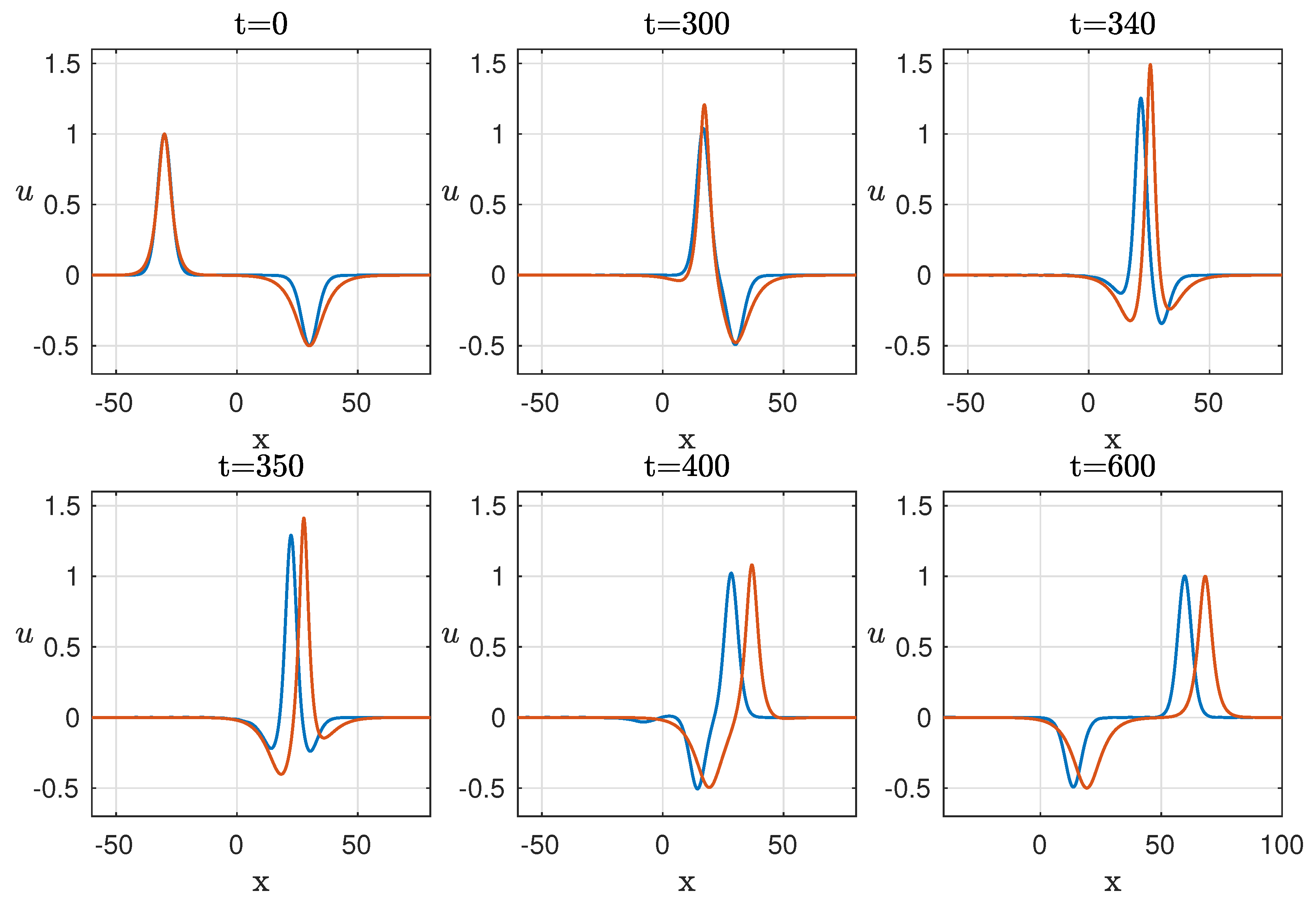
The features of soliton interactions depend a lot on the amplitudes of the solitons. Another example of pair soliton interactions is presented in Figure 2. Here, the value almost returns to its original value, and the angle between the positive axis Ox and the soliton trajectory does not change after the collisions. The value also restores after the solitons become separated.

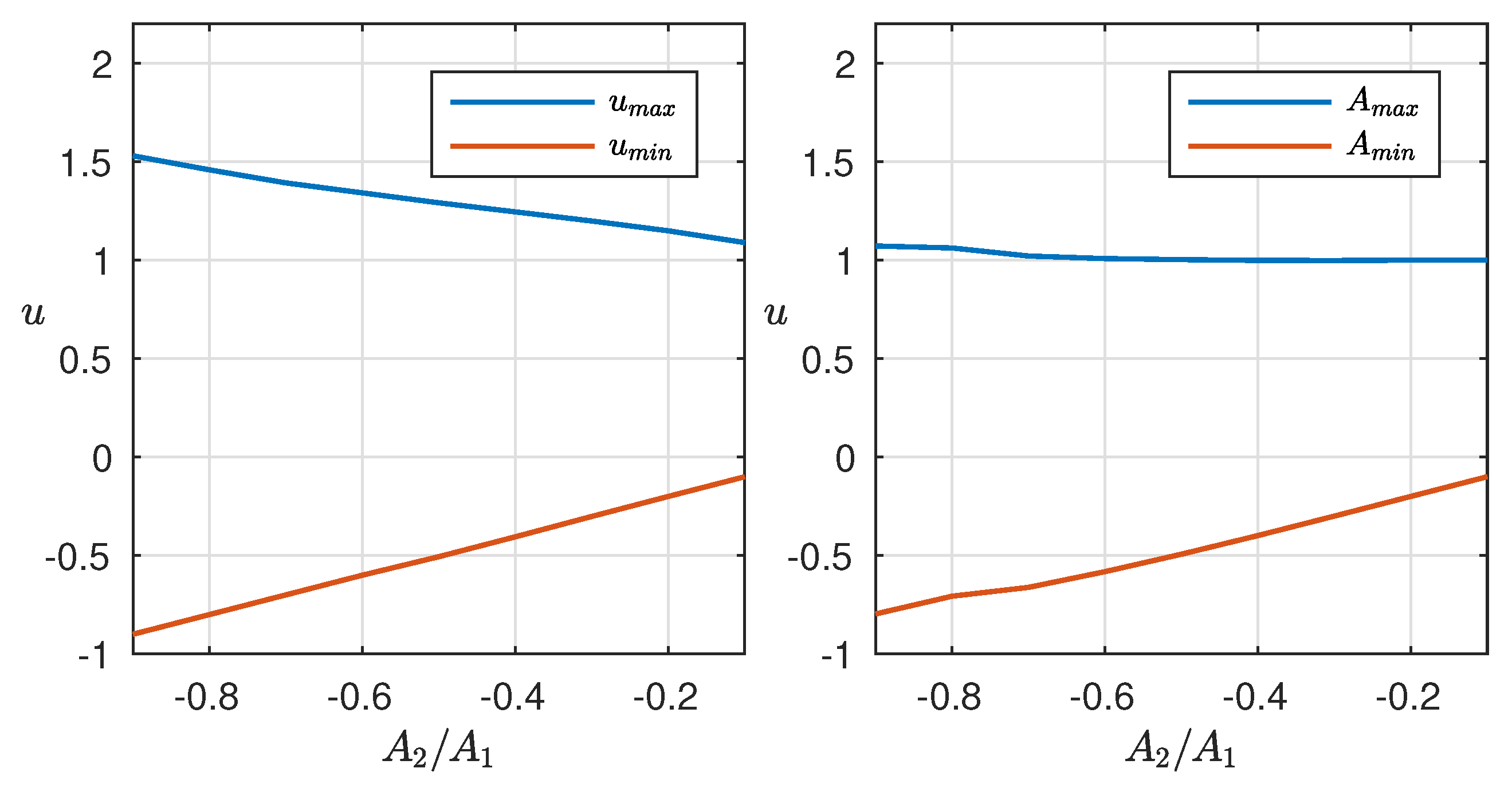
To study the dependence of extrema (maximum and minimum) of wave fields against the ratio of the amplitudes of the interacted solitons, as well as the values of amplitudes of the largest and smallest solitons after the soliton interaction, Figure 3 is analyzed. The amplitude of the largest soliton before the soliton collision was kept constant and equal to 1. The amplitude of the second soliton was changed from $-0.9$ to $-0.1$. It is observed that the minimum of the wave field for all considered ratios $A_2/A_1$ is equal to the amplitude of the smallest soliton and does not fall below this value over time. Thus, the straight red line can be seen in the left plot of Figure 3. The value of $u_{min}$ before and after the soliton interaction is not the same for all ratios $A_2/A_1$. This difference can be seen for amplitudes $A_2$ less than $-0.7$ (see red line on the right plot of Figure 3). This means that the negative soliton transfers part of its energy to the positive one only when their amplitudes are comparable in modulus. Accordingly, this effect does not appear when the amplitude of the negative soliton is considerably smaller than the amplitude of the large positive soliton. A similar conclusion can be made for the wave field maxima: the amplitude of the largest soliton after the soliton interaction exceeds its initial value (which is equal to 1) only for ratio $|A_2/A_1|$ bigger than $0.7$.

4. Comparison of the Process of the Soliton Interaction within the Schamel and the mKdV Equation

In the present section, the qualitative differences between the interaction of bipolar solitons within the non-integrable Schamel equation and integrable modified Korteweg-de Vries equation are analyzed.

The mKdV equation

$$u_t+u^2{u}_x+u_{xxx}=0.$$

(4)

also admits solitary waves as solutions described by the formulas

$$u(x,t)=asech(\left(k(x-ct)\right),\mathrm{where}v=\frac{a^2}{6}\mathrm{and}k=\sqrt{\frac{a^2}{6}}.$$

(5)

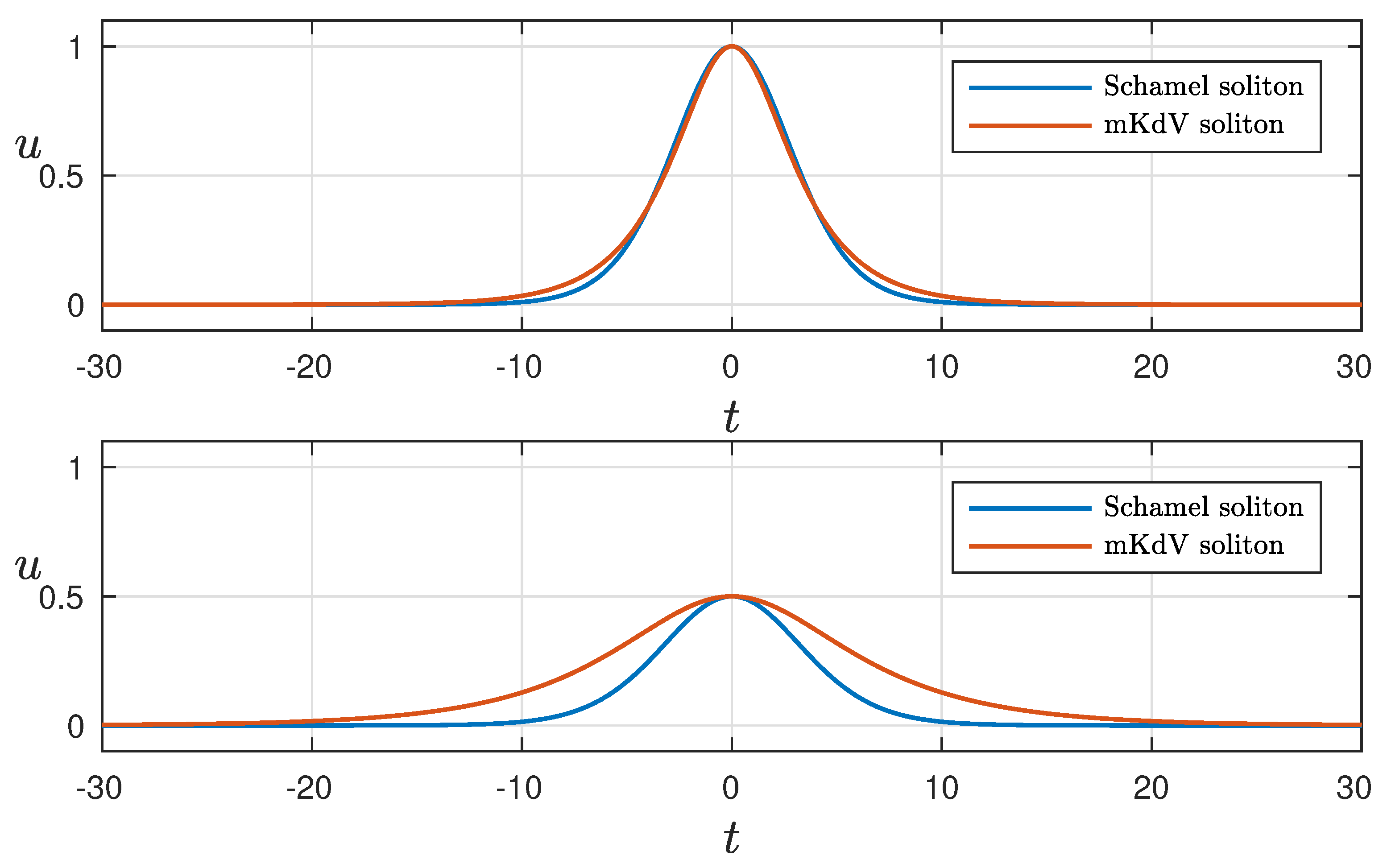
The soliton solutions of the Schamel equation are much narrower than the mKdV solitons with small amplitudes (Figure 4). Large solitons within the Schamel equation are a bit wider at the top of the soliton and narrower at the bottom in comparison with the mKdV solitons. Schamel solitons propagate faster than mKdV ones. These differences in shapes and velocities contribute to the difference in the interaction processes of solitons.

The process of two soliton interactions in an integrable mKdV model and non-integrable Schamel equation is presented in Figure 5 and Figure 6 for the simulations presented in Figure 1, and Figure 2 correspondingly. The interaction of bipolar solitons leads to an increase in the amplitude of the resulting impulse. However, within the mKdV model, the resulting amplitude presents the linear superposition of the modules of amplitudes of the initial solitons. The amplitude of the resulting impulse within the Schamel equation is less due to the additional radiation that occurs because of the non-integrability of this equation and the inelastic interaction of solitons. Also, in the mKdV model, the interacting solitons restored their shapes and amplitudes after the interaction, and the biggest wave which can form in the soliton gas has an amplitude equal to the sum of all solitons; this scenario requires very specific soliton phases and order of solitons [19,20]. In the framework of the Schamel equation, when solitons have close amplitudes by modulus (Figure 5), the scenario, on the one hand, is less extreme than the mKdV case because the resulting impulse is less than in the mKdV case. On the other hand, the amplitude of the largest soliton increases after the interaction. This may lead to the consumption of the energy of the largest soliton in soliton gas and, as a result, it may be considered a new mechanism of a freak or rogue wave formation due to the non-integrable effects. When the initial amplitudes of the solitons significantly differ from each other, the resulting impulse in the Schamel equation is again less than in the mKdV case, but not significantly, because the non-integrable radiation is small in this case (Figure 6). Moreover, after the interaction, the solitons have similar shapes as they had before the interaction.

Figure 5 and Figure 6 are plotted in the Schamel time, and the corresponding mKdV time is computed as

$$t_m=\frac{c_1-c_2}{v_1-v_2}.$$

(6)

Here, $c_1$ represents the positive Schamel soliton speed, while $c_2$ corresponds to the negative Schamel soliton speed. Similarly, $v_1$ denotes the speed of positive mKdV solitons, and $v_2$ represents the speed of negative mKdV solitons.

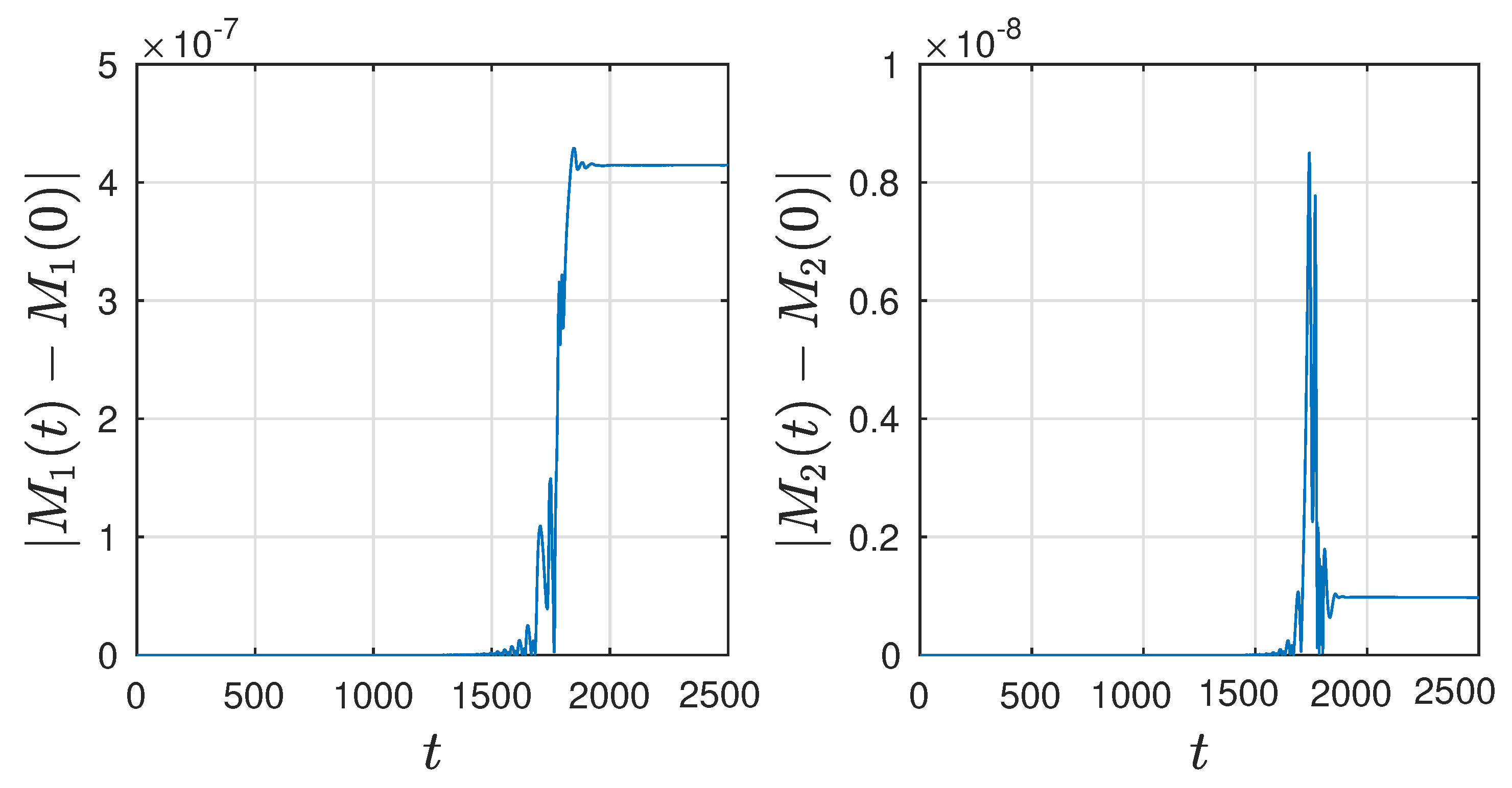
5. Moments of the Wave Fields

With the aim of understanding the contribution and the influence of pair interactions on the statistical moments of the wave field, the following integrals that correspond to four statistical moments were studied

$$M_n\left(t\right)={\int }_{-\infty }^{+\infty }{u}^n(x,t),\mathrm{for}n=1,2,3,4.$$

(7)

The first invariant $(n=1)$ is known as the Casimir invariant or the mass invariant. It characterizes the mass or the total “amount" of the wave field at any given time t. The second invariant $(n=2)$ is the momentum invariant. These invariants play a crucial role in evaluating the accuracy and reliability of numerical methods employed to solve the Schamel Equation (1). Their evolution within the Schamel equation is presented in Figure 7. It can be seen that the accuracy of the calculations is quite high, and the first and second integrals are preserved with an accuracy equal to ${10}^{-7}$ and ${10}^{-8}$.

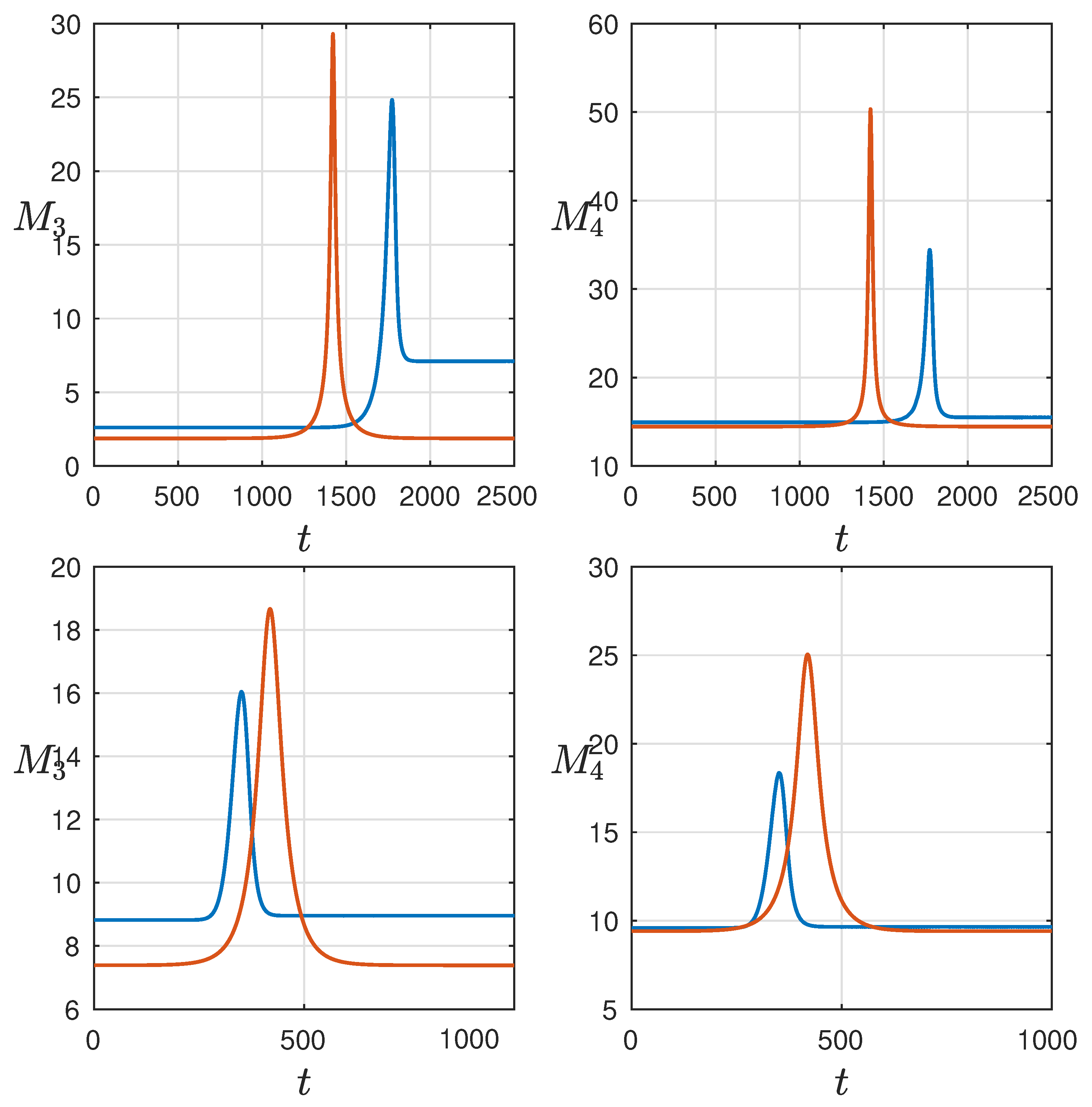
The third and fourth moments corresponding to the skewness and the kurtosis in the theory of turbulence vary in time and change their values during the soliton interaction. Their evolution and comparison for the two equations are shown in Figure 8 (top plot—in case of the simulation displayed in Figure 1) (bottom plot—in case of the simulation displayed in Figure 2). These moments increase in the moment of soliton interactions due to the increase in amplitude of the resulting impulse. The peaks of the moments are predictably higher within the mKdV equation than in the Schamel equation because the growth of impulses is larger in the mKdV equation as was shown in the previous section. By analogy with the maxima of wave fields, in the integrable mKdV equation, due to elastic soliton interactions, the values of the third and fourth moments before and after the interaction are identical. The same conclusion can be made for the Schamel equation in case of large differences in amplitudes of interacted solitons. The radiation due to the non-integrability of this equation is small enough. However, when the amplitudes of solitons are close in modulus ($A_2/A_1$ is bigger than 0.7), the value of the moments after the interaction becomes bigger than before the interaction. This means that in the case of the mKdV soliton interaction, the amplitudes of interacted solitons are higher than in the Schamel case. However, if in the Schamel equation, a large time of evolution of the wave field consisting of a large number of solitons is considered, the accumulation of energy in large solitons can contribute to the emergence of unexpectedly large waves in the system. Thus, non-integrability can be considered as a factor provoking the rogue wave formation.

6. Conclusions

We conducted an investigation into the collision dynamics of two solitons with different polarities, an essential aspect of soliton turbulence. This study involved numerical simulations using the non-integrable Schamel equation, and we compared the results to those obtained from the modified Korteweg-de Vries (mKdV) equation. Our findings revealed that when the amplitudes of the two solitons significantly differ in magnitude, the behavior of bipolar soliton interactions closely resembles that of the mKdV equation. In this scenario, despite the inelastic nature of soliton interaction, minimal radiation is generated within the Schamel equation. However, when the soliton amplitudes are close in magnitude, a distinctive effect emerges during the bipolar soliton interaction. Specifically, the amplitude of the resultant impulse increases, but it remains less than the sum of the soliton amplitudes prior to their interaction. Notably, in the case of close-magnitude amplitudes, the smaller soliton transfers a portion of its energy to the larger one. Consequently, the larger soliton amplitude increases while the smaller soliton amplitude decreases compared to their initial values. This phenomenon becomes especially pronounced in scenarios involving the interaction of bipolar solitons with similar amplitudes. As a result, large solitons have the potential to accumulate additional energy. This observation holds particular significance in the context of soliton turbulence or soliton gas, where a multitude of solitons interact repeatedly within the system.

Previously, it was shown that in the integrable KdV-like models, the bipolar soliton interactions can be a mechanism of rogue wave formation since the optimal focusing promotes the formation of the wave with an amplitude equal to the sum of amplitudes of interacted solitons even if their number is bigger than two. Within the Schamel equation, this effect is less pronounced due to the non-integrable radiation that occurs after the interaction. However, the energy accumulation in the largest solitons may contribute to the rogue wave formation in the case of long-term wave dynamics.