Article

Aggregation Methods Based on Quality Model Assessment for Federated Learning Applications: Overview and Comparative Analysis

Department of Automatic Control and Applied Informatics, “Gheorghe Asachi” Technical University of Iasi, 700050 Iasi, Romania
*
Author to whom correspondence should be addressed.
Mathematics 2023, 11(22), 4610; https://doi.org/10.3390/math11224610
Submission received: 10 October 2023 / Revised: 26 October 2023 / Accepted: 7 November 2023 / Published: 10 November 2023
(This article belongs to the Special Issue Artificial Intelligence and Data Science)

Abstract

:
Federated learning (FL) offers the possibility of collaboration between multiple devices while maintaining data confidentiality, as required by the General Data Protection Regulation (GDPR). Though FL can keep local data private, it may encounter problems when dealing with non-independent and identically distributed data (non-IID), insufficient local training samples or cyber-attacks. This paper introduces algorithms that can provide a reliable aggregation of the global model by investigating the accuracy of models received from clients. This allows reducing the influence of less confident nodes, who were potentially attacked or unable to perform successful training. The analysis includes the proposed FedAcc and FedAccSize algorithms, together with their new extension based on the Lasso regression, FedLasso. FedAcc and FedAccSize set the confidence in each client based only on local models’ accuracy, while FedLasso exploits additional details related to predictions, like predicted class probabilities, to support a refined aggregation. The ability of the proposed algorithms to protect against intruders or underperforming clients is demonstrated experimentally using testing scenarios involving independent and identically distributed (IID) data as well as non-IID data. The comparison with the established FedAvg and FedAvgM algorithms shows that exploiting the quality of the client models is essential for reliable aggregation, which enables rapid and robust improvement in the global model.
MSC:
68T07; 68W15

1. Introduction

Federated learning (FL) [1,2,3] is a widely used and appealing research approach that generates a global model by handling private data sets that are spread out among different clients. The design method is built using the principle of privacy-preserving data to respect the General Data Protection Regulation (GDPR). Each client possesses a unique training data set kept locally. Accordingly, each client calculates an update based on the current global model maintained by the server and only transmits this update. This technique holds great promise for several machine learning applications which use sensitive user information to train their local models—hospital data [4,5], web social platforms’ data [6], drivers’ data [7], etc.—because they allow the organizations to collaborate without explicitly sharing user data with a central location. As the training effort is distributed to multiple clients, FL becomes suitable for complex learning tasks involving big geographically dispersed training data sets, which could be acquired by autonomous sensing or data collection techniques in local protected data sets. For example, the authors of [8] presented an application for predicting or maintaining a radio environment map where unlicensed users can locally use some frequency bands based on the spectrum occupation in a given area. Another example detailed in [9] is related to object detection for a vehicular-to-everything (V2X) network, in which the authors proposed a cooperative sensing methodology.
The authors of [10] introduced three categories for FL based on the types of data that are kept private or shared by clients: horizontal federated learning (HFL) [11], vertical federated learning (VFL) [12], and federated transfer learning (FTL). HFL is suitable for cases in which clients share the same feature space, but their samples are private, while VFL is used when clients need different feature spaces and share the same samples, with the encryption and paring of samples being carried out by a third-party entity. Lastly, FTL applies to data sets that have different features and instances [13]. For each category, a different design should be considered [10]. However, for all architectures, FL maintains data confidentiality and privacy specifically in the context of GDPR compliance because the communication between the server and clients refers to the parameters of the model and not to the raw training data stored by each client. The parameters of the model are not targeted by the GDPR and can be shared between nodes without privacy constraints. Any other additional information is communicated only with client agreement as in the case of VFL, where the encryption and pairing of samples are performed by an authorized third-party entity without allowing any client to access the raw data of any other client.
Depending on the communication allowed between nodes, FL methods can be grouped into centralized and decentralized methods [14]. Centralized federated learning (CFL) is a commonly used architecture that includes a server and allows client–server interactions [1,15], while the decentralized federated learning (DFL) structure does not contain a centralized node and allows the clients to communicate directly with each other [16]. In this paper, the focus is on the HFL and CFL structure, which is also named sample-based federated learning. HFL and CFL can be customized for each problem, but the root concept is the same for all algorithms, as shown in Figure 1. The server is the primary actor in this process; it sends an initial model to the clients and then, at every communication round, receives the updated local models, aggregates these models into the global model, and resends the resulting global model to the clients for further improvements.
HFL is confronted with several challenges in real-world applications because the clients do not necessarily have the same number of training samples or the same distribution of training data sets. If the distribution of the local training data set does not illustrate the overall distribution of data across all nodes, then the local training is biased and likely exposed to generate an underperforming model. Another crucial concern is posed by clients with malicious intent who may attempt to manipulate the performance of the server. Such clients should be regarded as intruders or attackers in the process [17]. Also, problems may appear when the communication paths between the server and participating clients are affected by various disturbances [18]. Based on this, FL is facing challenges that researchers are currently analyzing, such as (1) heterogeneity of data and devices, where connected clients may have different distributions of local training data and use different types of devices, which can lead to a decrease in the overall performance of the central model [19,20]; (2) vulnerability of the server, where there is a possibility that the global model may be vulnerable to certain attacks or low-quality client data [21]; and (3) efficiency of communication, where the FL approach involves the communication between a server and connected clients, which can lead to a limited communication bandwidth to transfer local updates [22,23]. In this context, the aggregation should limit the influence of poor clients. This aspect is essential for effective FL because any damage to the global model is propagated throughout the entire network in subsequent communication rounds when the global model is sent to clients for additional training.
The flow of HFL assumes that local and global models have the same architecture. Typically, the server performs a parameter-level weighted linear aggregation. This simplified approach is adopted even for nonlinear models, assuming that only minor updates are handled at each communication round. The authors of [24] highlighted that the effects of artificial noise disturbing the parameters of the local models also depends on the structure of the model. This noise can be induced by the aggregation of intruded or underperforming clients. In this regard, in [24], it was shown that the influence of intruded clients on the accuracy of the global model is much stronger in the case of convolutional neural networks than in the case of multilayer perceptrons. The impact of each local model can be adjusted by the weighting procedure, which may become key to processing non-IID data and protecting the global model against less effective clients. To ensure an unbiased and effective aggregation of local models, the weighting procedure should take into account that the quality of the local models is influenced by many factors, from the distribution of local training data sets to the local configuration of the training procedure or cyber-attacks. Browsing through potential issues and evaluating their impact is a highly difficult task. However, as will be discussed later, comprehensive fault diagnosis is not necessary, and aggregation can directly exploit quality indicators (like accuracy) that highlight any important issue related to the local models. It is important to note that it is more important for the aggregation method to detect poor clients than to isolate the cause that generated this behavior.
In this context, this paper introduces FL methods that evaluate the performance of the local models to support a reliable aggregation. The proposed algorithms use the average accuracy of local models as a threshold to avoid integrating data from untrustworthy or underperforming clients. In addition, the influence of each client relies on the performance of its local model. The weights used for the linear aggregation of the local models depend on their accuracy or are obtained via Lasso regression using refined information, like predicted class probabilities. The comparative analysis investigates some of the main challenges of the FL approach. First, the work involves examining the effects of data heterogeneity on the global model. This includes the unequal distribution of data among clients and the usage of non-IID data. The testing scenarios also monitor the actions of negative clients who may attempt to compromise the global model. This involves simulating the presence of intruders during the learning process. The most important contributions of our work are mentioned below:
  • A detailed discussion of the benefits and limitations resulting from using local models’ accuracy in the aggregation step with a focus on our methods: FedAcc and FedAccSize [25];
  • The design of a new aggregation method, FedLasso, which enhances the assessment of local models’ quality by applying Lasso regression, where the resulting Lasso coefficients are exploited for parameter-level aggregation;
  • An experimental analysis of the aforementioned methods in comparison with two algorithms widely recommended in the literature (FedAvg [1] and FedAvgM [26]), where the testing scenarios simulate intruded or underperforming clients for both IID and non-IID data.
The rest of this paper is organized as follows. Section 2 offers an overview of related works, where the focus is on aggregation techniques. Then, Section 3 presents two averaging algorithms which are among the most popular in FL to set a reference for our developments. The algorithms using the quality of local models for a refined aggregation are introduced in Section 4, and the experimental scenario and results are detailed in Section 5. At the end, some conclusions are provided.

2. Related Works

FL training methods have evolved from the original federated averaging (FedAvg) algorithm [1]. FedAvg uses a weighted average of the local model updates to establish the modifications of the global model at every communication round. Every client stores a local data set that is not shared with the other clients or the server. The local models are trained using the stochastic gradient descent (SGD) method. The relevance of clients participating in aggregation relies only on the ratio of local training samples from the total amount of data accessed by the active clients. The algorithm thus cannot consider clients with different distributions of local data or with ineffective training. However, since it was introduced, FedAvg has been preferred in many works due to its simplicity and is still a standard approach for IID data.
An improved version of FedAvg, named federated averaging with server momentum (FedAvgM), was introduced in [26]. FedAvgM implements a momentum technique at the server level. More precisely, the variations in the global model are set while considering a linear combination between the variation obtained in the previous communication round and the variation resulting from current local model updates. This aggregation method favors a stable and fast learning process, but its performance remains limited in the case of non-IID data. Another interesting extension of FedAvg is the federated framework for heterogeneous networks, called FedProx [15]. This algorithm uses a supplementary proximal term in the local loss function. The extra term is equal to the norm of model parameter variation, and hence the minimization of the loss function performed during training implicitly promotes local updates close to zero, which are suitable for the aggregation of nonlinear models. The clients provide γ -inexact local solutions to deal with heterogeneous training efforts and non-IID data. However, the protection against attacks and inconvenient local data sets remains limited. In [27], the authors proposed a method for evaluating the trustworthiness of clients using the history of interactions with each user. The main assumption is that the server can detect the anomalies of local models. Recent and direct interactions have the biggest influence on the trustworthiness scores. However, the procedure can exploit recommendations received from other servers and long-term recordings as well. The most reliable and trustworthy clients are selected for aggregation of the global model. The detection of anomalies implicitly includes an evaluation of the local models and could be carried out using their accuracy, as proposed in our work. The authors of [8] built an FL system with three clients, including a negative client working with an incorrectly labeled data set and a client responsible for evaluating the local models. Thus, the evaluator helps the server in the aggregation process to ignore models under a defined threshold. The authors highlighted that some spectrum opportunities can be lost under this approach when full protection is applied. An important benefit of the method could be the ability to define a threshold based on the quality of the models, as suggested in our paper.
A different communication flow between server and clients is suggested by CO-OP [28]. Unlike FedAvg, CO-OP integrates a local model into the global one immediately after it is received by the server without waiting for other responses from clients. The clients receive the updated global model and can decide if the new parameters are imported or if they continue the ongoing local training process. The algorithm uses protection against outdated or overactive clients to avoid the integration of improper local models. However, as the global model can be updated by a single client, its optimization can become unstable and exposed to attacks and underperforming clients. InfeMo [29] combines CO-OP and FedAvg. The server communicates with the clients in several rounds, but only clients with an appropriate maturity are accepted for aggregation, and clients can refuse the importation of the global model to continue their ongoing training. The difficulty remains in providing a proper transfer of learning between clients, although they can decline the global model.
Regardless of the performance of the local learning process, the aggregation performed at the parameter level cannot guarantee an improvement in the global model when this model is nonlinear. In this context, federated matched averaging (FedMA) [30] assumes a layer-based model structure, and at each step, it aggregates the updates corresponding to a single layer of the model. The clients receive the modified parameters and apply the training process for the next layer to accommodate previous modifications in the local nonlinear model. This approach looks for similarities between the subsets of the local parameters and extends the global model to integrate local components corresponding to unmatched subsets. However, the aggregation is vulnerable to intruders and worse-performing clients, which can trigger undesired expansion of the global model. The similarity of clients is also investigated with the similarity-guided model-based aggregation method FedSim [31]. To enhance the performance of the global model, this method clusters the clients with respect to the resulting gradients and then performs an intra-cluster aggregation followed by a global aggregation across all clusters.
Helpful ideas for reducing the influence of less-adapted models can be obtained from the methods proposed in real-time systems to solve Byzantine attacks [32]. This includes ignoring outlier updates before weighted averaging or using the median instead of the weighted average. In addition, the clients could be protected against improper modifications received from the server. For example, if the global model is much worse than the available local one, then its parameters are not imported by the client to limit the propagation of attacks or underperforming aggregation. Unfortunately, without having information about the distribution of data from the other nodes, these protection techniques can also limit the transfer of knowledge between clients, thus impeding the model from accommodating other data and improving its generalization capability.
The authors of [32] argued that the detection of intruders in FL approaches can be guaranteed only if a relaxation of data privacy constraints is accepted. In line with this idea, the authors of [33] used a central validation set to filter out adversarial and poor clients. The differences between the best and the rest of the models, computed in terms of accuracy, are exploited to prevent corruption of the global model by intruded clients. Another interesting approach based on generative adversarial networks (GANs) was suggested in [21]. From random noise input, the GAN creates fake samples with the same distribution as the real data, which are used to simulate backdoor attacks. The analysis shows that no guarantee can be given to prevent attacks without assessing the quality of the local models. In extension, our work includes aggregation techniques that refine the contribution of clients to the global model based on the quality of the local models. As detailed in the next sections, this mitigates the risk of using the local models sent by intruders or clients with improper training performance.
Numerous aggregation approaches have also been proposed to combine models designed for different modalities or data sets, such as Bayesian aggregation [34,35]. Unlike the common configuration of HFL, most of these methods consider an output-level aggregation and expand the structure of available basic component models to integrate them into the global one. They also use regularization techniques to avoid numerical problems and overfitting caused by increased model complexity. The least absolute shrinkage and selection operator (Lasso) is frequently used for regression models to improve accuracy and preserve simple, easy-to-interpret architectures [36,37,38]. An interesting method based on Lasso regression is presented in [39]. This aggregation strategy, called FedFit, updates the global model using two main processes: (1) parameter compression at the client level, considering the same base for all clients, and (2) parameter reconstruction on the server using Lasso regression. As the parameters of the model are exchanged between the server and clients only after compression, the communication load is substantially reduced. In our approach, Lasso regression is considered for another purpose. The Lasso coefficients are used to calculate the weights associated with clients for aggregation of the models at the parameter level. The aggregation is discussed both for regression and classification problems.

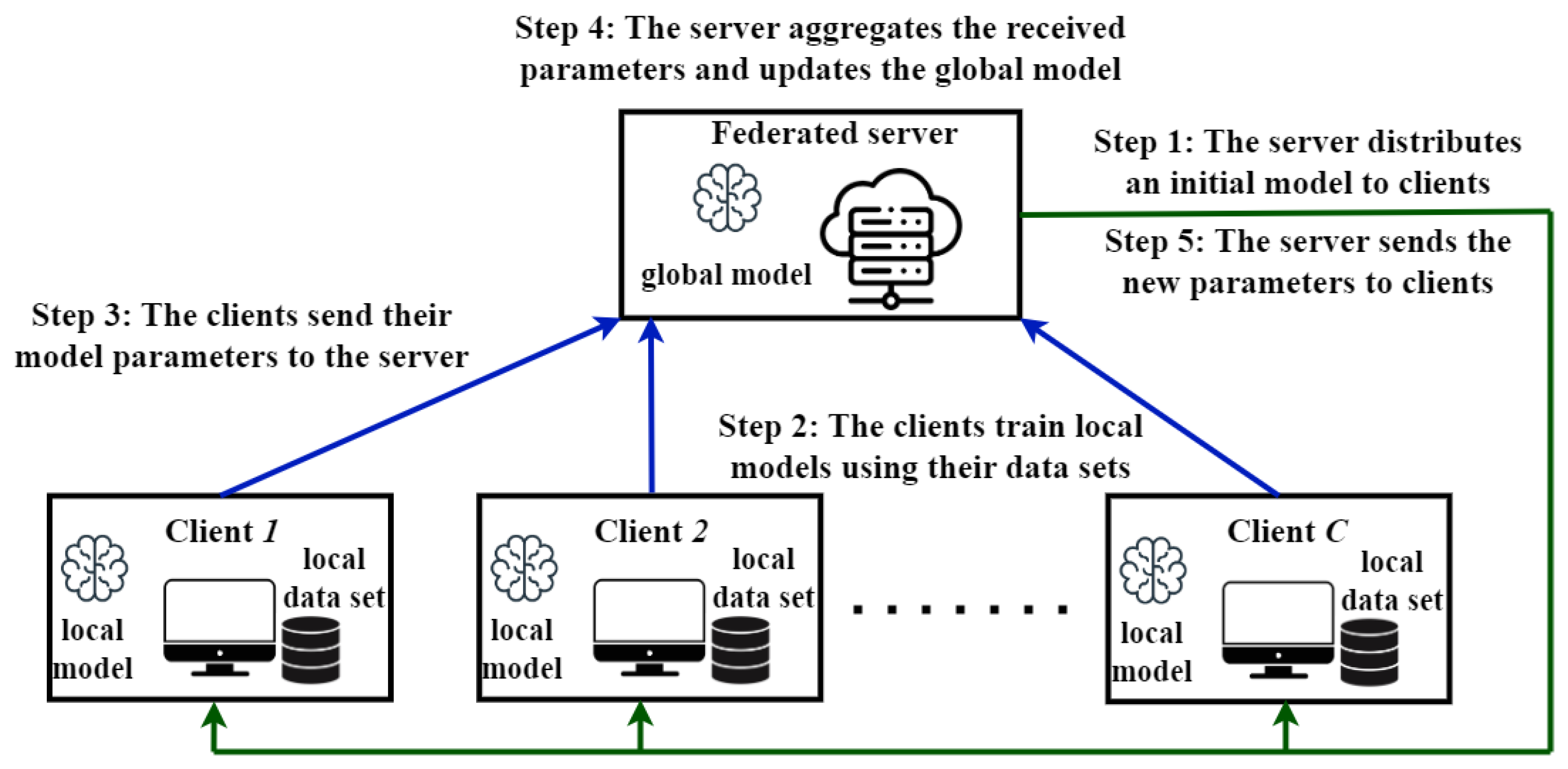
3. Aggregation of Local Models in Federated Learning

To provide a background for the proposed methods, this section discusses two of the most recommended algorithms in the literature, namely FedAvg [1] and FedAvgM [26]. They will also be used as a reference for the performed experimental analysis.
For simplicity, all notations are listed in Table 1. Being HFL methods, FedAvg and FedAvgM have a central component, the server, and C clients who collaborate for training the global model stored on the server. The parameters of the global model are obtained as a result of communication between the server and clients, which exchange information about the model parameters during some communication rounds. In each round of communication, active clients are checked, and they are allowed to participate in the learning process. As mentioned before, FedAvg and FedAvgM consider a linear aggregation of the local models, where the weights associated with clients rely on the ratio of training samples they use. As an extension to FedAvg, FedAvgM performs the aggregation with momentum to ensure more stable learning for the global model.
Algorithm 1 depicts the detailed pseudo-code of FedAvg and FedAvgM. Every client j who participates during the rth round of communication follows two main steps: initialization and training. Initialization means that the client j receives from the server the parameters of the global model ( ϕ r 1 ) and copies these parameters into its local model. Then, the client trains its local model for E j epochs using the SGD method:
ϕ j ( k ) = ϕ j ( k 1 ) η j J ϕ j ( ϕ j ( k 1 ) , D j ) ,
where ϕ j ( 0 ) = ϕ r 1 and k { 1 , , E j } . The resulting parameters, ϕ r j = ϕ j ( E j ) , or the resulting updates, Δ ϕ r j = ϕ j ( E j ) ϕ r 1 , are passed to the server for the next aggregation. The server collects the updates obtained by all active clients, computes the weights associated with them, and updates the global model:
ϕ r = ϕ r 1 + j S r w r j · Δ ϕ r j = j S r w r j · ϕ r j ,
where
w r j = | D j | p S r | D p | .
As specified above, the weights rely on the size of the local training data sets. The highest confidence is associated with the active client having the largest training data set. According to Equation (3), the result is that j S r w r j = 1 and w r j [ 0 , 1 ] , j S r . Similar weights are used by FedAvgM. This algorithm memorizes the previous update of the global model to implement momentum-based learning. The previous variation is combined with the current one to accelerate learning and diminish the risk of oscillations [26]:
ϕ r = ϕ r 1 + Δ ϕ r ,
where
Δ ϕ r = β Δ ϕ r 1 + j S r w r j · Δ ϕ r j , with β ( 0 , 1 ) .
Algorithm 1 Aggregation methods: FedAvg and FedAvgM
  1:
Server steps:
  2:
global model initialization—with parameters ϕ 0
  3:
for  r 1 to R do:
  4:
      send the current global model ( ϕ r 1 ) to all clients
  5:
      for each active client j S r  do:
  6:
           receive updates from this client: Δ ϕ r j ClientUpdate(j, ϕ r 1 , D j , η j , E j )
  7:
           compute w r j according to Equation (3)
  8:
      for each active client j S r  do:
  9:
           aggregate the updates from this client into the global model:
10:
             for FedAvg—using (2); for FedAvgM—using Equations (4) and (5)
11:
 
12:
procedure CLIENTUPDATE(j, ϕ r 1 , D j , η j , E j )
13:
      local model initialization—with parameters ϕ r 1
14:
      for  k 1 to E j  do:
15:
           compute ϕ j ( k ) using (1)
16:
      compute model update, Δ ϕ r j = ϕ j ( E j ) ϕ r 1
17:
      return model update, Δ ϕ r j

4. Aggregation Based on Local Models’ Quality Assessment

As previously mentioned, refined protection against intruders and underperforming clients can be obtained only if the server gathers information about the quality of incoming models. The detection of improper clients is important as they degrade the federated learning process. However, the analysis should consider that the clients might need different training efforts, depending on the distribution and size of their local training data sets. Clients who use diverse and large data sets could provide improper intermediary results, as they are involved in complex learning tasks. However, for the overall purpose, these clients are crucial for accommodating the global model to diverse data and providing improved generalization capabilities.
In this section, we propose aggregation methods that exploit the accuracy of the local models or refined information related to model predictions. This implicitly reveals potential problems related to data distribution, improper training, or intruders in support of a reliable aggregation. We first examine the two proposed methods, FedAcc and FedAccSize from [25], and then introduce a new method, FedLasso. All these algorithms eliminate poor clients and combine the remaining local models using weights which rely on their quality to ensure a reliable aggregation. As detailed in the next section, the main differences between these aggregation algorithms are related to the computation of the weights associated with the accepted clients.

4.1. Examination of FedAcc and FedAccSize

FedAcc and FedAccSize [25] were proposed to detect ineffective clients who can degrade the federated learning process in order to reduce their impact on the resulting global model. To this end, the algorithms exploit the local model accuracy to select the models accepted for the aggregation and to define the weights associated with accepted clients. The threshold for acceptance is the average accuracy of the active clients A c c ¯ r .
In the same way as FedAvg and FedAvgM, these two proposed methods use the initialization and training steps. The differences result from the protection mechanism implemented by the server against improper clients and how the weights are defined. For any active client j, during the rth communication round, an intermediary coefficient ψ r j is computed. For FedAcc, ψ r j relies on the local accuracy A c c r j to promote valuable models:
ψ r j = e A c c r j , if A c c r j A c c ¯ r 0 , otherwise
For FedAccSize, ψ r j relies on the local accuracy A c c r j and the size of the local training data set | D j | to promote models with good performance that learn from vast training data sets. These clients can gather valuable knowledge, but their training process might be long. The supplementary term introduced in FedAccSize permits increasing the corresponding weight from the early training stages:
ψ r j = e A c c r j · | D j | p S r | D p | , if A c c r j A c c ¯ r 0 , otherwise
For both algorithms, the coefficient is strictly positive for clients with above-average accuracy who are accepted later for aggregation. These coefficients are then normalized to obtain the weights used for aggregation:
w r j = ψ r j p S r ψ r p
This ensures null weights for the clients who should be ignored during aggregation. The resulting weights could be directly used in Equation (2) to produce the global model. The flow is summarized in Algorithm 2.
To evaluate the quality of the local models, the server could store a validation data set populated with samples received from clients for which a relaxation of data privacy constraints is accepted. This version is possible in many real applications and permits refined data distribution analysis. The validation data set could also be collected from other sources or artificially generated. In this case, its distribution should be verified in collaboration with clients. Another option consists of keeping local validation data and passing the local models between nodes for cooperative quality assessment. In this case, the FL system is fully aligned with the GDPR without additional agreements, but it should support increased communication between clients and is vulnerable to fake accuracy values sent by intruders.
The use of accuracy for refining the influence of clients on the global model is motivated by several aspects: (1) if assessed on a proper validation data set, the accuracy can set the reliance on clients and reveal local misconducted training, and (2) the accuracy can easily be evaluated with reasonable computational resources. However, the accuracy can hide several problems related to data set distribution, like the lack of balance between classes. To this end, the next subsection presents an extension of these two algorithms, which exploits refined information from the local models.   
Algorithm 2 Aggregation methods: FedAcc and FedAccSize
  1:
Server steps:
  2:
initialize the global model—with parameters ϕ 0
  3:
for  r 1 to R do:
  4:
     send the current global model, ϕ r 1 , to all clients
  5:
     initialize the average accuracy: A c c ¯ r 0
  6:
     initialize the total number of training samples used in this round: N r 0
  7:
     for each active client j S r  do:
  8:
          receive updates from this client: Δ ϕ r j ClientUpdate(j, ϕ r 1 , D j , η j , E j )
  9:
          compute the accuracy of the local model, A c c r j
10:
          add client’s contribution to the average accuracy: A c c ¯ r A c c ¯ r + A c c r j | S r |
11:
          add client’s contribution to the total number of training samples: N r N r + | D j |
12:
    for each active client j S r  do:
13:
          compute ψ r j : for FedAcc—using Equation (6); for FedAccSize—using Equation (7)
14:
    for each active client j S r  do:
15:
          compute w r j according to Equation (8)
16:
          aggregate the updates from this client into the global model using Equation (2)

4.2. Description of FedLasso

The newly proposed aggregation method, FedLasso, adopts the same special mechanism to eliminate improper clients from aggregation. But, unlike the previously specified algorithms, the weights are calculated using Lasso regularization.
Usually, Lasso regularization is applied in regression problems to improve the accuracy and interpretability of the resulting global model. The aggregation is solved at the output level by solving the following minimization problem
min L 0 , L 1 N n = 1 N ( y n L 0 x n T L ) 2 + α m = 1 M | L m | ,
to produce the aggregated model L 0 + x T L . Here, ( x n , y n ), with n = 1 , , N , defines the data set, where x n = [ x n 1 , , x n M ] T R M specifies the covariates, y n R specifies the target values, T indicates the transpose operator, L 0 is the constant term of the model, L = [ L 1 , , L M ] T gathers the Lasso coefficients, and α ( 0 , 1 ) .
Equation (9) could easily be extended to FL if aggregation at the output level is accepted and the model is configured for regression. In this case, the covariates correspond to the outputs of the local models evaluated on the validation data set for the active clients. As we are interested in performing a parameter-level aggregation, FedLasso uses a null intercept ( L 0 = 0 ) and defines the relevance of models based on the associated Lasso coefficients. Exactly as in the case of FedAcc and FedAccSize, only valuable clients with above-average accuracy are accepted for aggregation, which means that only these clients are taken into account for the minimization problem:
min L 1 N n = 1 N ( y n x n T L ) 2 + α m S r ˜ | L m | ,
where S r ˜ = { j S r | A c c r j A c c ¯ r } specifies the active clients with above-average performance. Here, | S r ˜ | = M C . As a result, the intermediary coefficients are
ψ r j = | L j | , if A c c r j A c c ¯ r 0 , otherwise
and the normalization indicated in Equation (8) is used to compute the weights.
The extension of FedLasso to classification problems is accomplished by using the predicted class probabilities as covariates and the target value of one for each validation sample. The model has Q outputs, with each one dedicated to a class as recommended for the classification approach. The class probabilities can be provided by the softmax layer included in the architecture of the model. If the model does not include a softmax layer, then the class probabilities can be obtained using a softmax transformation of the raw float outputs of the model according to the following equation:
( z n , i j ) = e z n , i j q = 1 Q e z n , q j ,
where z n , i j with i { 1 , , Q } , n { 1 , , N } indicates the ith raw output of the client j computed for the nth validation sample, Q specifies the number of classes, and ( z n , i j ) indicates the resulting output value. In Equation (12), the softmax function ensures that for any local sample n, the outputs of the local model z n , i j are mapped to positive values that can be interpreted as probabilities (i.e., ( z n , i j ) [ 0 , 1 ] , i { 1 , , Q } and i = 1 Q ( z n , i j ) = 1 ). Large, positive outputs correspond to large class probabilities. The larggest class probability indicates the class associated with the sample. To avoid poor conditioning and improve performance in the case of unbalanced data sets, the covariates can be designed as the mean predicted probabilities assigned to each class:
x i j = 1 | Ω i | n Ω i ( z n , i j ) ,
where Ω i { 1 , , N } is the subset of samples belonging to class i. This also permits applying Lasso regularization to covariates of a reduced dimension Q. The suggested computation steps are summarized in Algorithm 3. FedLasso results from Algorithm 2 by using this new procedure for the computation of intermediary coefficients instead of Equation (13). This means that the intermediary coefficients are computed using Equations (1013) instead of Equation (6) or (7).
Algorithm 3 Intermediary coefficients: FedLasso
1:
for each active client j S r  do:
2:
     for  i 1 to N do:
3:
           compute the predicted class probabilities according to Equation (12)
4:
     compute the values corresponding to this client in Lasso regression using Equation (13)
5:
apply Lasso regularization according to Equation (10), with clients sorted with respect to accuracy
6:
compute the intermediary coefficients ψ r j for all j S r according to Equation (11)

5. Experimental Design and Illustrative Results

The experiments were designed to provide a comprehensive framework for the comparative analysis of the algorithms described above. As elaborated upon in the next subsections, the testing scenarios were defined for classification problems and involved both IID and non-IID data, as well as artificially generated intruders. The comparison was performed between aggregation algorithms that investigate the quality of local models (FedAcc, FedAccSize [25], and FedLasso) and standard algorithms that take into account reduced information about the training environment (FedAvg [1] and FedAvgM [26]). In all cases, the clients and the server used the same structure for the model (i.e., a multilayer perception (MLP)), and aggregation was performed at the parameter level.

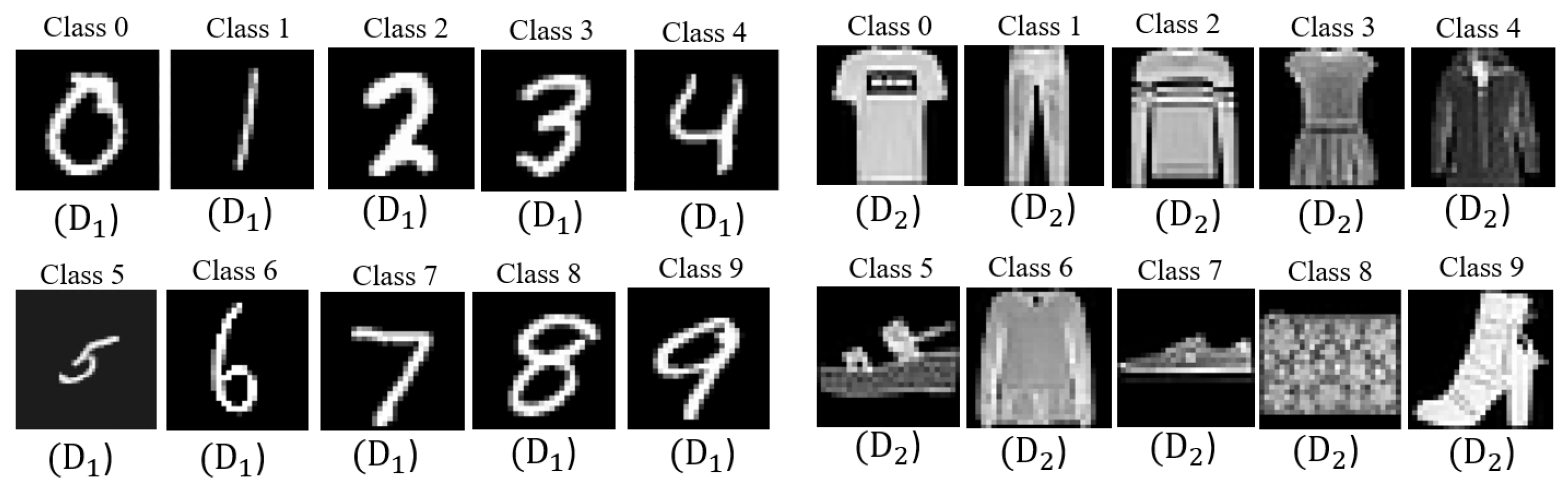
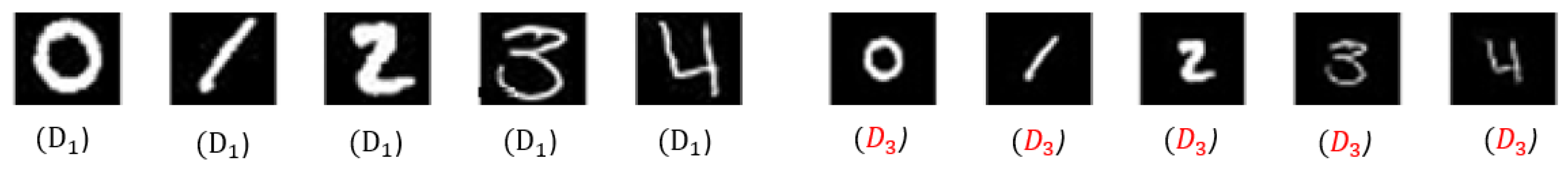
5.1. Data Sets Used for Experimental Investigations

Two standard data sets were used to support the experimental analysis for IID data, denoted by D 1 and D 2 . D 1 is the Modified National Institute of Standards and Technology (MNIST)) set, which was developed for handwriting digit recognition, and D 2 is the Fashion MNIST set, developed for clothes recognition. Both data sets contain 28 × 28 binary images annotated for 10 different classes (Figure 2). For D 2 , the classes were defined as follows: 0 = T-shirt or top, 1 = trousers, 2 = pullover, 3 = dress, 4 = coat, 5 = sandal, 6 = shirt, 7 = sneaker, 8 = bag, and 9 = ankle boot. The experiments were carried out with 42,000 samples from D 1 and 70,000 samples from D 2 .
To configure non-IID data scenarios, another data set was used which also had 42,000 binary images of a size 28 × 28 like D 1 . D 3 was generated from D 1 by reducing the size of the digit in each sample. Therefore, the number of black pixels was larger for the images from D 3 than from D 1 , as indicated in Figure 3. The same aspect is illustrated by the histogram of pixel intensities exemplified in Figure 4 for the samples belonging to class 8. With training samples from D 1 D 3 , the clients could simply be exposed to non-IID data, as exemplified in the next subsection.
In all scenarios, the inputs accepted by the classification models were the intensities of the pixels without any other feature extraction step. The data sets were split into 90% images for training and 10% for validation, while the training samples were distributed to all active clients.

5.2. Federated Learning Settings and Experiment Design

The concept of federated learning requires distributing data among all active clients for local training. As presented in Figure 5, this paper proposes using both IID data (scenarios 1 and 2 applied for D 1 or D 2 ) and non-IID data (scenario 3 applied for D 1 D 3 ). These set-ups are close to real-life scenarios and permit an extensive analysis of FL approaches.
The number of clients always active was set at C = 10, and the analysis was carried out for R = 10 communication rounds, which could illustrate the convergence of the FL process. For several testing scenarios, some less effective clients were simulated to analyze their impact on aggregation. These clients could correspond to intruders or nodes with unsuccessful local training. They were configured only in the first round by disturbing the initial parameters received from the server with additive Gaussian noise of a mean 0 and spread 0.5. During the remaining communication rounds, other disturbances were not considered, as the goal was to analyze how fast the system could recover when dealing with intruders or underperforming local models.
As mentioned before, the local and global models were MLPs. This type of nonlinear model was configured with many neural parameters to offer relevant support for our analysis. The nonlinear neural network thus included three layers with 100, 40, and 10 perceptrons. The first two layers used the ReLU activation function, which facilitates proper learning by reducing the risk of the gradient disappearing. The outputs of the last layer were processed by the softmax function to compute the probabilities associated with all 10 classes. In the case of FedLasso, the outputs of this layer correspond to the term ( z n , i j ) from (12).
The local models were trained using the SGD method, which is widely recommended for MLPs and was also adopted by FedAvg and FedAvgM. All active clients used the same configuration of the training procedure (i.e., they worked with the learning rate η j = 0.01, the same number of epochs E j = 5 for each communication round, and a mini-batch of 32 samples, where j { 1 , , 10 } ). To reduce the impact of the model update obtained at r = 0 (which was likely affected by the negative clients), FedAvgM was configured for β = 0.0001 . Additional results will be provided in the ablation study. Accuracy was used to evaluate the quality of the local models, and during all communication rounds, accuracy was also used to monitor the global model performance. Due to the stochastic nature of learning, each scenario was run 5 independent times, and the resulting mean values were considered for the analysis. The experiments were performed on the proposed methods using Jupyter Notebook, an interactive web-based computing environment, and the Google TensorFlow framework for machine learning.

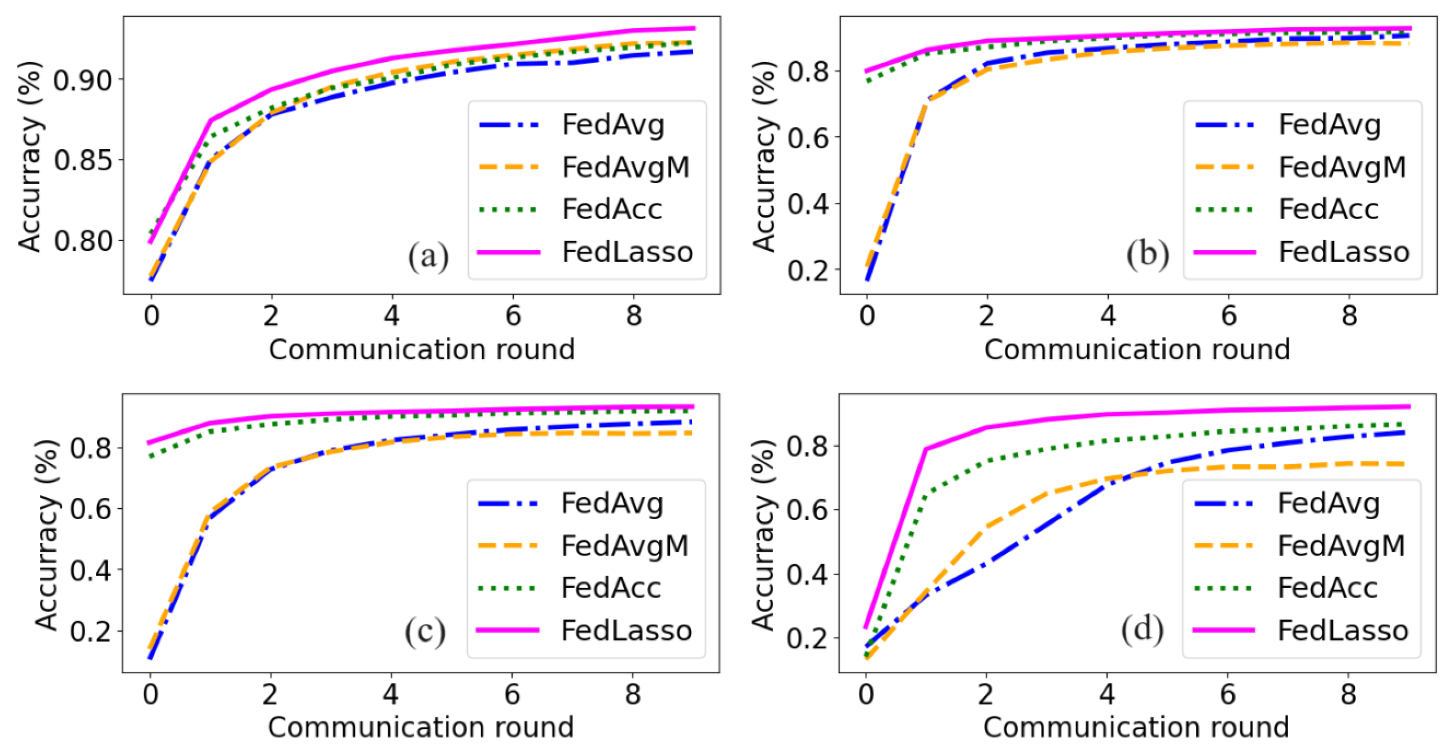
5.3. Results Analysis

The experimental results are presented in this section to compare our proposed methods (FedAcc, FedAccSize, and FedLasso) with established algorithms from the literature (FedAvg and FedAvgM). As previously mentioned, all aggregation methods were examined using the same environment settings for each considered test scenario (the same distribution of data to clients, the same model architecture, etc.).
The results obtained for scenario 1 are illustrated in Figure 6 for the D 1 data set and in Figure 7 for the D 2 data set. In addition, details from the first two communication rounds are provided in Figure 8. This scenario distributed the same amount of training data to the clients, which means that there was no difference between FedAcc and FedAccSize. Some clients were disturbed at the beginning of the first round of communication. They were considered negative because they could deteriorate the performance of FL. The goal of this scenario was to illustrate the influence of the negative clients on the aggregation step (Figure 6b and Figure 7b, scenario 1.2:2 negative clients; Figure 6c and Figure 7c, scenario 1.3:4 negative clients; Figure 6d and Figure 7d, scenario 1.4:8 negative clients). When no negative clients were simulated, the differences between these methods were marginal, as can be observed in Figure 6a and Figure 7a, scenario 1.1 (0 negative clients). As expected, the advantages of FedAcc and FedLasso became visible when some negative clients were simulated. FedAvg and FedAvgM assigned the same weights to all the clients irrespective of their quality, as all the local training data sets had the same sizes. Having no mechanism to detect the negative clients, these algorithms produced a worse global model in the first communication round, and the damage was propagated to all clients in the subsequent rounds, thus making the recovery process longer, as shown in Figure 6 and Figure 7. The experimental results also showed small variations between the performances of FedAvg and FedAvgM. The differences were larger when numerous negative clients were simulated because the momentum technique of FedAvgM propagated the disturbed global model update from the first communication round through the whole learning process.
On the contrary, FedAcc and FedLasso assigned different degrees of confidence to the clients and had the ability to ignore the deteriorated models, as shown in Figure 8. This translated into a more reliable aggregation. As a result, when the negative clients were not majoritarian, FedAcc and FedLasso offered proper protection and did not disturb the global model produced in the first round. In all cases, they recovered much faster than FedAvg and FedAvgM. The differences between FedAcc and FedLasso became visible for D 1 when eight negative clients were simulated (Figure 6d). In this case, the regularization techniques integrated into FedLasso ensured a more effective aggregation. However, both algorithms showed an improved ability to deal with negative clients, even when these clients were in the majority. Stronger protection could be obtained by increasing the threshold indicated for the intermediary coefficients in Equations (6), (7) and (11), but imposing too strict of restrictions for the models accepted for aggregation was not beneficial for the transfer of knowledge requested in FL. For all the other configurations, the differences between FedAcc and FedLasso were minor (e.g., Figure 7d). Some details about the results obtained in the first two rounds are presented in Figure 8. They show the ability of FedAcc and FedLasso to avoid the use of less effective local models and assign larger weights to the most accurate local models. However, due to model nonlinearity, all algorithms had the risk of producing a global model much worse than the local ones. The effect was more visible in the first round when large local updates were obtained.
Scenario 2 shows the case where the IID data were unequally distributed to clients, and half of the clients were negative (Figure 9). This scenario can illustrate the difference between FedAcc and FedAccSize, which in this case computed distinct weights (Figure 10). Unlike FedAcc, FedAccSize also takes into account the size of the local training data set to favor the clients engaged in a difficult but useful learning task. However, Figure 9 shows that there were no significant differences between FedAcc and FedAccSize. This result indicates that accuracy is the most influential factor for FedAccSize and suggests that proper exploitation of model quality could be the key to reliable aggregation. As in the previous scenario, FedAvg and FedAvgM were vulnerable to negative clients, which translated into an important degradation of the global model in the first communication round. As a consequence, the recovery process was much slower for these two methods. This aspect is also exemplified in Figure 10, which shows that in the first communication round, FedAcc, FedAccSize, and FedLasso assigned null weights to all negative clients, thus making it possible to perform the aggregation without being affected by these disturbances. This exemplification also shows that FedAcc, FedAccSize, and FedLasso were able to assign large weights to performing clients, which helped aggregate an accurate global model. Compared to FedAcc, FedAccSize offers larger weights for the clients working with larger training data sets ( j = 6 and j = 7 ). For FedLasso, the relevance of the clients results from the Lasso regression, and this implicitly involves decreasing the weights of some clients detected as redundant (e.g., for r = 0 , clients j = 9 vs. j = 7 , or for r = 1 , clients j = 6 vs. j = 7 ).
The last testing scenario (scenario 3) included non-IID data. To ensure that the clients were exposed to different distributions of data, some clients worked only with samples from D 1 , some clients used only samples from D 3 , and the rest had samples from D 1 D 3 . Half of the clients were simulated as negative. All the local training data sets had the same size to highlight the influence of data distribution on the federated learning process. According to this setting, FedAcc and FedAccSize are similar. The experiments show that D 1 was easier to learn, and models devoted only to this data set achieved better performance from early communication rounds. The explanation is related to the increased redundancy of features related to D 3 , caused by the fact that the samples included many irrelevant black pixels (Figure 4). As a consequence, for FedAcc and FedLasso, there was the risk of treating the models configured with respect to D 3 or D 1 D 3 as less adapted. If the influence of these models was decreased during the aggregation stage, then the global model could not integrate enough data, and its generalization capacity was affected. To highlight this aspect, the validation data set was formed with samples from D 1 (Figure 11a) or with samples from D 1 D 3 (Figure 11b). The first case hid the above-mentioned problem because the local models were not verified for any sample from D 3 . The clients using training samples from D 3 or D 1 D 3 provided less accurate models in the first communication rounds, but without having any indication of their enhanced generalization capability, these models were just processed as performing worse. On the other hand, a validation data set from D 1 D 3 could illustrate that the clients working with samples from a single data set ( D 1 or D 3 ) offered worse results for the validation samples from the other data set. The difficulties in learning D 3 affected the accuracy of the global model in the first few rounds, as shown in Figure 11a versus Figure 11b. According to Figure 11, FedLasso is less vulnerable to these issues than FedAcc. It seems that the redundancy analysis implicitly performed by FedLasso increased the impact of appropriate local models (Figure 12), which improved the global performance. As in previous scenarios, aggregation methods based on accuracy ensured faster and more reliable training than FedAvg or FedAvgM.
As shown in Figure 6, Figure 7 and Figure 9 (scenarios with IID data), and Figure 11 (scenarios with non-IID data), the aggregation based on accuracy (FedAccc and FedAccSize) and aggregation based on Lasso regularization (FedLasso) increased the efficiency of training. Compared with FedAvg and FedAvgM, more accurate models were obtained after a smaller number of communication rounds. This effect was more visible when some negative clients were simulated. The explanation stays in the fact that the methods proposed in this paper use a mechanism to detect negative clients and exclude these clients from aggregation, which reduces the additional effort needed for model training, contrary to FedAvg and FedAvgM. In addition, accepted client models are weighted based on their performance, and the differences between FedAccc, FedAccSize, and FedLasso result from how these weights are computed.

5.4. Ablation Study

The ablation study highlights some important aspects related to the design of FedLasso. The experiments were designed to outline the role of the main steps of the algorithm and possible issues that may arise during FedLasso development. To illustrate the role of the accuracy-based protection mechanism, FedLasso-1 was configured without protection by using all active clients in Equation (10) irrespective of their accuracy (i.e., S ˜ r = S r ). Figure 13 shows that the protection mechanism had an important impact on FedLasso (FedLasso vs. FedLasso-1). All algorithms with accuracy-based protection ensured a faster recovery than algorithms that accepted all local models with non-null weights. This protection becomes quite important for FedLasso because less-adapted models can be detected as being different from the others and associated with high absolute value Lasso coefficients.
In addition, FedLasso-2 was configured with protection but for other covariates than those in the case of FedLasso. For FedLasso-2, the optimization problem in Equation (10) was defined using the probabilities predicted by each client for the target class:
x n j = ( z n , q j ) ,
where q { 1 , , Q } specifies the target class of the nth sample and ( z n , q j ) is the output provided by the softmax layer of the client j for the target class q, considering the nth sample. This configuration allows exploiting detailed information from each client, but as mentioned before, it can generate numerical problems for large or imbalanced data sets. As indicated in Figure 13, the differences between FedLasso and FedLasso-2 were minor. This shows that the covariates proposed in Equation (13) are relevant, even though they have a much smaller size than the covariates in Equation (14). Hence, Lasso regression could be used with the proposed dimensionality reduction.
The last part of the ablation study illustrates the performances of FedLasso working with different values of α using scenario 1.4, which involved majoritarian intruded clients in the first communication round. The values of α were kept small to reduce the influence of the first global model update to the subsequent communication rounds. This configuration was taken into account because this first update was likely to be affected by negative clients who were in the majority. In this context, the variation in α had a reduced impact, as shown in Figure 14. The configuration highlighted in bold, which offered the best results, was adopted for all the other previously presented tests.

6. Conclusions

This paper discusses FL methods that can offer reliable aggregation based on evaluation of the quality of local models. Aggregation was performed at the parameter level without modifying the structure of the resulting global model. Our comparative analysis included two algorithms—FedAcc and FedAccSize—that use the accuracy of the local models to exclude the worse-performing clients from the aggregation and establish weights for the accepted ones. As an extension, FedLasso considers Lasso regression with respect to the outputs of the local models to compute refined weights. In the case of classification problems, Lasso regression is proposed for covariates of a reduced dimension to avoid the numerical problems that can arise for imbalanced and large data sets.
The experimental investigations performed with IID and non-IID data validated that the proposed aggregation techniques were able to provide a more robust and faster improvement of the global model in comparison with two well-known algorithms, FedAvg and FedAvgM. The results highlight the importance of assessing the quality of local models. A key component is the protection mechanism, which permits rejecting potential intruders and worse-performing clients. The comparison between FedAcc and FedAccSize showed that the promotion of clients working with larger data sets is advisable, but the mechanisms exploiting the quality of the models could be more influential. FedLasso integrates an implicit refined analysis of data redundancy, but this can also favor the aggregation of dissimilar less-adapted local models. In this context, the protection mechanism becomes essential for excluding unnecessary models.
The experiments validate that the proposed algorithms (FedAcc, FedAccSize, and FedLasso) are suitable for any practical applications that use sensitive user information to provide safer model fusion and faster training. This analysis highlights the importance of local model performance evaluation for the diagnosis of potential issues related to local designs or cyber-attacks and shows that aggregation can be appropriately performed without isolating the anomalies. Future work will extend the analysis to other testing scenarios and will investigate new aggregation mechanisms that exploit the quality of local models.

Author Contributions

Conceptualization, I.B., L.F. and C.P.; methodology, I.B., L.F. and C.P.; software, I.B. and L.F.; validation, I.B., L.F., C.P. and C.-F.C.; formal analysis, I.B., L.F. and C.P.; investigation, I.B. and L.F.; resources, I.B. and L.F.; data curation, I.B. and L.F.; writing—original draft preparation, I.B.; writing—review and editing, I.B., L.F., C.P. and C.-F.C.; visualization, I.B., L.F. and C.P.; supervision, L.F., C.P. and C.-F.C.; project administration, C.-F.C.; funding acquisition, C.-F.C. All authors have read and agreed to the published version of the manuscript.

Funding

Part of this research was supported by the project “Collaborative environment for developing OpenStack-based cloud architectures with applications in RTI” SMIS 124998 from The European Regional Development Fund through the Competitiveness Operational Program 2014–2020, priority axis 1: Research, technological development and innovation (RTI)—the POC/398/1/1 program.

Institutional Review Board Statement

Not applicable.

Informed Consent Statement

Not applicable.

Data Availability Statement

Data are contained within the article.

Conflicts of Interest

The authors declare no conflict of interest. The funders had no role in the design of the study; in the collection, analyses, or interpretation of data; in the writing of the manuscript; or in the decision to publish the results.

References

  1. McMahan, B.; Moore, E.; Ramage, D.; Hampson, S.; Arcas, B.A. Communication-efficient learning of deep networks from decentralized data. In Proceedings of the Artificial Intelligence and Statistics, PMLR, Fort Lauderdale, FL, USA, 20–22 April 2017; pp. 1273–1282. [Google Scholar]
  2. Konečný, J.; McMahan, H.B.; Yu, F.X.; Richtarik, P.; Suresh, A.T.; Bacon, D. Federated Learning: Strategies for Improving Communication Efficiency. In Proceedings of the NIPS Workshop on Private Multi-Party Machine Learning, Barcelona, Spain, 9 December 2016. [Google Scholar]
  3. Wen, J.; Zhang, Z.; Lan, Y.; Cui, Z.; Cai, J.; Zhang, W. A survey on federated learning: Challenges and applications. Int. J. Mach. Learn. Cybern. 2023, 14, 513–535. [Google Scholar] [PubMed]
  4. Chen, Y.; Qin, X.; Wang, J.; Yu, C.; Gao, W. Fedhealth: A federated transfer learning framework for wearable healthcare. IEEE Intell. Syst. 2020, 35, 83–93. [Google Scholar] [CrossRef]
  5. Rieke, N.; Hancox, J.; Li, W.; Milletari, F.; Roth, H.R.; Albarqouni, S.; Bakas, S.; Galtier, M.N.; Landman, B.A.; Maier-Hein, K.; et al. The future of digital health with federated learning. NPJ Digit. Med. 2020, 3, 119. [Google Scholar] [PubMed]
  6. Yang, T.; Andrew, G.; Eichner, H.; Sun, H.; Li, W.; Kong, N.; Ramage, D.; Beaufays, F. Applied federated learning: Improving google keyboard query suggestions. arXiv 2018, arXiv:1812.02903. [Google Scholar]
  7. Li, Y.; Tao, X.; Zhang, X.; Liu, J.; Xu, J. Privacy-preserved federated learning for autonomous driving. IEEE Trans. Intell. Transp. Syst. 2021, 23, 8423–8434. [Google Scholar] [CrossRef]
  8. Wasilewska, M.; Bogucka, H.; Poor, H.V. Secure Federated Learning for Cognitive Radio Sensing. IEEE Commun. Mag. 2023, 61, 68–73. [Google Scholar]
  9. Barbieri, L.; Savazzi, S.; Brambilla, M.; Nicoli, M. Decentralized federated learning for extended sensing in 6G connected vehicles. Veh. Commun. 2022, 33, 100396. [Google Scholar] [CrossRef]
  10. Yang, Q.; Liu, Y.; Chen, T.; Tong, Y. Federated machine learning: Concept and applications. ACM Trans. Intell. Syst. Technol. (TIST) 2019, 10, 1–19. [Google Scholar]
  11. Feng, C.; Liu, B.; Yu, K.; Goudos, S.K.; Wan, S. Blockchain-empowered decentralized horizontal federated learning for 5G-enabled UAVs. IEEE Trans. Ind. Inform. 2021, 18, 3582–3592. [Google Scholar] [CrossRef]
  12. Wei, K.; Li, J.; Ma, C.; Ding, M.; Wei, S.; Wu, F.; Chen, G.; Ranbaduge, T. Vertical Federated Learning: Challenges, Methodologies and Experiments. arXiv 2022, arXiv:2202.04309. [Google Scholar]
  13. Li, L.; Fan, Y.; Tse, M.; Lin, K.Y. A review of applications in federated learning. Comput. Ind. Eng. 2020, 149, 106854. [Google Scholar] [CrossRef]
  14. Yuan, L.; Sun, L.; Yu, P.S.; Wang, Z. Decentralized Federated Learning: A Survey and Perspective. arXiv 2023, arXiv:2306.01603. [Google Scholar]
  15. Li, T.; Sahu, A.K.; Zaheer, M.; Sanjabi, M.; Talwalkar, A.; Smith, V. Federated optimization in heterogeneous networks. Proc. Mach. Learn. Syst. 2020, 2, 429–450. [Google Scholar]
  16. Zhou, Z.; Sun, F.; Chen, X.; Zhang, D.; Han, T.; Lan, P. A Decentralized Federated Learning Based on Node Selection and Knowledge Distillation. Mathematics 2023, 11, 3162. [Google Scholar] [CrossRef]
  17. Rodríguez-Barroso, N.; Jiménez-López, D.; Luzón, M.V.; Herrera, F.; Martínez-Cámara, E. Survey on federated learning threats: Concepts, taxonomy on attacks and defences, experimental study and challenges. Inf. Fusion 2023, 90, 148–173. [Google Scholar] [CrossRef]
  18. Zhang, C.; Xie, Y.; Bai, H.; Yu, B.; Li, W.; Gao, Y. A survey on federated learning. Knowl.-Based Syst. 2021, 216, 106775. [Google Scholar] [CrossRef]
  19. Mu, X.; Shen, Y.; Cheng, K.; Geng, X.; Fu, J.; Zhang, T.; Zhang, Z. Fedproc: Prototypical contrastive federated learning on non-iid data. Future Gener. Comput. Syst. 2023, 143, 93–104. [Google Scholar] [CrossRef]
  20. Park, J.; Yoon, D.; Yeo, S.; Oh, S. AMBLE: Adjusting mini-batch and local epoch for federated learning with heterogeneous devices. J. Parallel Distrib. Comput. 2022, 170, 13–23. [Google Scholar] [CrossRef]
  21. Zhu, C.; Zhang, J.; Sun, X.; Chen, B.; Meng, W. ADFL: Defending Backdoor Attacks in Federated Learning via Adversarial Distillation. Comput. Secur. 2023, 132, 103366. [Google Scholar] [CrossRef]
  22. Li, A.; Sun, J.; Zeng, X.; Zhang, M.; Li, H.; Chen, Y. Fedmask: Joint computation and communication-efficient personalized federated learning via heterogeneous masking. In Proceedings of the 19th ACM Conference on Embedded Networked Sensor Systems, Coimbra, Portugal, 15–17 November 2021; pp. 42–55. [Google Scholar]
  23. Wu, J.; Wang, Y.; Shen, Z.; Liu, L. Adaptive client and communication optimizations in Federated Learning. Inf. Syst. 2023, 116, 102226. [Google Scholar] [CrossRef]
  24. Ma, C.; Li, J.; Ding, M.; Yang, H.H.; Shu, F.; Quek, T.Q.; Poor, H.V. On safeguarding privacy and security in the framework of federated learning. IEEE Netw. 2020, 34, 242–248. [Google Scholar] [CrossRef]
  25. Bejenar, I.; Ferariu, L.; Pascal, C.; Caruntu, C.F. FedAcc and FedAccSize: Aggregation Methods for Federated Learning Applications. In Proceedings of the 2023 31st Mediterranean Conference on Control and Automation (MED), IEEE, Limassol, Cyprus, 26–29 June 2023; pp. 593–598. [Google Scholar]
  26. Hsu, H.; Qi, H.; Brown, M. Measuring the Effects of Non-Identical Data Distribution for Federated Visual Classification. arXiv 2019, arXiv:1909.06335. [Google Scholar]
  27. Guo, J.; Liu, Z.; Tian, S.; Huang, F.; Jiaxing Li, X.L.; Igorevich, K.K.; Ma, J. TFL-DT: A Trust Evaluation Scheme for Federated Learning in Digital Twin for Mobile Networks. IEEE J. Sel. Areas Commun. 2023, 41, 3548–3560. [Google Scholar] [CrossRef]
  28. Pasquier, T.F.J.M.; Singh, D.E.J.; Bacon, J. CamFlow: Managed Data-sharing for Cloud Services. IEEE Trans. Cloud Comput. 2023, 5, 472–484. [Google Scholar] [CrossRef]
  29. Stergiou, C.L.; Psannis, K.E.; Gupta, B.B. InFeMo: Flexible Big Data management through a federated Cloud system. ACM Trans. Internet Technol. 2021, 22, 1–22. [Google Scholar] [CrossRef]
  30. Wang, H.; Yurochkin, M.; Sun, Y.; Papailiopoulos, D.; Khazaeni, Y. Federated learning with matched averaging. arXiv 2020, arXiv:2002.06440. [Google Scholar]
  31. Palihawadana, C.; Wiratunga, N.; Wijekoon, A.; Kalutarage, H. FedSim: Similarity guided model aggregation for Federated Learning. Neurocomputing 2022, 483, 432–445. [Google Scholar] [CrossRef]
  32. Bagdasaryan, E.; Veit, A.; Hua, Y.; Estrin, D.; Shmatikov, V. How to backdoor federated learning. In Proceedings of the International Conference on Artificial Intelligence and Statistics, PMLR, Online, 26–28 August 2020; pp. 2938–2948. [Google Scholar]
  33. Rodríguez-Barroso, N.; Martínez-Cámara, E.; Luzón, M.V.; Herrera, F. Dynamic defense against byzantine poisoning attacks in federated learning. Future Gener. Comput. Syst. 2022, 133, 1–9. [Google Scholar] [CrossRef]
  34. Yurochkin, M.; Agarwal, M.; Ghosh, S.; Greenewald, K.; Hoang, N.; Khazaeni, Y. Bayesian nonparametric federated learning of neural networks. In Proceedings of the International Conference on Machine Learning, PMLR, Long Beach, CA, USA, 9–15 June 2019; pp. 7252–7261. [Google Scholar]
  35. Chen, H.Y.; Chao, W.L. Fedbe: Making bayesian model ensemble applicable to federated learning. arXiv 2020, arXiv:2009.01974. [Google Scholar]
  36. Czajkowski, M.; Jurczuk, K.; Kretowski, M. Steering the interpretability of decision trees using lasso regression-an evolutionary perspective. Inf. Sci. 2023, 638, 118944. [Google Scholar] [CrossRef]
  37. Fan, Y.; Tao, B.; Zheng, Y.; Jang, S.S. A data-driven soft sensor based on multilayer perceptron neural network with a double LASSO approach. IEEE Trans. Instrum. Meas. 2019, 69, 3972–3979. [Google Scholar] [CrossRef]
  38. Coelho, F.; Costa, M.; Verleysen, M.; Braga, A.P. LASSO multi-objective learning algorithm for feature selection. Soft Comput. 2020, 24, 13209–13217. [Google Scholar] [CrossRef]
  39. Kashima, T.; Kishida, I.; Amma, A.; Nakayama, H. Server Aggregation as Linear Regression: Reformulation for Federated Learning. 2022. Available online: https://openreview.net/pdf?id=kV0cA81Vau (accessed on 30 August 2023).
Figure 1. A flow chart of the federated learning process.
Mathematics 11 04610 g001
Figure 2. Examples of samples belonging to all 10 classes, with left pictures from D 1 (MNIST) and right pictures from D 2 (Fashion MNIST).
Mathematics 11 04610 g002
Figure 3. Examples of samples used for the non-IID data scenario: (left) from D 1 and (right) from D 3 .
Mathematics 11 04610 g003
Figure 4. The histogram of pixel intensities for the samples belonging to class 8 that were used in the non-IID data scenarios, with white bars for D 1 and gray bars for D 3 . The intensities 0 and 255 correspond to black and white pixels, respectively.
Mathematics 11 04610 g004
Figure 5. The distribution of local training data sets for the testing scenarios. The percentage of samples used for each client is marked in regular black text for D 1 or D 2 and in italic red text for D 3 . The intruders are highlighted in gray.
Mathematics 11 04610 g005
Figure 6. Experimental results for scenario 1 using the D 1 data set: (a) scenario 1.1, 0 negative clients; (b) scenario 1.2, 2 negative clients; (c) scenario 1.3, 4 negative clients; and (d) scenario 1.4, 8 negative clients.
Mathematics 11 04610 g006
Figure 7. Experimental results: scenario 1 using the D 2 data set: (a) scenario 1.1, 0 negative clients; (b) scenario 1.2, 2 negative clients; (c) scenario 1.3, 4 negative clients; and (d) scenario 1.4, 8 negative clients.
Mathematics 11 04610 g007
Figure 8. Details about the first two communication rounds for testing scenario 1.4. For each client, the training samples were from D 1 . The negative clients have been highlighted in gray.
Mathematics 11 04610 g008
Figure 9. Experimental results for scenario 2 using 5 negative clients and samples from the (a) D 1 data set and (b) D 2 data set.
Mathematics 11 04610 g009
Figure 10. Details about the first two communication rounds for testing scenario 2. For each client, the training data were from D 1 . The negative clients are highlighted in gray.
Mathematics 11 04610 g010
Figure 11. Experimental results for scenario 3 using 5 negative clients and training samples from D 1 or D 3 : (a) accuracy computed using only validation samples from D 1 and (b) accuracy computed using validation samples from D 1 D 3 data.
Mathematics 11 04610 g011
Figure 12. Details about the first two communication rounds for testing scenario 3. For each client, the training samples were from D 1 or D 3 . The accuracy was computed for samples collected from D 1 D 3 . The negative clients are highlighted in gray.
Mathematics 11 04610 g012
Figure 13. Experimental results for scenario 3 using different configurations of FedLasso. The table contains the average accuracy obtained by 5 independent trials at each communication round using validation samples from D 1 D 3 .
Mathematics 11 04610 g013
Figure 14. Experimental results for FedLasso obtained with different values for α using scenario 1.4. The table contains the average accuracy at each communication round, resulting in 5 independent trials.
Mathematics 11 04610 g014
Table 1. Parameters used in the description of the FL aggregation algorithms.
ParameterDescription
| · | the size of a data set
Rthe number of communication rounds
Cthe total number of clients connected to the server
rindex for iterating the communication rounds
jindex for iterating the clients
S r the subset of active clients during the rth communication round ( S r { 1 , 2 , , C } )
D j the training data set used by the jth client
N r the total number of samples used by all active clients for training during the rth communication round ( N r = j S r | D r j | )
E j the total number of epochs used by the jth client
kindex for iterating the training epochs
η j the learning rate used by the jth client
Jthe loss function adopted for training
ϕ 0 the initial parameters of the global model
ϕ r 1 , ϕ r the parameters of the global model at the beginning and end of the rth communication round, respectively
w r j the weight assigned to the jth client during the rth communication round
β the momentum constant used by the server in the FedAvgM method
L 0 , L 1 , , L M the coefficients used in Lasso regression
ψ r j the intermediary coefficient computed before w r j for client j at the rth communication round
A c c r j the accuracy of the client j at the end of the rth communication round
A c c ¯ r the average accuracy of active clients at the end of the rth communication round
Disclaimer/Publisher’s Note: The statements, opinions and data contained in all publications are solely those of the individual author(s) and contributor(s) and not of MDPI and/or the editor(s). MDPI and/or the editor(s) disclaim responsibility for any injury to people or property resulting from any ideas, methods, instructions or products referred to in the content.

