Optimal Bandwidth Selection Methods with Application to Wind Speed Distribution

Abstract

Accurate estimation of the unknown probability density functions of critical variables, such as wind speed—which plays a pivotal role in harnessing clean energy—is essential for various scientific and practical applications. This research conducts a comprehensive comparative analysis of seven distinct bandwidth calculation techniques across various normal distributions, using simulation as the evaluation method in the context of Kernel Density Estimation (KDE). This analysis includes the calculation of the optimal bandwidth and assessment of the performance of these methods with respect to Mean Squared Error (MSE), bias, and the optimal bandwidth value. The findings reveal that among the various bandwidth methods evaluated, the Bandwidth bandwidth-based Cross-Validation (BCV), especially for small sample sizes, consistently provides the closest result to the optimal bandwidth across most of the applied normal distributions. These results provide valuable insights into the selection of optimal bandwidths for accurate and reliable density estimation in the context of normal distributions. Another key aspect of this work is the extension of these methods to wind speed data in a specific region. Monthly wind speed kernel density estimates obtained using all seven bandwidth selection techniques show that Smoothed Cross-Validation (SCV) is suited for this type of real-world data.

1. Introduction

Driven by technological advancements and environmental repercussions from fossil fuel consumption, wind energy has become an increasingly popular source of renewable energy, especially since the latter half of the 20th century. This evolution has led to an intensification of research on wind speed, which is a source of energy production [1,2,3]. With wind speed playing a pivotal role in energy production, accurately estimating its Probability Density Function (PDF) has become imperative. While the Weibull distribution was historically the method of choice for this purpose, “kernel density” estimators have recently emerged as a preferred alternative due to their minimal assumptions [4,5].

The Probability Density Function (PDF), which allows for the description of all the properties of the variable, forms the basis of statistical analysis. Knowing the probability density function of a random variable allows one to obtain the location $\left(\mu \right)$ and scale parameter $\left({\sigma }^2\right)$ of that random variable and to answer all probability questions about that random variable. For this reason, PDFs of variables are needed in many analyses. Parametric and non-parametric methods are used in probability density estimations. While parametric methods predicate on the assumption that a designated PDF is the definitive one, non-parametric methods offer a refined estimation, enabling the random variable to represent itself more authentically [6,7].

The performance of kernel density estimators, however, is highly dependent on the choice of “bandwidth”. For example, when small bandwidths are selected, the tails of the scatter will have unrealistic roughness, while when large bandwidths are selected, the tails of the scatter will be excessively flattened, thus losing important features of the scatter. Although it is not possible to determine a single best selection method in bandwidth selection, the population structure in which the data to be estimated for density is observed has great importance [8].

Numerous researchers such as [6,9,10,11,12] have delved into bandwidth selection methods in kernel density estimation. To provide a comprehensive overview, this discussion also encompasses recent publications on the topic. Cao et al. [13] reviewed bandwidth selection in density estimation, noting the limitations of Least Squares Cross-validation (LSCV). They advocate for Direct Plug-In (DPI) and smoothed bootstrap-based methods as superior alternatives for KDE applications on real data. The authors of [14,15] emphasized the significance of exploratory data analysis and graphical representation in kernel density estimates. Their main challenge is selecting the appropriate bandwidth for accurate density depiction in KDE. Simulations revealed that the Sheather-Jones plug-in is optimal, especially for sample sizes between 250 and 2000. For smaller datasets, Silverman’s Rule of Thumb (SRT) is advised [14]. A more in-depth analysis by the same authors showed a similar preference for the Sheather-Jones plug-in but with a tilt towards BCV or SRT for smaller samples [15]. Practitioners applying KDE to their datasets can significantly benefit from these insights. Another recent study spotlighted the effectiveness of adaptive kernel density estimators with long-tail or multi-mode densities. The generalized LSCV has shown superiority over traditional methods in simulations [16]. For optimal results in real-world applications, an adaptive approach with this form of cross-validation is recommended. Various bandwidth comparisons by authors [13,14,15,16] involved metrics like Mean Error Squared (MSE), Integrated Mean Squared Error (MISE), and bias.

In the referenced study [17], the authors explored the influence of bandwidth selection on equated scores in kernel equating. They highlighted the importance of bandwidth choice, as it delineates kernel equating from conventional equating methods. The research scrutinized four established bandwidth methods: penalty, double smoothing, likelihood cross-validation, and SRT. These methods, traditionally compared only to the penalty method, were assessed alongside two other techniques from density estimation literature: leave-one-out cross-validation and penalized leave-one-out cross-validation. Through simulation studies on varying test length, test-taker numbers, and score distributions, and an empirical evaluation using college admissions data, the authors aimed to discern the most effective bandwidth selection approach for kernel equating.

According to [18], various bandwidth selection methods were evaluated, and it was found that the BCV method demonstrated consistent precision for specific normal mixture densities. Recent research emphasized novel methods for selecting optimal bandwidths in KDE without relying on a normal (Gaussian) distribution. New bandwidth rules based on other distributions such as Logistic, Laplace, Student’s t, and Asymmetric Laplace have been proposed. Additionally, a pseudo-rule-of-thumb bandwidth derived from data skewness and kurtosis characteristics offers a straightforward implementation approach [19].

As the emphasis on harnessing wind energy intensifies, there has been a surge in studies aiming for more precise predictions of wind speed distribution in recent years.

Wind speeds on both a monthly and yearly basis are statistically represented using the Weibull distribution. The assessment of the model’s accuracy is conducted through the evaluation of the root mean square error [20]. A mixture kernel density model for wind speed distribution estimation is being proposed by [21]. Another study presents a KDE method, which is a nonparametric way to estimate the PDF of wind speed [22]. Monthly wind speed data from three specific weather stations were analyzed by Citakoğlu and Aydemir [23] using the Gray estimation method, covering the period from 2000 to 2017. Four bandwidth selectors, namely Normal Scale (NS, DPI, BCV, and LSCV, are employed in wind speed modeling for the KDE model, and they showed that KDE performs better than parametric methods [24]. The authors of [25] introduced a framework for short-term wind speed probability density forecasting, utilizing Quantile Regression (QR) and KDE. The authors of [26] presented and analyzed a flexible distribution referred to as the Alpha logarithmic transformed Log-normal for wind speed data. They conducted an analysis of real data using this newly proposed distribution. Additionally, they introduced a new model known as the Normal-Weibull-Weibull model, which is identifiable, and its cumulative distribution function is expressed as a composition of two foundational functions. In another research study [27], an enhanced KDE method, termed ensemble unbiased cross-validation-based KDE, was introduced to address the instability concerns inherent to traditional unbiased cross-validation. Through the utilization of multiple data-block unbiased cross-validations instead of a singular approach, a more stable bandwidth estimation was achieved. Experiments on ten probability distributions validated its superior stability and performance, which was further evidenced in an application using the United Kingdom climate data for kernel regression.

Daily wind speed data at two different heights (10 m and 50 m) in four regions of Iraq (Al-Rutba, Sinjar, Al-Qa’im, and Al-Bayji) have been analyzed using the Weibull distribution function [28]. One of the recent studies, conducted by [29], has explored the intricacies of wind speed distribution in various regions, emphasizing the temporal variability of these distributions. Their findings reveal the significance of kernel function shape and peak value in the accuracy of KDE. Specifically, their introduction of new kernel functions and a unique point-to-point comparison method showcase the evolving methods and techniques in this domain.

The authors [30] presented a novel kernel density estimator model employing an unbiased cross-validation method for bandwidth selection was introduced. This model was designed to estimate the probability densities of both wind speed and solar irradiance. Its performance was compared against traditional parametric models and another nonparametric KDE approach using several assessment metrics: the coefficient of determination, mean absolute error, root mean squared error, and the Kolmogorov–Smirnov test. Significant improvements in accuracy and fit were demonstrated by the proposed model when benchmarked against popular parametric distributions for wind speed and solar irradiance.

In a study of wind energy in northern China’s desert steppe terrains (2018–2020), the Weibull wind speed distribution proved most fitting. Key parameters in the Weibull model, including the scale factor (c) and shape factor (k), varied with height, while surface roughness (z0) fluctuated between 0.12 m to 0.15 m across different periods. These dynamic changes are vital for accurate wind energy estimates in such terrains [31].

In [32], the authors proposed an alternative distribution, referred to as the Normal-Weibull-Weibull model, which exhibits identifiability and offers a decent fit to the wind speed data. This model’s cumulative distribution function can be expressed as a composition of two foundational functions.

The core objective of this study is to compare the performance of several commonly used bandwidth selection methods that impact kernel density estimation across various normal mixture distributions and to extend these bandwidth selection methods to wind speed, which is real-world data:

• Through simulation study comparisons of seven bandwidth selectors, including NS, SRT, DPI, Solve-The-Equation rules (STE), least LSCV, BCV, and SCV are examined. The results show that, among the different bandwidth techniques assessed, the BCV method—particularly for smaller sample sizes—consistently aligns closest with the optimal bandwidth for a majority of the tested normal distributions.
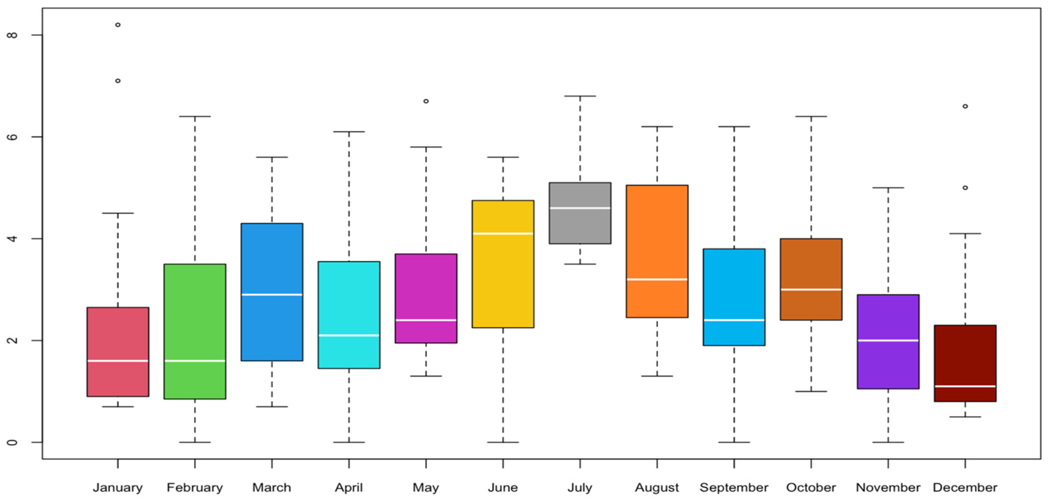
• Wind speed data from Balıkesir, Kepsut region for the year 2022 were employed, with monthly kernel density estimations being conducted using the seven bandwidth selection methods. It was found that the SCV method is convenient for estimating bandwidth for kernel density estimation in most cases with these real-world data.

Collectively, the contribution of the study lies in its multifaceted approach, blending detailed data analysis with theoretical rigor, providing both a unique application to wind speed data and a broader understanding of bandwidth selection methodologies in the context of kernel density estimation. While many comparisons of bandwidth selection methods have been undertaken, these methods have been specifically applied to wind speed data from the Balıkesir, Kepsut region for the year 2022 in this study. A bridge between general kernel density estimation techniques and their application to wind speed data, vital for renewable energy research, has been established. A detailed temporal view of wind speed variations has been provided through a focus on monthly kernel density estimations, offering unique insights not found in broader time-scale analyses. Even though bandwidth selection methods have been compared before, the use of simulation studies that consider different parameter choices and sample sizes ranging from small to large adds another layer of validation, ensuring that findings are not only theoretically robust but also practically applicable. A comprehensive perspective on bandwidth selection, encompassing a wide range of past research, has been offered. As such, this study can be recognized as a consolidated source of information on the topic, serving those seeking an integrated understanding. It has been observed that the SCV method is particularly suitable for estimating bandwidth in the specific dataset used. This nuanced insight may not have been revealed in other contexts or datasets.

The rest of the article has been prepared as follows: the second section elaborates on kernel density estimation and evaluation criteria, the third details the bandwidth methods, the fourth presents a simulation study supported by R (version 4.2.2) for bandwidth performance comparisons, the fifth applies the bandwidths to a real dataset, the sixth provides results, and the seventh section draws conclusions of the findings.

2. Kernel Density Estimation

$x_1,x_2,\dots ,x_n$ are independent and identically distributed samples from an unknown density $f$. The goal is to estimate the shape of this unknown function $f$ the kernel density. Kernel density estimator of the unknown PDF is as follows:

$${\tilde{f}}_{n,h}\left(x\right)=\frac{1}{n·h}{\sum }_{i=1}^{n}K\left(\frac{x-X_i}{h}\right)=\frac{1}{n·h}{\sum }_{i=1}^{n}K\left(t\right)=\frac{1}{n}{\sum }_{i=1}^n{K}_h\left(x-X_i\right).$$

(1)

where $h$ is a smoothing parameter called the bandwidth with positive value ($h>0)$ and K(t) is a kernel function that satisfies ${\int }_{-\infty }^{+\infty }K(t)dt=1$, $\int tK(t)dt=0$, $\int u^{2}K(u)du={\mu }_2(K)>0$. K(t) is generally non-negative, unimodal, and symmetrical about zero. This ensures that ${\tilde{f}}_{n,h}\left(x\right)$ is a PDF [33]. The kernel estimates obviously depend on the bandwidth $h$, which controls the degree of smoothing applied to the data.

MSE is a common criterion used to measure the accuracy or goodness of fit of a statistical estimation or prediction, including KDE. In the context of KDE, MSE is used to evaluate how well the estimated PDF matches the true underlying distribution. The MSE of KDE can be written as follows:

$$MSE\left({\tilde{f}}_{n,h}\left(x\right)\right)=Var\left({\tilde{f}}_{n,h}\left(x\right)\right)+{\left(E\left({\tilde{f}}_{n,h}\left(x\right)\right)-f\left(x\right)\right)}^2.$$

(2)

Here, the expected value of the smoothed density function estimator (${\tilde{f}}_{n,h}\left(x\right)$) and bias are as follows:

$$E{(\tilde{f}}_{n,h}\left(x\right))=f\left(x\right)+\frac{1}{2}{h}^2{f}^{″}(x)\int z^{2}K(z)dz+o\left(h^2\right)$$

(3)

$$E{(\tilde{f}}_{n,h}\left(x\right))-f\left(x\right)=\frac{1}{2}{h}^2{\mu }_2\left(K\right)f^{″}\left(x\right)+o\left(h^2\right),$$

(4)

where ${\mu }_2\left(K\right)=\int z^{2}K(z)dz$ and the expression for the variance of ${\tilde{f}}_{n,h}\left(x\right)$ is:

$$Var\left({\tilde{f}}_{n,h}\left(x\right)\right)={\left(nh\right)}^{-1}\int {K\left(z\right)}^{2}f\left(x-hz\right)dz-n^{-1}{\left(E\left({\tilde{f}}_{n,h}\left(x\right)\right)\right)}^2,$$

(5)

$${=\left(nh\right)}^{-1}\int {K\left(z\right)}^2\left(f\left(x\right)+o\left(1\right)\right)dz-n^{-1}{\left(f\left(x\right)+o\left(1\right)\right)}^2,$$

(6)

$$={\left(nh\right)}^{-1}\int {K\left(z\right)}^{2}dzf\left(x\right)+o\left({\left(nh\right)}^{-1}\right)$$

(7)

For any integrable square function $g$, it is $R\left(g\right)=\int g{(x)}^2$. This allows the variance to be written as:

$$Var\left({\tilde{f}}_{n,h}\left(x\right)\right)={(nh)}^{-1}{h}^{2}R\left(K\right)f\left(x\right)+o\left({\left(nh\right)}^{-1}\right).$$

(8)

where $R\left(K\right)=\int K{(x)}^{2}dx$, ${\mu }_2\left(K\right)=\int x^{2}K(x)dx$, $R\left(f^{″}\right)=\int f^{″}{(x)}^{2}dx$. For the standard normal kernel and univariate cases, it is $R\left(K\right)={{(2\pi }^{1/2})}^{-1}$, ${\mu }_2\left(K\right)=1$, $R\left(f^{″}\right)={{3(8\pi }^{1/2})}^{-1}$. Thus, MSE is expressed as follows:

$$\mathrm{M}\mathrm{S}\mathrm{E}\left({\tilde{f}}_{n,h}\left(x\right)\right)={(nh)}^{-1}R\left(K\right)f\left(x\right)+\frac{1}{4}{h}^4{\mu }_2{(K)}^2{f}^{″}{(x)}^2+o\left({\left(nh\right)}^{-1}+h^4\right)$$

(9)

However, MISE is preferred over MSE in KDE because it is better suited for assessing the accuracy of PDF estimates across the entire data space. It considers the global behavior of the estimator and incorporates the trade-off between bias and variance, making it a more appropriate criterion for evaluating KDE performance, and it can be written as follows:

$$\mathrm{M}\mathrm{I}\mathrm{S}\mathrm{E}\left({\tilde{f}}_{n,h}\left(·\right)\right)={\int }_{-\infty }^{+\infty }E\left({\left({(\tilde{f}}_{n,h}\left(x\right)-f(x)\right)}^2\right)dx={\int }_{-\infty }^{+\infty }MSE\left({\tilde{f}}_{n,h}\left(x\right)\right)dx$$

(10)

$$={\int }_{-\infty }^{+\infty }Var\left({\tilde{f}}_{n,h}\left(x\right)\right)dx+{\int }_{-\infty }^{+\infty }{Bias}^2\left({\tilde{f}}_{n,h}\left(x\right)\right)dx$$

(11)

$$\mathrm{M}\mathrm{I}\mathrm{S}\mathrm{E}\left({\tilde{f}}_{n,h}\left(·\right)\right)=AMISE{(\tilde{f}}_{n,h}\left(·\right))+o\left({\left(nh\right)}^{-1}+h^4\right)$$

(12)

where $\mathrm{A}\mathrm{M}\mathrm{I}\mathrm{S}\mathrm{E}$ stands for Asymptotic $\mathrm{M}\mathrm{I}\mathrm{S}\mathrm{E}$ and $\mathrm{A}\mathrm{M}\mathrm{I}\mathrm{S}\mathrm{E}$ are expressed as follows [33]:

$$\mathrm{A}\mathrm{M}\mathrm{I}\mathrm{S}\mathrm{E}\left({\tilde{f}}_{n,h}\left(·\right)\right)={(nh)}^{-1}R\left(K\right)+\frac{1}{4}{h}^4{\mu }_2{\left(K\right)}^{2}R(f^{″})$$

(13)

$$\mathrm{A}\mathrm{M}\mathrm{I}\mathrm{S}\mathrm{E}\left({\tilde{f}}_{n,h}\left(·\right)\right)={(nh)}^{-1}R\left(K\right)+\frac{1}{4}{h}^4{\mu }_2{\left(K\right)}^2{\Psi }_4$$

(14)

where ${\Psi }_4={\int }_{-\infty }^{\infty }{f}^{\left(4\right)}(x)f(x)dx$ or more general ${\Psi }_r={\int }_{-\infty }^{+\infty }{f}^{\left(r\right)}(x)f(x)dx=E(f^r\left(X\right))$.

Hence, the optimum bandwidth value that minimizes the $\mathrm{M}\mathrm{I}\mathrm{S}\mathrm{E}$ or $\mathrm{A}\mathrm{M}\mathrm{I}\mathrm{S}\mathrm{E}$ can be found:

$$h_{MISE}\sim h_{AMISE}={\left[\frac{R(K)}{n{\mu }_2{\left(K\right)}^{2}R(f^{″})}\right]}^{1/5}={\left[\frac{R(K)}{n{\mu }_2{\left(K\right)}^2{\Psi }_4}\right]}^{1/5}.$$

(15)

For the standard normal kernel and univariate cases, when $R\left(K\right)$, ${\mu }_2\left(K\right)$, $R\left(f^{″}\right)$ values are substituted in Equation (13)

$$\mathrm{A}\mathrm{M}\mathrm{I}\mathrm{S}\mathrm{E}\left({\tilde{f}}_{n,h}\left(·\right)\right)=\frac{5}{4}{\left({\mu }_2{\left(K\right)}^{2}R{\left(K\right)}^{4}R(f^{″})\right)}^{1/5}{n}^{-4/5}$$

(16)

is obtained. This is the smallest possible $\mathrm{A}\mathrm{M}\mathrm{I}\mathrm{S}\mathrm{E}$ for estimating $f$ using the $K$ kernel. Since Equation (15) depends on the unknown density $f(x)$, $f(x)$ must be estimated first. There are different bandwidth selection methods where $f(x)$ is estimated in various ways.

3. Bandwidth Selection Methods

The performance of the kernel density estimators of a PDF of a random variable largely depends on the choice of bandwidth, also known as the smoothing parameter. In other words, it is a value that controls the amount of bandwidth smoothing. Bandwidth can be chosen subjectively in many cases. The subjective selection is made by comparing the graphs of the PDFs, the estimation generated by applying different bandwidths to the random variable. As a result of different bandwidth trials, the most appropriate bandwidth is decided by looking at the appearance of the PDFs. However, such an approach will not give good estimates while giving repeatable results. It is also a time-consuming and error-prone method of trial and error. Another disadvantage is that there is often no a priori knowledge of the data structure and no clue as to which bandwidth gives the closest estimate of true density. The only situation in which subjective selection is useful is when the researcher believes there is a certain construct about the position of the random variable’s mode. Therefore, automatic selection is often required when determining the bandwidth of kernel estimators [33].

Very large bandwidths are expected to yield extremely flattened density estimates with little ‘randomness’. This causes the PDF to deviate from its true form and to make the predictions biased. Small bandwidths, on the other hand, are expected to yield fluctuating (curvy) density estimates with high randomness. In this case, the bias of the estimation decreases, while the variance increases. These two situations prevent us from seeing the properties of the distribution. For this reason, attention should be paid to the most accurate selection of the bandwidth. Bandwidth selection methods fall into three classes.

The selections in the first class are based on finding the optimum bandwidth, starting from a wide range and narrowing it down with a very simple and easy-to-calculate mathematical formula. They are developed to cover a wide range of situations, but they do not guarantee that the result is close enough to the optimum bandwidth. Such selections provide a reasonable starting point for subjectively chosen bandwidths.

Second-class selections are selection processes that are based on a more precise mathematical basis and require much more computational power to arrive at the actual function underlying the dataset. Each of these selection types aims to make the MISE the smallest, and they achieve this goal asymptotically. Therefore, it is said that the bandwidth selection methods obtained by making the MISE the smallest are consistent [34]. These bandwidth selection methods: least squares cross-validation, sometimes also called unbiased cross-validation, are BCV and flattened cross-validation methods [33].

Third-class selections are methods based on substituting (addition) the estimates of some unknown parameters that appear in the formulas for asymptotically optimal bandwidth. These bandwidth selection methods are called substitution and equation solving [8,35]. These selection methods will be briefly introduced.

3.1. Normal Scale Bandwidth Selection Method

When estimating the PDF $f\left(x\right)$ of the data, the bandwidth that minimizes the MISE asymptotically should be chosen. The NS bandwidth selection method is improved by replacing the unknown PDF with a known distribution function.

Usually, the unknown $f\left(x\right)$ is assumed to come from the normal distribution with mean $\mu$ and variance ${\sigma }^2$. With this assumption, the integral of the square of the second derivative of $f$ found in Equation (15) is as follows:

$$\int {\left(f^{″}\left(x\right)\right)}^{2}dx=\frac{3}{8\sqrt{\pi }{\sigma }^5}\approx 0.212{\sigma }^{-5}$$

(17)

When the normal kernel function is used here, it becomes

$$\int K^2\left(u\right)du=\frac{1}{\sqrt{4\pi }}\mathrm{and}\int u^{2}K\left(u\right)du.$$

(18)

Thus, the optimum bandwidth is obtained as

$$h_{opt}={(4\pi )}^{-1/10}{\left(\frac{3}{8}\right)}^{-1/5}{\pi }^{1/10}\sigma n^{-1/5}=1.059\sigma n^{-1/5}$$

(19)

and this bandwidth is approximately

$$h_{opt}=1.06\sigma n^{-1/5}.$$

(20)

Here, if $\widehat{\sigma }=s$, sample standard deviation is substituted for $\sigma$, and the optimal bandwidth is calculated as [6,33]:

$$h_{opt}=1.06\widehat{\sigma }{n}^{-1/5}$$

(21)

It should be noted that the assumption that $f\left(x\right)$ comes from a normal distribution is contrary to the understanding of non-parametric density estimation. If it were known that the random variable $X$ had a normal distribution, density could have been estimated much more easily and efficiently by simply estimating the sample mean $\mu$ and sample variance ${\sigma }^2$ and putting these estimates into the normal density formula. However, the result obtained under the assumption of normality is a clear and applicable formula for bandwidth selection. If the random variable $X$ is normally distributed, choosing the NS bandwidth gives the optimum bandwidth. The distribution of the random variable $X$ is usually unknown, and in such a case, it gives a near-optimal bandwidth if the distribution of $X$ is not significantly different from the normal distribution [8].

3.2. Silverman’s Rule of Thumb Bandwidth Selection Method

Equation (21) gives a near-optimal bandwidth if the distribution of $X$ is not much different from the normal distribution. Therefore, Equation (21) would be a practical bandwidth that would yield good results for all unimodal and highly symmetrical distributions. A robust estimator was used especially in datasets containing outlier observations. Again, under the assumption of normal distribution, the standard deviation $\widehat{\sigma }$ is estimated from the sample instead of $\sigma$ and the sample interquartile range $R$, with the values of

$$A=\min \left(\widehat{\sigma },\frac{R}{1.34}\right)$$

(22)

and the optimal bandwidth [6,34],

$$h_{opt}=1.79R{n}^{-1/5}\mathrm{or}{h}_{opt}=0.9A{n}^{-1/5}$$

(23)

Since this method, first proposed by B.W. Silverman, is performed by replacing the unknown function with a known distribution, it is called SRT bandwidth selection method [6].

3.3. Direct Plug in Bandwidth Selection Method

The DPI bandwidth selection method proposed by [12] has many desirable features in terms of both theory and practice, especially in terms of fast convergence rate and low sampling variability. DPI bandwidth selection method is also referred to as DPI. These features make the substitution bandwidth selection method a first choice in practical applications. This selection method is based on the AMISE criterion. Equation (24) is based on placing an estimator in place of a single unknown ${\Psi }_4$ value in the bandwidth that minimizes the AMISE when ${\Psi }_4$ is replaced by ${\Psi }_4(g_4)$ kernel estimator in Equation (24) obtained as follows:

$${\widehat{h}}_{DPI}={\left[\frac{\int K{(u)}^{2}du}{n{\mu }_2{\left(K\right)}^2{\Psi }_4(g_4)}\right]}^{1/5}$$

(24)

This estimator cannot be used directly as it depends on the unknown value of $g_4$. The authors of [33] showed that $g_4$ can be calculated using the AMISE optimal bandwidth formula. $g_r$ express in the form:

$$g_{r,AMSE}={\left[\frac{2K^{\left(r\right)}(0)}{-n{\mu }_2(K){\Psi }_{r+2}(g_{r+2})}\right]}^{1/(r+3)}.$$

(25)

where AMSE stands for Asymptotic MSE.

If $f$ is a normal density with variance ${\sigma }^2$ then, for $r$, even,

$${\Psi }_r=\frac{{(-1)}^{r/2}r!}{{\left(2\sigma \right)}^{r+1}(r/2)!{\pi }^{1/2}}.$$

(26)

It is generally recommended that the bandwidth is selected in at least two stages. The substitution bandwidth method, which estimates the bandwidth at all these stages, requires very costly calculations [33].

3.4. Solve-the-Equation Rules Bandwidth Selection Method

In Equation (24), STE bandwidth selection method, which brings a different perspective to the substitution bandwidth selection method, there is an additional requirement for the estimation of ${\Psi }_4$ that the pilot bandwidth h has a function of $\gamma$, i.e.,

$${\widehat{h}}_{DPI}={\left[\frac{\int K{(u)}^{2}du}{n{\mu }_2{\left(K\right)}^2{\Psi }_4(\gamma (h))}\right]}^{1/5}$$

(27)

$\gamma (h)$ formula is as follows [8]:

$$\gamma (h)={\left[\frac{{2K}^{\left(4\right)}(0){\mu }_2(K){\widehat{\Psi }}_4(g_4)}{-{\widehat{\Psi }}_6(g_6)R(K)}\right]}^{1/7}{h}^{5/7}$$

(28)

3.5. Least Squares Cross Validation Bandwidth Selection Method

LSCV bandwidth selection method is one of the most frequently used methods in bandwidth selection. It is a technique based on computer-intensive computations and has no clear formulation. An initial assessment of $h$ value is made by drawing a rough histogram. Accordingly, in the next algorithm operation, the value that makes the MISE function the smallest is selected under the $h$ values in a range. Since ${\tilde{f}}_{n,h,-i}\left(x\right)$ excludes an $X_i$ value when estimating density, it is often referred to as the “one observation out” density estimator. The reason why it is called cross-validation is that it makes inferences about the other part by using one part of the sample. The starting point of this method is Integrated Squared Error (ISE), which is an alternative distance measure between $f\left(x\right)$ and ${\tilde{f}}_{n,h}\left(x\right)$ defined in Equation (29) [10]:

$$\begin{array}{cc}\hfill \mathrm{I}\mathrm{S}\mathrm{E}\left({\tilde{f}}_{n,h}\left(x\right)\right)& =\int {\left({\tilde{f}}_{n,h}\left(x\right)-f\left(x\right)\right)}^{2}dx,\hfill \\ & =\int {{\tilde{f}}_{n,h}\left(x\right)}^{2}dx-2\int f\left(x\right){\tilde{f}}_{n,h}\left(x\right)dx+\int {f(x)}^{2}dx.\hfill \end{array}$$

(29)

The goal is to choose a value of $h$ that will make the ISE as small as possible. However, it does not depend on Equation (29) $h$. Therefore, the expected value of the ISE is taken,

$$\mathrm{M}\mathrm{I}\mathrm{S}\mathrm{E}\left({\tilde{f}}_{n,h}\left(x\right)\right)=E\left(\int {{\tilde{f}}_{n,h}\left(x\right)}^{2}dx\right)-2\left(E\left(\int {\tilde{f}}_{n,h}\left(x\right)f\left(x\right)dx\right)\right)+\int {f(x)}^{2}dx$$

(30)

and in this equation, the term $\int {f(x)}^{2}dx$ does not depend on $h$ and does not affect the choice of $h$ and optimality. Therefore, it can be neglected and

$$\mathrm{M}\mathrm{I}\mathrm{S}\mathrm{E} {\tilde{f}}_{n,h}\left(x\right)-\int {f\left(x\right)}^{2}dx=E\int {{\tilde{f}}_{n,h}\left(x\right)}^{2}dx-2\left(E\left(\int {\tilde{f}}_{n,h}\left(x\right)f\left(x\right)dx\right)\right)$$

(31)

obtained.

The right-hand side of Equation (31) cannot be known since it depends on $f(x)$. However, it can be shown to be an unbiased LSCV estimator for this:

$$\mathrm{L}\mathrm{S}\mathrm{C}\mathrm{V}=\frac{1}{n}{\sum }_{i=1}^n\int {\tilde{f}}_{n,h,-i}\left(x\right){(x)}^{2}dx-2n^{-1}{\sum }_{i=1}^n{\tilde{f}}_{n,h,-i}\left(x\right)(x_i).$$

(32)

Here,

$${\tilde{f}}_{n,h,-i}\left(x\right)={(n-1)}^{-1}{\sum }_{j\ne i}^n{K}_h(x-X_j).$$

(33)

The h value that minimizes the LSCV value is chosen as the bandwidth. The authors of [33,36] proved that the LSCV bandwidth selector is easier to calculate in Equation (34):

$$\mathrm{L}\mathrm{S}\mathrm{C}\mathrm{V}=\int {\tilde{f}}_{n,h}\left(x\right)dx-2n^{-1}{\sum }_{i=1}^n{\tilde{f}}_{n,h,-i}(x_i).$$

(34)

Although the LSCV method is frequently used, the large sample variability is a disadvantage. For this reason, due to high variability, the LSCV method, which results in incomplete smoothing in the density estimation, performs poorly at almost all estimated densities compared to other bandwidth selectors [7,10,37].

3.6. Bias Cross Validation Bandwidth Selection Method

To improve the sample variability of the LSCV bandwidth selection method, the authors of [11] proposed the BCV bandwidth selection method. The difference between this method and LSCV is that it is based on AMISE given in Equations (12) and (13) instead of ISE.

In the BCV bandwidth selection method, the unknown $R(f^{″}$) is replaced by an estimator $R({\tilde{f}}^{″})$. This produces a biased estimate [11]:

$${\mathrm{B}\mathrm{C}\mathrm{V}=(nh)}^{-1}R\left(K\right)+\frac{1}{4}{h}^4{\mu }_2{\left(K\right)}^{2}R({\tilde{f}}^{″}).$$

(35)

It reduces the amount of sample variability that causes many of the problems mentioned in BCV, LSCV, and other bandwidths. Also, its asymptotic variance is considerably lower than that of LSCV. However, this decrease in variance causes an increase in bias [34]. Simulation studies conducted by authors [13,37,38] demonstrated that the performance of BCV is superior to that of LSCV.

3.7. Smoothed Cross Validation Bandwidth Selection Method

The SCV bandwidth selection method is similar to substitution bandwidth selection in that the MISE uses a kernel estimator with g pilot bandwidth to estimate the Integrated Squared Bias (ISB) component. Therefore, the methods have similar theoretical properties. The difference is that SCV is based on the integral of the square of the bias rather than the asymptotic approach. Therefore, it has the feature of being less dependent on the asymptotic approximation. The SCV objective function is obtained by replacing $f(x)$ with a pilot estimator:

$${\tilde{f}}_{n,g}(x)=\frac{1}{n}{\sum }_{i=1}^n{L}_g(x-X_i).$$

(36)

Here, $L_g(x)$’s are kernel functions obtained with $g$’s of different bandwidths. Also, SCV containing the asymptotic integrated variance ${\left(nh\right)}^{-1}R(K)$ is estimated with

$$\mathrm{S}\mathrm{C}\mathrm{V}(h)=\frac{1}{nh}R(K)+\mathrm{I}\mathrm{S}\mathrm{B}(h)$$

(37)

with ISB is estimated:

$$\mathrm{I}\mathrm{S}\mathrm{B}(h)=n^{-2}{\sum }_{i=1}^n{\sum }_{j=1}^n{\left(K_h\ast {\tilde{f}}_{n,g}\left(x\right)-\left({\tilde{f}}_{n,g}(x)\right)\right)}^{2}dx$$

(38)

$h_{SCV}$ is the largest minimum of $\mathrm{S}\mathrm{C}\mathrm{V}(h)$ [33].

4. Simulation Study

In this study, eight different normal and normal mixture distributions are considered (

Table 1. Mixture of normal densities parameter [39].

Model No.	Densities	${\mathit{w}}_1\mathit{N}\left({\mathit{\mu }}_1{\mathit{\sigma }}_1^2\right)+\dots +{\mathit{w}}_{\mathit{k}}\mathit{N}\left({\mathit{\mu }}_{\mathit{k}}{\mathit{\sigma }}_{\mathit{k}}^2\right)$
1	Standard Normal (Gaussian)	N (0, 1)
2	Skewed Unimodal	$\frac{1}{5}\mathrm{N}\left(0,1\right)+\frac{1}{5}\mathrm{N}\left(\frac{1}{2},({\frac{2}{3})}^2\right)+\frac{3}{5}\mathrm{N}\left(\frac{13}{12},({\frac{5}{9})}^2\right)$
3	Kurtotic Unimodal	$\frac{2}{3}\mathrm{N}\left(0,1\right)+\frac{1}{3}\mathrm{N}\left(0,({\frac{1}{10})}^2\right)$
4	Outlier	$\frac{1}{10}\mathrm{N}\left(0,1\right)+\frac{9}{10}\mathrm{N}\left(0,({\frac{1}{10})}^2\right)$
5	Bimodal	$\frac{1}{2}\mathrm{N}\left(-1,{(\frac{2}{3})}^2\right)+\frac{1}{2}\mathrm{N}\left(1,({\frac{2}{3})}^2\right)$
6	Separated Bimodal	$\frac{1}{2}\mathrm{N}\left(-\frac{3}{2},{(\frac{1}{2})}^2\right)+\frac{1}{2}\mathrm{N}\left(\frac{3}{2},({\frac{1}{2})}^2\right)$
7	Skewed Bimodal	$\frac{3}{4}\mathrm{N}\left(0,1\right)+\frac{1}{4}\mathrm{N}\left(\frac{3}{2},({\frac{1}{3})}^2\right)$
8	Trimodal	$\frac{9}{20}\mathrm{N}\left(-\frac{6}{5},{(\frac{3}{5})}^2\right)+\frac{9}{20}\mathrm{N}\left(\frac{6}{5},({\frac{3}{5})}^2\right)+\frac{1}{10}\mathrm{N}\left(0,({\frac{1}{4})}^2\right)$

and Figure S1). These densities are standard normal (Gaussian), skewed unimodal, kurtotic unimodal, outlier, bimodal, separated bimodal, skewed bimodal, and trimodal distribution.

The simulation study has been performed with 1000 repetitions for 7 different bandwidth methods (NS, SRT, DPI, STE, LSCV, BCV, and SCV) and 8 different normal distributions given in Table 1 for different sample sizes (5, 10, 25, 50, 100, and 200). The average bandwidth, Standard Deviation (SD), MSE, bias and Relative Efficiency (RE) $\left(h/h_{MISE}\right)$ values have been calculated with 1000 replication. At the same time, for each distribution and each sample, bandwidth value has also been calculated using MISE, which is known as the most common optimal criterion for bandwidth selection, and seven bandwidth values have been compared with it. The bandwidth value obtained by the bandwidth selection method, which has been determined as the best method according to MSE and Bias values among the seven bandwidth methods, is also the closest to the bandwidth value obtained with MISE. Based on the simulation results, selected bandwidth methods are presented in

Table 2. Selected bandwidth methods after the simulation results.

$\mathrm{Model}:\mathit{N}(0,1)$								$\mathrm{Model}:\frac{1}{5}\mathit{N}\left(0,1\right)+\frac{1}{5}\mathit{N}\left(\frac{1}{2},({\frac{2}{3})}^2\right)+\frac{3}{5}\mathit{N}\left(\frac{13}{12},({\frac{5}{9})}^2\right)$
n	${\mathit{h}}_{\mathit{M}\mathit{I}\mathit{S}\mathit{E}}$	B.M. *	$\mathit{h}$ **	SD ***	Bias	MSE	RE	${\mathit{h}}_{\mathit{M}\mathit{I}\mathit{S}\mathit{E}}$	B.M. *	$\mathit{h}$ **	SD ***	Bias	MSE	RE
5	0.903	BCV	0.768	0.288	−0.135	0.101	0.850	0.898	BCV	0.793	0.313	−0.105	0.109	0.883
10	0.758	BCV	0.696	0.166	−0.062	0.031	0.918	0.743	BCV	0.733	0.185	−0.009	0.034	0.987
25	0.609	BCV	0.596	0.085	−0.014	0.007	0.979	0.584	SCV	0.550	0.117	−0.035	0.015	0.942
50	0.520	BCV	0.517	0.052	−0.003	0.003	0.994	0.492	SCV	0.476	0.080	−0.016	0.007	0.967
100	0.445	BCV	0.449	0.034	0.003	0.001	1.009	0.417	SCV	0.410	0.054	−0.006	0.003	0.983
200	0.383	BCV	0.391	0.022	0.008	0.001	1.021	0.355	SCV	0.367	0.037	0.002	0.001	1.034
$\mathrm{Model}:\frac{2}{3}\mathit{N}\left(0,1\right)+\frac{1}{3}\mathit{N}\left(0,({\frac{1}{10})}^2\right)$								$\mathrm{Model}:\frac{1}{10}\mathit{N}\left(0,1\right)+\frac{9}{10}\mathit{N}\left(0,({\frac{1}{10})}^2\right)$
n	${\mathit{h}}_{\mathit{M}\mathit{I}\mathit{S}\mathit{E}}$	B.M. *	$\mathit{h}$ **	SD ***	Bias	MSE	RE	${\mathit{h}}_{\mathit{M}\mathit{I}\mathit{S}\mathit{E}}$	B.M. *	$\mathit{h}$ **	SD ***	Bias	MSE	RE
5	0.374	NS	0.335	0.248	−0.038	0.063	0.896	0.804	BCV	0.718	0.292	−0.086	0.093	0.893
10	0.198	STE	0.249	0.173	0.051	0.033	1.258	0.654	BCV	0.655	0.167	0.001	0.028	1.002
25	0.124	STE	0.186	0.105	0.062	0.015	1.500	0.483	SCV	0.491	0.114	0.008	0.013	1.017
50	0.097	LSCV	0.116	0.059	0.020	0.004	1.196	0.351	STE	0.350	0.108	−0.001	0.012	0.997
100	0.079	LSCV	0.081	0.026	0.003	0.001	1.025	0.218	LSCV	0.259	0.123	0.041	0.017	1.188
200	0.065	LSCV	0.065	0.015	0.000	0.000	1.000	0.146	LSCV	0.182	0.092	0.036	0.010	1.247
$\mathrm{Model}:\frac{1}{2}\mathit{N}\left(-1,{(\frac{2}{3})}^2\right)+\frac{1}{2}\mathit{N}\left(1,({\frac{2}{3})}^2\right)$								$\mathrm{Model}:\frac{1}{2}\mathit{N}\left(-\frac{3}{2},{(\frac{1}{2})}^2\right)+\frac{1}{2}\mathit{N}\left(\frac{3}{2},({\frac{1}{2})}^2\right)$
n	${\mathit{h}}_{\mathit{M}\mathit{I}\mathit{S}\mathit{E}}$	B.M. *	$\mathit{h}$ **	SD ***	Bias	MSE	RE	${\mathit{h}}_{\mathit{M}\mathit{I}\mathit{S}\mathit{E}}$	B.M. *	$\mathit{h}$ **	SD ***	Bias	MSE	RE
5	1.149	BCV	0.945	0.279	−0.204	0.120	0.822	0.586	STE	0.465	0.255	−0.120	0.080	0.794
10	0.899	BCV	0.858	0.153	−0.041	0.025	0.954	0.469	STE	0.477	0.128	0.008	0.016	1.017
25	0.603	SCV	0.606	0.125	0.003	0.016	1.005	0.366	LSCV	0.384	0.113	0.018	0.013	1.049
50	0.472	LSCV	0.474	0.153	0.002	0.023	1.004	0.308	LSCV	0.312	0.082	0.004	0.007	1.013
100	0.385	STE	0.388	0.073	0.002	0.005	1.008	0.262	LSCV	0.261	0.060	−0.001	0.004	0.996
200	0.322	STE	0.328	0.047	0.007	0.002	1.019	0.224	LSCV	0.223	0.046	−0.001	0.002	0.996
$\mathrm{Model}:\frac{3}{4}\mathit{N}\left(0,1\right)+\frac{1}{4}\mathit{N}\left(\frac{3}{2},({\frac{1}{3})}^2\right)$								$\mathrm{Model}:\frac{9}{20}\mathit{N}\left(-\frac{6}{5},{(\frac{3}{5})}^2\right)+\frac{9}{20}\mathit{N}\left(\frac{6}{5},({\frac{3}{5})}^2\right)+\frac{1}{10}\mathit{N}\left(0,({\frac{1}{4})}^2\right)$
n	${\mathit{h}}_{\mathit{M}\mathit{I}\mathit{S}\mathit{E}}$	B.M. *	$\mathit{h}$ **	SD ***	Bias	MSE	RE	${\mathit{h}}_{\mathit{M}\mathit{I}\mathit{S}\mathit{E}}$	B.M. *	$\mathit{h}$ **	SD ***	Bias	MSE	RE
5	1.017	BCV	0.850	0.284	−0.167	0.108	0.836	0.926	BCV	0.766	0.251	−0.161	0.089	0.827
10	0.817	BCV	0.771	0.164	−0.046	0.029	0.944	0.778	BCV	0.694	0.146	−0.084	0.028	0.892
25	0.555	SCV	0.565	0.116	0.011	0.014	1.018	0.617	BCV	0.580	0.071	−0.036	0.006	0.940
50	0.408	STE	0.415	0.099	0.007	0.010	1.017	0.512	BCV	0.505	0.043	−0.007	0.002	0.986
100	0.318	LSCV	0.333	0.109	0.015	0.012	1.047	0.415	NS	0.406	0.028	−0.009	0.001	0.978
200	0.258	LSCV	0.266	0.081	0.009	0.007	1.031	0.328	STE	0.328	0.046	−0.000	0.002	1.000

* Bandwidth selection methods, ** Average bandwidth values, *** Standard Deviation.

with respect to the smallest MSE, bias, and bandwidth selection methods. All results of the simulation study are given in the appendix Tables S1–S8.

As can be seen from Table 2 and supplementary files Tables S1–S8, BCV is the most popular bandwidth selection method. LSCV, STE, and SCV follow BCV. Random data with 1000 replicates were generated with the “rnorm.mixt” function in the “ks” package, which is included in the R package program (version 4.2.2) and used in kernel smoothing for the data [40].

According to the simulation results, boxplots of the bandwidths obtained with 1000 repetitions for each distribution and each sample size are shown in Figure 1, Figure 2, Figure 3, Figure 4, Figure 5, Figure 6, Figure 7 and Figure 8.

Now seven bandwidth methods will be compared through boxplot and optimal bandwidth value:

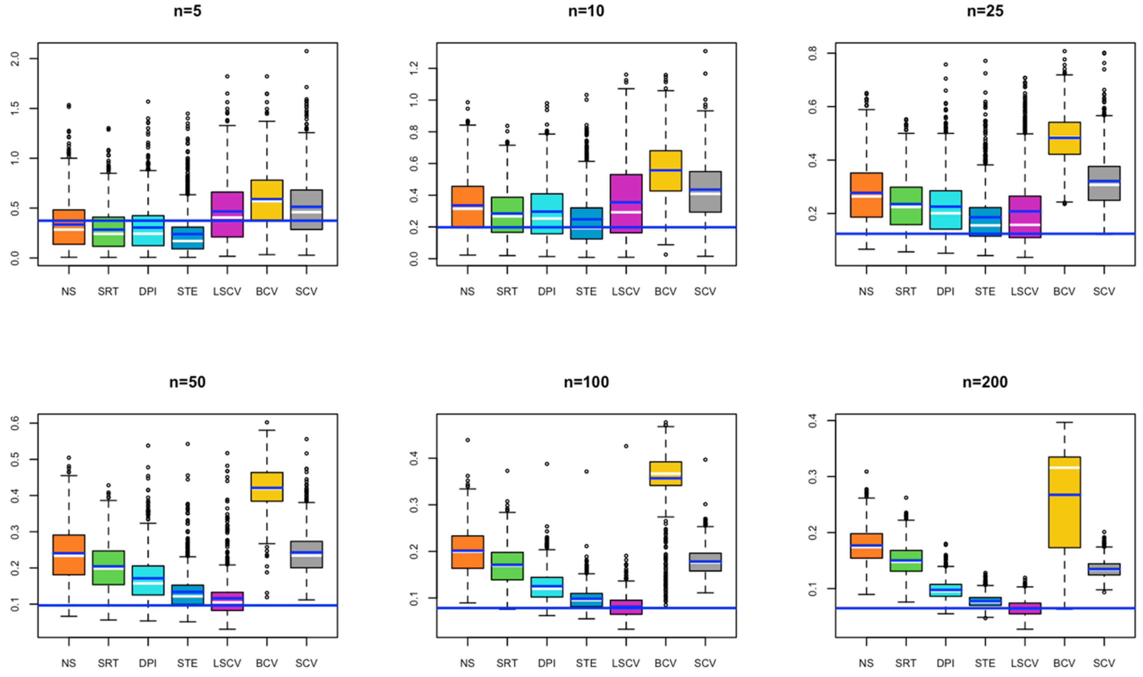
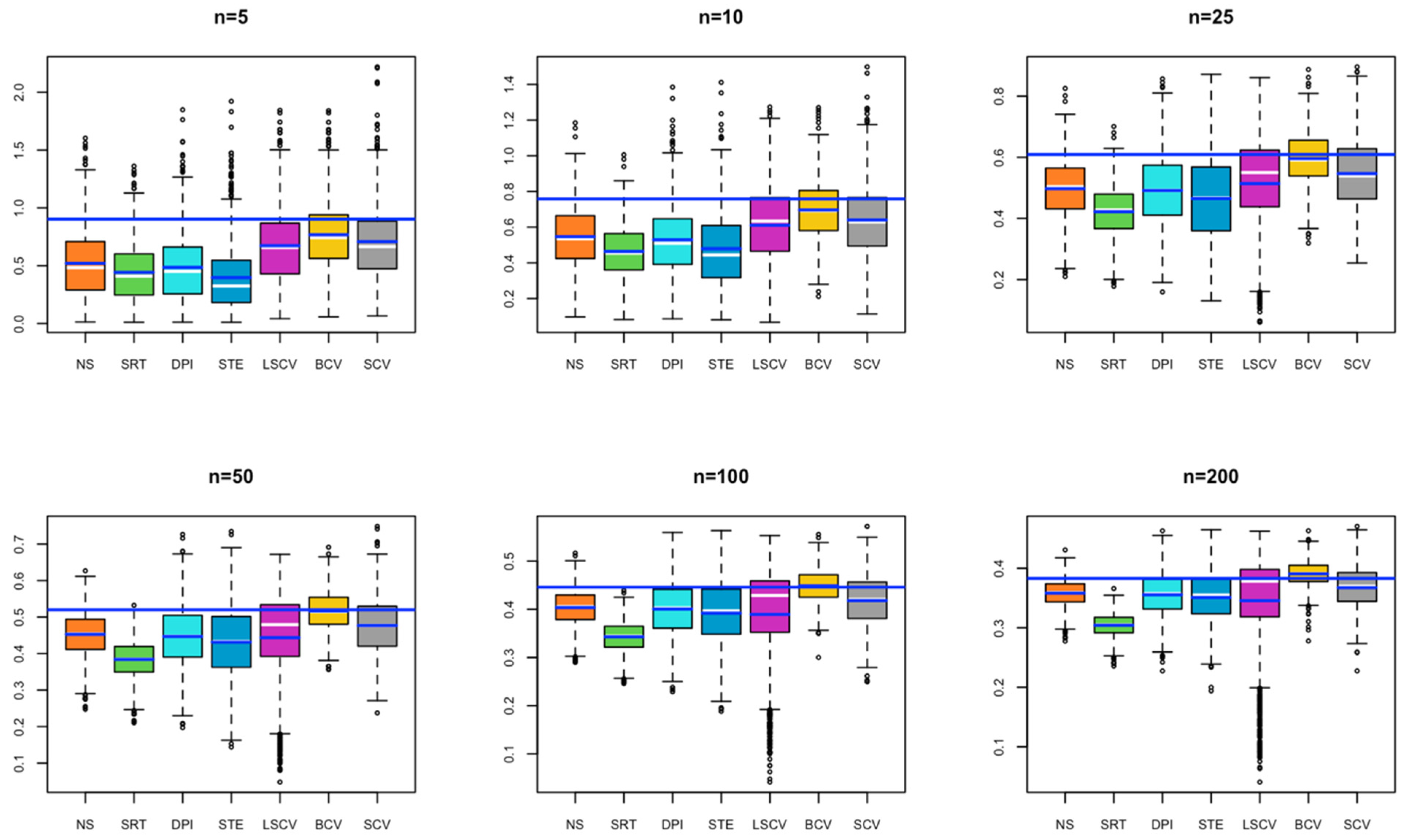
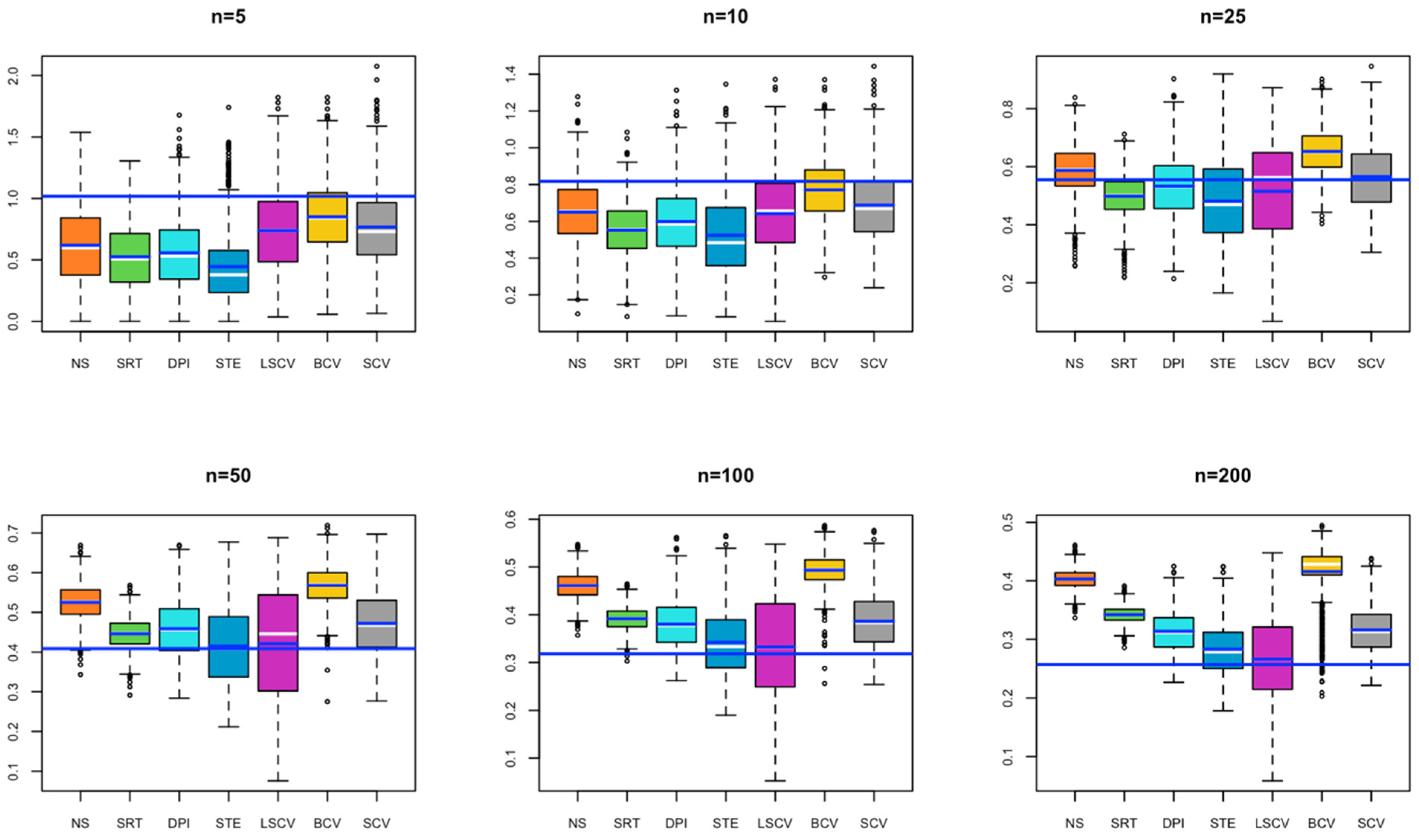
• In Model 1, all estimated bandwidths for small sample size remained below the optimal bandwidth. It is seen that as the sample size increases, the value obtained by the BCV method approaches the optimal bandwidth. In contrast, the bandwidth estimated by the SRT method remains below the optimal bandwidth for each simulated sample size. It may cause under smoothing problems if used in KDE (Figure 1).
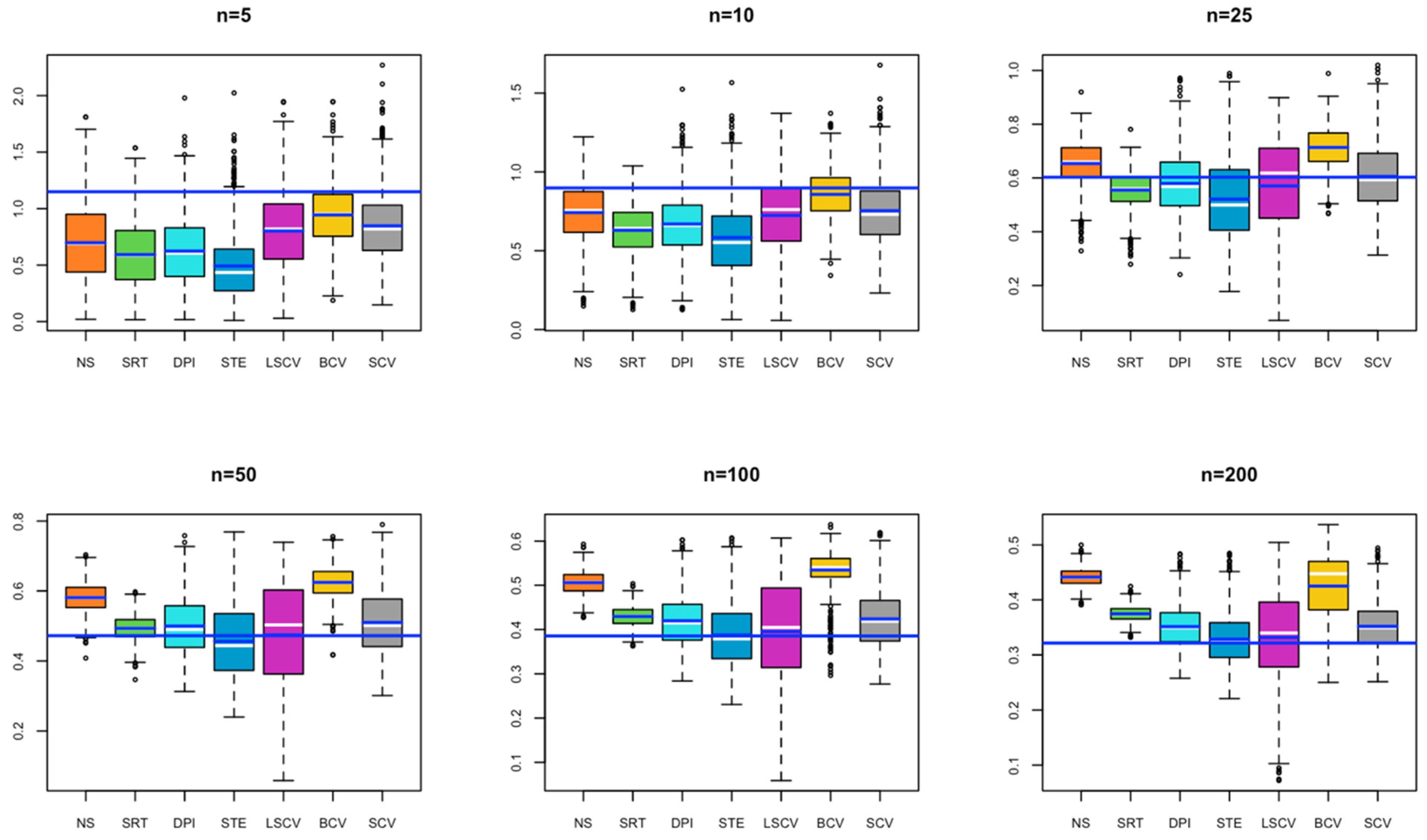
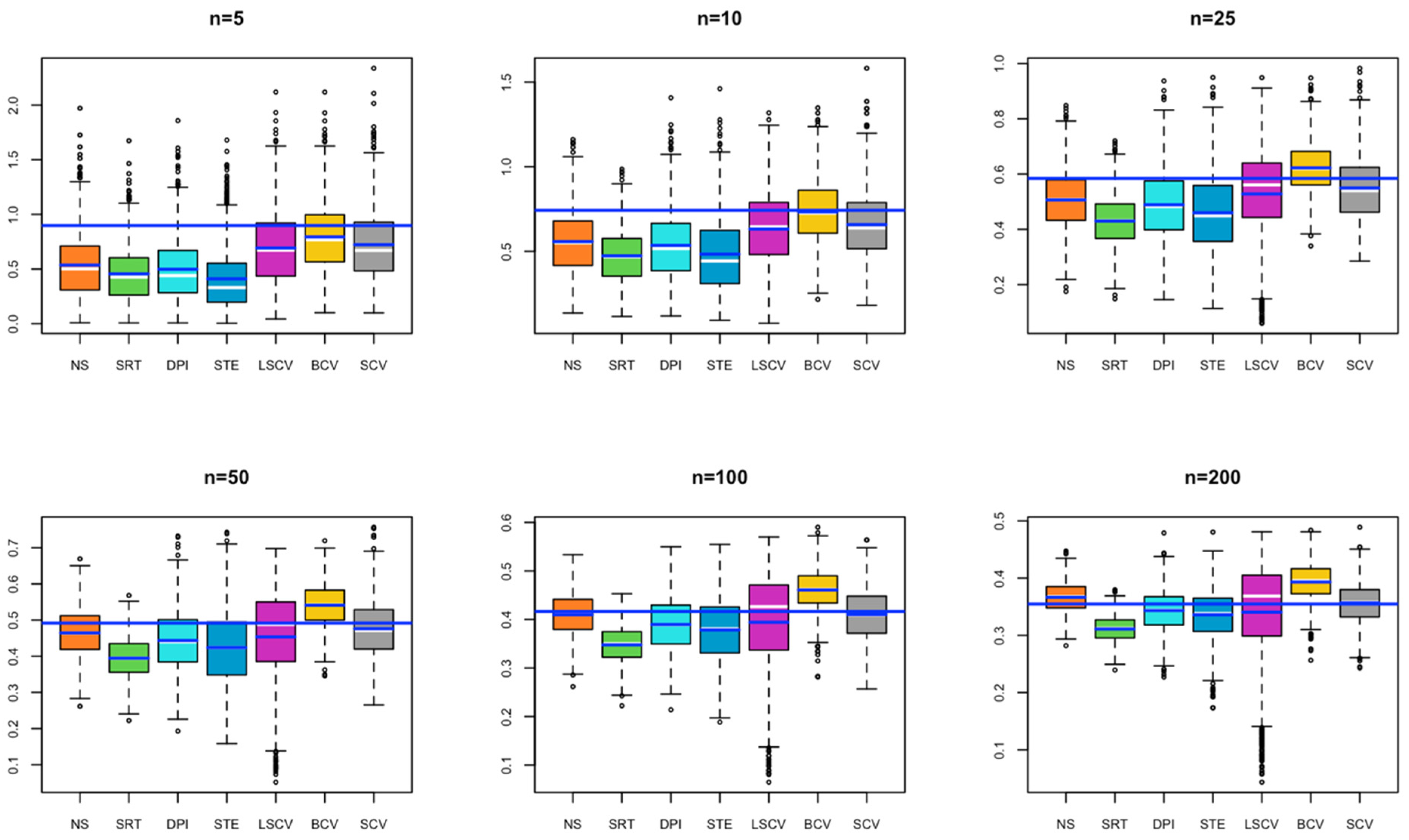
• In Model 2, for small sample sizes (n = 5, 10), BCV and SCV occur close to the optimal bandwidth; as the sample size increases, the SCV method is observed to be the closest to the optimal bandwidth (Figure 2).
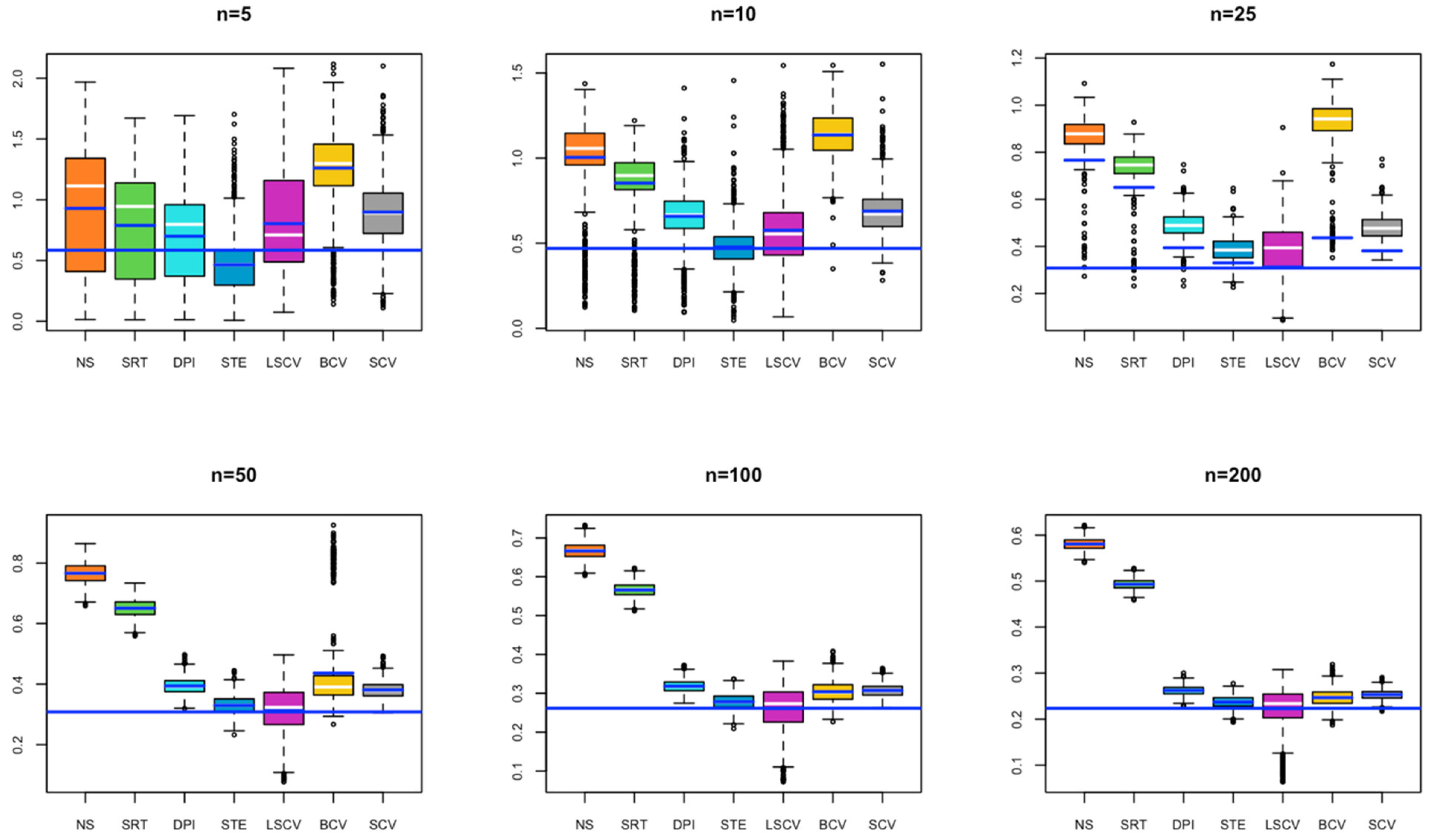
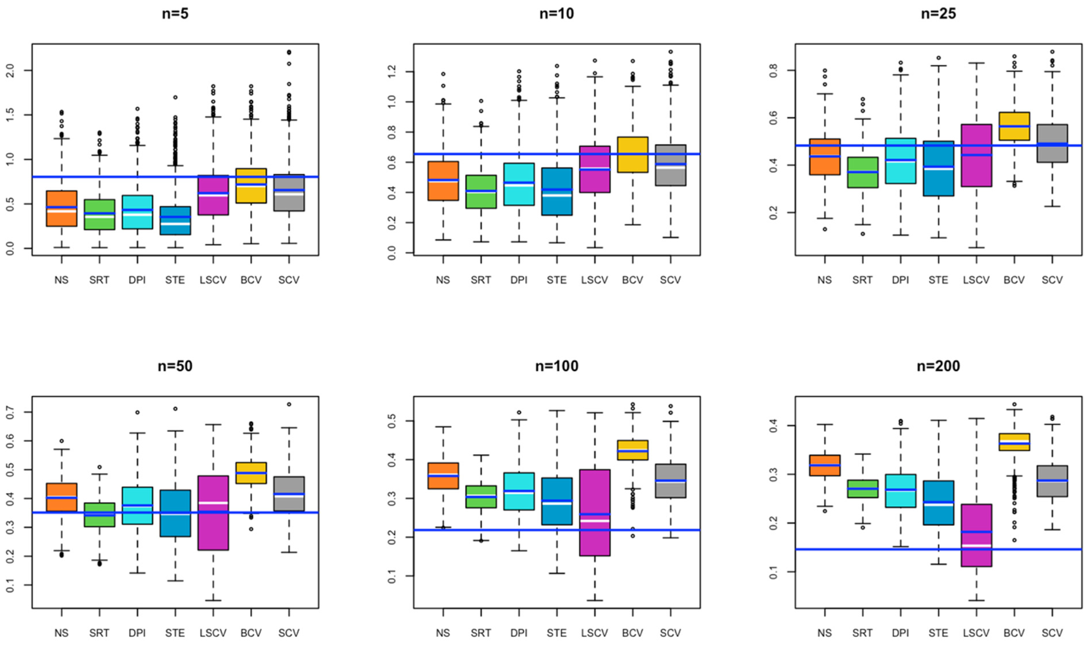
• In Model 3, for a small sample size, the bandwidths estimated by NS, SRT, DPI, STE, and LSCV methods give results close to the optimal bandwidth; as the sample size increases, the bandwidth value estimated by LSCV becomes the closest estimate to the optimal bandwidth (Figure 3).
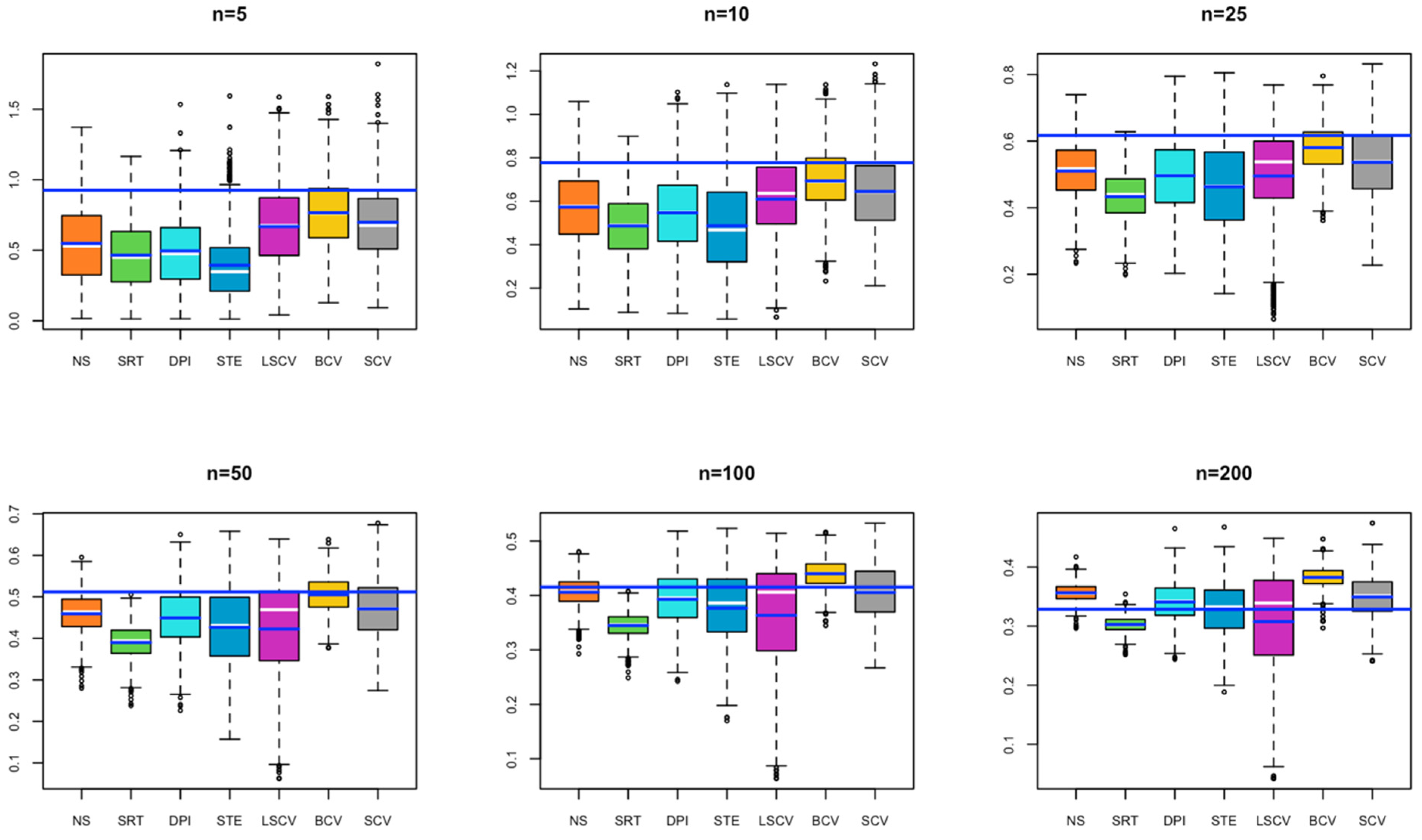
• In Model 4, for small sample size, the bandwidth estimates estimated by BCV, LSCV, and SCV methods give results close to the optimal bandwidth; as the sample size increases, the bandwidth value estimated by LSCV overlaps with the optimal bandwidth value (Figure 4).
• In Model 5, for a small sample size, the bandwidth estimated by the BCV method captures the closest value to the optimal bandwidth; as the sample size increases, the bandwidth values estimated by SRT, DPI, STE, LSCV, and SCV overlap with the optimal bandwidth value (Figure 5).
• In Model 6, in all cases, the bandwidth estimate by the LSCV method captures the optimal bandwidth value, with the STE bandwidth method following the LSCV bandwidth method (Figure 6).
• In Model 7, for a small sample size, although the bandwidth estimate closest to the optimal bandwidth is BCV, as the sample size increases, the bandwidth value estimated by LSCV approaches the optimal bandwidth value (Figure 7).
• In Model 8, for a small sample size, although BCV is the bandwidth estimate closest to the optimal bandwidth, as the sample size increases, the bandwidths estimated by SCV get closer to the optimal bandwidth value (Figure 8).

Furthermore, density plots of the kernel density estimates, based on the simulation results for each distribution, sample size, and bandwidth method, are provided in the supplementary files as Figures S2–S9. We can summarize the results from these figures as follows:

• In Figure S2, for small sample sizes, NS, SRT, DPI, and STE exhibit under smoothing; while as the sample size increases, all bandwidths tend to over smooth.
• In Figure S3, for small sample sizes, SRT, DPI, and STE exhibit under smoothing; while as the sample size increases, all bandwidths tend to over smooth.
• In Figure S4, for small sample sizes, SRT and STE exhibit under smoothing. As the sample size increases, DPI and LCSV also tend to under smooth.
• In Figure S5, for small sample sizes, NS, SRT, DPI, and STE exhibit under smoothing.
• In Figure S6, for small sample sizes, SRT, DPI, and STE exhibit under smoothing; while as the sample size increases, all bandwidths tend to over smooth.
• In Figure S7, for small sample sizes, SRT and DPI exhibit under smoothing; while as the sample size increases, all bandwidths tend to over smooth.
• In Figure S8, as the sample size increases, all bandwidths tend to over smooth.
• In Figure S9, for small sample sizes, NS, SRT, DPI, and STE exhibit under smoothing; while as the sample size increases, all bandwidths tend to over smooth.

5. Application of Real Data

In this section, the considered bandwidth selectors in the previous section are applied to a real dataset. Using the daily average values of the 2022 wind speed (meter/s) in the Kepsut district of the Balıkesir province, it is intended to estimate the monthly wind speed distribution with the KDE method. During this analysis, wind speed data consisting of the 2022 daily average wind speed records in Balıkesir-Kestup, measured and recorded by the Turkish State Meteorological Service, have been used [41].

Firstly, in order to visualize the data structure, boxplots were created for each of the 12 months (Figure 9). The bandwidths that can be used for KDE of monthly wind speed distributions based on the simulation results can now be interpreted: January, February, May, and December look to have skewed distribution. In this case, the SCV method is preferred for estimating bandwidth for these months. On the other hand, April, September, and October are close to normal distribution, so the BCV method is preferred for estimating bandwidth for these months. June and July’s distribution looks to have a skewed bimodal normal mixture. In that case again, the SCV may be a better solution to estimate the bandwidth. If the March and August distribution is accepted as bimodal, again, the most suitable bandwidth selection method will be the SCV.

The wind speed dataset for the Kepsut Balıkesir region in 2022 was divided into monthly segments. For each month, seven distinct Kernel Density Estimates (KDEs) were computed using seven distinct bandwidth calculation methods. The resulting bandwidth estimates and KDE plots are presented in Figure 9 and

Table 3. Estimates of bandwidths by various methods for monthly wind speed data.

Months	NS	SRT	DPI	STE	LCSV	BCV	SCV
January	0.591	0.697	0.457	0.297	0.110	1.049	0.614
February	0.830	0.978	0.682	0.598	0.679	1.050	0.687
March	0.723	0.851	0.692	0.625	0.806	0.914	0.707
April	0.710	0.836	0.691	0.615	0.701	0.911	0.717
May	0.591	0.697	0.487	0.398	0.438	0.752	0.491
June	0.642	0.756	0.527	0.409	0.433	0.813	0.524
July	0.361	0.425	0.411	0.388	0.457	0.457	0.428
August	0.685	0.806	0.633	0.554	0.685	0.866	0.642
September	0.642	0.756	0.512	0.457	0.538	0.876	0.532
October	0.541	0.637	0.687	0.698	0.802	0.803	0.791
November	0.518	0.610	0.587	0.560	0.656	0.655	0.613
December	0.507	0.597	0.369	0.221	0.184	0.862	0.453

respectively.

Another striking point is that while some bandwidths (mostly BCV) shown in pink in Table 3 cause over smoothing compared to the others; some of the bandwidths shown in blue (most STE) may cause under smoothing. Clearly, one can see that when h is too small (the magenta curve) in January and December (Table 3; Figure 10), there are many wiggly structures on the density curve. This is a signature of under smoothing. On the other hand, according to the results obtained in the application, the BCV bandwidth selection method generally caused over smoothing in the month variables, giving higher bandwidth results compared to the other six methods. The STE bandwidth selection method created under smoothing in the month variables, giving generally smaller bandwidth results compared to the other six methods (Table 3; Figure 10).

6. Results

In this study, optimum bandwidths used in the KDEs obtained for different sample sizes taken from normal mixing densities with simulation application, and seven bandwidth selection methods were compared using MSE and Bias of these bandwidth selection methods.

According to the simulation results:

• Bandwidths obtained by the NS selection method give the closest results to the optimal bandwidth at low sample size at kurtotic unimodal density and at high sample size at trimodal density.
• The SRT bandwidth selection method does not approach optimal bandwidth at any of the normal mixing densities.
• The DPI bandwidth selection method does not approach optimal bandwidth at any of the normal mixing densities.
• The STE bandwidth selection method gives the closest result to the optimum bandwidth for kurtotic unimodal and separated bimodal density functions at a low sample size.
• The LSCV bandwidth selection method gives the closest result to the optimum bandwidth for large sample sizes in kurtotic unimodal, outlier, separated bimodal and skewed bimodal density functions.
• The BCV bandwidth selection method at all sample sizes at standard normal density; outlier, skewed bimodal, and trimodal density gives the closest result to optimal bandwidth at a small sample size.
• The SCV bandwidth selection method gives the closest result to the optimal bandwidth for all other sample sizes except for a small sample size at skewed unimodal density.

With real data application, seven bandwidth selection methods were compared by obtaining the kernel density estimates of the Kepsut, Balıkesir region variables.

According to the actual data application results:

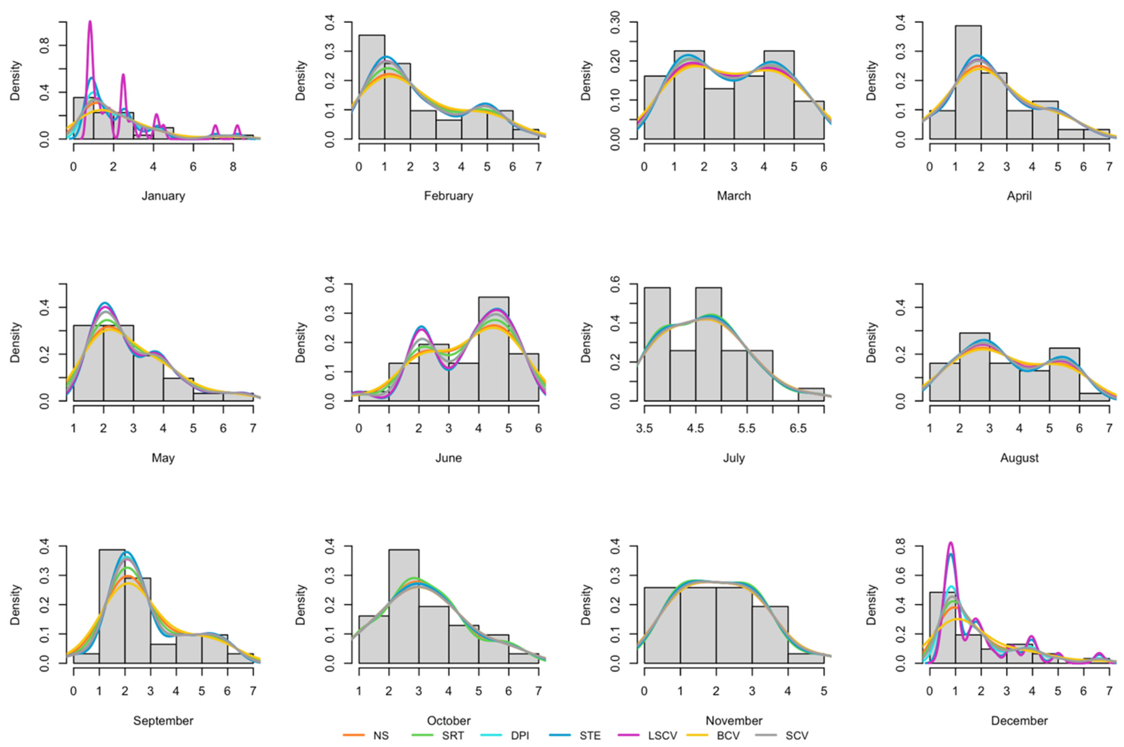
• The BCV bandwidth selection methods have oversmoothed, resulting in high bandwidth in most of the months.
• STE and some of the LSCV bandwidth selection methods have incomplete smoothing, resulting in small bandwidth in some variables.

Although significant improvements have been made recently in bandwidth selectors in many simulation studies examined, these selectors do not perform satisfactorily in all cases. That is, although it is not possible to determine a single best bandwidth selector for all PDFs, the shape and structure of the density to be estimated also have a great influence on the bandwidth selection methods. Therefore, estimates for various bandwidths must be obtained.

7. Conclusions

Throughout this paper, we have presented a detailed study that makes a substantial contribution to the field by offering a comprehensive analysis of bandwidth selection methodologies in the ubiquitous context of kernel density estimation. We have applied a multifaceted approach that combines rigorous data analysis and theoretical principles. While prior research has compared bandwidth selection methods, our study not only specifically provides clear guidelines for practitioners but also crucially applies these methods to wind speed data from the Balıkesir, Kepsut region for the year 2022.

Our work bridges the gap between general kernel density estimation techniques and their practical application to wind speed data, which is essential for renewable energy research. By focusing on monthly kernel density estimations, we provide a detailed temporal view of wind speed variations that offers unique insights compared to broader time-scale analyses. Additionally, our use of simulation studies with various parameter choices and sample sizes ranging from small to large ensures the theoretical robustness and practical applicability of our findings.

In particular, our research reveals the suitability of the SCV method for estimating bandwidth in our specific dataset. This nuanced insight may not have been apparent in other contexts or with different datasets, underscoring the relevance and timeliness of our work. In conclusion, our study serves as a consolidated source of information on bandwidth selection, offering an integrated understanding for those in the field of renewable energy research.

Future work:

• Geographical viability and terrain analysis: To validate the robustness of the SCV method, future research should extend its investigation across diverse geographical regions and terrain types, considering variations in wind speed data originating from different climatic conditions. Such an approach will help in comprehensively assessing the method’s applicability and ensuring its adaptability across varied environmental contexts.
• Adaptive algorithms and time-series analysis: Leveraging advancements in machine learning and artificial intelligence, a promising avenue for research involves the development of adaptive algorithms capable of dynamically selecting the most suitable bandwidth method based on real-time wind speed data. Additionally, a more detailed time-series analysis should be pursued to uncover diurnal, weekly, and seasonal patterns in wind speed data, further evaluating the performance of bandwidth selectors on these shorter time scales.
• Hybrid bandwidth selection approaches and comparative analysis: Building on the identification of the SCV method as optimal, future investigations can delve into refining its implementation or combining it with other bandwidth methods to create hybrid approaches. These approaches may integrate techniques such as weighted averages, adaptive selection, iterative refinement, data segmentation, bootstrap combination, or a machine learning approach to enhance precision. Furthermore, ongoing studies should continually compare established methods with any emerging contenders to ensure that the most accurate wind speed distribution predictions are achieved in the ever-evolving landscape of technological and mathematical advancements.

References

1. Foyhirun, C.; Kongkitkul, D.K.; Ekkawatpanit, C. Performance of Global Climate Model (GCMs) for wind data analysis. E3S Web Conf. 2019, 117, 3–7. [Google Scholar] [CrossRef]
2. Donk, P.; Van Uytven, E.; Willems, P. Statistical methodology for on-site wind resource and power potential assessment under current and future climate conditions: A case study of Suriname. SN Appl. Sci. 2019, 1, 846. [Google Scholar] [CrossRef]
3. Shi, H.; Dong, Z.; Xiao, N.; Huang, Q. Wind Speed Distributions Used in Wind Energy Assessment: A Review. Front. Energy Res. Wind Energy 2021, 9, 769920. [Google Scholar] [CrossRef]
4. Rosenblatt, M. Remarks on Some Nonparametric Estimates of a Density Function. Ann. Stat. 1956, 27, 832–837. [Google Scholar] [CrossRef]
5. Parzen, E. On the estimation of a probability density function and the mode. Ann. Stat. 1962, 33, 1065–1076. [Google Scholar] [CrossRef]
6. Silverman, B.W. Density Estimation for Statistics and Data Analysis, 1st ed.; Chapman and Hall: London, UK, 1986; pp. 1–48. [Google Scholar]
7. Terrell, G.R. The Maximal Smoothing Principle in Density Estimation. J. Am. Stat. Assoc. 1990, 85, 470–477. [Google Scholar] [CrossRef]
8. Gramacki, A. Nonparametric Kernel Density Estimation and Its Computational Aspects; Springer: Cham, Switzerland, 2018. [Google Scholar]
9. Rudemo, M. Empirical choice of histograms and kernel density estimators. Scand. Stat. Theory Appl. 1982, 9, 65–78. [Google Scholar]
10. Bowman, A.W. An alternative method of cross-validation for the smoothing of density estimates. Biometrika 1984, 71, 353–360. [Google Scholar] [CrossRef]
11. Scott, D.; Terrell, G. Biased and unbiased cross-validation in density estimation. J. Am. Stat. Assoc. 1987, 82, 1131–1146. [Google Scholar] [CrossRef]
12. Sheather, S.J.; Jones, M.C. A Reliable Data-Based Bandwidth Selection Method for Kernel Density Estimation. J. R. Stat. Soc. Ser. B Methodol. 1991, 53, 683–690. [Google Scholar] [CrossRef]
13. Cao, R.; Cuevas, A.; Gonzalez Manteiga, W. A comparative study of several smoothing methods in density estimation. Comput. Statist. Data Anal. 1994, 17, 153–176. [Google Scholar] [CrossRef]
14. Harpole, J.K. How Bandwidth Selection Algorithms Impact Exploratory Data Analysis Using Kernel Density Estimation. Master’s Thesis, University of Kansas, Lawrence, KS, USA, 2013. [Google Scholar]
15. Harpole, J.K.; Woods, C.M.; Rodebaugh, T.L.; Levinson, C.A.; Lenze, E.J. How bandwidth selection algorithms impact exploratory data analysis using kernel density estimation. Psychol. Methods 2014, 9, 428–443. [Google Scholar] [CrossRef] [PubMed]
16. Demir, S. Adaptive kernel density estimation with generalized least square cross-validation. Hacet. J. Math. Stat. 2019, 48, 616–625. [Google Scholar] [CrossRef]
17. Wallin, G.; Häggström, J.; Wiberg, M. How Important is the Choice of Bandwidth in Kernel Equating? Appl. Psychol. Meas. 2021, 45, 518–535. [Google Scholar] [CrossRef] [PubMed]
18. Karakoç, Ş. Çekirdek Düzgünleştirmesiyle Yoğunluk Fonksiyonu Tahmininde Bant Genişliği Seçim Yöntemlerinin Karşılaştırılması. Master’s Thesis, Gazi University, Ankara, Turkey, 2023. [Google Scholar]
19. Henderson, D.J.; Papadopoulos, A.; Parmeter, C.F. Bandwidth selection for kernel density estimation of fat-tailed and skewed distributions. J. Stat. Comput. Simul. 2023, 93, 2110–2135. [Google Scholar] [CrossRef]
20. Dokur, E.; Kurban, M. Wind Speed Potential Analysis Based on Weibull Distribution. Balk. J. Electr. Comput. Eng. 2015, 3, 231–235. [Google Scholar] [CrossRef]
21. Miao, S.; Xie, K.; Yang, H.; Karki, R.; Tai, H.-M.; Chen, T. A mixture kernel density model for wind speed probability distribution estimation. Energy Convers. Manag. 2016, 126, 1066–1083. [Google Scholar] [CrossRef]
22. Hu, B.; Li, Y.; Yang, H.; Wang, H. Wind speed model based on kernel density estimation and its application in reliability assessment of generating systems. J. Mod. Power Syst. Clean Energy 2017, 5, 220–227. [Google Scholar] [CrossRef]
23. Citakoglu, H.; Aydemir, A. Determination of Monthly Wind Speed of Kayseri Region with Gray Estimation Method. In Proceedings of the 2019 IEEE Jordan International Joint Conference on Electrical Engineering and Information Technology (JEEIT), Amman, Jordan, 9–11 April 2019. [Google Scholar] [CrossRef]
24. Han, Q.; Ma, S.; Wang, T.; Chu, F. Kernel density estimation model for wind speed probability distribution with applicability to wind energy assessment in China. Renew. Sust. Energ. Rev. 2019, 115, 109387. [Google Scholar] [CrossRef]
25. Zhang, L.; Xie, L.; Han, Q.; Wang, Z.; Huang, C. Probability Density Forecasting of Wind Speed Based on Quantile Regression and Kernel Density Estimation. Energies 2020, 13, 6125. [Google Scholar] [CrossRef]
26. An, X.-Y.; Yan, Z.; Jia, J.-M. A new distribution for modeling wind speed characteristics and evaluating wind power potential in Xinjiang, China. Energy Sources A Recovery Util. Environ. Eff. 2020, 1, 1556–7036. [Google Scholar] [CrossRef]
27. He, Y.-L.; Ye, X.; Huang, D.-F.; Huang, J.Z.; Zhai, J.-H. Novel kernel density estimator based on ensemble unbiased cross-validation. Inf. Sci. 2021, 581, 327–344. [Google Scholar] [CrossRef]
28. Jabbar, R.I. Statistical Analysis of Wind Speed Data and Assessment of Wind Power Density Using Weibull Distribution Function (Case Study: Four Regions in Iraq). Phys. Conf. Ser. 2021, 1804, 012010. [Google Scholar] [CrossRef]
29. Liu, L.; Wang, J.; Li, J.; Wei, L. Estimation of wind speed distribution with time window and new kernel function. J. Renew. Sustain. Energy 2022, 14, 053307. [Google Scholar] [CrossRef]
30. Wahbah, M.; Mohandes, B.; EL-Fouly, T.H.M.; El Moursi, M.S. Unbiased cross-validation kernel density estimation for wind and PV probabilistic modelling. Energy Convers. Manag. 2022, 266, 115811. [Google Scholar] [CrossRef]
31. Zhou, S.; Yang, Y.; Gao, Z.; Xi, X.; Duan, Z.; Li, Y. Estimating vertical wind power density using tower observation and empirical models over varied desert steppe terrain in northern China. Atmos. Meas. Tech. 2022, 15, 757–773. [Google Scholar] [CrossRef]
32. Silveira, F.; Gomes-silva, F.; Brito, C.; Jale, J.; Gusmão, F.; Xavier-júnior, S.; Rocha, J. Modelling wind speed with a univariate probability distribut ion depending on two baseline functions. Hacet. J. Math. Stat. 2023, 52, 808–827. [Google Scholar] [CrossRef]
33. Wand, M.P.; Jones, M.C. Kernel Smoothing, 1st ed.; Chapman & Hall: New York, NY, USA, 1995. [Google Scholar]
34. Yolsal, H. Parametrik Olmayan Yoğunluk Tahmincileri ve Regresyon Analizi (Birinci Baskı); Detay Yayıncılık: Ankara, Turkey, 2017. [Google Scholar]
35. Sheather, S.J. Density estimation. Stat. Sci. 2004, 19, 558–597. [Google Scholar] [CrossRef]
36. Hall, P. Large sample optimality of least squares cross-validation in density estimation. Ann. Stat. 1983, 11, 1156–1174. [Google Scholar] [CrossRef]
37. Park, B.; Marron, J. Comparison of data-driven bandwidth selectors. J. Am. Stat. Assoc. 1990, 85, 66–72. [Google Scholar] [CrossRef]
38. Jones, C.; Marron, J.; Sheather, S. Progress in data-based bandwidth selection for kernel density estimation. Comput. Stat. 1996, 11, 337–381. [Google Scholar]
39. Marron, S.; Wand, M. Exact mean integrated squared error. Ann. Stat. 1992, 20, 712–736. [Google Scholar] [CrossRef]
40. Cran.r-project. 2022. Available online: https://cran.rproject.org/web/packages/ks/ks.pdf (accessed on 10 January 2022).
41. Turkish State Meteorological Service. Available online: https://mevbis.mgm.gov.tr/mevbis/ui/index.html#/Workspace (accessed on 8 September 2023).
Figure 1. Box plots display the distribution of 1000 bandwidth estimates obtained from the simulation study for the Gaussian distribution. The horizontal line represents the optimal bandwidth value.
Mathematics 11 04478 g001
Figure 2. Box plots display the distribution of 1000 bandwidth estimates obtained from the simulation study for the skewed unimodal distribution. The horizontal line represents the optimal bandwidth value.
Mathematics 11 04478 g002
Figure 3. Box plots display the distribution of 1000 bandwidth estimates obtained from the simulation study for the kurtotic unimodal distribution. The horizontal line represents the optimal bandwidth value.
Mathematics 11 04478 g003
Figure 4. Box plots display the distribution of 1000 bandwidth estimates obtained from the simulation study for the outlier distribution. The horizontal line represents the optimal bandwidth value.
Mathematics 11 04478 g004
Figure 5. Box plots display the distribution of 1000 bandwidth estimates obtained from the simulation study for the bimodal normal mixture distribution. The horizontal line represents the optimal bandwidth value.
Mathematics 11 04478 g005
Figure 6. Box plots display the distribution of 1000 bandwidth estimates obtained from the simulation study for the separated bimodal normal mixture distribution. The horizontal line represents the optimal bandwidth value.
Mathematics 11 04478 g006
Figure 7. Box plots display the distribution of 1000 bandwidth estimates obtained from the simulation study for the skewed bimodal normal mixture distribution. The horizontal line represents the optimal bandwidth value.
Mathematics 11 04478 g007
Figure 8. Box plots display the distribution of 1000 bandwidth estimates obtained from the simulation study for the trimodal normal mixture distribution. The horizontal line represents the optimal bandwidth value.
Mathematics 11 04478 g008
Figure 9. Boxplot of the 2022 Kepsut region wind data set by month.
Mathematics 11 04478 g009
Figure 10. Kernel density estimates of the 2022 Balıkesir, Kepsut region wind data set by month, obtained with bandwidths calculated according to seven different methods.
Mathematics 11 04478 g010