Analysis of Within-Host Mathematical Models of Toxoplasmosis That Consider Time Delays

Abstract

In this paper, we investigate two within-host mathematical models that are based on differential equations. These mathematical models include healthy cells, tachyzoites, and bradyzoites. The first model is based on ordinary differential equations and the second one includes a discrete time delay. We found the models’ steady states and computed the basic reproduction number ${\mathcal{R}}_0$. Two equilibrium points exist in both models: the first is the disease-free equilibrium point and the second one is the endemic equilibrium point. We found that the initial quantity of uninfected cells has an impact on the basic reproduction number ${\mathcal{R}}_0$. This threshold parameter also depends on the contact rate between tachyzoites and uninfected cells, the contact rate between encysted bradyzoite and the uninfected cells, the conversion rate from tachyzoites to bradyzoites, and the death rate of the bradyzoites- and tachyzoites-infected cells. We investigated the local and global stability of the two equilibrium points for the within-host models that are based on differential equations. We perform numerical simulations to validate our analytical findings. We also demonstrated that the disease-free equilibrium point cannot lose stability regardless of the value of the time delay. The numerical simulations corroborated our analytical results.

1. Introduction

Toxoplasmosis is caused by the parasite Toxoplasma gondii, and is one of the most common parasitic infections of humans and other animals. Approximately one-third of people have been exposed to the parasite, which is present throughout the world [1]. T. gondii has a facultative heterogeneous life cycle. A series of intricate, independently controlled processes make up the toxoplasma invasion process [2]. All warm-blooded creatures, including the majority of livestock and humans, are most likely intermediate hosts. Family Felidae individuals, such as household cats, are the definitive hosts [3]. In developing fetuses and immune-compromised patients, toxoplasma can cause serious and fatal diseases (such as encephalitis, retinitis, and myocarditis). Although there are already medicines that can treat toxoplasma infections, they are not well-received, have unfavorable side effects, and cannot treat toxoplasma infections that have existed for a long period. Additionally, resistance to several of these medications has lately been identified [4,5,6].

The intricate life cycle of toxoplasma includes an asexual cycle in intermediate hosts and a sexual cycle in its definitive feline hosts [7]. When an infected cat sheds oocysts, the environment becomes contaminated [8]. Mammals and birds can consume these oocysts and subsequently develop the infection [9,10]. The secondary hosts might also become infected by eating an infected organism [3]. Toxoplasma can be transmitted between intermediate hosts in two ways: vertically (mother–embryo) or horizontally (carnivorism). Infectious phases of the T. gondii life cycle include tachyzoites, bradyzoites enclosed in tissue cysts, and sporozoites contained in sporulated oocysts. Within a host, T. gondii occurs in two interconvertible stages: bradyzoites and tachyzoites [3,11,12]. Both intermediate and definitive hosts are contagious to all three stages, and they can become infected with T. gondii primarily by ingesting bradyzoite cysts [13,14]. Tachyzoites can also be transferred from a mother to her young through their milk in a number of hosts [2,15]. This means that T. gondii can spread from definitive and intermediate hosts as well as from intermediate to definitive hosts [2].

Bradyzoites exist in a dormant, slow-growing, and encysted form within a host cell [2], whereas tachyzoites reproduce quickly and are ready to infect and cause disease [3,16]. Infections with bradyzoite-containing cysts occur after consuming uncooked meat [16]. The walls of the cysts containing bradyzoite are digested in the host’s stomach after they have been consumed by the host. The gastric-condition-resistant bradyzoites in the stomach will subsequently enter the small intestine epithelial cells of the host and transform into tachyzoites there [3,16]. The acute infection phase is brought on by tachyzoites, which spread throughout the body. Tachyzoites multiply inside parasitophorous vacuoles (PVs), egress, and then infect neighboring cells, infecting the majority of nucleated cells. A powerful host immune response is triggered by these tachyzoites, and the majority of the parasites are destroyed. However, some tachyzoites manage to endure the devastation and turn back into the latent bradyzoites stage within host cells [16]. If there is not a sufficient immune response, tachyzoites will keep multiplying and destroying tissue, which can have detrimental and even fatal consequences. However, tachyzoites can cause immune-mediated cellular damage because of the inflammatory immunological response they trigger. As a result, for toxoplasma to establish a chronic infection, a delicate balance between activating and evading the immune response is essential [16]. Numerous in vivo and in vitro conditions can affect the interconversion of tachyzoites and bradyzoites [3].

Toxoplasmosis has developed into an extensively dispersed disease due to how simple it is to transmit to intermediate hosts. A persistent infection that can withstand both the host’s immune system and all known anti-toxoplasmosis drugs is possible when the parasite penetrates the host and develops a powerful mechanism to modify its host cell and to become a chronic infection. To reproduce inside a host cell, escape immune responses, and experience bradyzoite development, the parasite must successfully modify its host [2]. According to current research from many laboratories, toxoplasma and its host communicate in two main ways. The first type, which is essential for bradyzoite or parasite multiplication, does not seem to vary between different toxoplasma strains. On the other hand, the second type of communication between toxoplasma and its host differs among distinct toxoplasma strains [16].

Previous works have studied toxoplasmosis dynamics in human and cat populations by using mathematical models based on ordinary differential equations [17,18,19,20,21,22,23,24]. For instance, a mathematical model based on a nonlinear system of ordinary differential equations has been used to describe the co-infection dynamics of malaria and toxoplasmosis in the human and feline populations [25]. Recently, few studies have investigated the effects of discrete time delays on the dynamics of toxoplasmosis [26,27].

In this paper, we investigate the within-host dynamics of toxoplasmosis by means of mathematical models that are based on ordinary differential equations (ODEs) and delay differential equations (DDEs). These mathematical models are simplified approximations of the real world and provide additional insight into the dynamics. These models consider healthy cells, tachyzoites, and bradyzoites. The first model is based on ordinary differential equations and the second one includes a discrete time delay. We find the models’ steady states and compute the basic reproduction number ${\mathcal{R}}_0$. We investigate the local and global stability of the equilibrium points for the within-host models. We perform numerical simulations to provide additional support to the theoretical findings. We demonstrate that the stability of the disease-free equilibrium point is not affected by the discrete time delay. The paper is organized as follows: In Section 2, we present the mathematical model. Section 3 is devoted to stability analysis of the steady states and computing ${\mathcal{R}}_0$. Section 4 contains numerical simulations of different scenarios. We perform useful sensitivity analysis in Section 5. In Section 6, we modify the first model by adding a discrete time delay and analyzing the stability of the steady states. Finally, Section 7 and Section 8 are devoted to numerical simulations that support our theoretical results and the conclusions.

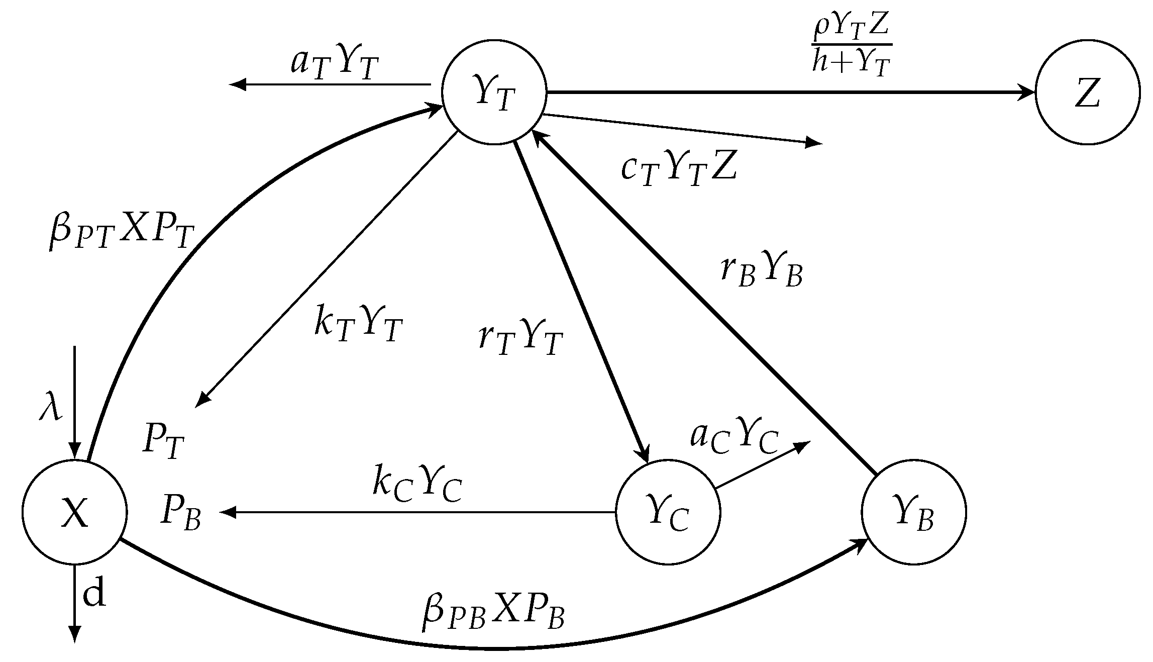
2. Mathematical Model for Toxoplasmosis Within-Host Dynamics

In this section, we will start studying a mathematical model for toxoplasmosis within-host dynamics that was developed in [3]. This compartmental model was designed by the authors to explain the invasion dynamics of within-host T. gondii. The proposed model deals with seven state variables, which are the following:

$$\left\{\begin{array}{cc}X\hfill & \mathrm{The}\mathrm{number}\mathrm{of}\mathrm{uninfected}\mathrm{cells}\hfill \\ Y_T\hfill & \mathrm{The}\mathrm{number}\mathrm{of}\mathrm{tachyzoite}-\mathrm{infected}\mathrm{cells}\hfill \\ Y_B\hfill & \mathrm{The}\mathrm{number}\mathrm{of}\mathrm{early}-\mathrm{stage}-\mathrm{bradyzoite}-\mathrm{containing}\mathrm{cells}\hfill \\ Y_C\hfill & \mathrm{The}\mathrm{number}\mathrm{of}\mathrm{encysted}-\mathrm{bradyzoite}-\mathrm{containing}\mathrm{cells}\hfill \\ P_T\hfill & \mathrm{The}\mathrm{number}\mathrm{of}\mathrm{free}\mathrm{tachyzoites}\hfill \\ P_B\hfill & \mathrm{The}\mathrm{number}\mathrm{of}\mathrm{free}\mathrm{bradyzoites}\hfill \\ Z\hfill & \mathrm{The}\mathrm{host}’\mathrm{s}\mathrm{immune}\mathrm{system}’\mathrm{s}\mathrm{effector}\mathrm{cells}.\hfill \end{array}\right.$$

In [3], the authors considered that if there is no infection, then the rate of change in the population of uninfected cells can be expressed by the formula $\dot{X}=\lambda -dX$. Here, $\lambda$ is the constant production rate of the uninfected cells and $1/d$ is the average lifespan of an uninfected cell. When the number of uninfected cells approaches the steady state, the equilibrium point is given by $X_0=\lambda /d$. Free tachyzoite infects uninfected cells at a constant rate ${\beta }_{PT}$, whereas free bradyzoites infect the uninfected cells at a constant rate ${\beta }_{PB}$. Here, both ${\beta }_{PT}$ and ${\beta }_{PB}$ address the efficacy of the invading process and are influenced by a number of factors such as the probability of finding uninfected cells, how quickly the parasites spread to healthy cells and the likelihood that the infection will be successful. The unit of the parameters ${\beta }_{PT}$ and ${\beta }_{PB}$ is given by the number of cells/time [3,28,29,30].

Then, considering all the above factors and parameters, the following model is introduced in [3],

$$\begin{array}{ccc}\dot{X}& \hfill =& d\left(X_0-X\right)-{\beta }_{PT}X{P}_T-{\beta }_{PB}X{P}_B,\hfill \\ \dot{Y_T}& \hfill =& {\beta }_{PT}X{P}_T-c_T{Y}_{T}Z+r_B{Y}_B-a_T{Y}_T-r_T{Y}_T,\hfill \\ \dot{Y_C}& \hfill =& r_T{Y}_T-a_C{Y}_C,\hfill \\ \dot{Y_B}& \hfill =& {\beta }_{PB}X{P}_B-r_B{Y}_B,\hfill \\ \dot{P_T}& \hfill =& k_T{Y}_T-u_T{P}_T,\hfill \\ \dot{P_B}& \hfill =& k_C{Y}_C-u_B{P}_B,\hfill \\ \dot{Z}& \hfill =& \frac{\rho Y_{T}Z}{h+Y_T}-\delta Z.\hfill \end{array}$$

(1)

Model (1) without the removing terms of free tachyzoites and bradyzoites is depicted in Figure 1. The meanings of the parameters of the mathematical model (1) are given in

Table 1. Table of parameters for the toxoplasmosis within-host mathematical model (1).

Parameters	Symbols
Production rate of uninfected cells	$\lambda$
Production rate of the effector cells	$\rho$
The saturation level of the effector cells	h
The removal rate of the immune system response	$\delta$
Conversion rate from the early stage bradyzoites to tachyzoites	$r_B$
Conversion rate from tachyzoites to encysted bradyzoite	$r_T$
The average lifetime of a tachyzoite-infected cell	$1/a_T$
The average lifetime of an encysted-bradyzoite-infected cell	$1/a_C$
The average lifetime of an uninfected cell	$1/d$
Contact rate between free tachyzoites and uninfected cells	${\beta }_{PT}$
Contact rate between free bradyzoite and uninfected cells	${\beta }_{PB}$
Contact rate between tachyzoite-infected cells and effector cells	$c_T$
Free parasite production rate for free tachyzoites and bradyzoites, respectively	$k_T$ and $k_C$
Removing rate for free tachyzoites and bradyzoites, respectively	${\mu }_T$ and ${\mu }_B$

.

Now, taking into account that since tachyzoites reproduce significantly more quickly than bradyzoites, it can be assumed $a_C\ll a_T$ [3,31]. In [3], the authors did not work on the stability analysis of model (1) since they assumed that “The kinetics of free parasites are significantly faster than the kinetics of other processes” on the basis of some recent and previous experiments. As a result, they considered the free tachyzoites and bradyzoites parasites in the equilibrium stage. Then, from the fifth and sixth equations of system (1), one obtains the following two equations

$$P_T={\displaystyle \frac{k_T{Y}_T}{u_T}}\mathrm{and}{P}_B={\displaystyle \frac{k_C{Y}_C}{u_B}}.$$

(2)

Then, using the above two conversions into the first four equations and the last equation from system (1), one obtains the following reduced model with five equations

$$\begin{array}{ccc}\dot{X}& \hfill =& d(X_0-X)-{\beta }_T{Y}_{T}X-{\beta }_B{Y}_{C}X,\hfill \\ \dot{Y_T}& \hfill =& {\beta }_T{Y}_{T}X+r_B{Y}_B-a_T{Y}_T-r_T{Y}_T-c_T{Y}_{T}Z,\hfill \\ \dot{Y_C}& \hfill =& r_T{Y}_T-a_C{Y}_C,\hfill \\ \dot{Y_B}& \hfill =& {\beta }_B{Y}_{C}X-r_B{Y}_B\hfill \\ \dot{Z}& \hfill =& \frac{\rho Y_{T}Z}{h+Y_T}-\delta Z,\hfill \end{array}$$

(3)

where ${\beta }_T={\displaystyle \frac{k_T{\beta }_{PT}}{u_T}}$ and ${\beta }_B={\displaystyle \frac{k_C{\beta }_{PB}}{u_B}}$. All parameters of model (3) are considered to be non-negative and the non-negativity of the solution has been proved in [3]. Therefore, the model can be analyzed in the following biologically feasible region

$$\mathcal{D}=\left\{(X,Y_T,Y_C,Y_B,Z)\in {\mathbb{R}}_{+}^5:X\ge 0,Y_T\ge 0,Y_C\ge 0,Y_B\ge 0,Z\ge 0\right\}.$$

3. Toxoplasmosis Within-Host Mathematical Model

The previous model (3) can be first analyzed assuming that there are no immune system effector cells [3]. Notice that there are natural death rates for the tachyzoite-infected cells ($a_T$) and for the bradyzoite-infected cells ($a_C$). Therefore, assuming that the state variable Z is zero one obtains a simplified mathematical model of four equations that represent the uninfected cells X, tachyzoite-infected cells $Y_T$, early-stage-bradyzoite-containing cells $Y_B$ and encysted-bradyzoite-containing cells $Y_C$. We will proceed to study the dynamics of this simplified toxoplasmosis within-host model in order to obtain a better insight into the more complex toxoplasmosis within-host models (1) and (3).

First, let us present the simplified toxoplasmosis within-host model with four ODEs. This nonlinear model is given by the following system:

$$\begin{array}{ccc}\dot{X}& \hfill =& d(X_0-X)-{\beta }_T{Y}_{T}X-{\beta }_B{Y}_{C}X,\hfill \\ \dot{Y_T}& \hfill =& {\beta }_T{Y}_{T}X+r_B{Y}_B-a_T{Y}_T-r_T{Y}_T,\hfill \\ \dot{Y_C}& \hfill =& r_T{Y}_T-a_C{Y}_C,\hfill \\ \dot{Y_B}& \hfill =& {\beta }_B{Y}_{C}X-r_B{Y}_B.\hfill \end{array}$$

(4)

First, we compute the equilibrium points of model (4). There are two equilibrium points, which are

1.

Disease-free (DFE): $(X^0,Y_T^0,Y_C^0,Y_B^0)=(X_0,0,0,0)$.

2.

Endemic (EE): $(X^{*},Y_T^{*},Y_C^{*},Y_B^{*})$,

where

$$\begin{array}{cc}\hfill X^{*}& =\frac{a_C\left(a_T+r_T\right)}{a_C{\beta }_T+{\beta }_B{r}_T},\hfill \\ \hfill Y_T^{*}& =\frac{d\left(X_0{a}_C{\beta }_T+X_0{\beta }_B{r}_T-a_C{a}_T-a_C{r}_T\right)}{a_C{a}_T{\beta }_T+a_C{\beta }_T{r}_T+a_T{\beta }_B{r}_T+{\beta }_B{r_T}^2},\hfill \\ \hfill Y_C^{*}& =\frac{d\left(X_0{a}_C{\beta }_T+X_0{\beta }_B{r}_T-a_C{a}_T-a_C{r}_T\right)r_T}{\left(a_C{a}_T{\beta }_T+a_C{\beta }_T{r}_T+a_T{\beta }_B{r}_T+{\beta }_B{r_T}^2\right)a_C},\hfill \\ \hfill Y_B^{*}& =\frac{r_T{\beta }_{B}d\left(X_0{a}_C{\beta }_T+X_0{\beta }_B{r}_T-a_C{a}_T-a_C{r}_T\right)}{r_B{\left(a_C{\beta }_T+{\beta }_B{r}_T\right)}^2}.\hfill \end{array}$$

(5)

Notice that these mathematical expressions are given in an explicit form in terms of the parameters. In addition, note that there is no guarantee that these components are all positive. Thus, from a biological viewpoint, it is necessary to have some restrictions on the parameters in order to obtain positive equilibrium points.

3.1. Computation of the Basic Reproduction Number ${\mathcal{R}}_0$

In order to compute the basic reproduction number ${\mathcal{R}}_0$, we will use the next-generation method [32]. There is one non-disease compartment and three disease compartments. The compartmental model can be expressed as follows:

$$\begin{array}{ccc}{x}^{\prime }& =& \mathcal{F}(x,y)-\mathcal{V}(x,y),\\ y^{\prime }& =& \mathcal{G}(x,y),\end{array}$$

where

$$\mathcal{F}(x,y)=\left[\begin{array}{c}{\beta }_{T}X{Y}_T\\ 0\\ {\beta }_{B}X{Y}_C\end{array}\right],\mathcal{V}(x,y)=\left[\begin{array}{c}-r_B{Y}_B+(a_T+r_T)Y_T\\ a_C{Y}_C-r_T{Y}_T\\ r_B{Y}_B\end{array}\right],$$

and

$$\mathcal{G}=\left[\begin{array}{c}d\left(X_0-X\right)-{\beta }_{T}X{Y}_T-{\beta }_{B}X{Y}_C\end{array}\right].$$

In order to apply the next-generation method we need to check that some assumptions are satisfied [32]. It can be checked that the conditions are satisfied and therefore we can proceed to find the basic reproduction number ${\mathcal{R}}_0$ using the next-generation matrix method [32]. First, the next-generation method requires to compute the matrices F and V, which are given by

$$F={\displaystyle \frac{\partial {\mathcal{F}}_i}{\partial x_j}}(0,y_0)=\left[\begin{array}{ccc}{\beta }_T{X}_0& 0& 0\\ 0& 0& 0\\ 0& {\beta }_B{X}_0& 0\end{array}\right]\mathrm{and}V={\displaystyle \frac{\partial {\mathcal{V}}_i}{\partial x_j}}(0,y_0)=\left[\begin{array}{ccc}{a}_T+r_T& 0& -r_B\\ -r_T& a_C& 0\\ 0& 0& r_B\end{array}\right].$$

The next-generation matrix’s dominating eigenvalue $\rho \left(F{V}^{-1}\right)$ corresponds to the basic reproduction number [32]. Then, one obtains

$${\mathcal{R}}_0=\frac{X_0(a_C{\beta }_T+r_T{\beta }_B)}{\left(a_T+r_T\right)a_C}.$$

Notice that the contact rate between tachyzoites and uninfected cells is present on the numerator. Therefore, an increase in this contact rate would increase the basic reproduction number ${\mathcal{R}}_0$. Similarly, the contact rate between cells containing encysted bradyzoites and uninfected cells is present in the numerator. On the other hand, the reciprocal of the average lifetime of the tachyzoite appears in the denominator of the basic reproduction number ${\mathcal{R}}_0$. Therefore, the shorter the lifetime of tachyzoites, the smaller the basic reproduction number ${\mathcal{R}}_0$. This fact makes sense from a biological viewpoint since the tachyzoites are agents that drive the within-host toxoplasmosis. In the next section, we will see the importance of the basic reproduction number ${\mathcal{R}}_0$ and therefore all the parameters involved in it.

3.2. Alternative Approach to Compute the Basic Reproduction Number ${\mathcal{R}}_0$

The Jacobian of system (4) at the disease-free equilibrium point is given by

$$J=\left[\begin{array}{cccc}-d& -{\beta }_T{X}_0& -{\beta }_B{X}_0& 0\\ 0& {\beta }_T{X}_0-a_T-r_T& 0& r_B\\ 0& r_T& -a_C& 0\\ 0& 0& {\beta }_B{X}_0& -r_B\end{array}\right]$$

and the corresponding characteristic polynomial in the factored form is the following

$$(\lambda +d)({\lambda }^3+a_2{\lambda }^2+a_1\lambda +a_0)=0,$$

(6)

where

$$\begin{array}{cc}\hfill a_2& =a_C+a_T+r_B+r_T-{\beta }_T{X}_0, \hspace{1em}\hspace{1em}\hspace{1em}\hspace{1em}\hfill \end{array}$$

(7)

$$\begin{array}{cc}\hfill a_1& =a_C{a}_T+a_C{r}_B+a_C{r}_T+a_T{r}_B+r_B{r}_T-X_0{a}_C{\beta }_T-{\beta }_T{X}_0{r}_B,\hfill \end{array}$$

(8)

$$\begin{array}{cc}\hfill a_0& =a_C{a}_T{r}_B+a_C{r}_B{r}_T-X_0{a}_C{\beta }_T{r}_B-{\beta }_B{X}_0{r}_T{r}_B. \hspace{1em}\hspace{1em}\hfill \end{array}$$

(9)

Clearly, $\lambda =-d$ is a root of Equation (6). The other eigenvalues are the roots of the following equation

$$P\left(\lambda \right)={\lambda }^3+a_2{\lambda }^2+a_1\lambda +a_0=0.$$

(10)

Taking ${\mathcal{R}}_0={\displaystyle \frac{X_0\left(a_C{\beta }_T+{\beta }_B{r}_T\right)}{a_C\left(a_T+r_T\right)}},$ and assuming ${\mathcal{R}}_0<1$, implies that

$$a_C(a_T+r_T-X_0{\beta }_T)>X_0{\beta }_B{r}_T.$$

Hence, $a_T+r_T>X_0{\beta }_T$. Then, one can rewrite the coefficients $a_i$ in terms of ${\mathcal{R}}_0$ as

$$\begin{array}{cc}\hfill a_2=& a_C+r_B+a_T+r_T-{\beta }_T{X}_0, \hspace{1em}\hspace{1em}\hspace{1em}\hspace{1em}\hfill \end{array}$$

(11)

$$\begin{array}{cc}\hfill a_1=& a_C{r}_B+a_T{r}_B+r_B{r}_T+a_C\left(a_T+r_T\right)(1-{\mathcal{R}}_0),\hfill \end{array}$$

(12)

$$\begin{array}{cc}\hfill a_0=& a_C{r}_B\left(a_T+r_T\right)(1-{\mathcal{R}}_0). \hspace{1em}\hspace{1em}\hspace{1em}\hspace{1em}\hspace{1em}\hspace{1em}\hspace{1em}\hfill \end{array}$$

(13)

Then, after simplification one obtains

$$\begin{array}{cc}\hfill a_2{a}_1-a_0& =\left(r_B+(1-{\mathcal{R}}_0)(a_T+r_T)\right)a_C^2+(a_T+r_T-{\beta }_T{X}_0)(1-{\mathcal{R}}_0)(a_T+r_T)a_C\hfill \\ \hfill & +r_B\left(a_T+r_T-{\beta }_T{X}_0+a_T+r_T+r_B\right)a_C+r_B\left(a_T+r_T\right)\left(r_B+a_T+r_T-{\beta }_T{X}_0\right).\hfill \end{array}$$

Clearly, $a_0,a_1,a_2$ and $a_2{a}_1-a_0$ are all positive if ${\mathcal{R}}_0<1$. Hence, by the Routh–Hurwitz stability criterion, all the roots of Equation (10) have a negative real part, i.e., all the eigenvalues of the Jacobian matrix J have negative real part [33]. This implies that the disease-free equilibrium point is locally asymptotically stable if ${\mathcal{R}}_0<1$.

3.3. Global Stability of the Disease-Free Equilibrium Point

Let us try to examine the global stability of the disease-free equilibrium point. Rewriting the last three equations of system (4), we obtain

$$\begin{array}{cc}\left[\begin{array}{c}{\dot{Y}}_T\\ {\dot{Y}}_C\\ {\dot{Y}}_B\end{array}\right]& =\left[\begin{array}{c}{\beta }_T{X}_0{Y}_T-(a_T+r_T)Y_T+r_B{Y}_B\\ r_T{Y}_T-a_C{Y}_C\\ {\beta }_B{X}_0{Y}_C-r_B{Y}_B\end{array}\right]-\left[\begin{array}{c}{\beta }_T{X}_0{Y}_T-{\beta }_{T}X{Y}_T\\ 0\\ {\beta }_B{X}_0{Y}_C-{\beta }_{B}X{Y}_C\end{array}\right]\\ \\ & =(F-V)\left[\begin{array}{c}{Y}_T\\ Y_C\\ Y_B\end{array}\right]-(X_0-X)\left[\begin{array}{ccc}{\beta }_T& 0& 0\\ 0& 0& 0\\ 0& {\beta }_B& 0\end{array}\right]\left[\begin{array}{c}{Y}_T\\ Y_C\\ Y_B\end{array}\right].\end{array}$$

Here, the matrix

$$\left[\begin{array}{ccc}{\beta }_T& 0& 0\\ 0& 0& 0\\ 0& {\beta }_B& 0\end{array}\right]$$

is a non-negative matrix. In addition, the term $(X_0-X)\ge 0$ for all $t\ge 0$ and all the parameters are positive. Then, we have the following inequality

$$\begin{array}{cc}\left[\begin{array}{c}{\dot{Y}}_T\\ {\dot{Y}}_C\\ {\dot{Y}}_B\end{array}\right]& \le (F-V)\left[\begin{array}{c}{Y}_T\\ Y_C\\ Y_B\end{array}\right].\end{array}$$

(14)

Since all the eigenvalues of the matrix $F-V$ have non-negative real parts, inequality (14) is stable when ${\mathcal{R}}_0<1$. So, $(Y_T,Y_C,Y_B)\to (0,0,0)$ as $t\to \infty$. Also, we have $X\left(t\right)\to X_0$ as $t\to \infty$. Thus, $(X,Y_T,Y_C,Y_B)\to (X_0,0,0,0)$ as $t\to \infty$ if ${\mathcal{R}}_0<1$. Hence, the disease-free equilibrium point is globally asymptotically stable if ${\mathcal{R}}_0<1$. This proof is a little bit different than the approach used in [3]. The next section is devoted to the study of the stability of the endemic point.

3.4. Local Stability of the Endemic Equilibrium Point

Let us now investigate the stability of the endemic equilibrium point. The Jacobian of system (4) at the endemic point is given by

$$J_E=\left[\begin{array}{cccc}-{\beta }_B{Y}_C^{*}-{\beta }_T{Y}_T^{*}-d& -{\beta }_T{X}^{*}& -{\beta }_B{X}^{*}& 0\\ {\beta }_T{Y}_T^{*}& -\frac{{\beta }_B{r}_T\left(a_T+r_T\right)}{a_C{\beta }_T+{\beta }_B{r}_T}& 0& r_B\\ 0& r_T& -a_C& 0\\ {\beta }_B{Y}_C^{*}& 0& {\beta }_B{X}^{*}& -r_B\end{array}\right].$$

Then, the characteristic polynomial of the system at the endemic equilibrium is given by

$$b_0{\lambda }^4+b_1{\lambda }^3+b_2{\lambda }^2+b_3\lambda +b_4=0,$$

(15)

where

$$\begin{array}{c}\hfill \begin{array}{cc}\hfill b_0& =1,\hfill \\ \hfill b_1& ={\displaystyle \frac{r_T\left(R_{0}d+a_C+a_T+r_B+r_T\right){\beta }_B+a_C{\beta }_T\left(R_{0}d+a_C+r_B\right)}{{\beta }_T{a}_C+{\beta }_B{r}_T}},\hfill \\ \hfill b_3& =\frac{d\left(a_C{\beta }_T\left(R_0-1\right)\left(a_T+r_T\right)\left(a_C+r_B\right)\right)}{a_C{\beta }_T+{\beta }_B{r}_T}\hfill \\ & +\frac{d\left(R_0\left({a_C}^2{\beta }_T{r}_B+a_C{a}_T{\beta }_B{r}_T+a_C{\beta }_B{r}_B{r}_T+a_C{\beta }_B{r_T}^2+a_T{\beta }_B{r}_B{r}_T+{\beta }_B{r}_B{r_T}^2\right)\right)}{a_C{\beta }_T+{\beta }_B{r}_T},\hfill \\ \hfill b_4& =\left(a_T+r_T\right)\left(Y_C^{*}{\beta }_B+Y_T^{*}{\beta }_T\right)a_C{r}_B,\hfill \end{array}\end{array}$$

with $\gamma =R_{0}d+r_B$. Then, the following four inequalities are satisfied if ${\mathcal{R}}_0>1$,

$$b_1>0,b_1{b}_2-b_0{b}_3>0,(b_1{b}_2-b_0{b}_3)b_3-b_1^2{b}_4>0,b_4>0.$$

Hence, by the Routh–Hurwitz stability criterion, all the eigenvalues $\lambda$ of Equation (15) have negative real part. As a result, the endemic equilibrium point of system (4) is locally asymptotically stable. Thus, we arrive at the following result.

Theorem 1.

Let ${\mathcal{R}}_0>1.$ Then, the endemic point equilibrium $(X^{*},Y_T^{*},Y_C^{*},Y_B^{*})$ is locally asymptotically stable.

3.5. Global Stability of Endemic Equilibrium

Let us proceed to study the global stability of the endemic equilibrium point. The most common types of Lyapunov functions are the quadratic and Volterra-type functions [34,35,36]. Let us define a Volterra-type function

$$L=L_1+L_2+C_3{L}_3+L_4,$$

(16)

where $C_3>0$ and will be defined later. Here, $L_1=X^{*}f\left({\displaystyle \frac{X}{X^{*}}}\right)$, $L_2=Y_T^{*}f\left({\displaystyle \frac{Y_T}{Y_T^{*}}}\right)$, $L_3=Y_C^{*}f\left({\displaystyle \frac{Y_C}{Y_C^{*}}}\right)$, and $L_4=Y_B^{*}f\left({\displaystyle \frac{Y_B}{Y_B^{*}}}\right)$. The function f is defined as $f\left(x\right)=x-1-lnx\ge f\left(1\right)=0$ for any $x>0$.

At the endemic equilibrium point EE, we have

$$\begin{array}{cc}\hfill & d{X}_0=d{X}^{*}+{\beta }_T{Y}_T^{*}{X}^{*}+{\beta }_B{Y}_C^{*}{X}^{*},\hfill \\ \hfill & (a_T+r_T)Y_T^{*}={\beta }_T{Y}_T^{*}{X}^{*}+r_B{Y}_B^{*},\hfill \\ \hfill & r_T{Y}_T^{*}=a_c{Y}_C^{*},\hfill \\ \hfill & {\beta }_B{Y}_C^{*}{X}^{*}=r_B{Y}_B^{*}.\hfill & \hfill \end{array}$$

Also, consider $u={\displaystyle \frac{X}{X^{*}}}$, $y={\displaystyle \frac{Y_T}{Y_T^{*}}}$, $z={\displaystyle \frac{Y_C}{Y_C^{*}}}$ and $m={\displaystyle \frac{Y_B}{Y_B^{*}}}.$ Next, we calculate derivatives along the solutions

$$\begin{array}{ccc}\hfill {\displaystyle \frac{d{L}_1}{dt}}& =\left(1-{\displaystyle \frac{X^{*}}{X}}\right)\dot{X}=\left(1-{\displaystyle \frac{X^{*}}{X}}\right)\left[d(X_0-X)-{\beta }_{T}X{Y}_T-{\beta }_{B}X{Y}_C\right]\hfill & \\ \hfill & =\left(1-\frac{X^{*}}{X}\right)\left[d{X}^{*}\left(1-\frac{X}{X^{*}}\right)+{\beta }_T{X}^{*}{Y}_T^{*}\left(1-\frac{X{Y}_T}{X^{*}{Y}_T^{*}}\right)-{\beta }_B{X}^{*}{Y}_C^{*}\left(1-\frac{X{Y}_C}{X^{*}{Y}_C^{*}}\right)\right]\hfill & \\ \hfill & =\left(1-{\displaystyle \frac{1}{u}}\right)\left[d{X}^{*}\left(1-u\right)+{\beta }_T{X}^{*}{Y}_T^{*}\left(1-uy\right)+{\beta }_B{X}^{*}{Y}_C^{*}\left(1-uz\right)\right]\hfill & \\ \hfill & =-d{X}^{*}{\displaystyle \frac{{(u-1)}^2}{u}}+{\beta }_T{X}^{*}{Y}_T^{*}\left(1-{\displaystyle \frac{1}{u}}\right)\left(1-uy\right)+{\beta }_B{X}^{*}{Y}_C^{*}\left(1-{\displaystyle \frac{1}{u}}\right)\left(1-uz\right).\hfill \end{array}$$

$$\begin{array}{ccc}\hfill {\displaystyle \frac{d{L}_2}{dt}}& =\left(1-{\displaystyle \frac{Y_T^{*}}{Y_T}}\right)\dot{Y_T}=\left(1-{\displaystyle \frac{Y_T^{*}}{Y_T}}\right)\left[{\beta }_{T}X{Y}_T+r_B{Y}_B-(a_T+r_T)Y_T\right]\hfill & \\ \hfill & =\left(1-{\displaystyle \frac{Y_T^{*}}{Y_T}}\right)\left[{\beta }_{T}X{Y}_T+r_B{Y}_B-\left({\displaystyle \frac{{\beta }_T{X}^{*}{Y}_T^{*}+r_B{Y}_B^{*}}{Y_T^{*}}}\right)Y_T\right]\hfill & \\ \hfill & =\left(1-{\displaystyle \frac{Y_T^{*}}{Y_T}}\right)\left[{\beta }_{T}X{Y}_T+r_B{Y}_B-{\displaystyle \frac{{\beta }_T{X}^{*}{Y}_T^{*}{Y}_T}{Y_T^{*}}}-{\displaystyle \frac{r_B{Y}_B^{*}{Y}_T}{Y_T^{*}}}\right]\hfill & \\ \hfill & =\left(1-{\displaystyle \frac{1}{y}}\right)\left[{\beta }_T{X}^{*}{Y}_T^{*}uy+r_B{Y}_B^{*}m-{\beta }_T{X}^{*}{Y}_T^{*}y-r_B{Y}_B^{*}y\right]\hfill \\ \hfill & =\left(1-{\displaystyle \frac{1}{y}}\right)\left[{\beta }_T{X}^{*}{Y}_T^{*}\left(uy-y\right)+r_B{Y}_B^{*}\left(m-y\right)\right]\hfill & \\ \hfill & ={\beta }_T{X}^{*}{Y}_T^{*}\left(1-{\displaystyle \frac{1}{y}}\right)\left(uy-y\right)+r_B{Y}_B^{*}\left(m-y\right)\left(1-{\displaystyle \frac{1}{y}}\right),\hfill \\ \hfill {\displaystyle \frac{d{L}_3}{dt}}& =\left(1-{\displaystyle \frac{Y_C^{*}}{Y_C}}\right)\dot{Y_C}=\left(1-{\displaystyle \frac{Y_C^{*}}{Y_C}}\right)\left[r_T{Y}_T-a_C{Y}_C\right]=\left(1-{\displaystyle \frac{Y_C^{*}}{Y_C}}\right)\left[r_T{Y}_T-{\displaystyle \frac{r_T{Y}_T^{*}}{Y_C^{*}}}{Y}_C\right]\hfill \\ \hfill & =\left(1-{\displaystyle \frac{1}{z}}\right)\left[r_T{Y}_T^{*}\left({\displaystyle \frac{Y_T}{Y_T^{*}}}-{\displaystyle \frac{Y_C}{Y_C^{*}}}\right)\right]=\left(1-{\displaystyle \frac{1}{z}}\right)\left[r_T{Y}_T^{*}\left(y-z\right)\right]=r_T{Y}_T^{*}\left(y-{\displaystyle \frac{y}{z}}-z+1\right)\hfill \\ \hfill & \le r_T{Y}_T^{*}\left(y-1-ln{\displaystyle \frac{y}{z}}-z+1\right)=r_T{Y}_T^{*}\left(y-lny-z+lnz\right)=r_T{Y}_T^{*}\left(y-1-lny-z+1+lnz\right)\hfill \\ & =r_T{Y}_T^{*}\left(f\left(y\right)-f\left(z\right)\right),\hfill \\ \hfill {\displaystyle \frac{d{L}_4}{dt}}& =\left(1-{\displaystyle \frac{Y_B^{*}}{Y_B}}\right)\dot{Y_B}=\left(1-{\displaystyle \frac{Y_B^{*}}{Y_B}}\right)\left[{\beta }_{B}X{Y}_C-r_B{Y}_B\right]\hfill \\ \hfill & =\left(1-{\displaystyle \frac{Y_B^{*}}{Y_B}}\right)\left[{\beta }_{B}X{Y}_C-{\beta }_B{X}^{*}{Y}_C^{*}+r_B{Y}_B^{*}-r_B{Y}_B\right]\hfill \\ \hfill & =\left(1-{\displaystyle \frac{Y_B^{*}}{Y_B}}\right)\left[{\beta }_B{X}^{*}{Y}_C^{*}\left({\displaystyle \frac{X{Y}_C}{X^{*}{Y}_C^{*}}}-1\right)+r_B{Y}_B^{*}\left(1-{\displaystyle \frac{Y_B}{Y_B^{*}}}\right)\right]\hfill \\ \hfill & =\left(1-{\displaystyle \frac{1}{m}}\right)\left[{\beta }_B{X}^{*}{Y}_C^{*}\left(uz-1\right)+r_B{Y}_B^{*}\left(1-m\right)\right]\hfill \\ \hfill & ={\beta }_B{X}^{*}{Y}_C^{*}\left(1-{\displaystyle \frac{1}{m}}\right)\left(uz-1\right)+r_B{Y}_B^{*}\left(1-{\displaystyle \frac{1}{m}}\right)\left(1-m\right).\hfill & \hfill \end{array}$$

Hence,

$$\begin{array}{cc}\hfill {\displaystyle \frac{dL}{dt}}& ={\displaystyle \frac{d{L}_1}{dt}}+{\displaystyle \frac{d{L}_2}{dt}}+C_3{\displaystyle \frac{d{L}_3}{dt}}+{\displaystyle \frac{d{L}_4}{dt}}\hfill \\ \hfill & \le -d{X}^{*}{\displaystyle \frac{{(u-1)}^2}{u}}+{\beta }_T{X}^{*}{Y}_T^{*}\left(1-{\displaystyle \frac{1}{u}}\right)\left(1-uy\right)+{\beta }_B{X}^{*}{Y}_C^{*}\left(1-{\displaystyle \frac{1}{u}}\right)\left(1-uz\right)\hfill \\ & +{\beta }_T{X}^{*}{Y}_T^{*}\left(1-{\displaystyle \frac{1}{y}}\right)\left(uy-y\right)+r_B{Y}_B^{*}\left(m-y\right)\left(1-{\displaystyle \frac{1}{y}}\right)+C_3{r}_T{Y}_T^{*}\left(f\left(y\right)-f\left(z\right)\right)\hfill \\ & +{\beta }_B{X}^{*}{Y}_C^{*}\left(1-{\displaystyle \frac{1}{m}}\right)\left(uz-1\right)+r_B{Y}_B^{*}\left(1-{\displaystyle \frac{1}{m}}\right)\left(1-m\right)\hfill \\ \hfill & =-d{X}^{*}{\displaystyle \frac{{(u-1)}^2}{u}}+{\beta }_T{X}^{*}{Y}_T^{*}\left[\left(1-{\displaystyle \frac{1}{u}}\right)\left(1-uy\right)+\left(1-{\displaystyle \frac{1}{y}}\right)\left(uy-y\right)\right]\hfill \\ & +{\beta }_B{X}^{*}{Y}_C^{*}\left[\left(1-{\displaystyle \frac{1}{u}}\right)\left(1-uz\right)+\left(1-{\displaystyle \frac{1}{m}}\right)\left(uz-1\right)\right]\hfill \\ & +r_B{Y}_B^{*}\left[\left(1-{\displaystyle \frac{1}{y}}\right)\left(m-y\right)+\left(1-{\displaystyle \frac{1}{m}}\right)\left(1-m\right)\right]+C_3{r}_T{Y}_T^{*}\left(f\left(y\right)-f\left(z\right)\right).\hfill \end{array}$$

(17)

From the second term of inequality (17), one obtains

$$\begin{array}{cc}\hfill \left(1-{\displaystyle \frac{1}{u}}\right)\left(1-uy\right)+\left(1-{\displaystyle \frac{1}{y}}\right)\left(uy-y\right)& =1-{\displaystyle \frac{1}{u}}-u+1=-{\displaystyle \frac{1}{u}}+1+ln{\displaystyle \frac{1}{u}}-u+1+lnu\hfill \\ \hfill & =-f\left({\displaystyle \frac{1}{u}}\right)-f\left(u\right).\hfill \end{array}$$

From the third term of inequality (17), one obtains

$$\begin{array}{cc}\hfill \left(1-{\displaystyle \frac{1}{u}}\right)& \left(1-uz\right)+\left(1-{\displaystyle \frac{1}{m}}\right)\left(uz-1\right)=-{\displaystyle \frac{1}{u}}+z-{\displaystyle \frac{uz}{m}}+{\displaystyle \frac{1}{m}}\hfill \\ \hfill & =-\left[{\displaystyle \frac{1}{u}}-1-ln{\displaystyle \frac{1}{u}}\right]+z-1-lnz-\left[{\displaystyle \frac{uz}{m}}-1-ln{\displaystyle \frac{uz}{m}}\right]+{\displaystyle \frac{1}{m}}-1-ln{\displaystyle \frac{1}{m}}\hfill \\ \hfill & =-f\left({\displaystyle \frac{1}{u}}\right)+f\left(z\right)-f\left({\displaystyle \frac{uz}{m}}\right)+f\left({\displaystyle \frac{1}{m}}\right).\hfill & \hfill \end{array}$$

From the fourth term of inequality (17), one obtains

$$\begin{array}{cc}\hfill \left(1-{\displaystyle \frac{1}{y}}\right)\left(m-y\right)+\left(1-{\displaystyle \frac{1}{m}}\right)\left(1-m\right)& =3-y-{\displaystyle \frac{m}{y}}-{\displaystyle \frac{1}{m}}\hfill \\ \hfill & =-\left[y-1-lny\right]-\left[{\displaystyle \frac{m}{y}}-1-ln{\displaystyle \frac{m}{y}}\right]-\left[{\displaystyle \frac{1}{m}}-1-ln{\displaystyle \frac{1}{m}}\right]\hfill \\ \hfill & =-f\left(y\right)-f\left({\displaystyle \frac{m}{y}}\right)-f\left({\displaystyle \frac{1}{m}}\right).\hfill \end{array}$$

Hence, inequality (17) becomes

$$\begin{array}{cc}\hfill {\displaystyle \frac{dL}{dt}}& \le -d{X}^{*}{\displaystyle \frac{{(u-1)}^2}{u}}+{\beta }_T{X}^{*}{Y}_T^{*}\left[-f\left({\displaystyle \frac{1}{u}}\right)-f\left(u\right)\right]\hfill \\ & +{\beta }_B{X}^{*}{Y}_C^{*}\left[-f\left({\displaystyle \frac{1}{u}}\right)+f\left(z\right)-f\left({\displaystyle \frac{uz}{m}}\right)+f\left({\displaystyle \frac{1}{m}}\right)\right]\hfill \\ & +r_B{Y}_B^{*}\left[-f\left(y\right)-f\left({\displaystyle \frac{m}{y}}\right)-f\left({\displaystyle \frac{1}{m}}\right)\right]+C_3{r}_T{Y}_T^{*}\left(f\left(y\right)-f\left(z\right)\right).\hfill \end{array}$$

Considering $C_3={\displaystyle \frac{r_B{Y}_B^{*}}{r_T{Y}_T^{*}}}$ and since ${\beta }_B{X}^{*}{Y}_C^{*}=r_B{Y}_B^{*}$, the above inequality becomes

$$\begin{array}{cc}\hfill {\displaystyle \frac{dL}{dt}}& \le -d{X}^{*}{\displaystyle \frac{{(u-1)}^2}{u}}+{\beta }_T{X}^{*}{Y}_T^{*}\left[-f\left({\displaystyle \frac{1}{u}}\right)-f\left(u\right)\right]\hfill \\ & +r_B{Y}_B^{*}\left[-f\left({\displaystyle \frac{1}{u}}\right)+f\left(z\right)-f\left({\displaystyle \frac{uz}{m}}\right)+f\left({\displaystyle \frac{1}{m}}\right)\right]\hfill \\ & +r_B{Y}_B^{*}\left[-f\left(y\right)-f\left({\displaystyle \frac{m}{y}}\right)-f\left({\displaystyle \frac{1}{m}}\right)\right]+r_B{Y}_B^{*}\left(f\left(y\right)-f\left(z\right)\right)\hfill \\ \hfill & =-d{X}^{*}{\displaystyle \frac{{(u-1)}^2}{u}}+{\beta }_T{X}^{*}{Y}_T^{*}\left[-f\left({\displaystyle \frac{1}{u}}\right)-f\left(u\right)\right]+r_B{Y}_B^{*}\left[-f\left({\displaystyle \frac{1}{u}}\right)-f\left({\displaystyle \frac{uz}{m}}\right)-f\left({\displaystyle \frac{m}{y}}\right)\right]\le 0.\hfill & \hfill \end{array}$$

Therefore, we can conclude that function L is a Lyapunov function for model (4). Thus, the endemic equilibrium point EE is globally asymptotically stable in the interior of

$${\mathcal{D}}_4=\left\{(X,Y_T,Y_C,Y_B)\in {\mathbb{R}}_{+}^4:X\ge 0,Y_T\ge 0,Y_C\ge 0,Y_B\ge 0\right\}$$

when it exists, i.e., ${\mathcal{R}}_0>1$.

4. Numerical Simulations for the ODE Model

In this section, we will execute in silico simulations of the mathematical model (4), varying the scenarios with regard to the basic reproduction number. In particular, we simulate two scenarios with ${\mathcal{R}}_0<1$ and ${\mathcal{R}}_0>1$ in order to provide additional support to the theoretical results. We vary the contact rate ${\beta }_T$ between tachyzoites and uninfected cells in order to vary ${\mathcal{R}}_0$. In addition, we vary the contact rate ${\beta }_B$ between encysted bradyzoite and uninfected cells. The initial conditions are varied in order to test the local and global stability results. For each in silico simulation, we run it for a long time so we are able to observe the steady states and compare with the theoretical stability results. For these in silico simulations, we rely on the parameter values given in

Table 2. Parameter values for the mathematical model (4).

Parameters	Values	Parameters	Values
$X_0$	${10}^8$ cells	$c_T$	$1.67\times {10}^{-8}{\mathrm{h}}^{-1}$
d	$1.389\times {10}^{-3}{\mathrm{h}}^{-1}$	$\delta$	$\frac{1}{48\mathrm{h}}$
$a_T$	$\frac{1}{18\mathrm{h}}$	$\rho$	$\frac{10}{24\mathrm{h}}$
$k_T$	$\frac{8}{18\mathrm{h}}$	$r_B$	$\frac{1}{48\mathrm{h}}$
$a_C$	$\frac{1}{240\mathrm{h}}$	h	${10}^5$
$k_C$	$\frac{1024}{240\mathrm{h}}$	${\beta }_T$	$8.889\times {10}^{-10}$
$r_T$	$\frac{1}{108\mathrm{h}}$	${\beta }_B$	$8.533\times {10}^{-9}$

and those available in the scientific literature [3].

4.1. In Silico Simulations for the Scenarios for ${\mathcal{R}}_0<1$

For the first simulation, we set the contact rates as ${\beta }_T=5\times {10}^{-10}$ and ${\beta }_B=5\times {10}^{-11}$. These values give a basic reproduction number ${\mathcal{R}}_0\approx 0.94286$. Figure 2 shows that the system approaches the disease-free equilibrium point. In this case, we have that ${\mathcal{R}}_0<1$ and the initial condition is taken such that the subpopulations are close to the disease-free equilibrium. This numerical result is in good agreement with the previous theoretical results related to the local asymptotically stability.

Next, we keep the same values for ${\beta }_T$, ${\beta }_B$, and ${\mathcal{R}}_0$ but with an initial condition far from the disease-free equilibrium point. Figure 3 shows that the system approaches the disease-free equilibrium point. In this case, we have that ${\mathcal{R}}_0<1$, and the initial condition is taken such that the subpopulations are far from the disease-free equilibrium. This numerical result is in good agreement with the previous theoretical results related to global asymptotic stability.

4.2. In Silico Simulations for the Scenarios for ${\mathcal{R}}_0>1$

Now, we set the contact rates to ${\beta }_T=7\times {10}^{-9}$ and ${\beta }_B=6\times {10}^{-11}$. Then, one obtains a basic reproduction number ${\mathcal{R}}_0\approx 11.00571$, i.e., ${\mathcal{R}}_0>1$. Figure 4 shows that the system approaches the endemic equilibrium point as $t\to \infty$. In this case, the initial condition is taken such that the subpopulations are close to the disease-free equilibrium. The prior theoretical findings concerning the global asymptotically stability are well supported by this last numerical result.

5. Sensitivity Analysis of the Basic Reproduction Number ${\mathcal{R}}_0$

In this subsection, we perform a sensitivity analysis of the basic reproduction number ${\mathcal{R}}_0$ in order to find how parameters impact this secondary threshold parameter and therefore the dynamics of within-host toxoplasmosis [32,37,38,39,40,41]. The value of ${\mathcal{R}}_0$ totally determines how system (4) will behave throughout time. We perform the sensitivity analysis using percentages instead of absolute changes. The sensitivity index of the basic reproduction number ${\mathcal{R}}_0$ with respect to a parameter $\eta$ is the following:

$${\varphi }_{\eta }={\displaystyle \frac{\partial {\mathcal{R}}_0}{\partial \eta }}{\displaystyle \frac{\eta }{{\mathcal{R}}_0}},$$

(18)

where ${\mathcal{R}}_0=\frac{X_0\left(a_C{\beta }_T+{\beta }_B{r}_T\right)}{a_C\left(a_T+r_T\right)}$. We need numerical values for the parameters in order to compute these indexes. The numerical values of the parameters of the within-host model (4) that affect ${\mathcal{R}}_0$ are challenging to estimate. However, we use the values given in [3] and presented in Table 2.

The sensitivity indexes of ${\mathcal{R}}_0$ are shown in

Table 3. Sensitivity indexes of ${\mathcal{R}}_0$.

Parameter	Sensitivity Indices of ${\mathcal{R}}_0$	Value
$X_0$	${\varphi }_{X_0}=1$	1
$a_C$	${\varphi }_{a_C}=-{\displaystyle \frac{{\beta }_B{r}_T}{a_C{\beta }_T+r_T{\beta }_B}}$	≈$-0.95522$
${\beta }_T$	${\varphi }_{{\beta }_T}={\displaystyle \frac{a_C{\beta }_T}{a_C{\beta }_T+r_T{\beta }_B}}$	≈$0.04478$
${\beta }_B$	${\varphi }_{{\beta }_B}={\displaystyle \frac{{\beta }_B{r}_T}{a_C{\beta }_T+r_T{\beta }_B}}$	≈$0.95522$
$a_T$	${\varphi }_{a_T}=-{\displaystyle \frac{a_T}{a_T+r_T}}$	≈$-0.85714$
$r_T$	${\varphi }_{r_T}=\frac{r_T(a_T{\beta }_B-a_C{\beta }_T)}{(a_T+r_T)(a_C{\beta }_T+r_T{\beta }_B)}$	≈$0.8123645324$

. The sensitivity indexes ${\varphi }_{X_0}$, ${\varphi }_{r_T}$, ${\varphi }_{{\beta }_T}$ and ${\varphi }_{{\beta }_B}$ are positive and the indexes ${\varphi }_{a_C}$ and ${\varphi }_{a_T}$ are negative. Notice that the indexes would change when the values of the parameters are modified.

The sensitivity index ${\varphi }_{X_0}$ shows that in order to increase 1% of the value of ${\mathcal{R}}_0$ a 1% increase is required in the value of $X_0$. Likewise, we can interpret the other indexes for each parameter in Table 3. For instance, if the contact rate between tachyzoites and uninfected cells ${\beta }_T$ is increased by $1\%$, one obtains that ${\mathcal{R}}_0$ would increase roughly $0.04\%$. This means that raising the contact rate ${\beta }_T$ has a negative impact on reducing within-host toxoplasmosis (notice ${\mathcal{R}}_0$ appears in the expression of the endemic point); however, for instance, increasing the removal rate of tachyzoite-infected cells in $1\%$ would reduce ${\mathcal{R}}_0$ by approximately $0.85\%$. However, the development of medications that can influence these internal host parameters is a very complicated issue that is outside the purview of this thesis. Nevertheless, this sensitivity analysis at least provides further insight into which drug would be more profitable from a health viewpoint. For instance, it might be possible that for some parameters it would be easier to achieve percentage changes. Finally, we add a sensitivity plot of the basic reproduction number ${\mathcal{R}}_0$ related to the parameter $a_C$. In Figure 5, it can be seen that as $a_C$ increases, the numerical value of ${\mathcal{R}}_0$ decreases. This result agrees with the previous sensitivity index computation.

6. Toxoplasmosis Within-Host Mathematical Model Based on DDEs

Let us present the toxoplasmosis within-host model without immune response and including a constant discrete time delay. Let us recall that X represents the uninfected cells, $Y_T$ tachyzoite-infected cells, $Y_B$ early-stage-bradyzoite-containing cells and $Y_C$ encysted-bradyzoite-containing cells. The discrete time delay, $\tau$, can be introduced due to the fact that once there is a contact between an uninfected cell and free tachyzoite, the uninfected cell does not instantaneously become a tachyzoite-infected cell that can produce free tachyzoites. Moreover, the cell cannot become an early-stage-bradyzoite-containing cell $Y_B$ right away. Thus, based on this biological fact, the model is based on a nonlinear system of DDEs as follows:

$$\begin{array}{ccc}\dot{X}& \hfill =& d(X_0-X)-{\beta }_T{Y}_T(t-\tau )X(t-\tau )-{\beta }_B{Y}_{C}X,\hfill \\ \dot{Y_T}& \hfill =& {\beta }_T{Y}_T(t-\tau )X(t-\tau )+r_B{Y}_B-a_T{Y}_T-r_T{Y}_T,\hfill \\ \dot{Y_C}& \hfill =& r_T{Y}_T-a_C{Y}_C,\hfill \\ \dot{Y_B}& \hfill =& {\beta }_B{Y}_{C}X-r_B{Y}_B.\hfill \end{array}$$

(19)

There are two equilibrium points of the model, which are

1.

DFE: $(X^{*},Y_T^{*},Y_C^{*},Y_B^{*})=(X_0,0,0,0)$.

2.

Endemic: $(X^{**},Y_T^{**},Y_C^{**},Y_B^{**})$.

where

$$\begin{array}{cc}\hfill X^{**}& =\frac{a_C\left(a_T+r_T\right)}{a_C{\beta }_T+{\beta }_B{r}_T},\hfill \\ \hfill Y_T^{**}& =\frac{d\left(X_0{a}_C{\beta }_T+X_0{\beta }_B{r}_T-a_C{a}_T-a_C{r}_T\right)}{a_C{a}_T{\beta }_T+a_C{\beta }_T{r}_T+a_T{\beta }_B{r}_T+{\beta }_B{r_T}^2},\hfill \\ \hfill Y_C^{**}& =\frac{d\left(X_0{a}_C{\beta }_T+X_0{\beta }_B{r}_T-a_C{a}_T-a_C{r}_T\right)r_T}{\left(a_C{a}_T{\beta }_T+a_C{\beta }_T{r}_T+a_T{\beta }_B{r}_T+{\beta }_B{r_T}^2\right)a_C},\hfill \\ \hfill Y_B^{**}& =\frac{r_T{\beta }_{B}d\left(X_0{a}_C{\beta }_T+X_0{\beta }_B{r}_T-a_C{a}_T-a_C{r}_T\right)}{r_B{\left(a_C{\beta }_T+{\beta }_B{r}_T\right)}^2}.\hfill \end{array}$$

(20)

6.1. Local Stability of the Disease-Free Equilibrium Point

The Jacobian of the system at the disease-free equilibrium point is given by the matrix

$$J_0+J_{\tau }{e}^{\lambda \tau }-\lambda I_4,$$

where

$$J_0=\left[\begin{array}{cccc}-d& 0& -X_0{\beta }_B& 0\\ 0& -a_T-r_T& 0& r_B\\ 0& r_T& -a_C& 0\\ 0& 0& X_0{\beta }_B& -r_B\end{array}\right]\mathrm{and}{J}_{\tau }=\left[\begin{array}{cccc}0& -X_0{\beta }_T& 0& 0\\ 0& X_0{\beta }_T& 0& 0\\ 0& 0& 0& 0\\ 0& 0& 0& 0\end{array}\right].$$

Here, $I_4$ is the identity matrix of order 4. Then, the characteristic equation of system (19) can be given by

$$\begin{array}{cc}\hfill & (\lambda +d)({\lambda }^3+(a_C+a_T+r_B+r_T-e^{-\lambda \tau }{X}_0{\beta }_T){\lambda }^2\hfill \\ & +\left(a_C{r}_B+\left(a_C+r_B\right)\left(a_T+r_T-e^{-\lambda \tau }{X}_0{\beta }_T\right)\right)\lambda )\hfill \\ \hfill & -e^{-\lambda \tau }{X}_0{a}_C{\beta }_T{r}_B-r_T{r}_B{\beta }_B{X}_0+a_C{r}_B\left(a_T+r_T\right)=0.\hfill \end{array}$$

Clearly $-d$ is one of the eigenvalues of the above system. Other eigenvalues are the roots of the following equation

$$\begin{array}{cc}\hfill P\left(\lambda \right)& ={\lambda }^3+(a_C+a_T+r_B+r_T-e^{-\lambda \tau }{X}_0{\beta }_T){\lambda }^2\hfill \\ & +\left(a_C{r}_B+\left(a_C+r_B\right)\left(a_T+r_T-e^{-\lambda \tau }{X}_0{\beta }_T\right)\right)\lambda \hfill \\ & -e^{-\lambda \tau }{X}_0{a}_C{\beta }_T{r}_B-r_T{r}_B{\beta }_B{X}_0+a_C{r}_B\left(a_T+r_T\right)=0\hfill \end{array}$$

(21)

which can be rewritten as

$$\begin{array}{cc}\hfill & {\lambda }^3+\left(a_C+a_T+r_B+r_T\right){\lambda }^2+\left(a_C{a}_T+a_C{r}_B+r_T{a}_C+a_T{r}_B+r_T{r}_B\right)\lambda \hfill \\ \hfill & -r_T{r}_B{\beta }_B{X}_0+a_C{a}_T{r}_B+a_C{r}_B{r}_T=e^{-\lambda \tau }{X}_0{\beta }_T\left({\lambda }^2+\left(a_C+r_B\right)\lambda +a_C{r}_B\right)\hfill \end{array}$$

(22)

The function $P\left(\lambda \right)$ is a continuous function and when $\lambda =0$, and $P\left(0\right)$ becomes

$$\begin{array}{cc}\hfill P\left(0\right)& =-X_0{a}_C{\beta }_T{r}_B-r_T{r}_B{\beta }_B{X}_0+a_C{r}_B\left(a_T+r_T\right)=a_C{r}_B\left(a_T+r_T\right)\left(1-\frac{X_0\left(a_C{\beta }_T+{\beta }_B{r}_T\right)}{a_C\left(a_T+r_T\right)}\right)\hfill \\ \hfill & =a_C{r}_B\left(a_T+r_T\right)\left(1-{\mathcal{R}}_0\right).\hfill \end{array}$$

Moreover, when $\lambda \in \mathbb{R},$ it follows that $\underset{\lambda \to \infty }{lim}P\left(\lambda \right)=+\infty$. If ${\mathcal{R}}_0>1$, there is a positive real root, and the disease-free equilibrium point is locally unstable.

Now, let us consider the case ${\mathcal{R}}_0<1$. Model (19) without delay or with $\tau =0$ is exactly the same model as system (4) whose DFE is globally stable if ${\mathcal{R}}_0<1$.

Considering $\lambda =i\omega$ where $\omega >0$ is a root of the quasi-polynomial $P\left(\lambda \right)$, then Equation (21) becomes

$$\begin{array}{cc}\hfill & -i{\omega }^3-\left(a_C+a_T+r_B+r_T\right){\omega }^2+i\left(a_C{a}_T+a_C{r}_B+r_T{a}_C+a_T{r}_B+r_T{r}_B\right)\omega \hfill \\ & -r_T{r}_B{\beta }_B{X}_0+a_C{a}_T{r}_B+a_C{r}_B{r}_T\hfill \\ & =\left(cos\left(\omega \tau \right)-isin\left(\omega \tau \right)\right)X_0{\beta }_T\left(-{\omega }^2+\left(a_C+r_B\right)i\omega +a_C{r}_B\right).\hfill \end{array}$$

(23)

Separating the real and imaginary parts of Equation (23) we obtain the following two equations,

$$\begin{array}{cc}\hfill & -\left(a_C+a_T+r_B+r_T\right){\omega }^2-r_T{r}_B{\beta }_B{X}_0+a_C{a}_T{r}_B+a_C{r}_B{r}_T\hfill \\ & =cos\left(\omega \tau \right)X_0{\beta }_T\left(a_C{r}_B-{\omega }^2\right)+sin\left(\omega \tau \right)X_0{\beta }_T\omega \left(a_C+r_B\right)\hfill \end{array}$$

(24)

and

$$\begin{array}{cc}\hfill & -{\omega }^3+\left(a_C{a}_T+a_C{r}_B+r_T{a}_C+a_T{r}_B+r_T{r}_B\right)\omega \hfill \\ & =X_0\omega {\beta }_T\left(a_C+r_B\right)cos\left(\omega \tau \right)-X_0{\beta }_T\left(a_C{r}_B-{\omega }^2\right)sin\left(\omega \tau \right)\hfill \end{array}.$$

(25)

Squaring both sides of Equations (24) and (25) and adding and rearranging, we obtain the following equation

$$a_3{\omega }^6+a_2{\omega }^4+a_1{\omega }^2+a_0=0,$$

(26)

where

$$\begin{array}{cc}\hfill a_3& =1,\hfill \\ \hfill a_2& =M+a_C^2+r_B^2,\hfill \\ \hfill a_1& =2X_0{r}_T{\beta }_B{r}_B\left(a_C+a_T+r_B+r_T\right)+{a_C}^2{r_B}^2+\left({a_C}^2+{r_B}^2\right)M,\hfill \\ \hfill a_0& =r_T{r_B}^2{\beta }_B{X}_0\left(r_T{X}_0{\beta }_B-2a_C\left(a_T+r_T\right)\right)+{a_C}^2{r_B}^{2}M,\hfill \\ \hfill M& ={\left(a_T+r_T\right)}^2-{X_0}^2{{\beta }_T}^2.\hfill \end{array}$$

Using the fact that when ${\mathcal{R}}_0=\frac{X_0\left(a_C{\beta }_T+{\beta }_B{r}_T\right)}{a_C\left(a_T+r_T\right)}<1$, we have $a_C(a_T+r_T-X_0{\beta }_T)>X_0{\beta }_B{r}_T$. Hence, $a_T+r_T-X_0{\beta }_T>{\displaystyle \frac{X_0{\beta }_B{r}_T}{a_C}}>0$, i.e., $a_T+r_T>X_0{\beta }_T$. So, $M>0$. Consider $Z={\omega }^2$. Then, Equation (26) becomes

$$a_3{Z}^3+a_2{Z}^2+a_{1}Z+a_0=0$$

(27)

Clearly, $a_3,a_2>0$. Then, we want to prove ${\displaystyle \frac{a_2{a}_1-a_3{a}_0}{a_1}}>0$. Since $a_1>0$, it is sufficient to show that $a_2{a}_1-a_3{a}_0>0$. Then, we have

$$\begin{array}{cc}\hfill a_2{a}_1-a_3{a}_0& =2r_T{r}_B{\beta }_B{X}_0\left(a_C+a_T+r_B+r_T\right)\left({a_C}^2+{r_B}^2+M\right)\hfill \\ & +\left({a_C}^2+{r_B}^2\right)\left({r_B}^2+M\right)\left({a_C}^2+M\right)+a_C{r_B}^2\left(a_T+r_T\right){\beta }_B{r}_T{X}_0\hfill \\ & +{r_B}^2{\beta }_B{r}_T{X}_0\left(a_C\left(a_T+r_T\right)-X_0{\beta }_B{r}_T\right).\hfill \end{array}$$

(28)

If ${\mathcal{R}}_0={\displaystyle \frac{X_0\left(a_C{\beta }_T+{\beta }_B{r}_T\right)}{a_C\left(a_T+r_T\right)}}<1$, then $a_C(a_T+r_T)-X_0{\beta }_B{r}_T>0$. Hence, $a_2{a}_1-a_3{a}_0>0$. Applying the Routh–Hurwitz stability criterion, all the roots of Equation (27) have negative real part. But ${\omega }^2=Z$ and ${\omega }^2$ cannot be negative. Hence, there is no $\omega$ such that $\lambda =i\omega$ is a solution of Equation (26). So, there will be no Hopf Bifurcation.

6.2. Global Stability of the Disease-Free Equilibrium Point

Theorem 2.

While ${\mathcal{R}}_0<1$ the disease free equilibrium point is globally asymptotically stable.

Proof. 

Let us define ${\displaystyle V_d={\displaystyle \frac{{\beta }_T{\mathcal{R}}_0}{{\beta }_B{X}_0}}{\int }_{t-\tau }^{t}X\left(\eta \right)Y_T\left(\eta \right)d\eta +{\displaystyle \frac{{\mathcal{R}}_0}{{\beta }_B{X}_0}}(Y_T+Y_B)+{\displaystyle \frac{Y_C}{a_C}}}$ as a Lyapunov function [42,43]. Then, one obtains

$$\begin{array}{cc}\hfill {\displaystyle \frac{d{V}_d}{dt}}& =\frac{{\beta }_T{\mathcal{R}}_0}{{\beta }_B{X}_0}\left(X{Y}_T-X(t-\tau )Y_T(t-\tau )\right)+\frac{{\mathcal{R}}_0}{{\beta }_B{X}_0}(Y_T^{\prime }+Y_B^{\prime })+\frac{Y_C^{\prime }}{a_C}\hfill \\ \hfill & =\frac{{\mathcal{R}}_0}{{\beta }_B{X}_0}\left({\beta }_{T}X{Y}_T-{\beta }_{T}X(t-\tau )Y_T(t-\tau )\right)\hfill \\ & +\frac{{\mathcal{R}}_0}{{\beta }_B{X}_0}({\beta }_{T}X(t-\tau )Y_T(t-\tau )+{\beta }_B{Y}_{C}X-(a_T+r_T)Y_T)+{\displaystyle \frac{r_T{Y}_T-a_C{Y}_C}{a_C}}\hfill \\ \hfill & =\frac{{\mathcal{R}}_0}{{\beta }_B{X}_0}({\beta }_{T}X{Y}_T+{\beta }_B{Y}_{C}X-(a_T+r_T)Y_T)+\frac{r_T{Y}_T-a_C{Y}_C}{a_C}\hfill \\ \hfill & =\frac{X{Y}_C{a}_C{\beta }_B{\beta }_T+X{Y}_C{{\beta }_B}^2{r}_T+X{Y}_T{a}_C{{\beta }_T}^2+X{Y}_T{\beta }_B{\beta }_T{r}_T-Y_C{a}_C{a}_T{\beta }_B-Y_C{a}_C{\beta }_B{r}_T}{a_C\left(a_T+r_T\right){\beta }_B}\hfill \\ \hfill & +\frac{-Y_T{a}_C{a}_T{\beta }_T-Y_T{a}_C{\beta }_T{r}_T}{a_C\left(a_T+r_T\right){\beta }_B}\hfill \\ \hfill & =a_C(a_T+rT)(Y_C{\beta }_B+Y_T{\beta }_T)\left(\frac{X(a_C{\beta }_T+{\beta }_B{r}_T)}{a_C(a_T+r_T)}-1\right)\hfill \\ & \le a_C(a_T+rT)(Y_C{\beta }_B+Y_T{\beta }_T)\left(\frac{X_0(a_C{\beta }_T+{\beta }_B{r}_T)}{a_C(a_T+r_T)}-1\right)\hfill \\ & \le a_C(a_T+rT)(Y_C{\beta }_B+Y_T{\beta }_T)\left({\mathcal{R}}_0-1\right).\hfill \end{array}$$

Therefore, if ${\mathcal{R}}_0<1$ then ${\displaystyle \frac{d{V}_d}{dt}}\le 0.$ Thus, using classical Lyapunov–LaSalle invariance principle, we can deduce that the disease-free equilibrium is globally asymptotically stable. □

6.3. Local and Global Stability of the Endemic Equilibrium Point

The Jacobian of the system at the endemic equilibrium point is given by

$$J_0+J_{\tau }{e}^{-\lambda \tau }-\lambda I_4,$$

where

$$J_0=\left[\begin{array}{cccc}-{\beta }_B{Y}_C^{**}-d& 0& -{\beta }_B{X}^{**}& 0\\ 0& -a_T-r_T& 0& r_B\\ 0& r_T& -a_C& 0\\ {\beta }_B{Y}_C^{**}& 0& {\beta }_B{X}^{**}& -r_B\end{array}\right]\mathrm{and}{J}_{\tau }=\left[\begin{array}{cccc}-{\beta }_T{Y}_T^{**}& -{\beta }_T{X}^{**}& 0& 0\\ {\beta }_T{Y}_T^{**}& {\beta }_T{X}^{**}& 0& 0\\ 0& 0& 0& 0\\ 0& 0& 0& 0\end{array}\right].$$

Then, the characteristic equation of the delay model (19) after simplifications is given by

$$\begin{array}{cc}\hfill & {\lambda }^4+\left(-e^{-\lambda \tau }{\beta }_T{X}^{**}+e^{\lambda \tau }{\beta }_T{Y}_T^{**}+{\beta }_B{Y}_C^{**}+a_C+a_T+d+r_B+r_T\right){\lambda }^3\hfill \\ & +(-e^{-\lambda \tau }{X}^{**}{Y}_C^{**}{\beta }_B{\beta }_T-e^{-\lambda \tau }{X}^{**}{a}_C{\beta }_T-e^{-\lambda \tau }{X}^{**}{\beta }_{T}d-e^{-\lambda \tau }{\beta }_T{X}^{**}{r}_B+e^{-\lambda \tau }{Y}_T^{**}{a}_C{\beta }_T\hfill \\ & +e^{-\lambda \tau }{Y}_T^{**}{a}_T{\beta }_T+e^{-\lambda \tau }{Y}_T^{**}{\beta }_T{r}_B+e^{-\lambda \tau }{Y}_T^{**}{\beta }_T{r}_T+Y_C^{**}{a}_C{\beta }_B+Y_C^{**}{a}_T{\beta }_B+Y_C^{**}{\beta }_B{r}_B\hfill \\ & +Y_C^{**}{\beta }_B{r}_T+a_C{a}_T+a_{C}d+a_C{r}_B+a_C{r}_T+a_{T}d+a_T{r}_B+d{r}_B+d{r}_T+r_B{r}_T){\lambda }^2\hfill \\ & +(-e^{-\lambda \tau }{X}^{**}{Y}_C^{**}{a}_C{\beta }_B{\beta }_T+e^{-\lambda \tau }{X}^{**}{Y}_T^{**}{\beta }_B{\beta }_T{r}_T-e^{-\lambda \tau }{X}^{**}{a}_C{\beta }_{T}d-e^{-\lambda \tau }{X}^{**}{a}_C{\beta }_T{r}_B\hfill \\ & -e^{-\lambda \tau }{X}^{**}{\beta }_{T}d{r}_B+e^{-\lambda \tau }{Y}_T^{**}{a}_C{a}_T{\beta }_T+e^{-\lambda \tau }{Y}_T^{**}{a}_C{\beta }_T{r}_B+e^{-\lambda \tau }{Y}_T^{**}{a}_C{\beta }_T{r}_T\hfill \\ & +e^{-\lambda \tau }{Y}_T^{**}{a}_T{\beta }_T{r}_B+e^{-\lambda \tau }{Y}_T^{**}{\beta }_T{r}_B{r}_T-r_T{r}_B{\beta }_B{X}^{**}+Y_C^{**}{a}_C{a}_T{\beta }_B+Y_C^{**}{a}_C{\beta }_B{r}_B\hfill \\ & +Y_C^{**}{a}_C{\beta }_B{r}_T+Y_C^{**}{a}_T{\beta }_B{r}_B+Y_C^{**}{\beta }_B{r}_B{r}_T+a_C{a}_{T}d+a_C{a}_T{r}_B+a_{C}d{r}_B+a_{C}d{r}_T\hfill \\ & +a_C{r}_B{r}_T+a_{T}d{r}_B+d{r}_B{r}_T)\lambda -e^{-\lambda \tau }{X}^{**}{a}_C{\beta }_{T}d{r}_B+e^{-\lambda \tau }{Y}_T^{**}{a}_C{a}_T{\beta }_T{r}_B\hfill \\ & +e^{-\lambda \tau }{Y}_T^{**}{a}_C{\beta }_T{r}_B{r}_T-X^{**}{\beta }_{B}d{r}_B{r}_T+Y_C^{**}{a}_C{a}_T{\beta }_B{r}_B+Y_C^{**}{a}_C{\beta }_B{r}_B{r}_T\hfill \\ & +a_C{a}_{T}d{r}_B+a_{C}d{r}_B{r}_T=0.\hfill \end{array}$$

(29)

When $\tau =0$, the above characteristic Equation (29) becomes Equation (15). We already have proved that the endemic equilibrium is locally asymptotically stable if ${\mathcal{R}}_0>1$. Also, we have seen that if $\tau =0$ the endemic equilibrium point is globally asymptotically stable whenever ${\mathcal{R}}_0>1$. If $\tau \ne 0$, it is difficult to prove that each of the roots of Equation (29) has negative real part. However, we can proceed to prove the global stability of the endemic equilibrium point.

Let us proceed to study the global stability of the endemic equilibrium point. The most common types of Lyapunov functions are the quadratic and Volterra-type functions [34,35,36]. Let us define a Volterra-type function [43],

$$V=V_1+V_2+C_3{V}_3+V_4+{\beta }_T{X}^{*}{Y}_T^{*}W,$$

(30)

where $C_3={\displaystyle \frac{r_B{Y}_B^{*}}{r_T{Y}_T^{*}}}>0,$ $V_1=X^{*}f\left({\displaystyle \frac{X}{X^{*}}}\right)$, $V_2=Y_T^{*}f\left({\displaystyle \frac{Y_T}{Y_T^{*}}}\right)$, $V_3=Y_C^{*}f\left({\displaystyle \frac{Y_C}{Y_C^{*}}}\right)$, $V_4=Y_B^{*}f\left({\displaystyle \frac{Y_B}{Y_B^{*}}}\right)$ and $f\left(x\right)=x-1-lnx,$ is such that $f\left(x\right)\ge 0$ for any $x>0$ and $f\left(1\right)=0.$ At the endemic equilibrium point, we have

$$\begin{array}{cc}\hfill & d{X}_0=d{X}^{*}+{\beta }_T{Y}_T^{*}{X}^{*}+{\beta }_B{Y}_C^{*}{X}^{*},\hfill \\ \hfill & (a_T+r_T)Y_T^{*}={\beta }_T{Y}_T^{*}{X}^{*}+r_B{Y}_B^{*},\hfill \\ \hfill & r_T{Y}_T^{*}=a_c{Y}_C^{*},\hfill \\ \hfill & {\beta }_B{Y}_C^{*}{X}^{*}=r_B{Y}_B^{*}.\hfill \end{array}$$

Moreover, we define ${\displaystyle W={\int }_0^{\tau }f\left(\frac{X(t-\eta )Y_T(t-\eta )X^{*}}{X^{*}{Y}_T^{*}X}\right)d\eta }$. Thus, we can obtain the derivatives along the solutions

$$\begin{array}{ccc}\hfill {\displaystyle \frac{d{V}_1}{dt}}& =\left(1-{\displaystyle \frac{X^{*}}{X}}\right)\dot{X}=\left(1-{\displaystyle \frac{X^{*}}{X}}\right)\left[d(X_0-X)-{\beta }_{T}X(t-\tau )Y_T(t-\tau )-{\beta }_{B}X{Y}_C\right]\hfill & \\ \hfill & =\left(1-{\displaystyle \frac{X^{*}}{X}}\right)\left[d(X_0-X)-{\beta }_{T}X{Y}_T-{\beta }_{B}X{Y}_C\right]+\left(1-{\displaystyle \frac{X^{*}}{X}}\right)\left[{\beta }_{T}X{Y}_T-{\beta }_{T}X(t-\tau )Y_T(t-\tau )\right]\hfill & \\ \hfill & ={\displaystyle \frac{d{L}_1}{dt}}+{\beta }_T{X}^{*}{Y}_T^{*}\left(1-{\displaystyle \frac{X^{*}}{X}}\right)\left[\frac{X{Y}_T}{X^{*}{Y}_T^{*}}-\frac{X(t-\tau )Y_T(t-\tau )}{X^{*}{Y}_T^{*}}\right]\hfill & \\ \hfill & ={\displaystyle \frac{d{L}_1}{dt}}+{\beta }_T{X}^{*}{Y}_T^{*}\left[f\left(\frac{X{Y}_T}{X^{*}{Y}_T^{*}}\right)-f\left(\frac{Y_T}{Y_T^{*}}\right)-f\left(\frac{X(t-\tau )Y_T(t-\tau )}{X^{*}{Y}_T^{*}}\right)+f\left(\frac{X(t-\tau )Y_T(t-\tau )X^{*}}{X^{*}{Y}_T^{*}X}\right)\right].\hfill \end{array}$$

$$\begin{array}{ccc}\hfill {\displaystyle \frac{d{V}_2}{dt}}& =\left(1-{\displaystyle \frac{Y_T^{*}}{Y_T}}\right)\dot{Y_T}=\left(1-{\displaystyle \frac{Y_T^{*}}{Y_T}}\right)\left[{\beta }_{T}X(t-\tau )Y_T(t-\tau )+r_B{Y}_B-(a_T+r_T)Y_T\right]\hfill & \\ \hfill & =\left(1-{\displaystyle \frac{Y_T^{*}}{Y_T}}\right)\left[{\beta }_{T}X{Y}_T+r_B{Y}_B-(a_T+r_T)Y_T\right]+\left(1-{\displaystyle \frac{Y_T^{*}}{Y_T}}\right)\left[{\beta }_{T}X(t-\tau )Y_T(t-\tau )-{\beta }_{T}X{Y}_T\right]\hfill & \\ \hfill & ={\displaystyle \frac{d{L}_2}{dt}}+\left(1-{\displaystyle \frac{Y_T^{*}}{Y_T}}\right)\left[{\beta }_{T}X(t-\tau )Y_T(t-\tau )-{\beta }_{T}X{Y}_T\right]\hfill & \\ \hfill & ={\displaystyle \frac{d{L}_2}{dt}}+{\beta }_T{X}^{*}{Y}_T^{*}\left(1-{\displaystyle \frac{Y_T^{*}}{Y_T}}\right)\left[\frac{X(t-\tau )Y_T(t-\tau )}{X^{*}{Y}_T^{*}}-\frac{X{Y}_T}{X^{*}{Y}_T^{*}}\right]\hfill & \\ \hfill & ={\displaystyle \frac{d{L}_2}{dt}}+{\beta }_T{X}^{*}{Y}_T^{*}\left[f\left(\frac{X(t-\tau )Y_T(t-\tau )}{X^{*}{Y}_T^{*}}\right)-f\left(\frac{X{Y}_T}{X^{*}{Y}_T^{*}}\right)-f\left(\frac{X(t-\tau )Y_T(t-\tau )Y_T^{*}}{X^{*}{Y}_T^{*}{Y}_T}\right)+f\left(\frac{X}{X^{*}}\right)\right].\hfill \\ \hfill {\displaystyle \frac{d{V}_3}{dt}}& =\left(1-{\displaystyle \frac{Y_C^{*}}{Y_C}}\right)\dot{Y_C}=\left(1-{\displaystyle \frac{Y_C^{*}}{Y_C}}\right)\left[r_T{Y}_T-a_C{Y}_C\right]={\displaystyle \frac{d{L}_3}{dt}}.\hfill \\ \hfill {\displaystyle \frac{d{V}_4}{dt}}& =\left(1-{\displaystyle \frac{Y_B^{*}}{Y_B}}\right)\dot{Y_B}=\left(1-{\displaystyle \frac{Y_B^{*}}{Y_B}}\right)\left[{\beta }_{B}X{Y}_C-r_B{Y}_B\right]={\displaystyle \frac{d{L}_4}{dt}}.\hfill \\ \hfill {\displaystyle \frac{dW}{dt}}& ={\displaystyle \frac{d}{dt}}{\int }_0^{\tau }f\left(\frac{X(t-\eta )Y_T(t-\eta )X^{*}}{X^{*}{Y}_T^{*}X\left(t\right)}\right)d\eta ={\int }_0^{\tau }{\displaystyle \frac{d}{dt}}f\left(\frac{X(t-\eta )Y_T(t-\eta )X^{*}}{X^{*}{Y}_T^{*}X\left(t\right)}\right)d\eta \hfill \\ \hfill & =-{\int }_0^{\tau }{\displaystyle \frac{d}{d\eta }}f\left(\frac{X(t-\eta )Y_T(t-\eta )X^{*}}{X^{*}{Y}_T^{*}X\left(t\right)}\right)d\eta =-f\left(\frac{X(t-\eta )Y_T(t-\eta )X^{*}}{X^{*}{Y}_T^{*}X\left(t\right)}\right){|}_{\eta =0}^{\tau }.\hfill \\ \hfill & =f\left(\frac{X\left(t\right)Y_T\left(t\right)X^{*}}{X^{*}{Y}_T^{*}X\left(t\right)}\right)-f\left(\frac{X(t-\tau )Y_T(t-\tau )X^{*}}{X^{*}{Y}_T^{*}X\left(t\right)}\right)=f\left(\frac{Y_T\left(t\right)}{Y_T^{*}}\right)-f\left(\frac{X(t-\tau )Y_T(t-\tau )X^{*}}{X^{*}{Y}_T^{*}X\left(t\right)}\right).\hfill & \hfill \end{array}$$

Hence, we have

$$\begin{array}{cc}\hfill {\displaystyle \frac{dV}{dt}}& \le -d{X}^{*}{\displaystyle \frac{{(u-1)}^2}{u}}+{\beta }_T{X}^{*}{Y}_T^{*}\left[-f\left({\displaystyle \frac{X^{*}}{X}}\right)-f\left(\frac{X}{X^{*}}\right)\right]+r_B{Y}_B^{*}\left[-f\left({\displaystyle \frac{1}{u}}\right)-f\left({\displaystyle \frac{uz}{m}}\right)-f\left({\displaystyle \frac{m}{y}}\right)\right]\hfill \\ \hfill & +{\beta }_T{X}^{*}{Y}_T^{*}\left[f\left(\frac{X{Y}_T}{X^{*}{Y}_T^{*}}\right)-f\left(\frac{Y_T}{Y_T^{*}}\right)-f\left(\frac{X(t-\tau )Y_T(t-\tau )}{X^{*}{Y}_T^{*}}\right)+f\left(\frac{X(t-\tau )Y_T(t-\tau )X^{*}}{X^{*}{Y}_T^{*}X}\right)\right]\hfill \\ \hfill & +{\beta }_T{X}^{*}{Y}_T^{*}\left[f\left(\frac{X(t-\tau )Y_T(t-\tau )}{X^{*}{Y}_T^{*}}\right)-f\left(\frac{X{Y}_T}{X^{*}{Y}_T^{*}}\right)-f\left(\frac{X(t-\tau )Y_T(t-\tau )Y_T^{*}}{X^{*}{Y}_T^{*}{Y}_T}\right)+f\left(\frac{X}{X^{*}}\right)\right]\hfill \\ \hfill & +{\beta }_T{X}^{*}{Y}_T^{*}\left[f\left(\frac{Y_T\left(t\right)}{Y_T^{*}}\right)-f\left(\frac{X(t-\tau )Y_T(t-\tau )X^{*}}{X^{*}{Y}_T^{*}X\left(t\right)}\right)\right]\hfill \\ \hfill & =-d{X}^{*}{\displaystyle \frac{{(u-1)}^2}{u}}+r_B{Y}_B^{*}\left[-f\left({\displaystyle \frac{1}{u}}\right)-f\left({\displaystyle \frac{uz}{m}}\right)-f\left({\displaystyle \frac{m}{y}}\right)\right]+{\beta }_T{X}^{*}{Y}_T^{*}\left[-f\left({\displaystyle \frac{X^{*}}{X}}\right)\right]\hfill \\ \hfill & +{\beta }_T{X}^{*}{Y}_T^{*}\left[-f\left(\frac{Y_T}{Y_T^{*}}\right)+f\left(\frac{X(t-\tau )Y_T(t-\tau )X^{*}}{X^{*}{Y}_T^{*}X}\right)\right]+{\beta }_T{X}^{*}{Y}_T^{*}\left[-f\left(\frac{X(t-\tau )Y_T(t-\tau )Y_T^{*}}{X^{*}{Y}_T^{*}{Y}_T}\right)\right]\hfill \\ \hfill & +{\beta }_T{X}^{*}{Y}_T^{*}\left[f\left(\frac{Y_T}{Y_T^{*}}\right)-f\left(\frac{X(t-\tau )Y_T(t-\tau )X^{*}}{X^{*}{Y}_T^{*}X\left(t\right)}\right)\right]\hfill \\ & =-d{X}^{*}{\displaystyle \frac{{(u-1)}^2}{u}}+r_B{Y}_B^{*}\left[-f\left({\displaystyle \frac{1}{u}}\right)-f\left({\displaystyle \frac{uz}{m}}\right)-f\left({\displaystyle \frac{m}{y}}\right)\right]\hfill \\ \hfill & +{\beta }_T{X}^{*}{Y}_T^{*}\left[-f\left({\displaystyle \frac{X^{*}}{X}}\right)-f\left(\frac{X(t-\tau )Y_T(t-\tau )Y_T^{*}}{X^{*}{Y}_T^{*}{Y}_T}\right)\right]\le 0.\hfill \end{array}$$

Therefore, if ${\mathcal{R}}_0>1$ then ${\displaystyle \frac{dV}{dt}}\le 0.$ Thus, using classical Lyapunov–LaSalle invariance principle it deduces that the endemic equilibrium $EE$ is globally asymptotically stable.

Next section is devoted to perform numerical simulations that corroborate that the endemic equilibrium point is globally asymptotically stable and provide support to the theoretical results.

7. Numerical Simulations for the Model Based on DDEs

In this section, we present several in silico simulations of the toxoplasmosis within-host delayed mathematical model (19) in order to examine the dynamics of toxoplasmosis and support the theoretical findings obtained in the previous subsections. We examine a variety of scenarios with different discrete time delays and parameter values. The main idea behind these in silico simulations is to obtain various values of the basic reproduction number ${\mathcal{R}}_0$, since this secondary parameter is crucial for the dynamics of the within-host toxoplasmosis. In particular we are interested in values such that ${\mathcal{R}}_0>1$ and ${\mathcal{R}}_0<1$, since oftentimes, this is the threshold value for determining the long-term behavior of the within-host toxoplasmosis. The in silico simulations provide further insights such as the transient and long-term behavior of the within-host toxoplasmosis. We vary the values of the effective contact rate between tachyzoites and uninfected cells. In addition, we also vary the effective contact rate between encysted bradyzoite and uninfected cells. In order to examine the impact of the discrete time delay on the dynamics, we vary this time delay. Thus, we can study different scenarios related to the dynamics.

We execute the in silico simulations using the built-in function dde23 of Matlab R2023a. Therefore, we can obtain the numerical solutions of the within-host delayed model (19). For the in silico simulations, we use the values of the parameters presented in Table 2. The initial conditions are modified in order to have a more robust support for the theoretical results. In addition, the equilibrium points are computed for each scenario using the in silico simulations and we compare them with the theoretical ones.

7.1. In Silico Simulations for the Scenarios for ${\mathcal{R}}_0<1$

Let us start performing in silico simulations where the basic reproduction number ${\mathcal{R}}_0<1$ and with the presence of a discrete-time delay $\tau$. Figure 6 shows the dynamics of the different sub-populations related to model (19). We take an initial condition that is relatively far from the disease-free equilibrium point. We can see that on the left-hand side, for a discrete time delay of $\tau =1$, the system approaches the disease free equilibrium point. On the right-hand side, the discrete time delay is $\tau =1000$ and the system also approaches the same point. These results are firmly in line with earlier theoretical findings and also suggest the global stability of the disease free equilibrium point when ${\mathcal{R}}_0<1$.

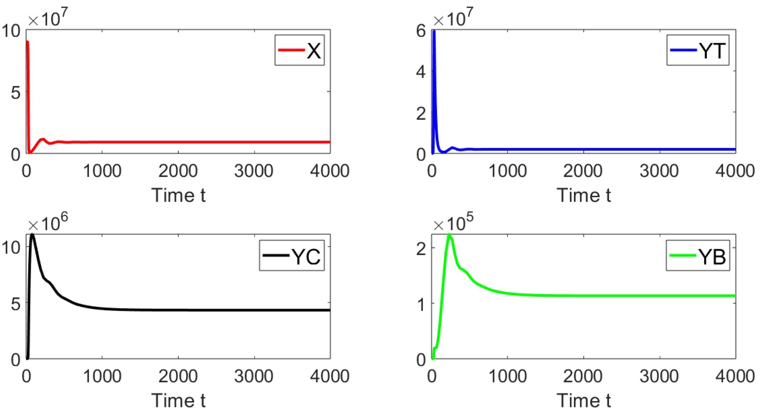
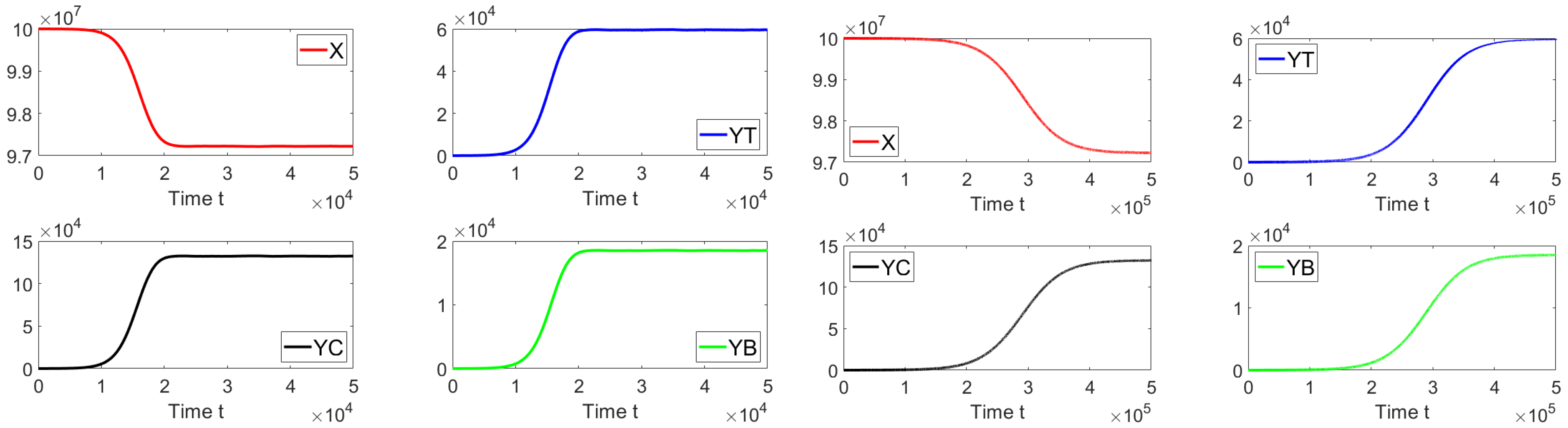
7.2. In Silico Simulations for the Scenarios for ${\mathcal{R}}_0>1$

Now, we deal with in silico simulations where the basic reproduction number ${\mathcal{R}}_0>1$ with a discrete-time delay $\tau$. Figure 7 shows the dynamics of the different sub-populations related to model (19). We take an initial condition that is relatively close to the disease-free equilibrium point or far from the endemic equilibrium point. On the left-hand side we can see that for a discrete time delay of $\tau =1$ the system approaches the endemic equilibrium point. On the right-hand side, the discrete time delay is $\tau =1000$ and the system also approaches the same endemic equilibrium point. 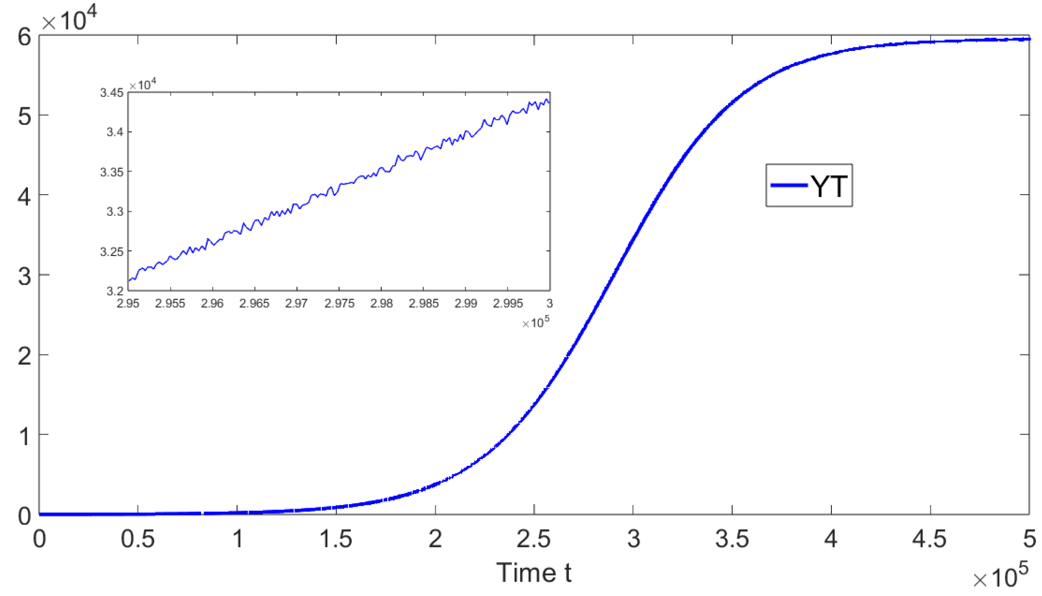These results are in good agreement with the previous theoretical results and also suggest the global stability of the endemic equilibrium point if ${\mathcal{R}}_0>1$. In addition, in Figure 8, the oscillations of the tachyzoite-infected cells sub-population related to model (19) can be seen.

8. Conclusions

We have looked into two mathematical models built on ordinary differential equations for the dynamics of within-host toxoplasmosis and related to the model presented in [3]. These mathematical models include healthy cells, tachyzoite-infected cells, early-stage-bradyzoite-containing cells and encysted-bradyzoite-containing cells. We modified the model in order to take into account for the absence of the immune system’s effector cells. We studied two within-host mathematical models. The first model is based on ordinary differential equations and the second one includes a discrete time delay. The discrete time delay is introduced so that once there is a contact between a healthy cell and a free tachyzoite, the healthy cell does not instantaneously become a tachyzoite-infected cell that can produce free tachyzoites. In addition, this cell cannot become an early-stage-bradyzoite-containing cell right away. Therefore, from a biological point of view, the introduction of time delays makes the model more realistic at the expense of being more complex. The study of the within-host model can be extended in many ways. For instance, additional time delays can be included since there are other within-host biological processes that have delays. However, the introduction of additional time delays would make the mathematical analysis more difficult. Another aspect that can be studied further is the whole within-host model considering the free parasites and carefully taking into account the different time scales.

We initially identified the models’ steady states or equilibrium points and, thereafter, we computed the basic reproduction number ${\mathcal{R}}_0$. Two equilibrium points exist in both models: the first is the disease-free equilibrium point and the second is the endemic equilibrium point. We found that the initial quantity of uninfected cells $X_0$ has an impact on the basic reproduction number ${\mathcal{R}}_0$. This threshold parameter also depends on the contact rate between tachyzoites and uninfected cells ${\beta }_T$, the contact rate between encysted bradyzoite and the uninfected cells ${\beta }_B$, the conversion rate from tachyzoites to bradyzoites $r_T$, and the death rate of the bradyzoites $a_C$ and tachyzoite-infected cells $a_T$.

We investigated the local and global stability of the two equilibrium points for the within-host model based on ordinary differential equations. A Lyapunov function is used to demonstrate the global stability of the endemic point, whereas the comparison approach is used to demonstrate the global stability of the disease-free equilibrium point. We performed numerical simulations to validate our analytical findings. The numerical results supported the theoretical stability analysis.

We also examined the global stability of the disease-free equilibrium point for the within-host model based on delay differential equations. We demonstrated that the disease-free equilibrium point cannot lose stability regardless of the value of the time delay when ${\mathcal{R}}_0<1$. From a biological viewpoint, we can conclude that the time discrete delay does not affect the long-term dynamics. We performed numerical simulations to validate our analytical findings. In addition, we proved that the endemic equilibrium point is globally stable if ${\mathcal{R}}_0>1$ and we performed numerical simulations that support the global stability of the endemic equilibrium point. In summary, we have seen that this threshold parameter is crucial for the dynamics of within-host toxoplasmosis. The sensitivity analysis revealed that the contact rate between tachyzoites and uninfected cells is very important for the dynamics, and that drugs can focus on diminishing the value of this parameter or the process associated with it. Future works can include additional time delays.

References

1. Hill, D.E.; Dubey, J.P. Toxoplasma gondii. In Foodborne Parasites; Springer: Cham, Switzerland, 2018; pp. 119–138. [Google Scholar]
2. Tenter, A.M.; Heckeroth, A.R.; Weiss, L.M. Toxoplasma gondii: From animals to humans. Int. J. Parasitol. 2000, 30, 1217–1258. [Google Scholar] [CrossRef] [PubMed]
3. Sullivan, A.; Agusto, F.; Bewick, S.; Su, C.; Lenhart, S.; Zhao, X. A mathematical model for within-host Toxoplasma gondii invasion dynamics. Math. Biosci. Eng. 2012, 9, 647. [Google Scholar]
4. Baatz, H.; Mirshahi, A.; Puchta, J.; Gümbel, H.; Hattenbach, L.O. Reactivation of toxoplasma retinochoroiditis under atovaquone therapy in an immunocompetent patient. Ocul. Immunol. Inflamm. 2006, 14, 185–187. [Google Scholar] [CrossRef] [PubMed]
5. Dannemann, B.; McCutchan, J.A.; Israelski, D.; Antoniskis, D.; Leport, C.; Luft, B.; Nussbaum, J.; Clumeck, N.; Morlat, P.; Chiu, J.; et al. Treatment of toxoplasmic encephalitis in patients with AIDS: A randomized trial comparing pyrimethamine plus clindamycin to pyrimethamine plus sulfadiazine. Ann. Intern. Med. 1992, 116, 33–43. [Google Scholar] [CrossRef] [PubMed]
6. Aspinall, T.V.; Joynson, D.H.; Guy, E.; Hyde, J.E.; Sims, P.F. The molecular basis of sulfonamide resistance in Toxoplasma gondii and implications for the clinical management of toxoplasmosis. J. Infect. Dis. 2002, 185, 1637–1643. [Google Scholar] [CrossRef] [PubMed]
7. Dubey, J.P. Toxoplasmosis–a waterborne zoonosis. Vet. Parasitol. 2004, 126, 57–72. [Google Scholar] [CrossRef]
8. English, E.D.; Striepen, B. The cat is out of the bag: How parasites know their hosts. PLoS Biol. 2019, 17, e3000446. [Google Scholar] [CrossRef]
9. Innes, E. A brief history and overview of Toxoplasma gondii. Zoonoses Public Health 2010, 57, 1–7. [Google Scholar] [CrossRef]
10. Petersen, E.; Dubey, J. Biology of toxoplasmosis. Toxoplasmosis: A Comprehensive Clinical Guide; Cambrigde University Press: Cambrigde, UK, 2001; pp. 1–42. [Google Scholar]
11. Dubey, J.; Lindsay, D.S. Neosporosis, toxoplasmosis, and sarcocystosis in ruminants. Vet. Clin. Food Anim. Pract. 2006, 22, 645–671. [Google Scholar] [CrossRef]
12. Skariah, S.; McIntyre, M.K.; Mordue, D.G. Toxoplasma gondii: Determinants of tachyzoite to bradyzoite conversion. Parasitol. Res. 2010, 107, 253–260. [Google Scholar] [CrossRef]
13. Conrad, P.; Miller, M.; Kreuder, C.; James, E.; Mazet, J.; Dabritz, H.; Jessup, D.; Gulland, F.; Grigg, M. Transmission of Toxoplasma: Clues from the study of sea otters as sentinels of Toxoplasma gondii flow into the marine environment. Int. J. Parasitol. 2005, 35, 1155–1168. [Google Scholar] [CrossRef] [PubMed]
14. Dubey, J. Unexpected oocyst shedding by cats fed Toxoplasma gondii tachyzoites: In vivo stage conversion and strain variation. Vet. Parasitol. 2005, 133, 289–298. [Google Scholar] [CrossRef] [PubMed]
15. Dubey, J.P.; Beattie, C. Toxoplasmosis of Animals and Man; CRC Press, Inc.: Boca Raton, FL, USA, 1988. [Google Scholar]
16. Blader, I.J.; Saeij, J.P. Communication between Toxoplasma gondii and its host: Impact on parasite growth, development, immune evasion, and virulence. Apmis 2009, 117, 458–476. [Google Scholar] [CrossRef] [PubMed]
17. Arenas, A.J.; González-Parra, G.; Micó, R.J.V. Modeling toxoplasmosis spread in cat populations under vaccination. Theor. Popul. Biol. 2010, 77, 227–237. [Google Scholar] [CrossRef]
18. Deng, H.; Cummins, R.; Schares, G.; Trevisan, C.; Enemark, H.; Waap, H.; Srbljanovic, J.; Djurkovic-Djakovic, O.; Pires, S.M.; van der Giessen, J.W.; et al. Mathematical modelling of Toxoplasma gondii transmission: A systematic review. Food Waterborne Parasitol. 2021, 22, e00102. [Google Scholar] [CrossRef]
19. Ferreira, J.D.; Echeverry, L.M.; Rincon, C.A.P. Stability and bifurcation in epidemic models describing the transmission of toxoplasmosis in human and cat populations. Math. Methods Appl. Sci. 2017, 40, 5575–5592. [Google Scholar] [CrossRef]
20. González-Parra, G.C.; Arenas, A.J.; Aranda, D.F.; Villanueva, R.J.; Jódar, L. Dynamics of a model of Toxoplasmosis disease in human and cat populations. Comput. Math. Appl. 2009, 57, 1692–1700. [Google Scholar] [CrossRef]
21. González-Parra, G.; Arenas, A.J.; Chen-Charpentier, B.; Sultana, S. Mathematical modeling of toxoplasmosis with multiple hosts, vertical transmission and cat vaccination. Comput. Appl. Math. 2023, 42, 88. [Google Scholar] [CrossRef]
22. Lélu, M.; Langlais, M.; Poulle, M.L.; Gilot-Fromont, E. Transmission dynamics of Toxoplasma gondii along an urban–rural gradient. Theor. Popul. Biol. 2010, 78, 139–147. [Google Scholar] [CrossRef]
23. Sultana, S.; González-Parra, G.; Arenas, A.J. A Generalized Mathematical Model of Toxoplasmosis with an Intermediate Host and the Definitive Cat Host. Mathematics 2023, 11, 1642. [Google Scholar] [CrossRef]
24. Turner, M.; Lenhart, S.; Rosenthal, B.; Zhao, X. Modeling effective transmission pathways and control of the world’s most successful parasite. Theor. Popul. Biol. 2013, 86, 50–61. [Google Scholar] [CrossRef] [PubMed]
25. Ogunmiloro, O.M. Mathematical Modeling of the Coinfection Dynamics of Malaria-Toxoplasmosis in the Tropics. Biom. Lett. 2019, 56, 139–163. [Google Scholar] [CrossRef]
26. Sultana, S.; González-Parra, G.; Arenas, A.J. Dynamics of toxoplasmosis in the cat’s population with an exposed stage and a time delay. Math. Biosci. Eng. 2022, 19, 12655–12676. [Google Scholar] [CrossRef]
27. Sultana, S.; González-Parra, G.; Arenas, A.J. Mathematical modeling of toxoplasmosis considering a time delay in the infectivity of oocysts. Math. Biosci. Eng. 2022, 19, 12655–12676. [Google Scholar] [CrossRef] [PubMed]
28. Wormser, G.P.; Pourbohloul, B. Modeling Infectious Diseases in Humans and Animals By Matthew James Keeling and Pejman Rohani Princeton, NJ: Princeton University Press, 2008. 408 pp., Illustrated. $65.00 (hardcover). Clin. Infect. Dis. 2008, 47, 864–865. [Google Scholar]
29. Murray, J.D. Mathematical Biology: I. An Introduction; Interdisciplinary Applied Mathematics; Springer: Berlin/Heidelberg, Germany, 2002; Volume 17. [Google Scholar]
30. Wodarz, D. Killer Cell Dynamics: Mathematical and Computational Approaches to Immunology; Springer: Berlin/Heidelberg, Germany, 2007. [Google Scholar]
31. Cerutti, A.; Blanchard, N.; Besteiro, S. The bradyzoite: A key developmental stage for the persistence and pathogenesis of toxoplasmosis. Pathogens 2020, 9, 234. [Google Scholar] [CrossRef]
32. van den Driessche, P.; Watmough, J. Reproduction numbers and sub-threshold endemic equilibria for compartmental models of disease transmission. Math. Biosci. 2002, 180, 29–48. [Google Scholar] [CrossRef]
33. Routh, E.J. A Treatise on the Stability of a Given State of Motion: Particularly Steady Motion. Being the Essay to Which the Adams Prize Was Adjudged in 1877, in the University of Cambridge; Macmillan and Company: London, UK, 1877. [Google Scholar]
34. Korobeinikov, A. Lyapunov functions and global stability for SIR and SIRS epidemiological models with non-linear transmission. Bull. Math. Biol. 2006, 68, 615–626. [Google Scholar] [CrossRef]
35. Korobeinikov, A.; Wake, G.C. Lyapunov functions and global stability for SIR, SIRS, and SIS epidemiological models. Appl. Math. Lett. 2002, 15, 955–960. [Google Scholar] [CrossRef]
36. Vargas-De-León, C. On the global stability of SIS, SIR and SIRS epidemic models with standard incidence. Chaos Solitons Fractals 2011, 44, 1106–1110. [Google Scholar] [CrossRef]
37. Castillo-Garsow, C.W.; Castillo-Chavez, C. A tour of the basic reproductive number and the next generation of researchers. In An Introduction to Undergraduate Research in Computational and Mathematical Biology; Springer: Berlin/Heidelberg, Germany, 2020; pp. 87–124. [Google Scholar]
38. Chitnis, N.; Hyman, J.M.; Cushing, J.M. Determining important parameters in the spread of malaria through the sensitivity analysis of a mathematical model. Bull. Math. Biol. 2008, 70, 1272–1296. [Google Scholar] [CrossRef] [PubMed]
39. Florian, F.; Vermiglio, R. PC-based sensitivity analysis of the basic reproduction number of population and epidemic models. In Current Trends in Dynamical Systems in Biology and Natural Sciences; Springer: Berlin/Heidelberg, Germany, 2020; pp. 205–222. [Google Scholar]
40. Samsuzzoha, M.; Singh, M.; Lucy, D. Uncertainty and sensitivity analysis of the basic reproduction number of a vaccinated epidemic model of influenza. Appl. Math. Model. 2013, 37, 903–915. [Google Scholar] [CrossRef]
41. Vermiglio, R.; Zamolo, A. Sensitivity analysis for stability of uncertain delay differential equations using polynomial chaos expansions. In Accounting for Constraints in Delay Systems; Springer: Berlin/Heidelberg, Germany, 2022; pp. 151–173. [Google Scholar]
42. Kajiwara, T.; Sasaki, T.; Takeuchi, Y. Construction of Lyapunov functionals for delay differential equations in virology and epidemiology. Nonlinear Anal. Real World Appl. 2012, 13, 1802–1826. [Google Scholar] [CrossRef]
43. McCluskey, C.C. Using Lyapunov functions to construct Lyapunov functionals for delay differential equations. SIAM J. Appl. Dyn. Syst. 2015, 14, 1–24. [Google Scholar] [CrossRef]
Figure 1. A diagram illustrating the model (3) for within-host invasion dynamics.
Mathematics 11 04469 g001
Figure 2. Dynamics of the different sub-populations when β T = 5 × 10 10 , β B = 5 × 10 11 , and R 0 0.9428 . The initial condition is X ( 0 ) = 0.9 × 10 8 , Y T ( 0 ) = 10 , Y C ( 0 ) = 10 and Y B ( 0 ) = 10 .
Mathematics 11 04469 g002
Figure 3. Dynamics of the different sub-populations when β T = 5 × 10 10 , β B = 5 × 10 11 , and R 0 0.9428 . The initial condition is X ( 0 ) = 10 6 , Y T ( 0 ) = 2 × 10 6 , Y C ( 0 ) = 4 × 10 6 and Y B ( 0 ) = 1 × 10 5 . This initial condition is very far away from the disease-free equilibrium point.
Mathematics 11 04469 g003
Figure 4. Dynamics of the different sub-populations when β T = 7 × 10 9 , β B = 6 × 10 11 , and R 0 11.00571 . The initial condition is X ( 0 ) = 0.9 × 10 8 , Y T ( 0 ) = 10 , Y C ( 0 ) = 10 , and Y B ( 0 ) = 10 . This initial condition is close to the disease-free equilibrium point.
Mathematics 11 04469 g004
Figure 5. Sensitivity plot of the basic reproduction number R 0 related to the parameter a C (death rate of encysted-bradyzoite-infected cells).
Mathematics 11 04469 g005
Figure 6. Dynamics of the different sub-populations when β T = 6 × 10 10 , β B = 1 × 10 11 and R 0 0.96 . The initial condition is X ( 0 ) = 1 × 10 8 , Y T ( 0 ) = 1 × 10 5 , Y C ( 0 ) = 1 × 10 5 , and Y B ( 0 ) = 1 × 10 5 . The time delays are τ = 1 (left) and τ = 1000 (right).
Mathematics 11 04469 g006
Figure 7. Dynamics of the different sub-populations when β T = 6 × 10 10 , β B = 3 × 10 11 and R 0 1.02 . The initial condition is X ( 0 ) = 1 × 10 8 , Y T ( 0 ) = 10 , Y C ( 0 ) = 10 , and Y B ( 0 ) = 10 . The time delays are τ = 1 (left) and τ = 1000 (right).
Mathematics 11 04469 g007
Figure 8. Dynamics of the tachyzoite-infected cells ( Y T ) sub-population when β T = 6 × 10 10 , β B = 3 × 10 11 and R 0 1.02 . The initial condition is X ( 0 ) = 1 × 10 8 , Y T ( 0 ) = 10 , Y C ( 0 ) = 10 , and Y B ( 0 ) = 10 . The time delay is τ = 1000 .
Mathematics 11 04469 g008