An Integrated Group Decision-Making Framework for the Evaluation of Artificial Intelligence Cloud Platforms Based on Fractional Fuzzy Sets

Abstract

Due to the rapid development of machine learning and artificial intelligence (AI), the analysis of AI cloud platforms is now a key area of research. Assessing the wide range of frameworks available and choosing the ideal AI cloud providers that may accommodate the demands and resources of a company is mandatory. There are several options, all having their own benefits and limitations. The evaluation of artificial intelligence cloud platforms is a multiple criteria group decision-making (MCGDM) process. This article establishes a collection of Einstein geometric aggregation operators (AoPs) and a novel Fractional Fuzzy VIKOR and Fractional Fuzzy Extended TOPSIS based on the entropy weight of criteria in fractional fuzzy sets (FFSs) for this scenario. The FFSs provide an evaluation circumstance containing more information, which makes the final decision-making results more accurate. Finally, this framework is then implemented in a computational case study for the evaluation of artificial intelligence cloud platforms and comparison of this model with other existing approaches, such as the extended GRA approach, to check the consistency and accuracy of the proposed technique. The most optimal artificial intelligence cloud platform is ${\mathfrak{I}}_1$

1. Introduction

Machine learning (ML) may be highly suitable for cloud computing applications. Cloud services allow for fast deployment. Spin-down, shutdown, and activation of large-scale computing collections with zero downtime, with information never leaving the servers or IT system of enterprises. Cloud services are adaptable as enterprises develop. Approaches involving artificial intelligence (AI) are especially beneficial in this context. In particular, certain assignments may demand that AI models be trained on hundreds of terabytes of organized information. Consequently, developers do not need to start tasks from the beginning. These characteristics guarantee that AI development is effective, obtainable, and comprehensible. Cloud AI platforms deliver an entirely novel environment for business enterprises that want to explore AI but may not know where to start [1,2,3,4]. Due to the rising use of AI technologies, analysis of cloud platforms that offer AI services is becoming more and more crucial. Yet, existing evaluation techniques frequently fail to identify ambiguity and uncertainty related to decision-making in this circumstance. The problems present in the analysis of AI cloud service platforms were recently investigated utilizing the multi-criteria group decision-making (MCGDM) method [5,6,7]. Therefore, many theories were developed to handle the uncertainty and impreciseness in such scenarios. First of all, L.A Zadeh [8] in 1965 developed the notion of a new set called fuzzy set (FS) having one positive degree of membership (DM) and that DM belongs to the close interval [0, 1]. The FS has failed to illustrate the uncertainty of an object because there is no analysis of the non-membership degree. To cover this drawback, Attanassov [9,10] introduced the new notion of the intuitionistic fuzzy set (IFS) having two degrees: one is the positive degree of membership (DM), and the other is called the degree of negative non-membership (DNM) with the condition that the sum of these two degrees is always in the domain of zero and one. The IFS is of great importance in decision-making (DM) and is supposed to be the most powerful tool for dealing with uncertainties in MCDM scenarios. However, after some time, there are many cases where the accumulation of DM and DNM exceeds one, which violates the basic property of IFS. To handle these limitations of IFS, Yager [11,12] introduced the phrase concept of a new set called Pythagorean fuzzy set (PyFS), also with two degrees: one is the positive DM, and the other is the negative DNM with the condition that the accumulation of the squares of DM and DNM always pertain to the close interval [0, 1]. PyFS is more widely used in decision-making (DM) issues than IFS and FS. PyFS restricts the decision experts in many real-world problems. To deal with these limitations, more detailed algorithms were needed. After that, Yager [13] broadened the concept of PyFS and established the new notion of a set called q-rung orthopair fuzzy set (𝓺-ROFS) having also two degrees; one is DM and the other is DNM with the condition that the sum of the ${\mathcal{q}}^{\mathrm{t}\mathrm{h}}$ $(\mathcal{q}\in \mathbb{Z})$ power of DM and DNM pertains to the close interval zero and one. It is the generalized form of PyFS, IFS, and FS. After the development of 𝓺-ROFS many scholars researched and solved many real-life decision-making (MD) problems which was not solved by other extensions of FS. However, 𝓺-ROFS also has some limitations because its domain has no analysis about the fractional numbers (FNs). To solve this problem, Abdullah et al. [14] extended the domain of 𝓺-ROFS to fractional numbers (FNs) and developed the notion of a new set called fractional fuzzy set (FFS), which is also a two-degree system, but here one degree is called DM, and the other is DNM with the condition that 0 $\le {\mathsf{\eta }}_{\mathsf{F}}^{\mathbb{f}}$ +${\upsilon }_{\mathsf{F}}^{\mathbb{f}}\le$ 1 where ($\mathbb{f}=\mathbb{p}/\mathbb{q}$) is fractional number (FN). FFS generalized all the extensions of FSs.

From the above literature review, we concluded that no study has been conducted on the fractional fuzzy set (FFS). The FFS is the extension of FS, IFS, PyFS, and q-ROFS. So, we define the Einstein sum and product in an FFS environment, and on the basis of these Einstein operations, we define Einstein operational laws and their application to real-world decision-making problems.

1.1. Related Studies

The role of aggregation operators (AoPs) is very advantageous in MCDM problems. Aggregation operators are used to collect (aggregate) the expert knowledge that exceeds the knowledge of individual experts. Now, there are some Einstein geometric aggregation operators (AoPs) in the literature review, which are based on different extensions of fuzzy sets (FS). Some of them are reviewed as follows. Zhao et al. [15] defined a collection of Einstein AoPs and also applied them to real-life situations in an IF environment. Abdullah et al. [16] and Mahmood et al. [17] discussed a series of Einstein AoPs and their application to decision-making for PyFS information. Zulqarnain et al. [18] and Wu et al. [19] reviewed a group of Einstein geometric AoPs for q-ROF information and also applied them to a decision-making system.

Consequently, keeping in mind the significance and application of the aforementioned aggregation operators in our proposed study, we broadened the already existing operators and introduced the notion of fractional fuzzy Einstein geometric aggregation operators (AoPs) in an FFS environment.

Methods are the specific tools and procedures you use to collect and analyze data and find the best optimal alternative. Different techniques are used to help us in various group decision-making problems. Here, we discussed some methods as follows. Vikram et al. [20] discussed the steps of extended TOPSIS methods applied to decision-making problems in an IF environment. Lue et al. [21] also discussed the main points of the extended TOPSIS method in an IF environment. After that, Zhang and Zeshui [22] discussed the steps of the extended TOPSIS method and its applications to decision-making problems in a PyFS environment. Fatih et al. [23] also discussed the steps of the extended TOPSIS method and applied it to a real-life (risk analysis) decision-making scenario of PyFS information. Recently, Ravinder [24] discussed the steps of the extended TOPSIS method and its application to many real-world complex problems on PyFS information. Mehmet et al. [25] extended the extended TOPSIS method to a q-ROFS environment and its application to multi-criteria decision-making problems. Furthermore, Jakub et al. [26] discussed the steps of the VIKOR method in an IF environment. Pratibha [27] highlighted the steps of the VIKOR method in a PyFS environment and applied it to decision-making problems (DMPs). Further, many scholars [28,29,30] analyzed the VIKOR approach for different advancements of FSs.

Based on the above literature review, we conclude that there is no extensive utilization of the extended TOPSIS method and VIKOR method applied to FFS information.

1.2. Motivation of This Study

Based on the above literature review, the authors reach the result that there is no remarkable study implemented on FFS information. The motivation supporting this technique is to present a more detailed and comprehensive analysis of AI cloud platforms by including a variety of parameters and implementing along the vagueness present in personal assessments. Using FFSs, the motivation of the developed study is outlined as follows;

• To define new Einstein operational laws in an FFS environment.
• On the basis of these operational laws, define a new set of Einstein geometric aggregation operators (AoPs) in the same environment.
• To develop a new approach to the extended TOPSIS method and VIKOR method in an FFS environment.
• To verify and apply the proposed method to a real-life decision-making issue, as discussed below.

1.3. Contribution of This Study

From the above overall discussion, the authors conclude that there is no utilization of FFS information in any decision support system. So, we proposed some studies on FFS. As demonstrated by the earlier discussion of the literature studies that are currently available, a qualitative study analyzing the AICP using the VIKOR approach and the extended TOPSIS approach under FFSs has still not been conducted. Therefore, the VIKOR approach and the extended TOPSIS technique under FFSs are proposed to analyze the AICP MCGDM. The main contributions of this study are outlined as follows:

• We defined new Einstein operational laws in an FFS environment.
• On the basis of these operational laws, we defined a new Einstein geometric aggregation operator (AoPs) in an FFS environment.
• The FF–VIKOR technique and FF-Extended TOPSIS approach were formulated for MCGDM issues in an FFS environment.
• We verified our proposed method with a real-life decision-making issue for the evaluation of artificial intelligence cloud platforms.

The structure of the study is outlined as follows. We write the introduction in the Section 1. In Section 2, the fundamental knowledge related to FS is discussed. The Einstein norms and operational laws are reviewed, and on the basis of these laws, we propose Einstein geometric aggregation operators in Section 3. The Methodology-I of the extended TOPSIS method is analyzed in Section 4. The Methodology of the VIKOR method is discussed in Section 5. A real-life case study was discussed in Section 6. The numerical results of the proposed VIKOR method are in Section 7. The numerical results of the proposed extended TOPSIS method are discussed in Section 8. Comparative analysis and discussion are examined in Section 9. In Section 10, we end with the conclusion.

2. Fundamental Knowledge

Let $\mathbb{Z}\ne \varphi$ be a non-empty set. An FS 𝔒 can be described in the form of a mathematical expression, 𝔒 =$\left\{〈\mathbb{z},{\tilde{\mathsf{\eta }}}_{\mathfrak{O}}\left(\mathbb{z}\right)〉|\mathbb{z}\in \mathbb{Z}\right\}$, where ${\mathsf{\eta }}_{\mathcal{B}}$ is a mapping $\mathbb{Z}:{\mathsf{\eta }}_{\mathcal{B}}\to$ $\left[0, 1\right]$ and for each $\mathbb{z}\in \mathbb{Z}$, ${\mathsf{\eta }}_{\mathcal{B}}\left(\mathbb{z}\right)$ is known as the grade of membership of $\mathbb{z}$ in $\mathbb{Z}$. An IFS $\mathrm{Ῐ}$ can be defined as equation $\mathrm{Ῐ}=\left\{〈\mathbb{z},{\tilde{\mathsf{\eta }}}_{\mathrm{Ῐ}}\left(\mathbb{z}\right),{\tilde{\upsilon }}_{\mathrm{Ῐ}}\left(\mathbb{z}\right)〉|\mathbb{z}\in \mathbb{Z}\right\}$, where ${\tilde{\mathsf{\eta }}}_{\mathrm{Ῐ}}\left(\mathbb{z}\right)$ and ${\tilde{\upsilon }}_{\mathrm{Ῐ}}\left(\mathbb{z}\right)$ are mapping from $\mathbb{Z}$ to $[0, 1]$ with the condition $0 \le {\tilde{\mathsf{\eta }}}_{\mathrm{Ῐ}}\left(\mathbb{z}\right)+{\tilde{\upsilon }}_{\mathrm{Ῐ}}\left(\mathbb{z}\right)\le 1$ for every $\mathbb{z}$ in $\mathbb{Z}$. The PFS P can be defined as P $=\left\{〈\mathbb{z},{\tilde{\mathsf{\eta }}}_{\mathrm{P}}\left(\mathbb{z}\right),{\tilde{\upsilon }}_{\mathrm{P}}\left(\mathbb{z}\right)〉|\mathbb{z}\in \mathbb{Z}\right\}$, where ${\tilde{\mathsf{\eta }}}_{\mathrm{P}}\left(\mathbb{z}\right),{\tilde{\upsilon }}_{\mathrm{P}}\left(\mathbb{z}\right)$:$\mathbb{Z}\to$ [0, 1] with the condition that 0$\le {{\tilde{\mathsf{\eta }}}_{\mathrm{P}}}^2\left(\mathbb{z}\right)+{{\tilde{\upsilon }}_{\mathrm{P}}}^2\left(\mathbb{z}\right)\le$1 for all $\mathbb{z}\in \mathbb{Z},$ and they represent the degree of MD and DNM of an object $\mathbb{z}\in \mathbb{Z}$ to the set P. Let ${\pi }_{\mathrm{P}}$($\mathbb{z}$) = $\sqrt{1-{\tilde{\mathsf{\eta }}}_{\mathrm{P}}\left(\mathbb{z}\right)-{\tilde{\upsilon }}_{\mathrm{P}}\left(\mathbb{z}\right)}$ is denotes indeterminacy membership degree of $\mathbb{z}$. Let $\mathbb{Z}\ne \varphi$ be a non-empty set. The 𝓺-ROFS $\mathfrak{Q}$ can be defined as, $\mathfrak{Q}=\left\{〈\mathbb{z},{\tilde{\mathsf{\eta }}}_{\mathfrak{Q}}\left(\mathbb{z}\right),{\tilde{\upsilon }}_{\mathfrak{Q}}\left(\mathbb{z}\right)〉,0\le {{\tilde{\mathsf{\eta }}}_{\mathfrak{Q}}}^{\mathcal{q}}\left(\mathbb{z}\right)+{{\tilde{\upsilon }}_{\mathfrak{Q}}}^{\mathcal{q}}\left(\mathbb{z}\right)\le 1|\mathbb{z}\in \mathbb{Z}\right\}$, where ${\tilde{\mathsf{\eta }}}_{\mathrm{P}}\left(\mathbb{z}\right),{\tilde{\upsilon }}_{\mathrm{P}}\left(\mathbb{z}\right)$ are the function of membership and non-membership and always belong to [0, 1] and ${\mathsf{\Omega }}_{\mathfrak{Q}}\left(\mathbb{z}\right)=\sqrt[\mathcal{q}]{1-{{\tilde{\mathsf{\eta }}}_{\mathfrak{Q}}}^{\mathcal{q}}\left(\mathbb{z}\right)-{{\tilde{\upsilon }}_{\mathfrak{Q}}}^{\mathcal{q}}\left(\mathbb{z}\right)}$ are the degree of indeterminacy. The FFS is a F mathematical object of the form F $=\left\{〈\mathbb{z},{\tilde{\mathsf{\eta }}}_{\mathsf{F}}\left(\mathbb{z}\right),{\tilde{\upsilon }}_{\mathsf{F}}\left(\mathbb{z}\right)〉,0\le {{\tilde{\mathsf{\eta }}}_{\mathsf{F}}}^{\mathbb{f}}\left(\mathbb{z}\right)+{{\tilde{\upsilon }}_{\mathsf{F}}}^{\mathbb{f}}\left(\mathbb{z}\right)\le 1|\mathbb{z}\in \mathbb{Z}\right\}$ where ($\mathbb{f}=\mathbb{p}/\mathbb{q}$) and ${\tilde{\mathsf{\eta }}}_{\mathsf{F}}$:$\mathbb{X}\to \left[\mathrm{0,1}\right]$ and ${\tilde{\upsilon }}_{\mathsf{F}}$:$\mathbb{X}\to \left[\mathrm{0,1}\right]$ are the membership and NM mappings with the condition that 0 $\le {\mathsf{\eta }}_{\mathsf{F}}^{\mathbb{f}}$ +${\upsilon }_{\mathsf{F}}^{\mathbb{f}}\le$1 for all $\mathbb{z}\in \mathbb{Z}$. In addition, ${\mathsf{\Omega }}_{\mathsf{F}}\left(\mathbb{z}\right)=\sqrt[\mathbb{f}]{1-{{\tilde{\mathsf{\eta }}}_{\mathsf{F}}}^{\mathbb{f}}\left(\mathbb{z}\right)-{{\tilde{\upsilon }}_v}^{\mathbb{f}}\left(\mathbb{z}\right)}$ denote the indeterminacy MD of $\mathbb{z}\in \mathbb{Z}.$

From the above equations, it can be determined that among q-ROFS, IFS, and PFS, FFS is the most popular type with the condition that 0 $\le {\mathsf{\eta }}_{\mathsf{F}}^{\mathbb{f}}$ +${\upsilon }_{\mathsf{F}}^{\mathbb{f}}\le$1, where $(\mathbb{f}=\mathbb{p}/\mathbb{q})$, when $\mathbb{p}$ and $\mathbb{q}$ take distinct numbers, we obtain distinct FSs.

Case 1.

If $(\mathbb{f}=\frac{\mathbb{p}}{\mathbb{q}}\ge 1,\mathbb{p}=\mathbb{q}=1)$, then the FF set becomes the IF set.

$\mathrm{Ῐ}=\left\{〈\mathbb{z},{\tilde{\mathsf{\eta }}}_{\mathrm{Ῐ}}\left(\mathbb{z}\right),{\tilde{\upsilon }}_{\mathrm{Ῐ}}\left(\mathbb{z}\right)〉|\mathbb{z}\in \mathbb{Z}\right\}$ with subject $0 \le {\tilde{\mathsf{\eta }}}_{\mathrm{Ῐ}}\left(\mathbb{z}\right)+{\tilde{\upsilon }}_{\mathrm{Ῐ}}\left(\mathbb{z}\right)\le 1$ for all $\mathbb{z}\in \mathbb{Z}$.

Case 2.

If $(\mathbb{f}=\frac{\mathbb{p}}{\mathbb{q}}\ge 1,\mathbb{p}=2\mathbb{q})$, then the FF set becomes the PyFS set.

P $=\left\{〈\mathbb{z},{\tilde{\mathsf{\eta }}}_{\mathrm{P}}\left(\mathbb{z}\right),{\tilde{\upsilon }}_{\mathrm{P}}\left(\mathbb{z}\right)〉|\mathbb{z}\in \mathbb{Z}\right\}$ with the condition that 0$\le {{\tilde{\mathsf{\eta }}}_{\mathrm{P}}}^2\left(\mathbb{z}\right)+{{\tilde{\upsilon }}_{\mathrm{P}}}^2\left(\mathbb{z}\right)\le$1 for all $\mathbb{z}\in \mathbb{Z}$.

Case 3.

If $(\mathbb{f}=\frac{\mathbb{p}}{\mathbb{q}}\ge 1, \mathbb{p}=3,\mathbb{q}=1)$, then FFS reduces to Farmatean fuzzy set.

$\mathfrak{Q}=\left\{〈\mathbb{z},{\tilde{\mathsf{\eta }}}_{\mathfrak{Q}}\left(\mathbb{z}\right),{\tilde{\upsilon }}_{\mathfrak{Q}}\left(\mathbb{z}\right)〉,0\le {{\tilde{\mathsf{\eta }}}_{\mathfrak{Q}}}^3\left(\mathbb{z}\right)+{{\tilde{\upsilon }}_{\mathfrak{Q}}}^3\left(\mathbb{z}\right)\le 1|\mathbb{z}\in \mathbb{Z}\right\}$ for all $\mathbb{z}\in \mathbb{Z}$.

Case 4.

If $(\mathbb{f}=\frac{\mathbb{p}}{\mathbb{q}}\ge 1, \mathbb{p}\ge 3,\mathbb{q}=1)$, then FFS reduces to 𝓺-ROFS.

$\mathfrak{Q}=\left\{〈\mathbb{z},{\tilde{\mathsf{\eta }}}_{\mathfrak{Q}}\left(\mathbb{z}\right),{\tilde{\upsilon }}_{\mathfrak{Q}}\left(\mathbb{z}\right)〉,0\le {{\tilde{\mathsf{\eta }}}_{\mathfrak{Q}}}^{\mathcal{q}}\left(\mathbb{z}\right)+{{\tilde{\upsilon }}_{\mathfrak{Q}}}^{\mathcal{q}}\left(\mathbb{z}\right)\le 1|\mathbb{z}\in \mathbb{Z}\right\}$ for all $\mathbb{z}\in \mathbb{Z}$.

Let $\mathfrak{R}$ =$({\tilde{\mathsf{\eta }}}_{\mathfrak{R}},{\tilde{\upsilon }}_{\mathfrak{R}}$) be a FFN. Then, the score function $\mathbb{S}\mathbb{r}\left(\mathfrak{R}\right)$ and accuracy function $\mathbb{A}\mathbb{r}\left(\mathfrak{R}\right)$ can be defined as follow:

$$\mathbb{S}\mathbb{r}\left(\mathfrak{R}\right)={{\tilde{\mathsf{\eta }}}_{\mathfrak{R}}\left(\mathbb{z}\right)}^{\mathbb{f}}-{{\tilde{\upsilon }}_{\mathfrak{R}}\left(\mathbb{z}\right)}^{\mathbb{f}}, \mathrm{where}-1\le \mathbb{S}\mathbb{r}\left(\mathbb{z}\right)\ge 1$$

$$\mathbb{A}\mathbb{r}\left(\mathfrak{R}\right)={{\tilde{\mathsf{\eta }}}_{\mathfrak{R}}\left(\mathbb{z}\right)}^{\mathbb{f}}+{{\tilde{\upsilon }}_{\mathfrak{R}}\left(\mathbb{z}\right)}^{\mathbb{f}}, \mathrm{where} 0\le \mathbb{S}\mathbb{r}\left(\mathbb{z}\right)\ge 1$$

3. Fractional Fuzzy Einstein norms and Aggregation Operators (AoPs)

Let S and T be two fractional fuzzy numbers (FFNs). Then, the Einstein norms are defined as,

$$\mathrm{S}⨂\mathrm{T}=\frac{\mathrm{S}{.}_{\mathsf{ϵ}}\mathrm{T}}{\sqrt[\mathbb{f}]{1+\left(1-{\mathrm{S}}^{\mathbb{f}}\right){.}_{\mathsf{ϵ}}(1-{\mathrm{T}}^{\mathbb{f}})}}$$

(1)

$$\mathrm{S}⨁\mathrm{T}=\sqrt[\mathbb{f}]{\frac{{\mathrm{S}}^{\mathbb{f}}+{\mathrm{T}}^{\mathbb{f}}}{1+{\mathrm{S}}^{\mathbb{f}}.\mathsf{ϵ}{\mathrm{T}}^{\mathbb{f}}}}$$

(2)

3.1. Fractional Fuzzy Einstein Operational Laws

In the current section, first, we introduced the fractional fuzzy Einstein operational laws based on Einstein t-norm and t-conorm in an FFS setting.

$${\mathfrak{R}}_1{⨁}_{\mathsf{ϵ}}{\mathfrak{R}}_2=\left(\sqrt[\mathbb{f}]{\frac{{{\tilde{\mathsf{\eta }}}_1}^{\mathbb{f}}+{{\tilde{\mathsf{\eta }}}_2}^{\mathbb{f}}}{1+{{\tilde{\mathsf{\eta }}}_1}^{\mathbb{f}}{.}_{\mathsf{ϵ}}{{\tilde{\mathsf{\eta }}}_2}^{\mathbb{f}}}},\frac{{\tilde{\upsilon }}_{1{.}_{\mathsf{ϵ}}}{\tilde{\upsilon }}_2}{\sqrt[\mathbb{f}]{1+\left(1-{{\tilde{\upsilon }}_1}^{\mathbb{f}}\right){.}_{\mathsf{ϵ}}(1-{{\tilde{\upsilon }}_2}^{\mathbb{f}})}}\right)$$

(3)

$${\mathfrak{R}}_1{⨂}_{\mathsf{ϵ}}{\mathfrak{R}}_2=\left(\frac{{\mathrm{a}}_1{.}_{\mathsf{ϵ}}{\mathrm{a}}_2}{\sqrt[\mathbb{f}]{1+\left(1-{\tilde{\mathsf{\eta }}}_1^{\mathbb{f}}\right){.}_{\mathsf{ϵ}}\left(1-{\tilde{\mathsf{\eta }}}_2^{\mathbb{f}}\right)}},\sqrt[\mathbb{f}]{\frac{{\tilde{\upsilon }}_1^{\mathbb{f}}{.}_{\mathsf{ϵ}}{\tilde{\upsilon }}_2^{\mathbb{f}}}{1+{\tilde{\upsilon }}_1^{\mathbb{f}}{.}_{\mathsf{ϵ}}{\tilde{\upsilon }}_2^{\mathbb{f}}}}\right)$$

(4)

$$\mathcal{I}{.}_{\mathsf{ϵ}}\mathfrak{R}=\left(\sqrt[\mathbb{f}]{\frac{{\left(1+{\tilde{\mathsf{\eta }}}^{\mathbb{f}}\right)}^{\mathcal{I}}+{\left(1-{\tilde{\mathsf{\eta }}}^{\mathbb{f}}\right)}^{\mathcal{I}}}{{\left(1+{\tilde{\mathsf{\eta }}}^{\mathbb{f}}\right)}^{\mathcal{I}}+{\left(1-{\tilde{\mathsf{\eta }}}^{\mathbb{f}}\right)}^{\mathcal{I}}}},\frac{\sqrt[\mathbb{f}]{2}{\tilde{\upsilon }}^{\mathcal{I}}}{\sqrt[\mathbb{f}]{{\left(2-{\tilde{\upsilon }}^{\mathbb{f}}\right)}^{\mathcal{I}}+{\left({\tilde{\upsilon }}^{\mathbb{f}}\right)}^{\mathcal{I}}}}\right)$$

(5)

$${\mathfrak{R}}^{\mathsf{\gamma }}=\left(\frac{\sqrt[\mathbb{f}]{2}{·}_{\mathsf{ϵ}}{\tilde{\mathsf{\eta }}}^{\mathsf{\gamma }}}{\sqrt[\mathbb{f}]{{\left(2-{\tilde{\mathsf{\eta }}}^{\mathbb{f}}\right)}^{\mathsf{\gamma }}+{\tilde{\mathsf{\eta }}}^{\mathbb{f}\mathsf{\gamma }}}},\sqrt[\mathbb{f}]{\frac{{\left(1+{\tilde{\upsilon }}^{\mathbb{f}}\right)}^{\mathsf{\gamma }}-{\left(1-{\tilde{\upsilon }}^{\mathbb{f}}\right)}^{\mathsf{\gamma }}}{{\left(1+{\tilde{\upsilon }}^{\mathbb{f}}\right)}^{\mathsf{\gamma }}+{\left(1-{\tilde{\upsilon }}^{\mathbb{f}}\right)}^{\mathsf{\gamma }}}}\right)$$

(6)

3.2. Fractional Fuzzy Einstein Geometric Aggregation Operators

Here, we shall develop the fractional fuzzy geometric aggregation operators with the help of Einstein norms and operational laws. Now we discuss one by one as follows:

3.3. Fractional Fuzzy Einstein Weighted Geometric Aggregation Operator (AoP)

Let ${\mathfrak{R}}_{\mathsf{\rho }}=({\tilde{\mathsf{\eta }}}_{{\mathfrak{R}}_{\mathsf{\rho }}},{\tilde{\upsilon }}_{{\mathfrak{R}}_{\mathsf{\rho }}})\left(\mathsf{\rho }=1, 2, 3, \dots n\right)$ be a collection of all fractional fuzzy numbers. Then, the fractional fuzzy Einstein weighted geometric FFEWG aggregation operator can be defined as where ($\mathbb{f}=\mathbb{p}/\mathbb{q}$),

$$\begin{array}{c}{\mathrm{F}\mathrm{F}\mathrm{E}\mathrm{W}\mathrm{G}}_{\mathcal{w}}\left({\mathfrak{R}}_1,{\mathfrak{R}}_2,{\mathfrak{R}}_3,...,{\mathfrak{R}}_{\mathrm{n}}\right)=\hfill \\ \left(\frac{\sqrt[\mathbb{f}]{2\prod _{\mathsf{\rho }=1}^{\mathrm{n}}{\left({{\tilde{\mathsf{\eta }}}_{{\mathfrak{R}}_{\mathsf{\rho }}}}^{\mathbb{f}}\right)}^{{\mathcal{w}}_{\mathsf{\rho }}}}}{\sqrt[\mathbb{f}]{\prod _{\mathsf{\rho }=1}^{\mathrm{n}}{\left(2-{{\tilde{\mathsf{\eta }}}_{{\mathfrak{R}}_{\mathsf{\rho }}}}^{\mathbb{f}}\right)}^{{\mathcal{w}}_{\mathsf{\rho }}}+\prod _{\mathsf{\rho }=1}^{\mathrm{n}}{\left({{\tilde{\mathsf{\eta }}}_{{\mathfrak{R}}_{\mathsf{\rho }}}}^{\mathbb{f}}\right)}^{{\mathcal{w}}_{\mathsf{\rho }}}}},\frac{\sqrt[\mathbb{f}]{\prod _{\mathsf{\rho }=1}^{\mathrm{n}}{\left(1+{{\tilde{\upsilon }}_{{\mathfrak{R}}_{\mathsf{\rho }}}}^{\mathbb{f}}\right)}^{{\mathcal{w}}_{\mathsf{\rho }}}-\prod _{\mathsf{\rho }=1}^{\mathrm{n}}{\left(1-{{\tilde{\upsilon }}_{{\mathfrak{R}}_{\mathsf{\rho }}}}^{\mathbb{f}}\right)}^{{\mathcal{w}}_{\mathsf{\rho }}}}}{\sqrt[\mathbb{f}]{\prod _{\mathsf{\rho }=1}^{\mathrm{n}}{\left(1+{{\tilde{\upsilon }}_{{\mathfrak{R}}_{\mathsf{\rho }}}}^{\mathbb{f}}\right)}^{{\mathcal{w}}_{\mathsf{\rho }}}+\prod _{\mathsf{\rho }=1}^{\mathrm{n}}{\left(1-{{\tilde{\upsilon }}_{{\mathfrak{R}}_{\mathsf{\rho }}}}^{\mathbb{f}}\right)}^{{\mathcal{w}}_{\mathsf{\rho }}}}}\right)\hfill \end{array}$$

(7)

where $\mathcal{w}=$ ${\left({\mathcal{w}}_1, {\mathcal{w}}_2,{\mathcal{w}}_3, . . . , {\mathcal{w}}_n\right)}^{\mathcal{T}}$ are the accumulated weighted vectors such that ${\mathcal{w}}_{\mathsf{\rho }}\in \left[0,1\right]$, $\sum _{\mathsf{\rho }=1}^n{\mathcal{w}}_{\mathsf{\rho }}=1$.

3.4. Fractional Fuzzy Einstein Order Weighted Geometric Aggregation Operator (AoP)

Let ${\mathfrak{R}}_{\mathsf{\rho }}=({\tilde{\mathsf{\eta }}}_{{\mathfrak{R}}_{\mathsf{\rho }}},{\tilde{\upsilon }}_{{\mathfrak{R}}_{\mathsf{\rho }}})\left(\mathsf{\rho }=1, 2, 3, \dots n\right)$ be a collection of fuzzy fractional values. Then, the fractional fuzzy Einstein-ordered weighted geometric FFEOWG aggregation operator can be defined as where ($\mathbb{f}=\mathbb{p}/\mathbb{q}$),

$$\begin{array}{c}{\mathrm{F}\mathrm{F}\mathrm{E}\mathrm{O}\mathrm{W}\mathrm{G}}_{\mathcal{w}}\left({\mathfrak{R}}_1,{\mathfrak{R}}_2,{\mathfrak{R}}_3, . . . ,{\mathfrak{R}}_n\right)=\hfill \\ \left(\frac{\sqrt[\mathbb{f}]{2\prod _{\mathsf{\rho }=1}^{\mathrm{n}}{\left({{\tilde{\mathsf{\eta }}}_{{\mathfrak{R}}_{\mathsf{\sigma }\left(\mathsf{\rho }\right)}}}^{\mathbb{f}}\right)}^{{\mathcal{w}}_{\mathsf{\rho }}}}}{\sqrt[\mathbb{f}]{\prod _{\mathsf{\rho }=1}^{\mathrm{n}}{\left(2-{{\tilde{\mathsf{\eta }}}_{{\mathfrak{R}}_{\mathsf{\sigma }\left(\mathsf{\rho }\right)}}}^{\mathbb{f}}\right)}^{{\mathcal{w}}_{\mathsf{\rho }}}+\prod _{\mathsf{\rho }=1}^{\mathrm{n}}{\left({{\tilde{\mathsf{\eta }}}_{{\mathfrak{R}}_{\mathsf{\sigma }\left(\mathsf{\rho }\right)}}}^{\mathbb{f}}\right)}^{{\mathcal{w}}_{\mathsf{\rho }}}}},\frac{\sqrt[\mathbb{f}]{\prod _{\mathsf{\rho }=1}^{\mathrm{n}}{\left(1+{{\tilde{\upsilon }}_{{\mathfrak{R}}_{\mathsf{\sigma }\left(\mathsf{\rho }\right)}}}^{\mathbb{f}}\right)}^{{\mathcal{w}}_{\mathsf{\rho }}}-\prod _{\mathsf{\rho }=1}^{\mathrm{n}}{\left(1-{{\tilde{\upsilon }}_{{\mathfrak{R}}_{\mathsf{\sigma }\left(\mathsf{\rho }\right)}}}^{\mathbb{f}}\right)}^{{\mathcal{w}}_{\mathsf{\rho }}}}}{\sqrt[\mathbb{f}]{\prod _{\mathsf{\rho }=1}^{\mathrm{n}}{\left(1+{{\tilde{\upsilon }}_{{\mathfrak{R}}_{\mathsf{\sigma }\left(\mathsf{\rho }\right)}}}^{\mathbb{f}}\right)}^{{\mathcal{w}}_{\mathsf{\rho }}}+\prod _{\mathsf{\rho }=1}^{\mathrm{n}}{\left(1-{{\tilde{\upsilon }}_{{\mathfrak{R}}_{\mathsf{\sigma }\left(\mathsf{\rho }\right)}}}^{\mathbb{f}}\right)}^{{\mathcal{w}}_{\mathsf{\rho }}}}}\right)\hfill \end{array}$$

(8)

where $\mathcal{w}=$ ${\left({\mathcal{w}}_1,{\mathcal{w}}_2,{\mathcal{w}}_3,...,{\mathcal{w}}_n\right)}^{\mathcal{T}}$ is the weighted vector of ${\mathfrak{R}}_{\mathsf{\sigma }\left(\mathsf{\rho }\right)}\left(\mathsf{\rho }=1, 2, 3, \dots n\right)$ such that ${\mathcal{w}}_{\mathsf{\rho }}\in \left[0,1\right]$, $\sum _{\mathsf{\rho }=1}^n{\mathcal{w}}_{\mathsf{\rho }}=1$. In addition, $\left(\sigma \left(1\right),\sigma \left(2\right),\sigma \left(3\right), \dots ,\sigma \left(n\right)\right)$ is a permutation of ($1,2,3,\dots ,\mathrm{n}$) such that ${\mathfrak{R}}_{\mathsf{\sigma }\left(\mathsf{\rho }\right)}\le {\mathfrak{R}}_{\mathsf{\sigma }\left(\mathsf{\rho }-1\right)}$ for all $\mathsf{\rho }$.

3.5. Fractional Fuzzy Einstein Hybrid Geometric Aggregation Operator (AoP)

The fractional fuzzy Einstein hybrid geometric FFEHG aggregation operator can be defined as,

$$\begin{array}{c}{\mathrm{F}\mathrm{F}\mathrm{E}\mathrm{H}\mathrm{G}}_{\mathcal{w}}({\mathfrak{R}}_1,{\mathfrak{R}}_2,{\mathfrak{R}}_3, . . . ,{\mathfrak{R}}_n)\hfill \\ =\left(\frac{\sqrt[\mathbb{f}]{2\prod _{\mathsf{\rho }=1}^{\mathrm{n}}{\left({{\tilde{\mathsf{\eta }}}_{{\stackrel{̿}{\mathfrak{R}}}_{\mathsf{\sigma }\left(\mathsf{\rho }\right)}}}^{\mathbb{f}}\right)}^{{\mathcal{w}}_{\mathsf{\rho }}}}}{\sqrt[\mathbb{f}]{\prod _{\mathsf{\rho }=1}^{\mathrm{n}}{\left(2-{{\tilde{\mathsf{\eta }}}_{{\stackrel{̿}{\mathfrak{R}}}_{\mathsf{\sigma }\left(\mathsf{\rho }\right)}}}^{\mathbb{f}}\right)}^{{\mathcal{w}}_{\mathsf{\rho }}}+\prod _{\mathsf{\rho }=1}^{\mathrm{n}}{\left({{\tilde{\mathsf{\eta }}}_{{\stackrel{̿}{\mathfrak{R}}}_{\mathsf{\sigma }\left(\mathsf{\rho }\right)}}}^{\mathbb{f}}\right)}^{{\mathcal{w}}_{\mathsf{\rho }}}}},\frac{\sqrt[\mathbb{f}]{\prod _{\mathsf{\rho }=1}^{\mathrm{n}}{\left(1+{{\tilde{\upsilon }}_{{\stackrel{̿}{\mathfrak{R}}}_{\mathsf{\sigma }\left(\mathsf{\rho }\right)}}}^{\mathbb{f}}\right)}^{{\mathcal{w}}_{\mathsf{\rho }}}-\prod _{\mathsf{\rho }=1}^{\mathrm{n}}{\left(1-{{\tilde{\upsilon }}_{{\stackrel{̿}{\mathfrak{R}}}_{\mathsf{\sigma }\left(\mathsf{\rho }\right)}}}^{\mathbb{f}}\right)}^{{\mathcal{w}}_{\mathsf{\rho }}}}}{\sqrt[\mathbb{f}]{\prod _{\mathsf{\rho }=1}^{\mathrm{n}}{\left(1+{{\tilde{\upsilon }}_{{\stackrel{̿}{\mathfrak{R}}}_{\mathsf{\sigma }\left(\mathsf{\rho }\right)}}}^{\mathbb{f}}\right)}^{{\mathcal{w}}_{\mathsf{\rho }}}+\prod _{\mathsf{\rho }=1}^{\mathrm{n}}{\left(1-{{\tilde{\upsilon }}_{{\stackrel{̿}{\mathfrak{R}}}_{\mathsf{\sigma }\left(\mathsf{\rho }\right)}}}^{\mathbb{f}}\right)}^{{\mathcal{w}}_{\mathsf{\rho }}}}}\right)\hfill \end{array}$$

(9)

where ${\stackrel{̿}{\mathfrak{R}}}_{\mathsf{\sigma }\left(\mathsf{\rho }\right)}={\mathfrak{R}}_{\mathsf{\rho }}^{n{\mathcal{w}}_{\mathsf{\rho }}}\left(\mathsf{\rho }=1, 2, 3, \dots n\right)$, $\mathcal{w}=$ ${\left({\mathcal{w}}_1, {\mathcal{w}}_2,{\mathcal{w}}_3, . . . , {\mathcal{w}}_n\right)}^{\mathcal{T}}$ be the weighted vector of fractional fuzzy Einstein hybrid geometric operator. If the weighted vector $\mathcal{w}=$ ${\left({\mathcal{w}}_1, {\mathcal{w}}_2,{\mathcal{w}}_3, . . . , {\mathcal{w}}_n\right)}^{\mathcal{T}}$ access to ${\left(\frac{1}{n},\frac{1}{n},\frac{1}{n}, . . . ,\frac{1}{n}\right)}^{\mathcal{T}}$, then the vector $\left({\mathfrak{R}}_1^{n{\mathbb{W}}_1},{\mathfrak{R}}_2^{n{\mathbb{W}}_2},{\mathfrak{R}}_3^{n{\mathbb{W}}_3},\dots ,{\mathfrak{R}}_n^{n{\mathbb{W}}_n}\right)$ access ${\left({\mathfrak{R}}_1,{\mathfrak{R}}_2,{\mathfrak{R}}_3, \dots , {\mathfrak{R}}_n\right)}^{\mathcal{T}}$.

Theorem 1.

Let ${\mathfrak{R}}_{\rho }=\left({\tilde{\mathsf{\eta }}}_{{\mathfrak{R}}_{\rho }},{\tilde{\upsilon }}_{{\mathfrak{R}}_{\rho }}\right),\left(\rho =1, 2, 3, \dots n\right)$be a group of fractional fuzzy numbers. Following that, their aggregated values by employing FFEWA AoP is also a fractional fuzzy number (FFN), where ($\mathbb{f}=\mathbb{p}/\mathbb{q}$),

$$\begin{array}{c}{FFEWG}_{\mathcal{w}}\left({\mathfrak{R}}_1,{\mathfrak{R}}_2,{\mathfrak{R}}_3, . . . ,{\mathfrak{R}}_n\right)=\hfill \\ \left(\frac{\sqrt[\mathbb{f}]{2}\prod _{\rho =1}^n{\left({{\tilde{\mathsf{\eta }}}_{{\mathfrak{R}}_{\rho }}}^{\mathbb{f}}\right)}^{{\mathcal{w}}_{\rho }}}{\sqrt[\mathbb{f}]{\prod _{\rho =1}^n{\left(2-{{\tilde{\mathsf{\eta }}}_{{\mathfrak{R}}_{\rho }}}^{\mathbb{f}}\right)}^{{\mathcal{w}}_{\rho }}+\prod _{\rho =1}^n{\left({{\tilde{\mathsf{\eta }}}_{{\mathfrak{R}}_{\rho }}}^{\mathbb{f}}\right)}^{{\mathcal{w}}_{\rho }}}} , \frac{\sqrt[\mathbb{f}]{\prod _{\rho =1}^n{\left(1+{{\tilde{\upsilon }}_{{\mathfrak{R}}_{\rho }}}^{\mathbb{f}}\right)}^{{\mathcal{w}}_{\rho }}-\prod _{\rho =1}^n{\left(1-{{\tilde{\upsilon }}_{{\mathfrak{R}}_{\rho }}}^{\mathbb{f}}\right)}^{{\mathcal{w}}_{\rho }}}}{\sqrt[\mathbb{f}]{\prod _{\rho =1}^n{\left(1+{{\tilde{\upsilon }}_{{\mathfrak{R}}_{\rho }}}^{\mathbb{f}}\right)}^{{\mathcal{w}}_{\rho }}+\prod _{\rho =1}^n{\left(1-{{\tilde{\upsilon }}_{{\mathfrak{R}}_{\rho }}}^{\mathbb{f}}\right)}^{{\mathcal{w}}_{\rho }}}}\right)\hfill \end{array}$$

(10)

Proof. 

First, mathematical induction can be used to prove this theorem for every positive integer’s n.

For n = 2

$${\mathcal{w}}_1{\mathfrak{R}}_1=\left(\frac{\sqrt[\mathbb{f}]{2}{\left({{\tilde{\mathsf{\eta }}}_{{\mathfrak{R}}_{\mathsf{\rho }}}}^{\mathbb{f}}\right)}^{{\mathcal{w}}_1}}{\sqrt[\mathbb{f}]{{\left(2-{{\tilde{\mathsf{\eta }}}_{{\mathfrak{R}}_{\mathsf{\rho }}}}^{\mathbb{f}}\right)}^{{\mathcal{w}}_1}+{\left({{\tilde{\mathsf{\eta }}}_{{\mathfrak{R}}_{\mathsf{\rho }}}}^{\mathbb{f}}\right)}^{{\mathcal{w}}_1}}},\frac{\sqrt[\mathbb{f}]{{\left(1+{{\tilde{\upsilon }}_{{\mathfrak{R}}_{\mathsf{\rho }}}}^{\mathbb{f}}\right)}^{{\mathcal{w}}_1}-{\left(1-{{\tilde{\upsilon }}_{{\mathfrak{R}}_{\mathsf{\rho }}}}^{\mathbb{f}}\right)}^{{\mathcal{w}}_1}}}{\sqrt[\mathbb{f}]{{\left(1+{{\tilde{\upsilon }}_{{\mathfrak{R}}_{\mathsf{\rho }}}}^{\mathbb{f}}\right)}^{{\mathcal{w}}_1}+}{\left(1-{{\tilde{\upsilon }}_{{\mathfrak{R}}_{\mathsf{\rho }}}}^{\mathbb{f}}\right)}^{{\mathcal{w}}_1}}\right)$$

And

$${\mathcal{w}}_2{\mathfrak{R}}_2=\left(\frac{\sqrt[\mathbb{f}]{2}{\left({{\tilde{\mathsf{\eta }}}_{{\mathfrak{R}}_{\mathsf{\rho }}}}^{\mathbb{f}}\right)}^{{\mathcal{w}}_2}}{\sqrt[\mathbb{f}]{{\left(2-{{\tilde{\mathsf{\eta }}}_{{\mathfrak{R}}_{\mathsf{\rho }}}}^{\mathbb{f}}\right)}^{{\mathcal{w}}_2}+{\left({{\tilde{\mathsf{\eta }}}_{{\mathfrak{R}}_{\mathsf{\rho }}}}^{\mathbb{f}}\right)}^{{\mathcal{w}}_2}}},\frac{\sqrt[\mathbb{f}]{{\left(1+{{\tilde{\upsilon }}_{{\mathfrak{R}}_{\mathsf{\rho }}}}^{\mathbb{f}}\right)}^{{\mathcal{w}}_2}-{\left(1-{{\tilde{\upsilon }}_{{\mathfrak{R}}_{\mathsf{\rho }}}}^{\mathbb{f}}\right)}^{{\mathcal{w}}_2}}}{\sqrt[\mathbb{f}]{{\left(1+{{\tilde{\upsilon }}_{{\mathfrak{R}}_{\mathsf{\rho }}}}^{\mathbb{f}}\right)}^{{\mathcal{w}}_2}+}{\left(1-{{\tilde{\upsilon }}_{{\mathfrak{R}}_{\mathsf{\rho }}}}^{\mathbb{f}}\right)}^{{\mathcal{w}}_2}}\right)$$

Then

$${\mathrm{F}\mathrm{F}\mathrm{E}\mathrm{W}\mathrm{G}}_{\mathcal{w}}\left({\mathfrak{R}}_1,{\mathfrak{R}}_2\right)=\left(\frac{\sqrt[\mathbb{f}]{2}\prod _{\mathsf{\rho }=1}^2{\left({{\tilde{\mathsf{\eta }}}_{{\mathfrak{R}}_{\mathsf{\rho }}}}^{\mathbb{f}}\right)}^{{\mathcal{w}}_{\mathsf{\rho }}}}{\sqrt[\mathbb{f}]{\prod _{\mathsf{\rho }=1}^2{\left(2-{{\tilde{\mathsf{\eta }}}_{{\mathfrak{R}}_{\mathsf{\rho }}}}^{\mathbb{f}}\right)}^{{\mathcal{w}}_{\mathsf{\rho }}}+\prod _{\mathsf{\rho }=1}^2{\left({{\tilde{\mathsf{\eta }}}_{{\mathfrak{R}}_{\mathsf{\rho }}}}^{\mathbb{f}}\right)}^{{\mathcal{w}}_{\mathsf{\rho }}}}},\frac{\sqrt[\mathbb{f}]{\prod _{\mathsf{\rho }=1}^2{\left(1+{{\tilde{\upsilon }}_{{\mathfrak{R}}_{\mathsf{\rho }}}}^{\mathbb{f}}\right)}^{{\mathcal{w}}_{\mathsf{\rho }}}-\prod _{\mathsf{\rho }=1}^2{\left(1-{{\tilde{\upsilon }}_{{\mathfrak{R}}_{\mathsf{\rho }}}}^{\mathbb{f}}\right)}^{{\mathcal{w}}_{\mathsf{\rho }}}}}{\sqrt[\mathbb{f}]{\prod _{\mathsf{\rho }=1}^2{\left(1+{{\tilde{\upsilon }}_{{\mathfrak{R}}_{\mathsf{\rho }}}}^{\mathbb{f}}\right)}^{{\mathcal{w}}_{\mathsf{\rho }}}+\prod _{\mathsf{\rho }=1}^2{\left(1-{{\tilde{\upsilon }}_{{\mathfrak{R}}_{\mathsf{\rho }}}}^{\mathbb{f}}\right)}^{{\mathcal{w}}_{\mathsf{\rho }}}}}\right),$$

Then, the result is true for n = 2. Now, under consideration that the Equation (10). It is fair for h = $\mathbb{c}$.

$$\begin{array}{c}{\mathrm{F}\mathrm{F}\mathrm{E}\mathrm{W}\mathrm{G}}_{\mathcal{w}}\left({\mathfrak{R}}_1,{\mathfrak{R}}_2,{\mathfrak{R}}_3,...,{\mathfrak{R}}_{\mathbb{c}.}\right)=\hfill \\ \left(\frac{\sqrt[\mathbb{f}]{2}\prod _{\mathsf{\rho }=1}^{\mathbb{c}}{\left({{\tilde{\mathsf{\eta }}}_{{\mathfrak{R}}_{\mathsf{\rho }}}}^{\mathbb{f}}\right)}^{{\mathcal{w}}_{\mathsf{\rho }}}}{\sqrt[\mathbb{f}]{\prod _{\mathsf{\rho }=1}^{\mathbb{c}}{\left(2-{{\tilde{\mathsf{\eta }}}_{{\mathfrak{R}}_{\mathsf{\rho }}}}^{\mathbb{f}}\right)}^{{\mathcal{w}}_{\mathsf{\rho }}}+\prod _{\mathsf{\rho }=1}^{\mathbb{c}}{\left({{\tilde{\mathsf{\eta }}}_{{\mathfrak{R}}_{\mathsf{\rho }}}}^{\mathbb{f}}\right)}^{{\mathcal{w}}_{\mathsf{\rho }}}}},\frac{\sqrt[\mathbb{f}]{\prod _{\mathsf{\rho }=1}^{\mathbb{c}}{\left(1+{{\tilde{\upsilon }}_{{\mathfrak{R}}_{\mathsf{\rho }}}}^{\mathbb{f}}\right)}^{{\mathcal{w}}_{\mathsf{\rho }}}-\prod _{\mathsf{\rho }=1}^{\mathbb{c}}{\left(1-{{\tilde{\upsilon }}_{{\mathfrak{R}}_{\mathsf{\rho }}}}^{\mathbb{f}}\right)}^{{\mathcal{w}}_{\mathsf{\rho }}}}}{\sqrt[\mathbb{f}]{\prod _{\mathsf{\rho }=1}^{\mathbb{c}}{\left(1+{{\tilde{\upsilon }}_{{\mathfrak{R}}_{\mathsf{\rho }}}}^{\mathbb{f}}\right)}^{{\mathcal{w}}_{\mathsf{\rho }}}+\prod _{\mathsf{\rho }=1}^{\mathbb{c}}{\left(1-{{\tilde{\upsilon }}_{{\mathfrak{R}}_{\mathsf{\rho }}}}^{\mathbb{f}}\right)}^{{\mathcal{w}}_{\mathsf{\rho }}}}}\right)\hfill \end{array}$$

If the Equation (27) is true for n =$\mathbb{c}$. Next, when n = $\mathbb{c}$ + 1, we have

$$\begin{array}{l}{\mathrm{F}\mathrm{F}\mathrm{E}\mathrm{W}\mathrm{G}}_{\mathcal{w}}\left({\mathfrak{R}}_1,{\mathfrak{R}}_2,{\mathfrak{R}}_3,...,{\mathfrak{R}}_{\mathbb{c}+1}\right)=\\ \left(\frac{\sqrt[\mathbb{f}]{2}\prod _{\mathsf{\rho }=1}^{\mathbb{c}.}{\left({{\tilde{\mathsf{\eta }}}_{{\mathfrak{R}}_{\mathsf{\rho }}}}^{\mathbb{f}}\right)}^{{\mathcal{w}}_{\mathsf{\rho }}}}{\sqrt[\mathbb{f}]{\prod _{\mathsf{\rho }=1}^{\mathbb{c}}{\left(2-{{\tilde{\mathsf{\eta }}}_{{\mathfrak{R}}_{\mathsf{\rho }}}}^{\mathbb{f}}\right)}^{{\mathcal{w}}_{\mathsf{\rho }}}+\prod _{\mathsf{\rho }=1}^{\mathbb{c}}{\left({{\tilde{\mathsf{\eta }}}_{{\mathfrak{R}}_{\mathsf{\rho }}}}^{\mathbb{f}}\right)}^{{\mathcal{w}}_{\mathsf{\rho }}}}},\frac{\sqrt[\mathbb{f}]{\prod _{\mathsf{\rho }=1}^{\mathbb{c}}{\left(1+{{\tilde{\upsilon }}_{{\mathfrak{R}}_{\mathsf{\rho }}}}^{\mathbb{f}}\right)}^{{\mathcal{w}}_{\mathsf{\rho }}}-\prod _{\mathsf{\rho }=1}^{\mathbb{c}}{\left(1-{{\tilde{\upsilon }}_{{\mathfrak{R}}_{\mathsf{\rho }}}}^{\mathbb{f}}\right)}^{{\mathcal{w}}_{\mathsf{\rho }}}}}{\sqrt[\mathbb{f}]{\prod _{\mathsf{\rho }=1}^{\mathbb{c}}{\left(1+{{\tilde{\upsilon }}_{{\mathfrak{R}}_{\mathsf{\rho }}}}^{\mathbb{f}}\right)}^{{\mathcal{w}}_{\mathsf{\rho }}}+\prod _{\mathsf{\rho }=1}^{\mathbb{c}}{\left(1-{{\tilde{\upsilon }}_{{\mathfrak{R}}_{\mathsf{\rho }}}}^{\mathbb{f}}\right)}^{{\mathcal{w}}_{\mathsf{\rho }}}}}\right){⨁}_{ϵ}\\ \left(\frac{\sqrt[\mathbb{f}]{2}\prod _{\mathsf{\rho }=1}^{\mathbb{c}+1}{\left({{\tilde{\mathsf{\eta }}}_{{\mathfrak{R}}_{\mathsf{\rho }}}}^{\mathbb{f}}\right)}^{{\mathcal{w}}_{\mathsf{\rho }}}}{\sqrt[\mathbb{f}]{\prod _{\mathsf{\rho }=1}^{\mathbb{c}+1}{\left(2-{{\tilde{\mathsf{\eta }}}_{{\mathfrak{R}}_{\mathsf{\rho }}}}^{\mathbb{f}}\right)}^{{\mathcal{w}}_{\mathsf{\rho }}}+\prod _{\mathsf{\rho }=1}^{\mathbb{c}+1}{\left({{\tilde{\mathsf{\eta }}}_{{\mathfrak{R}}_{\mathsf{\rho }}}}^{\mathbb{f}}\right)}^{{\mathcal{w}}_{\mathsf{\rho }}}}},\frac{\sqrt[\mathbb{f}]{\prod _{\mathsf{\rho }=1}^{\mathbb{c}+1}{\left(1+{{\tilde{\upsilon }}_{{\mathfrak{R}}_{\mathsf{\rho }}}}^{\mathbb{f}}\right)}^{{\mathcal{w}}_{\mathsf{\rho }}}-\prod _{\mathsf{\rho }=1}^{\mathbb{c}+1}{\left(1-{{\tilde{\upsilon }}_{{\mathfrak{R}}_{\mathsf{\rho }}}}^{\mathbb{f}}\right)}^{{\mathcal{w}}_{\mathsf{\rho }}}}}{\sqrt[\mathbb{f}]{\prod _{\mathsf{\rho }=1}^{\mathbb{c}+1}{\left(1+{{\tilde{\upsilon }}_{{\mathfrak{R}}_{\mathsf{\rho }}}}^{\mathbb{f}}\right)}^{{\mathcal{w}}_{\mathsf{\rho }}}+\prod _{\mathsf{\rho }=1}^{\mathbb{c}+1}{\left(1-{{\tilde{\upsilon }}_{{\mathfrak{R}}_{\mathsf{\rho }}}}^{\mathbb{f}}\right)}^{{\mathcal{w}}_{\mathsf{\rho }}}}}\right)\end{array}$$

(11)

Let

$$\begin{array}{l}{r}_1=\sqrt[\mathbb{f}]{2}\prod _{\mathsf{\rho }=1}^{\mathbb{c}.}{\left({{\tilde{\mathsf{\eta }}}_{{\mathfrak{R}}_{\mathsf{\rho }}}}^{\mathbb{f}}\right)}^{{\mathcal{w}}_{\mathsf{\rho }}},\\ s_1=\sqrt[\mathbb{f}]{\prod _{\mathsf{\rho }=1}^{\mathbb{c}}{\left(2-{{\tilde{\mathsf{\eta }}}_{{\mathfrak{R}}_{\mathsf{\rho }}}}^{\mathbb{f}}\right)}^{{\mathcal{w}}_{\mathsf{\rho }}}+\prod _{\mathsf{\rho }=1}^{\mathbb{c}}{\left({{\tilde{\mathsf{\eta }}}_{{\mathfrak{R}}_{\mathsf{\rho }}}}^{\mathbb{f}}\right)}^{{\mathcal{w}}_{\mathsf{\rho }}}},\\ r_2=\sqrt[\mathbb{f}]{\prod _{\mathsf{\rho }=1}^{\mathbb{c}}{\left(1+{{\tilde{\upsilon }}_{{\mathfrak{R}}_{\mathsf{\rho }}}}^{\mathbb{f}}\right)}^{{\mathcal{w}}_{\mathsf{\rho }}}-\prod _{\mathsf{\rho }=1}^{\mathbb{c}}{\left(1-{{\tilde{\upsilon }}_{{\mathfrak{R}}_{\mathsf{\rho }}}}^{\mathbb{f}}\right)}^{{\mathcal{w}}_{\mathsf{\rho }}}},\\ s_2=\sqrt[\mathbb{f}]{{\prod }_{\mathsf{\rho }=1}^{\mathbb{c}}{\left(1+{{\tilde{\upsilon }}_{{\mathfrak{R}}_{\mathsf{\rho }}}}^{\mathbb{f}}\right)}^{{\mathcal{w}}_{\mathsf{\rho }}}+{\prod }_{\mathsf{\rho }=1}^{\mathbb{c}}{\left(1-{{\tilde{\upsilon }}_{{\mathfrak{R}}_{\mathsf{\rho }}}}^{\mathbb{f}}\right)}^{{\mathcal{w}}_{\mathsf{\rho }}}},\\ t_1=\sqrt[\mathbb{f}]{2}\prod _{\mathsf{\rho }=1}^{\mathbb{c}+1}{\left({{\tilde{\mathsf{\eta }}}_{{\mathfrak{R}}_{\mathsf{\rho }}}}^{\mathbb{f}}\right)}^{{\mathcal{w}}_{\mathsf{\rho }}},u_1=\sqrt[F]{\prod _{\mathrm{\pounds }=1}^{\mathcal{l}}{\left(2-{\tilde{\upsilon }}_{{\mathfrak{R}}_{\mathsf{\rho }}}^F\right)}^{{\mathrm{Ѿ}}_{\mathrm{\pounds }}}+\prod _{\mathrm{\pounds }=1}^{\mathcal{l}}{\left({\tilde{\upsilon }}_{{\mathfrak{R}}_{\mathsf{\rho }}}^F\right)}^{{\mathrm{Ѿ}}_{\mathrm{\pounds }}}}\\ t_2=\sqrt[\mathbb{f}]{\prod _{\mathsf{\rho }=1}^{\mathbb{c}+1}{\left(2-{{\tilde{\mathsf{\eta }}}_{{\mathfrak{R}}_{\mathsf{\rho }}}}^{\mathbb{f}}\right)}^{{\mathcal{w}}_{\mathsf{\rho }}}+\prod _{\mathsf{\rho }=1}^{\mathbb{c}+1}{\left({{\tilde{\mathsf{\eta }}}_{{\mathfrak{R}}_{\mathsf{\rho }}}}^{\mathbb{f}}\right)}^{{\mathcal{w}}_{\mathsf{\rho }}}},\\ u_2=\sqrt[\mathbb{f}]{\prod _{\mathsf{\rho }=1}^{\mathbb{c}+1}{\left(1+{{\tilde{\upsilon }}_{{\mathfrak{R}}_{\mathsf{\rho }}}}^{\mathbb{f}}\right)}^{{\mathcal{w}}_{\mathsf{\rho }}}+\prod _{\mathsf{\rho }=1}^{\mathbb{c}+1}{\left(1-{{\tilde{\upsilon }}_{{\mathfrak{R}}_{\mathsf{\rho }}}}^{\mathbb{f}}\right)}^{{\mathcal{w}}_{\mathsf{\rho }}}}\end{array}$$

Then, inserting these values into Equation (11) now yields

$${\mathrm{F}\mathrm{F}\mathrm{E}\mathrm{W}\mathrm{G}}_{\mathcal{w}}\left({\mathfrak{R}}_1,{\mathfrak{R}}_2,{\mathfrak{R}}_3,...,{\mathfrak{R}}_{\mathbb{c}+1}\right)=\left(\frac{{\mathrm{r}}_1}{{\mathrm{s}}_1},\frac{{\mathrm{t}}_1}{{\mathrm{u}}_1}\right){⨁}_{\mathsf{ϵ}}\left(\frac{{\mathrm{r}}_2}{{\mathrm{s}}_2},\frac{{\mathrm{t}}_2}{{\mathrm{u}}_2}\right).$$

By applying Einstein’s operational laws, we attain,

$${\mathrm{F}\mathrm{F}\mathrm{E}\mathrm{W}\mathrm{G}}_{\mathcal{w}}\left({\mathfrak{R}}_1,{\mathfrak{R}}_2,{\mathfrak{R}}_3,...,{\mathfrak{R}}_{\mathbb{c}+1}\right)=\left(\frac{\sqrt[\mathbb{f}]{{\mathrm{r}}_1^{\mathbb{f}}{\mathrm{s}}_2^{\mathbb{f}}+{\mathrm{r}}_2^{\mathbb{f}}{\mathrm{s}}_1^{\mathbb{f}}}}{\sqrt[\mathrm{F}]{{\mathrm{s}}_1^{\mathbb{f}}{\mathrm{s}}_2^{\mathbb{f}}+{\mathrm{r}}_1^{\mathbb{f}}{\mathrm{r}}_2^{\mathbb{f}}}},\frac{\sqrt[\mathbb{f}]{{\mathrm{t}}_1{\mathrm{t}}_2}}{\sqrt[\mathbb{f}]{2{\mathrm{u}}_1^{\mathbb{f}}{\mathrm{u}}_2^{\mathbb{f}}-{\mathrm{u}}_1^{\mathbb{f}}{\mathrm{t}}_2^{\mathbb{f}}-{\mathrm{t}}_1^{\mathbb{f}}{\mathrm{u}}_2^{\mathbb{f}}+{\mathrm{t}}_1^{\mathbb{f}}{\mathrm{t}}_2^{\mathbb{f}}}}\right).$$

(12)

Putting the values of ${\mathrm{r}}_1^{\mathbb{f}}{\mathrm{s}}_2^{\mathbb{f}}+{\mathrm{r}}_2^{\mathbb{f}}{\mathrm{s}}_1^{\mathbb{f}}$, ${\mathrm{s}}_1^{\mathbb{f}}{\mathrm{s}}_2^{\mathbb{f}}+{\mathrm{r}}_1^{\mathbb{f}}{\mathrm{r}}_2^{\mathbb{f}}$, ${\mathrm{t}}_1{\mathrm{t}}_2,$2${\mathrm{u}}_1^{\mathbb{f}}{\mathrm{u}}_2^{\mathbb{f}}-{\mathrm{u}}_1^{\mathbb{f}}{\mathrm{t}}_2^{\mathbb{f}}-{\mathrm{t}}_1^{\mathbb{f}}{\mathrm{u}}_2^{\mathbb{f}}+{\mathrm{t}}_1^{\mathbb{f}}{\mathrm{t}}_2^{\mathbb{f}}$ in Equation (11) we attain;

$$\begin{array}{c}\left({\mathfrak{R}}_1,{\mathfrak{R}}_2,{\mathfrak{R}}_3,...,{\mathfrak{R}}_{\mathbb{c}+1}\right)=\hfill \\ \left(\frac{\sqrt[\mathbb{f}]{2}\prod _{\mathsf{\rho }=1}^{\mathbb{c}+1}{\left({{\tilde{\mathsf{\eta }}}_{{\mathfrak{R}}_{\mathsf{\rho }}}}^{\mathbb{f}}\right)}^{{\mathcal{w}}_{\mathsf{\rho }}}}{\sqrt[\mathbb{f}]{\prod _{\mathsf{\rho }=1}^{\mathbb{c}+1}{\left(2-{{\tilde{\mathsf{\eta }}}_{{\mathfrak{R}}_{\mathsf{\rho }}}}^{\mathbb{f}}\right)}^{{\mathcal{w}}_{\mathsf{\rho }}}+\prod _{\mathsf{\rho }=1}^{\mathbb{c}+1}{\left({{\tilde{\mathsf{\eta }}}_{{\mathfrak{R}}_{\mathsf{\rho }}}}^{\mathbb{f}}\right)}^{{\mathcal{w}}_{\mathsf{\rho }}}}},\frac{\sqrt[\mathbb{f}]{\prod _{\mathsf{\rho }=1}^{\mathbb{c}+1}{\left(1+{{\tilde{\upsilon }}_{{\mathfrak{R}}_{\mathsf{\rho }}}}^{\mathbb{f}}\right)}^{{\mathcal{w}}_{\mathsf{\rho }}}-\prod _{\mathsf{\rho }=1}^{\mathbb{c}+1}{\left(1-{{\tilde{\upsilon }}_{{\mathfrak{R}}_{\mathsf{\rho }}}}^{\mathbb{f}}\right)}^{{\mathcal{w}}_{\mathsf{\rho }}}}}{\sqrt[\mathbb{f}]{\prod _{\mathsf{\rho }=1}^{\mathbb{c}+1}{\left(1+{{\tilde{\upsilon }}_{{\mathfrak{R}}_{\mathsf{\rho }}}}^{\mathbb{f}}\right)}^{{\mathcal{w}}_{\mathsf{\rho }}}+\prod _{\mathsf{\rho }=1}^{\mathbb{c}+1}{\left(1-{{\tilde{\upsilon }}_{{\mathfrak{R}}_{\mathsf{\rho }}}}^{\mathbb{f}}\right)}^{{\mathcal{w}}_{\mathsf{\rho }}}}}\right)\hfill \end{array}$$

(13)

Therefore, Equation (11) is fair for n=$\mathbb{c}+1$; consequently, Equation (11) is valid for every $\mathsf{\rho }$. □

1.1

Idempotency: if ${\dot{\mathfrak{R}}}_{\sigma \left(\mathsf{\rho }\right)}$ = ${\dot{\mathfrak{R}}}_{\mathsf{\rho }}$, then

$${\mathrm{F}\mathrm{F}\mathrm{E}\mathrm{W}\mathrm{G}}_{\mathcal{w}}\left({\mathfrak{R}}_1,{\mathfrak{R}}_2,{\mathfrak{R}}_3,...,{\mathfrak{R}}_{\mathrm{n}}\right)=\dot{\mathfrak{R}}.$$

(14)

Proof. 

As

$$\begin{array}{l}{\mathrm{F}\mathrm{F}\mathrm{E}\mathrm{W}\mathrm{G}}_{\mathcal{w}}\left({\mathfrak{R}}_1,{\mathfrak{R}}_2,{\mathfrak{R}}_3,...,{\mathfrak{R}}_{\mathrm{n}}\right)=\\ \left(\frac{\sqrt[\mathbb{f}]{2}\prod _{\mathsf{\rho }=1}^{\mathrm{n}}{\left({{\tilde{\mathsf{\eta }}}_{{\mathfrak{R}}_{\mathsf{\rho }}}}^{\mathbb{f}}\right)}^{{\mathcal{w}}_{\mathsf{\rho }}}}{\sqrt[\mathbb{f}]{\prod _{\mathsf{\rho }=1}^{\mathrm{n}}{\left(2-{{\tilde{\mathsf{\eta }}}_{{\mathfrak{R}}_{\mathsf{\rho }}}}^{\mathbb{f}}\right)}^{{\mathcal{w}}_{\mathsf{\rho }}}+\prod _{\mathsf{\rho }=1}^{\mathrm{n}}{\left({{\tilde{\mathsf{\eta }}}_{{\mathfrak{R}}_{\mathsf{\rho }}}}^{\mathbb{f}}\right)}^{{\mathcal{w}}_{\mathsf{\rho }}}}},\frac{\sqrt[\mathbb{f}]{\prod _{\mathsf{\rho }=1}^{\mathrm{n}}{\left(1+{{\tilde{\upsilon }}_{{\mathfrak{R}}_{\mathsf{\rho }}}}^{\mathbb{f}}\right)}^{{\mathcal{w}}_{\mathsf{\rho }}}-\prod _{\mathsf{\rho }=1}^{\mathrm{n}}{\left(1-{{\tilde{\upsilon }}_{{\mathfrak{R}}_{\mathsf{\rho }}}}^{\mathbb{f}}\right)}^{{\mathcal{w}}_{\mathsf{\rho }}}}}{\sqrt[\mathbb{f}]{\prod _{\mathsf{\rho }=1}^{\mathrm{n}}{\left(1+{{\tilde{\upsilon }}_{{\mathfrak{R}}_{\mathsf{\rho }}}}^{\mathbb{f}}\right)}^{{\mathcal{w}}_{\mathsf{\rho }}}+\prod _{\mathsf{\rho }=1}^{\mathrm{n}}{\left(1-{{\tilde{\upsilon }}_{{\mathfrak{R}}_{\mathsf{\rho }}}}^{\mathbb{f}}\right)}^{{\mathcal{w}}_{\mathsf{\rho }}}}}\right)\\ \left(\frac{\sqrt[\mathbb{f}]{2}\prod _{\mathsf{\rho }=1}^{\mathrm{n}}{\left({{\tilde{\mathsf{\eta }}}_{{\dot{\mathfrak{R}}}_{\mathsf{\rho }}}}^{\mathbb{f}}\right)}^{{\mathcal{w}}_{\mathsf{\rho }}}}{\sqrt[\mathbb{f}]{\prod _{\mathsf{\rho }=1}^{\mathrm{n}}{\left(2-{{\tilde{\mathsf{\eta }}}_{{\dot{\mathfrak{R}}}_{\mathsf{\rho }}}}^{\mathbb{f}}\right)}^{{\mathcal{w}}_{\mathsf{\rho }}}+\prod _{\mathsf{\rho }=1}^{\mathrm{n}}{\left({{\tilde{\mathsf{\eta }}}_{{\dot{\mathfrak{R}}}_{\mathsf{\rho }}}}^{\mathbb{f}}\right)}^{{\mathcal{w}}_{\mathsf{\rho }}}}},\frac{\sqrt[\mathbb{f}]{\prod _{\mathsf{\rho }=1}^{\mathrm{n}}{\left(1+{{\tilde{\upsilon }}_{{\dot{\mathfrak{R}}}_{\mathsf{\rho }}}}^{\mathbb{f}}\right)}^{{\mathcal{w}}_{\mathsf{\rho }}}-\prod _{\mathsf{\rho }=1}^{\mathrm{n}}{\left(1-{{\tilde{\upsilon }}_{{\dot{\mathfrak{R}}}_{\mathsf{\rho }}}}^{\mathbb{f}}\right)}^{{\mathcal{w}}_{\mathsf{\rho }}}}}{\sqrt[\mathbb{f}]{\prod _{\mathsf{\rho }=1}^{\mathrm{n}}{\left(1+{{\tilde{\upsilon }}_{{\dot{\mathfrak{R}}}_{\mathsf{\rho }}}}^{\mathbb{f}}\right)}^{{\mathcal{w}}_{\mathsf{\rho }}}+\prod _{\mathsf{\rho }=1}^{\mathrm{n}}{\left(1-{{\tilde{\upsilon }}_{{\dot{\mathfrak{R}}}_{\mathsf{\rho }}}}^{\mathbb{f}}\right)}^{{\mathcal{w}}_{\mathsf{\rho }}}}}\right)=\dot{\mathfrak{R}}.\square \end{array}$$

1.2

Boundedness:

$${\dot{\mathfrak{R}}}_{\mathrm{m}\mathrm{i}\mathrm{n}}\le {\mathrm{F}\mathrm{F}\mathrm{E}\mathrm{W}\mathrm{G}}_{\mathcal{w}}\left({\mathfrak{R}}_1,{\mathfrak{R}}_2,{\mathfrak{R}}_3,...,{\mathfrak{R}}_{\mathrm{n}}\right)\le {\dot{\mathfrak{R}}}_{\mathrm{m}\mathrm{i}\mathrm{x}},$$

(15)

where

$${\dot{\mathfrak{R}}}_{\mathrm{m}\mathrm{i}\mathrm{n}}=\left(\underset{\mathsf{\rho }}{\min }{\tilde{\mathsf{\eta }}}_{{\mathfrak{R}}_{\mathsf{\rho }}},\underset{\mathsf{\rho }}{\max }{\tilde{\upsilon }}_{{\mathfrak{R}}_{\mathsf{\rho }}}\right),$$

$${\dot{\mathfrak{R}}}_{\mathrm{m}\mathrm{a}\mathrm{x}}=\left(\underset{\mathsf{\rho }}{\max }{\tilde{\mathsf{\eta }}}_{{\mathfrak{R}}_{\mathsf{\rho }}},\underset{\mathsf{\rho }}{\min }{\tilde{\upsilon }}_{{\mathfrak{R}}_{\mathsf{\rho }}}\right).$$

Proof. 

Let ψ ($\mathit{v}$ ) =$\sqrt[F]{\frac{2-{\mathit{v}}^F}{{\mathit{v}}^F}}$, $\mathit{v} \in$(0, 1] where $\mathbb{f}=\mathbb{p}/\mathbb{q}$, for simplicity $\mathbb{p}=$2$\mathbb{q}$, then ψ ($\mathit{v}$) =$\sqrt[2]{\frac{2-{\mathit{v}}^2}{{\mathit{v}}^2}}$, $\frac{df}{d\mathit{v}}$=$\frac{-2}{{\mathit{v}}^3}\sqrt{\frac{{\mathit{v}}^2}{2-{\mathit{v}}^2}}$< 0, that is, ψ ($\mathit{v}$) is a decreasing function on (0, 1].

$$\begin{array}{c}\mathrm{As} {\tilde{\mathsf{\eta }}}_{{\dot{\mathfrak{R}}}_{\mathrm{m}\mathrm{i}\mathrm{n}}}\le {\tilde{\mathsf{\eta }}}_{{\mathfrak{R}}_{\mathsf{\rho }}}\le {\tilde{\mathsf{\eta }}}_{{\dot{\mathfrak{R}}}_{\mathrm{m}\mathrm{a}\mathrm{x}}}\mathrm{for} \mathrm{all} \mathsf{\rho }, \mathrm{then} \mathrm{h} \left({\tilde{\mathsf{\eta }}}_{{\dot{\mathfrak{R}}}_{\mathrm{m}\mathrm{i}\mathrm{n}}}\right)\le h\left({\tilde{\mathsf{\eta }}}_{{\mathfrak{R}}_{\mathsf{\rho }}}\right)\le h\left({\tilde{\mathsf{\eta }}}_{{\dot{\mathfrak{R}}}_{\mathrm{m}\mathrm{a}\mathrm{x}}}\right), \mathrm{i}.\mathrm{e}., \sqrt{\frac{2-{\tilde{\mathsf{\eta }}}_{{\dot{\mathfrak{R}}}_{\mathrm{m}\mathrm{a}\mathrm{x}}}^2}{{\tilde{\mathsf{\eta }}}_{{\dot{\mathfrak{R}}}_{\mathrm{m}\mathrm{a}\mathrm{x}}}^2}}\le \sqrt{\frac{2-{\tilde{\mathsf{\eta }}}_{{\mathfrak{R}}_{\mathsf{\rho }}}^2}{{\tilde{\mathsf{\eta }}}_{{\mathfrak{R}}_{\mathsf{\rho }}}^2}}\le \hfill \\ \sqrt{\frac{2-{\tilde{\mathsf{\eta }}}_{{\dot{\mathfrak{R}}}_{\mathrm{m}\mathrm{i}\mathrm{n}}}^2}{{\tilde{\mathsf{\eta }}}_{{\dot{\mathfrak{R}}}_{\mathrm{m}\mathrm{i}\mathrm{n}}}^2}}, \mathrm{then} ⟺\sqrt{\prod _{\mathrm{\pounds }=1}^{\mathrm{h}}{\left(\frac{2-{\tilde{\mathsf{\eta }}}_{{\dot{\mathfrak{R}}}_{\mathrm{m}\mathrm{a}\mathrm{x}}}^2}{{\tilde{\mathsf{\eta }}}_{{\dot{\mathfrak{R}}}_{\mathrm{m}\mathrm{a}\mathrm{x}}}^2}\right)}^{{\mathcal{w}}_{\mathsf{\rho }}}}\le \sqrt{\prod _{\mathrm{\pounds }=1}^{\mathrm{h}}{\left(\frac{2-{\tilde{\mathsf{\eta }}}_{{\mathfrak{R}}_{\mathsf{\rho }}}^2}{{\tilde{\mathsf{\eta }}}_{{\mathfrak{R}}_{\mathsf{\rho }}}^2}\right)}^{{\mathcal{w}}_{\mathsf{\rho }}}}\le \sqrt{\prod _{\mathrm{\pounds }=1}^{\mathrm{h}}{\left(\frac{2-{\tilde{\mathsf{\eta }}}_{{\dot{\mathfrak{R}}}_{\mathrm{m}\mathrm{i}\mathrm{n}}}^2}{{\tilde{\mathsf{\eta }}}_{{\dot{\mathfrak{R}}}_{\mathrm{m}\mathrm{i}\mathrm{n}}}^2}\right)}^{{\mathcal{w}}_{\mathsf{\rho }}}}⟺\hfill \\ \sqrt{{\left(\frac{2-{\tilde{\mathsf{\eta }}}_{{\dot{\mathfrak{R}}}_{\mathrm{m}\mathrm{a}\mathrm{x}}}^2}{{\tilde{\mathsf{\eta }}}_{{\dot{\mathfrak{R}}}_{\mathrm{m}\mathrm{a}\mathrm{x}}}^2}\right)}^{\sum _{\mathsf{\rho }=1}^{\mathrm{n}}{\mathcal{w}}_{\mathsf{\rho }}}}\le \sqrt{\prod _{\mathsf{\rho }=1}^{\mathrm{n}}{\left(\frac{2-{\tilde{\mathsf{\eta }}}_{{\mathfrak{R}}_{\mathsf{\rho }}}^2}{{\tilde{\mathsf{\eta }}}_{{\mathfrak{R}}_{\mathsf{\rho }}}^2}\right)}^{{\mathcal{w}}_{\mathsf{\rho }}}}\le \sqrt{{\left(\frac{2-{\tilde{\mathsf{\eta }}}_{{\dot{\mathfrak{R}}}_{\mathrm{m}\mathrm{i}\mathrm{n}}}^2}{{\tilde{\mathsf{\eta }}}_{{\dot{\mathfrak{R}}}_{\mathrm{m}\mathrm{i}\mathrm{n}}}^2}\right)}^{\sum _{\mathsf{\rho }=1}^{\mathrm{n}}{\mathcal{w}}_{\mathsf{\rho }}}}⟺\sqrt{\frac{2-{\tilde{\mathsf{\eta }}}_{{\dot{\mathfrak{R}}}_{\mathrm{m}\mathrm{a}\mathrm{x}}}^2}{{\tilde{\mathsf{\eta }}}_{{\dot{\mathfrak{R}}}_{\mathrm{m}\mathrm{a}\mathrm{x}}}^2}+1}\le \hfill \\ \sqrt{\prod _{\mathsf{\rho }=1}^{\mathrm{n}}{\left(\frac{2-{\tilde{\mathsf{\eta }}}_{{\mathfrak{R}}_{\mathsf{\rho }}}^2}{{\tilde{\mathsf{\eta }}}_{{\mathfrak{R}}_{\mathsf{\rho }}}^2}\right)}^{{\mathcal{w}}_{\mathsf{\rho }}}+1}\le \sqrt{\frac{2-{\tilde{\mathsf{\eta }}}_{{\dot{\mathfrak{R}}}_{\mathrm{m}\mathrm{i}\mathrm{n}}}^2}{{\tilde{\mathsf{\eta }}}_{{\dot{\mathfrak{R}}}_{\mathrm{m}\mathrm{i}\mathrm{n}}}^2}+1} ⟺\frac{\sqrt{{\tilde{\mathsf{\eta }}}_{{\dot{\mathfrak{R}}}_{\mathrm{m}\mathrm{i}\mathrm{n}}}^2}}{\sqrt{2}}\le \frac{1}{\sqrt{\prod _{\mathsf{\rho }=1}^{\mathrm{n}}{\left(\frac{2-{\tilde{\mathsf{\eta }}}_{{\mathfrak{R}}_{\mathsf{\rho }}}^2}{{\tilde{\mathsf{\eta }}}_{{\mathfrak{R}}_{\mathsf{\rho }}}^2}\right)}^{{\mathcal{w}}_{\mathsf{\rho }}}+1}}\le \frac{\sqrt{{\tilde{\mathsf{\eta }}}_{{\dot{\mathfrak{R}}}_{\mathrm{m}\mathrm{a}\mathrm{x}}}^2}}{\sqrt{2}}\hfill \\ ⟺{\dot{\mathfrak{R}}}_{\mathrm{m}\mathrm{i}\mathrm{n}}\le \frac{\sqrt{2{\prod _{\mathsf{\rho }=1}^{\mathrm{n}}\left({\tilde{\mathsf{\eta }}}_{{\mathfrak{R}}_{\mathsf{\rho }}}^2\right)}^{{\mathcal{w}}_{\mathsf{\rho }}}}}{\sqrt{\prod _{\mathsf{\rho }=1}^{\mathrm{n}}{\left(2-{\tilde{\mathsf{\eta }}}_{{\mathfrak{R}}_{\mathsf{\rho }}}^2\right)}^{{\mathcal{w}}_{\mathsf{\rho }}}+\prod _{\mathsf{\rho }=1}^{\mathrm{n}}{\left({\tilde{\mathsf{\eta }}}_{{\mathfrak{R}}_{\mathsf{\rho }}}^2\right)}^{{\mathcal{w}}_{\mathsf{\rho }}}}}\le {\dot{\mathfrak{R}}}_{\mathrm{m}\mathrm{a}\mathrm{x}}\hfill \end{array}$$

(16)

Again, consider β(y) = $\sqrt{\frac{1-y^2}{1+y^2}}$, y $\in$ [0, 1] then ${\mathsf{\beta }}^{\prime }$(y) =$\frac{-2y}{{\left(1+y^2\right)}^2}\sqrt{\frac{1+y^2}{1-y^2}}$ $<0,$ that is, β(x) is a strictly decreasing function on the close interval [0, 1].

$$\begin{array}{c}\mathrm{As} {\tilde{\upsilon }}_{{\dot{\mathfrak{R}}}_{\mathrm{m}\mathrm{i}\mathrm{n}}}\le {\tilde{\upsilon }}_{{\mathfrak{R}}_{\mathsf{\rho }}}\le {\tilde{\upsilon }}_{{\dot{\mathfrak{R}}}_{\mathrm{m}\mathrm{a}\mathrm{x}}}\mathrm{for} \mathrm{all} \mathrm{\pounds }, \mathrm{then} \mathsf{\beta }\left({\tilde{\upsilon }}_{{\dot{\mathfrak{R}}}_{\mathrm{m}\mathrm{a}\mathrm{x}}}\right)\le \mathsf{\beta }\left({\tilde{\upsilon }}_{{\mathfrak{R}}_{\mathsf{\rho }}}\right)\le \mathsf{\beta }\left({\tilde{\upsilon }}_{{\dot{\mathfrak{R}}}_{\mathrm{m}\mathrm{i}\mathrm{n}}}\right), \mathrm{i}.\mathrm{e} \sqrt{\frac{1-{\tilde{\upsilon }}_{{\dot{\mathfrak{R}}}_{\mathrm{m}\mathrm{a}\mathrm{x}}}^2}{1+{\tilde{\upsilon }}_{{\dot{\mathfrak{R}}}_{\mathrm{m}\mathrm{a}\mathrm{x}}}^2}}\le \sqrt{\frac{1-{\tilde{\upsilon }}_{{\mathfrak{R}}_{\mathsf{\rho }}}^2}{1+{\tilde{\upsilon }}_{{\mathfrak{R}}_{\mathsf{\rho }}}^2}}\le \hfill \\ \sqrt{\frac{1-{\tilde{\upsilon }}_{{\dot{\mathfrak{R}}}_{\mathrm{m}\mathrm{i}\mathrm{n}}}^2}{1+{\tilde{\upsilon }}_{{\dot{\mathfrak{R}}}_{\mathrm{m}\mathrm{i}\mathrm{n}}}^2}}, \iff \sqrt{{\left(\frac{1-{\tilde{\upsilon }}_{{\dot{\mathfrak{R}}}_{\mathrm{m}\mathrm{a}\mathrm{x}}}^2}{1+{\tilde{\upsilon }}_{{\dot{\mathfrak{R}}}_{\mathrm{m}\mathrm{a}\mathrm{x}}}^2}\right)}^{{\mathcal{w}}_{\mathsf{\rho }}}}\le \sqrt{{\left(\frac{1-{\tilde{\upsilon }}_{{\mathfrak{R}}_{\mathsf{\rho }}}^2}{1+{\tilde{\upsilon }}_{{\mathfrak{R}}_{\mathsf{\rho }}}^2}\right)}^{{\mathcal{w}}_{\mathsf{\rho }}}}\le \sqrt{{\left(\frac{1-{\tilde{\upsilon }}_{{\dot{\mathfrak{R}}}_{\mathrm{m}\mathrm{i}\mathrm{n}}}^2}{1+{\tilde{\upsilon }}_{{\dot{\mathfrak{R}}}_{\mathrm{m}\mathrm{i}\mathrm{n}}}^2}\right)}^{{\mathcal{w}}_{\mathsf{\rho }}}}, \iff \sqrt{{\prod }_{\mathrm{\pounds }=1}^{\mathrm{h}}{\left(\frac{1-{\tilde{\upsilon }}_{{\dot{\mathfrak{R}}}_{\mathrm{m}\mathrm{a}\mathrm{x}}}^2}{1+{\tilde{\upsilon }}_{{\dot{\mathfrak{R}}}_{\mathrm{m}\mathrm{a}\mathrm{x}}}^2}\right)}^{{\mathcal{w}}_{\mathsf{\rho }}}}\le \hfill \\ \sqrt{{\prod }_{\mathrm{\pounds }=1}^{\mathrm{h}}{\left(\frac{1-{\tilde{\upsilon }}_{{\mathfrak{R}}_{\mathsf{\rho }}}^2}{1+{\tilde{\upsilon }}_{{\mathfrak{R}}_{\mathsf{\rho }}}^2}\right)}^{{\mathcal{w}}_{\mathsf{\rho }}}}\le \sqrt{{\prod }_{\mathrm{\pounds }=1}^{\mathrm{h}}{\left(\frac{1-{\tilde{\upsilon }}_{{\dot{\mathfrak{R}}}_{\mathrm{m}\mathrm{i}\mathrm{n}}}^2}{1+{\tilde{\upsilon }}_{{\dot{\mathfrak{R}}}_{\mathrm{m}\mathrm{i}\mathrm{n}}}^2}\right)}^{{\mathcal{w}}_{\mathsf{\rho }}}}, \iff \sqrt{{\left(\frac{1-{\tilde{\upsilon }}_{{\dot{\mathfrak{R}}}_{\mathrm{m}\mathrm{a}\mathrm{x}}}^2}{1+{\tilde{\upsilon }}_{{\dot{\mathfrak{R}}}_{\mathrm{m}\mathrm{a}\mathrm{x}}}^2}\right)}^{\sum _{\mathrm{\pounds }=1}^{\mathrm{h}}{\mathcal{w}}_{\mathsf{\rho }}}}\le \sqrt{{\prod }_{\mathrm{\pounds }=1}^{\mathrm{h}}{\left(\frac{1-{\tilde{\upsilon }}_{{\mathfrak{R}}_{\mathsf{\rho }}}^2}{1+{\tilde{\upsilon }}_{{\mathfrak{R}}_{\mathsf{\rho }}}^2}\right)}^{{\mathcal{w}}_{\mathsf{\rho }}}}\le \hfill \\ \sqrt{{\left(\frac{1-b_{{\dot{\mathsf{\Gamma }}}_{\mathrm{m}\mathrm{i}\mathrm{n}}}^2}{1+b_{{\dot{\mathsf{\Gamma }}}_{\mathrm{m}\mathrm{i}\mathrm{n}}}^2}\right)}^{\sum _{\mathrm{\pounds }=1}^{\mathrm{h}}{\mathcal{w}}_{\mathsf{\rho }}}}⟺\sqrt{{1+\tilde{\upsilon }}_{{\dot{\mathfrak{R}}}_{\mathrm{m}\mathrm{i}\mathrm{n}}}^2}\le \frac{\sqrt{2}}{\sqrt{\prod _{\mathrm{\pounds }=1}^{\mathrm{h}}{\left(\frac{1-{\tilde{\upsilon }}_{{\mathfrak{R}}_{\mathsf{\rho }}}^2}{1+{\tilde{\upsilon }}_{{\mathfrak{R}}_{\mathsf{\rho }}}^2}\right)}^{{\mathcal{w}}_{\mathsf{\rho }}}+1}}\le \sqrt{1+{\tilde{\upsilon }}_{{\dot{\mathfrak{R}}}_{\mathrm{m}\mathrm{a}\mathrm{x}}}^2}\hfill \\ ⟺{\tilde{\upsilon }}_{{\dot{\mathfrak{R}}}_{\mathrm{m}\mathrm{i}\mathrm{n}}}\le \frac{\sqrt{{\prod _{\mathsf{\rho }=1}^{\mathrm{n}}\left(1+{\tilde{\upsilon }}_{{\mathfrak{R}}_{\mathsf{\rho }}}^2\right)}^{{\mathcal{w}}_{\mathsf{\rho }}}-{\prod _{\mathsf{\rho }=1}^{\mathrm{n}}\left(1-{\tilde{\upsilon }}_{{\mathfrak{R}}_{\mathsf{\rho }}}^2\right)}^{{\mathcal{w}}_{\mathsf{\rho }}}}}{\sqrt{\prod _{\mathsf{\rho }=1}^{\mathrm{n}}{\left(1-{\tilde{\upsilon }}_{{\mathfrak{R}}_{\mathsf{\rho }}}^2\right)}^{{\mathcal{w}}_{\mathsf{\rho }}}+\prod _{\mathsf{\rho }=1}^{\mathrm{n}}{\left(1+{\tilde{\upsilon }}_{{\mathfrak{R}}_{\mathsf{\rho }}}^2\right)}^{{\mathcal{w}}_{\mathsf{\rho }}}}}\le {\tilde{\upsilon }}_{{\dot{\mathfrak{R}}}_{\mathrm{m}\mathrm{a}\mathrm{x}}}.\hfill \end{array}$$

(17)

$$\mathrm{Suppose} \mathrm{that} {\mathrm{F}\mathrm{F}\mathrm{E}\mathrm{W}\mathrm{G}}_{\mathcal{w}}\left({\mathfrak{R}}_1,{\mathfrak{R}}_2,{\mathfrak{R}}_3,...,{\mathfrak{R}}_{\mathrm{n}}\right)=\dot{\mathfrak{R}}=({\tilde{\upsilon }}_{\dot{\mathfrak{R}}},{\tilde{\upsilon }}_{\dot{\mathfrak{R}}}).$$

(18)

Then the Equations (16) and (17) can be written as:

$${\tilde{\mathsf{\eta }}}_{{\dot{\mathfrak{R}}}_{\mathrm{m}\mathrm{i}\mathrm{n}}}\le {\tilde{\mathsf{\eta }}}_{{\mathfrak{R}}_{\mathsf{\rho }}}\le {\tilde{\mathsf{\eta }}}_{{\dot{\mathfrak{R}}}_{\mathrm{m}\mathrm{a}\mathrm{x}}}\mathrm{And} {\tilde{\upsilon }}_{{\dot{\mathfrak{R}}}_{\mathrm{m}\mathrm{i}\mathrm{n}}}\le {\tilde{\upsilon }}_{{\mathfrak{R}}_{\mathsf{\rho }}}\le {\tilde{\upsilon }}_{{\dot{\mathfrak{R}}}_{\mathrm{m}\mathrm{a}\mathrm{x}}}$$

Thus $\mathbb{S}\mathbb{c}\left(\dot{\dot{\mathfrak{R}}}\right)\le \mathbb{S}\mathbb{c}\left({\dot{\mathfrak{R}}}_{\mathrm{m}\mathrm{a}\mathrm{x}}\right)$, and $\mathbb{S}\mathbb{c}\left(\dot{\mathfrak{R}}\right)\ge$ $\mathbb{S}\mathbb{c}\left({\dot{\mathfrak{R}}}_{\mathrm{m}\mathrm{i}\mathrm{n}}\right).$ If $\mathbb{S}\mathbb{c}\left(\dot{\mathfrak{R}}\right)<\mathbb{S}\mathbb{c}\left({\dot{\mathfrak{R}}}_{\mathrm{m}\mathrm{a}\mathrm{x}}\right)$, and $\mathbb{S}\mathbb{c}\left(\dot{\mathfrak{R}}\right)>\mathbb{S}\mathbb{c}\left({\dot{\mathfrak{R}}}_{\mathrm{m}\mathrm{i}\mathrm{n}}\right)$. Then

$${\dot{\mathfrak{R}}}_{\mathrm{m}\mathrm{i}\mathrm{n}}\prec {\mathrm{F}\mathrm{F}\mathrm{E}\mathrm{W}\mathrm{G}}_{\mathcal{w}}\left({\mathfrak{R}}_1,{\mathfrak{R}}_2,{\mathfrak{R}}_3,...,{\mathfrak{R}}_{\mathrm{n}}\right)\prec {\dot{\mathfrak{R}}}_{\mathrm{m}\mathrm{i}\mathrm{x}}$$

If $\mathbb{S}\mathbb{c}\left(\dot{\mathfrak{R}}\right)=\mathbb{S}\mathbb{c}\left({\dot{\mathfrak{R}}}_{\mathrm{m}\mathrm{a}\mathrm{x}}\right)$. Then $\mathbb{A}\mathbb{r}\left(\dot{\mathfrak{R}}\right)=\mathbb{A}\mathbb{r}\left({\dot{\mathfrak{R}}}_{\mathrm{m}\mathrm{a}\mathrm{x}}\right)$

Thus ${\mathrm{F}\mathrm{F}\mathrm{E}\mathrm{W}\mathrm{G}}_{\mathcal{w}}\left({\mathfrak{R}}_1,{\mathfrak{R}}_2,{\mathfrak{R}}_3,...,{\mathfrak{R}}_{\mathrm{n}}\right)=$ ${\dot{\mathfrak{R}}}_{\mathrm{m}\mathrm{i}\mathrm{x}}.$ If $\mathbb{S}\mathbb{c}\left(\dot{\mathfrak{R}}\right)=$ $\mathbb{S}\mathbb{c}\left({\dot{\mathfrak{R}}}_{\mathrm{m}\mathrm{i}\mathrm{n}}\right)$. Then $\mathbb{A}\mathbb{r}\left(\dot{\mathfrak{R}}\right)=\mathbb{A}\mathbb{r}\left({\dot{\mathfrak{R}}}_{\mathrm{m}\mathrm{i}\mathrm{n}}\right)$

Thus ${\mathrm{F}\mathrm{F}\mathrm{E}\mathrm{W}\mathrm{G}}_{\mathcal{w}}\left({\mathfrak{R}}_1,{\mathfrak{R}}_2,{\mathfrak{R}}_3,...,{\mathfrak{R}}_{\mathrm{n}}\right)=$ ${\dot{\mathfrak{R}}}_{\mathrm{m}\mathrm{i}\mathrm{n}}$. Thus, from the above, we have;

${\dot{\mathfrak{R}}}_{\mathrm{m}\mathrm{i}\mathrm{n}}\le {\mathrm{F}\mathrm{F}\mathrm{E}\mathrm{W}\mathrm{G}}_{\mathcal{w}}\left({\mathfrak{R}}_1,{\mathfrak{R}}_2,{\mathfrak{R}}_3,...,{\mathfrak{R}}_{\mathrm{n}}\right)\le {\dot{\mathfrak{R}}}_{\mathrm{m}\mathrm{i}\mathrm{x}}$.

Hence proved Equation (15). □

1.3

Monotonicity: let ${\mathfrak{R}}^{°}$ = $\left({{\tilde{\mathsf{\eta }}}_{{\mathfrak{R}}_{\mathsf{\rho }}}}^{°},{{\tilde{\upsilon }}_{{\mathfrak{R}}_{\mathsf{\rho }}}}^{°}\right)$ be a collection of fractional fuzzy figures and ${\tilde{\mathsf{\eta }}}_{{\mathfrak{R}}_{\mathsf{\rho }}}$ $\le {{\tilde{\mathsf{\eta }}}_{{\mathfrak{R}}_{\mathsf{\rho }}}}^{°}$, ${\tilde{\upsilon }}_{{\mathfrak{R}}_{\mathsf{\rho }}}$ $\ge {{\tilde{\upsilon }}_{{\mathfrak{R}}_{\mathsf{\rho }}}}^{°}$ for all $\rho$, then

$${\mathrm{F}\mathrm{F}\mathrm{E}\mathrm{W}\mathrm{G}}_{\mathcal{w}}\left({\mathfrak{R}}_1,{\mathfrak{R}}_2,{\mathfrak{R}}_3,...,{\mathfrak{R}}_{\mathrm{n}}\right)\le {\mathrm{F}\mathrm{F}\mathrm{E}\mathrm{W}\mathrm{G}}_{\mathcal{w}}\left({{\mathfrak{R}}_1}^{*},{{\mathfrak{R}}_2}^{*},{{\mathfrak{R}}_3}^{*}, . . . ,{{\mathfrak{R}}_n}^{*}\right).$$

(19)

Proof. 

Same as above. Let ψ ($\mathit{v}$ ) =$\sqrt[F]{\frac{2-{\mathit{v}}^F}{{\mathit{v}}^F}}$, $\mathit{v} \in$(0, 1] where $\mathbb{f}=\mathbb{p}/\mathbb{q}$, for simplicity $\mathbb{p}=$2$\mathbb{q}$, then ψ ($\mathit{v}$) =$\sqrt[2]{\frac{2-{\mathit{v}}^2}{{\mathit{v}}^2}}$, $\frac{df}{d\mathit{v}}$=$\frac{-2}{{\mathit{v}}^3}\sqrt{\frac{{\mathit{v}}^2}{2-{\mathit{v}}^2}}$< 0, that is, ψ ($\mathit{v}$) is a decreasing function on (0, 1].

If ${\tilde{\mathsf{\eta }}}_{{\mathfrak{R}}_{\mathsf{\rho }}}$ $\le {{\tilde{\mathsf{\eta }}}_{{\mathfrak{R}}_{\mathsf{\rho }}}}^{°}$, for every $\rho$, then ψ $\left({\tilde{\mathsf{\eta }}}_{{\mathfrak{R}}_{\mathsf{\rho }}}\right)$ $\le \mathsf{\psi }\left({{\tilde{\mathsf{\eta }}}_{{\mathfrak{R}}_{\mathsf{\rho }}}}^{°}\right)$, for all $\rho$, i.e., $\sqrt{\frac{2-{\tilde{\mathsf{\eta }}}_{{\mathfrak{R}}_{\mathsf{\rho }}}^2}{{{\tilde{\mathsf{\eta }}}_{{\mathfrak{R}}_{\mathsf{\rho }}}}^{2°}}}\le \sqrt{\frac{2-{{\tilde{\mathsf{\eta }}}_{{\mathfrak{R}}_{\mathsf{\rho }}}}^{°}}{{{\tilde{\mathsf{\eta }}}_{{\mathfrak{R}}_{\mathsf{\rho }}}}^{°}}}$, $\rho =$ (1, 2, 3, $\cdots$ n).

Let suppose $\mathcal{w}=$ ${\left({\mathcal{w}}_1, {\mathcal{w}}_2,{\mathcal{w}}_3, . . . , {\mathcal{w}}_n\right)}^{\mathcal{T}}$ be the weight vector of ${\mathfrak{R}}_{\rho }$, ($\mathsf{\rho }=$ 1, 2, 3, $\cdots$,h) that is ${\mathcal{w}}_{\mathsf{\rho }}$ belongs to close interval 0 and 1, ($\mathsf{\rho }=$ 1, 2, 3, $\cdots$,h) and $\sum _{\mathsf{\rho }=1}^{\mathrm{n}}{\mathcal{w}}_{\mathsf{\rho }}=1$, we attain,

$$\sqrt{{\left(\frac{2-{{\tilde{\mathsf{\eta }}}_{{\mathfrak{R}}_{\mathsf{\rho }}}}^{2°}}{{{\tilde{\mathsf{\eta }}}_{{\mathfrak{R}}_{\mathsf{\rho }}}}^{2°}}\right)}^{{\mathcal{w}}_{\mathsf{\rho }}}}\le \sqrt{{\left(\frac{2-a_{{{\tilde{\mathsf{\eta }}}_{{\mathfrak{R}}_{\mathsf{\rho }}}}^{2°}}^2}{{{\tilde{\mathsf{\eta }}}_{{\mathfrak{R}}_{\mathsf{\rho }}}}^{2°}}\right)}^{{\mathcal{w}}_{\mathsf{\rho }}}}, \rho =1,2,3,\dots \mathrm{n}$$

Thus

$$\begin{gathered} \sqrt{{\displaystyle \prod _{\rho =1}^{\mathrm{n}}}{\left(\frac{2-{{\tilde{\mathsf{\eta }}}_{{\mathfrak{R}}_{\mathsf{\rho }}}}^{2°}}{{{\tilde{\mathsf{\eta }}}_{{\mathfrak{R}}_{\mathsf{\rho }}}}^{2°}}\right)}^{{\mathcal{w}}_{\mathsf{\rho }}}}\le \sqrt{{\displaystyle \prod _{\rho =1}^{\mathrm{n}}}{\left(\frac{2-{\tilde{\mathsf{\eta }}}_{{\mathfrak{R}}_{\mathsf{\rho }}}^2}{{\tilde{\mathsf{\eta }}}_{{\mathfrak{R}}_{\mathsf{\rho }}}^2}\right)}^{{\mathcal{w}}_{\mathsf{\rho }}}} \\ ⟺\sqrt{{\displaystyle \prod _{\rho =1}^{\mathrm{n}}}{\left(\frac{2-{{\tilde{\mathsf{\eta }}}_{{\mathfrak{R}}_{\mathsf{\rho }}}}^{2°}}{{{\tilde{\mathsf{\eta }}}_{{\mathfrak{R}}_{\mathsf{\rho }}}}^{2°}}\right)}^{{\mathcal{w}}_{\mathsf{\rho }}}+1}\le \sqrt{{\displaystyle \prod _{\rho =1}^{\mathrm{n}}}{\left(\frac{2-{\tilde{\mathsf{\eta }}}_{{\mathfrak{R}}_{\mathsf{\rho }}}^2}{{\tilde{\mathsf{\eta }}}_{{\mathfrak{R}}_{\mathsf{\rho }}}^2}\right)}^{{\mathcal{w}}_{\mathsf{\rho }}}+1} \\ ⟺\frac{1}{\sqrt{{\prod }_{\rho =1}^{\mathrm{n}}{\left(\frac{2-{\tilde{\mathsf{\eta }}}_{{\mathfrak{R}}_{\mathsf{\rho }}}^2}{{\tilde{\mathsf{\eta }}}_{{\mathfrak{R}}_{\mathsf{\rho }}}^2}\right)}^{{\mathcal{w}}_{\mathsf{\rho }}}+1}}\le \frac{1}{\sqrt{{\prod }_{\rho =1}^{\mathrm{n}}{\left(\frac{2-{{\tilde{\mathsf{\eta }}}_{{\mathfrak{R}}_{\mathsf{\rho }}}}^{2°}}{{{\tilde{\mathsf{\eta }}}_{{\mathfrak{R}}_{\mathsf{\rho }}}}^{2°}}\right)}^{{\mathcal{w}}_{\mathsf{\rho }}}+1}} \\ ⟺\frac{\sqrt{2}}{\sqrt{{\prod }_{\rho =1}^{\mathrm{n}}{\left(\frac{2-{\tilde{\mathsf{\eta }}}_{{\mathfrak{R}}_{\mathsf{\rho }}}^2}{{\tilde{\mathsf{\eta }}}_{{\mathfrak{R}}_{\mathsf{\rho }}}^2}\right)}^{{\mathcal{w}}_{\mathsf{\rho }}}+1}}\le \frac{\sqrt{2}}{\sqrt{{\prod }_{\rho =1}^n{\left(\frac{2-{{\tilde{\mathsf{\eta }}}_{{\mathfrak{R}}_{\mathsf{\rho }}}}^{2°}}{{{\tilde{\mathsf{\eta }}}_{{\mathfrak{R}}_{\mathsf{\rho }}}}^{2°}}\right)}^{{\mathcal{w}}_{\mathsf{\rho }}}+1}} \end{gathered}$$

That is,

$$\frac{\sqrt{2{\prod }_{\rho =1}^{\mathrm{n}}{\left({\tilde{\mathsf{\eta }}}_{{\mathfrak{R}}_{\mathsf{\rho }}}^2\right)}^{{\mathcal{w}}_{\mathsf{\rho }}}}}{\sqrt{{\prod }_{\rho =1}^{\mathrm{n}}{\left(2-{\tilde{\mathsf{\eta }}}_{{\mathfrak{R}}_{\mathsf{\rho }}}^2\right)}^{{\mathcal{w}}_{\mathsf{\rho }}}+{\prod }_{\rho =1}^n{\left({\tilde{\mathsf{\eta }}}_{{\mathfrak{R}}_{\mathsf{\rho }}}^2\right)}^{{\mathcal{w}}_{\mathsf{\rho }}}}}\le \frac{\sqrt{2{\prod }_{\rho =1}^{\mathrm{n}}{\left({{\tilde{\mathsf{\eta }}}_{{\mathfrak{R}}_{\mathsf{\rho }}}}^{2°}\right)}^{{\mathcal{w}}_{\mathsf{\rho }}}}}{\sqrt{{\prod }_{\rho =1}^{\mathrm{n}}{\left(2-{{\tilde{\mathsf{\eta }}}_{{\mathfrak{R}}_{\mathsf{\rho }}}}^{2°}\right)}^{{\mathcal{w}}_{\mathsf{\rho }}}+{\prod }_{\rho =1}^{\mathrm{n}}{\left({{\tilde{\mathsf{\eta }}}_{{\mathfrak{R}}_{\mathsf{\rho }}}}^{2°}\right)}^{{\mathcal{w}}_{\mathsf{\rho }}}}}.$$

(20)

Again, consider β(y) =$\sqrt{\frac{1-y^2}{1+y^2}}$, y $\in$ [0, 1] then ${\mathsf{\beta }}^{\prime }$(y) =$\frac{-2y}{{\left(1+y^2\right)}^2}\sqrt{\frac{1+y^2}{1-y^2}}$ $<0,$ that is, β(x) is a strictly decreasing function on the close interval [0, 1].

If ${\tilde{\upsilon }}_{{\mathfrak{R}}_{\mathsf{\rho }}}$ $\ge {\tilde{\upsilon }}_{{\mathfrak{R}}_{\mathsf{\rho }}}^{°}$, for all $\mathrm{\pounds }$, then $\mathsf{\beta }\left({\tilde{\upsilon }}_{{\mathfrak{R}}_{\mathsf{\rho }}}^{°}\right)$ $\ge \mathsf{\beta }\left({\tilde{\upsilon }}_{{\mathfrak{R}}_{\mathsf{\rho }}}\right)$, for all $\mathrm{\pounds }$, i.e., $\sqrt{\frac{1-{\tilde{\upsilon }}_{{\mathfrak{R}}_{\mathsf{\rho }}}^{2°}}{1+{\tilde{\upsilon }}_{{\mathfrak{R}}_{\mathsf{\rho }}}^{°}}}\ge \sqrt{\frac{1-{\tilde{\upsilon }}_{{\mathfrak{R}}_{\mathsf{\rho }}}}{1+{\tilde{\upsilon }}_{{\mathfrak{R}}_{\mathsf{\rho }}}}}$, $\mathrm{\pounds }$=1, 2, 3… h.

Let suppose $\mathcal{w}=$ ${\left({\mathcal{w}}_1, {\mathcal{w}}_2,{\mathcal{w}}_3, . . . , {\mathcal{w}}_n\right)}^{\mathcal{T}}$ be the weight vector of ${\mathfrak{R}}_{\mathsf{\rho }}$, ($\mathsf{\rho }=$ 1, 2, 3, $\cdots$, $\mathrm{n}$) such that ${Ѿ}_{\mathsf{\rho }}\in$ [0, 1], ($\mathsf{\rho }=$ 1, 2, 3, $\cdots$,n) and $\sum _{\mathsf{\rho }=1}^n{\mathcal{w}}_{\mathsf{\rho }}=1$, we gain;

$$\sqrt{{\left(\frac{1-{\tilde{\upsilon }}_{{\mathfrak{R}}_{\mathsf{\rho }}}^{2°}}{1+{\tilde{\upsilon }}_{{\mathfrak{R}}_{\mathsf{\rho }}}^{2°}}\right)}^{{\mathcal{w}}_{\mathsf{\rho }}}}\ge \sqrt{{\left(\frac{1-{{\tilde{\upsilon }}_{{\mathfrak{R}}_{\mathsf{\rho }}}}^2}{1+{{\tilde{\upsilon }}_{{\mathfrak{R}}_{\mathsf{\rho }}}}^2}\right)}^{{\mathcal{w}}_{\mathsf{\rho }}}}, \mathsf{\rho }=1, 2, 3, \cdots ,\mathrm{n}$$

Thus

$$\begin{gathered} \sqrt{\prod _{\mathrm{\pounds }=1}^h{\left(\frac{1-{\tilde{\upsilon }}_{{\mathfrak{R}}_{\mathsf{\rho }}}^{2°}}{1+{\tilde{\upsilon }}_{{\mathfrak{R}}_{\mathsf{\rho }}}^{2°}}\right)}^{{\mathcal{w}}_{\mathsf{\rho }}}}\ge \sqrt{\prod _{\mathrm{\pounds }=1}^h{\left(\frac{1-{{\tilde{\upsilon }}_{{\mathfrak{R}}_{\mathsf{\rho }}}}^2}{1+{{\tilde{\upsilon }}_{{\mathfrak{R}}_{\mathsf{\rho }}}}^2}\right)}^{{\mathcal{w}}_{\mathsf{\rho }}}}⟺\sqrt{1+\prod _{\mathrm{\pounds }=1}^h{\left(\frac{1-{\tilde{\upsilon }}_{{\mathfrak{R}}_{\mathsf{\rho }}}^{2°}}{1+{\tilde{\upsilon }}_{{\mathfrak{R}}_{\mathsf{\rho }}}^{2°}}\right)}^{{\mathcal{w}}_{\mathsf{\rho }}}} \\ \ge \sqrt{1+\prod _{\mathrm{\pounds }=1}^h{\left(\frac{1-{{\tilde{\upsilon }}_{{\mathfrak{R}}_{\mathsf{\rho }}}}^2}{1+{{\tilde{\upsilon }}_{{\mathfrak{R}}_{\mathsf{\rho }}}}^2}\right)}^{{\mathcal{w}}_{\mathsf{\rho }}}}⟺\frac{1}{\sqrt{1+{\prod }_{\mathrm{\pounds }=1}^{\mathrm{h}}{\left(\frac{1-{{\tilde{\upsilon }}_{{\mathfrak{R}}_{\mathsf{\rho }}}}^2}{1+{{\tilde{\upsilon }}_{{\mathfrak{R}}_{\mathsf{\rho }}}}^2}\right)}^{{\mathcal{w}}_{\mathsf{\rho }}}}} \\ \ge \frac{1}{\sqrt{1+{\prod }_{\mathrm{\pounds }=1}^h{\left(\frac{1-{\tilde{\upsilon }}_{{\mathfrak{R}}_{\mathsf{\rho }}}^{2°}}{1+{\tilde{\upsilon }}_{{\mathfrak{R}}_{\mathsf{\rho }}}^{2°}}\right)}^{{\mathcal{w}}_{\mathsf{\rho }}}}} \\ ⟺\frac{2}{\sqrt{1+{\prod }_{\mathrm{\pounds }=1}^h{\left(\frac{1-{{\tilde{\upsilon }}_{{\mathfrak{R}}_{\mathsf{\rho }}}}^2}{1+{{\tilde{\upsilon }}_{{\mathfrak{R}}_{\mathsf{\rho }}}}^2}\right)}^{{\mathcal{w}}_{\mathsf{\rho }}}}}\ge \frac{2}{\sqrt{1+{\prod }_{\mathrm{\pounds }=1}^h{\left(\frac{1-{\tilde{\upsilon }}_{{\mathfrak{R}}_{\mathsf{\rho }}}^{2°}}{1+{\tilde{\upsilon }}_{{\mathfrak{R}}_{\mathsf{\rho }}}^{2°}}\right)}^{{\mathcal{w}}_{\mathsf{\rho }}}}} \\ \hspace{1em}\hspace{1em}\hspace{1em}\hspace{1em}\hspace{1em}\hspace{1em}⟺\frac{2}{\sqrt{1+{\prod }_{\mathrm{\pounds }=1}^h{\left(\frac{1-{{\tilde{\upsilon }}_{{\mathfrak{R}}_{\mathsf{\rho }}}}^2}{1+{{\tilde{\upsilon }}_{{\mathfrak{R}}_{\mathsf{\rho }}}}^2}\right)}^{{\mathcal{w}}_{\mathsf{\rho }}}}}-1\ge \frac{2}{\sqrt{1+{\prod }_{\mathrm{\pounds }=1}^h{\left(\frac{1-{\tilde{\upsilon }}_{{\mathfrak{R}}_{\mathsf{\rho }}}^{2°}}{1+{\tilde{\upsilon }}_{{\mathfrak{R}}_{\mathsf{\rho }}}^{2°}}\right)}^{{\mathcal{w}}_{\mathsf{\rho }}}}}-1, \end{gathered}$$

i.e.,

$$\frac{\sqrt{{\prod }_{\mathsf{\rho }=1}^n{\left(1+{{\tilde{\upsilon }}_{{\mathfrak{R}}_{\mathsf{\rho }}}}^2\right)}^{{\mathcal{w}}_{\mathsf{\rho }}}-{\prod }_{\mathsf{\rho }=1}^n{\left(1-{{\tilde{\upsilon }}_{{\mathfrak{R}}_{\mathsf{\rho }}}}^2\right)}^{{\mathcal{w}}_{\mathsf{\rho }}}}}{\sqrt{{\prod }_{\mathsf{\rho }=1}^n{\left(1+{{\tilde{\upsilon }}_{{\mathfrak{R}}_{\mathsf{\rho }}}}^2\right)}^{{\mathcal{w}}_{\mathsf{\rho }}}+{\prod }_{\mathsf{\rho }=1}^n{\left(1-{{\tilde{\upsilon }}_{{\mathfrak{R}}_{\mathsf{\rho }}}}^2\right)}^{{\mathcal{w}}_{\mathsf{\rho }}}}}\ge \frac{\sqrt{{\prod }_{\mathsf{\rho }=1}^n{\left(1+{\tilde{\upsilon }}_{{\mathfrak{R}}_{\mathsf{\rho }}}^{2°}\right)}^{{\mathcal{w}}_{\mathsf{\rho }}}-{\prod }_{\mathsf{\rho }=1}^n{\left(1-{\tilde{\upsilon }}_{{\mathfrak{R}}_{\mathsf{\rho }}}^{2°}\right)}^{{\mathcal{w}}_{\mathsf{\rho }}}}}{\sqrt{{\prod }_{\mathsf{\rho }=1}^{\mathrm{n}}{\left(1+{\tilde{\upsilon }}_{{\mathfrak{R}}_{\mathsf{\rho }}}^{2°}\right)}^{{\mathcal{w}}_{\mathsf{\rho }}}+{\prod }_{\mathsf{\rho }=1}^{\mathrm{n}}{\left(1-{\tilde{\upsilon }}_{{\mathfrak{R}}_{\mathsf{\rho }}}^{2°}\right)}^{{\mathcal{w}}_{\mathsf{\rho }}}}}.$$

(21)

Let ${\mathrm{F}\mathrm{F}\mathrm{E}\mathrm{W}\mathrm{G}}_{\mathcal{w}}\left({\mathfrak{R}}_1,{\mathfrak{R}}_2,{\mathfrak{R}}_3,...,{\mathfrak{R}}_{\mathrm{n}}\right)=\left({\tilde{\mathsf{\eta }}}_{{\mathfrak{R}}_{\mathsf{\rho }}},{\tilde{\upsilon }}_{{\mathfrak{R}}_{\mathsf{\rho }}}\right)=\mathfrak{R}$ and ${\mathrm{F}\mathrm{F}\mathrm{E}\mathrm{W}\mathrm{G}}_{\mathcal{w}}\left({{\mathfrak{R}}_1}^{*},{{\mathfrak{R}}_2}^{*},{{\mathfrak{R}}_3}^{*}, . . . ,{{\mathfrak{R}}_{\mathrm{h}}}^{*}\right)=\left({{\tilde{\mathsf{\eta }}}_{{\mathfrak{R}}_{\mathsf{\rho }}}}^{°},{{\tilde{\upsilon }}_{{\mathfrak{R}}_{\mathsf{\rho }}}}^{°}\right)$ $=$ ${\mathfrak{R}}^{°}$, then the inequalities (1) and (2) are changed into the forms: ${\tilde{\mathsf{\eta }}}_{{\mathfrak{R}}_{\mathsf{\rho }}}\le$ ${{\tilde{\mathsf{\eta }}}_{{\mathfrak{R}}_{\mathsf{\rho }}}}^{°}$ and ${\tilde{\upsilon }}_{{\mathfrak{R}}_{\mathsf{\rho }}}\ge {{\tilde{\upsilon }}_{{\mathfrak{R}}_{\mathsf{\rho }}}}^{°}$, respectively. Thus $\mathfrak{s}\left(\mathfrak{R}\right)=$ ${\tilde{\mathsf{\eta }}}_{{\mathfrak{R}}_{\mathsf{\rho }}}-{\tilde{\upsilon }}_{{\mathfrak{R}}_{\mathsf{\rho }}}\le {{\tilde{\mathsf{\eta }}}_{{\mathfrak{R}}_{\mathsf{\rho }}}}^{°}-{{\tilde{\upsilon }}_{{\mathfrak{R}}_{\mathsf{\rho }}}}^{°}$=$\mathfrak{s}\left({\mathfrak{R}}^{°}\right)$.

If $\mathbb{S}\mathbb{r}\left(\mathfrak{R}\right)<\mathbb{S}\mathbb{r}\left({\mathfrak{R}}^{°}\right)$, then, we attain;

$${\mathrm{F}\mathrm{F}\mathrm{E}\mathrm{H}\mathrm{G}}_{\varpi ,Ѿ}\left({\mathfrak{R}}_1,{\mathfrak{R}}_2,{\mathfrak{R}}_3, . . . ,{\mathfrak{R}}_{\mathrm{h}}\right)<{\mathrm{F}\mathrm{F}\mathrm{E}\mathrm{W}\mathrm{G}}_{\mathcal{w}}\left({{\mathfrak{R}}_1}^{*},{{\mathfrak{R}}_2}^{*},{{\mathfrak{R}}_3}^{*}, . . . ,{{\mathfrak{R}}_{\mathrm{n}}}^{*}\right)$$

(22)

If $\mathbb{S}\mathbb{r}\left(\mathfrak{R}\right)=\mathbb{S}\mathbb{r}\left({\mathfrak{R}}^{°}\right)$, i.e., ${\tilde{\mathsf{\eta }}}_{{\mathfrak{R}}_{\mathsf{\rho }}}-{\tilde{\upsilon }}_{{\mathfrak{R}}_{\mathsf{\rho }}}={{\tilde{\mathsf{\eta }}}_{{\mathfrak{R}}_{\mathsf{\rho }}}}^{°}-{{\tilde{\upsilon }}_{{\mathfrak{R}}_{\mathsf{\rho }}}}^{°}$, then by conditions ${\tilde{\mathsf{\eta }}}_{{\mathfrak{R}}_{\mathsf{\rho }}}\le$ ${{\tilde{\mathsf{\eta }}}_{{\mathfrak{R}}_{\mathsf{\rho }}}}^{°}$ and ${\tilde{\upsilon }}_{{\mathfrak{R}}_{\mathsf{\rho }}}\ge {{\tilde{\upsilon }}_{{\mathfrak{R}}_{\mathsf{\rho }}}}^{°}$. For all k, we have ${\tilde{\mathsf{\eta }}}_{{\mathfrak{R}}_{\mathsf{\rho }}}=$ ${{\tilde{\mathsf{\eta }}}_{{\mathfrak{R}}_{\mathsf{\rho }}}}^{°}$ and ${\tilde{\upsilon }}_{{\mathfrak{R}}_{\mathsf{\rho }}}={{\tilde{\upsilon }}_{{\mathfrak{R}}_{\mathsf{\rho }}}}^{°}$, thus $\mathbb{A}\mathbb{r}\left(\mathfrak{R}\right)=$ ${\tilde{\mathsf{\eta }}}_{{\mathfrak{R}}_{\mathsf{\rho }}}+{\tilde{\upsilon }}_{{\mathfrak{R}}_{\mathsf{\rho }}}={{\tilde{\mathsf{\eta }}}_{{\mathfrak{R}}_{\mathsf{\rho }}}}^{°}+{{\tilde{\upsilon }}_{{\mathfrak{R}}_{\mathsf{\rho }}}}^{°}$=$\mathbb{A}\mathbb{r}\left({\mathfrak{R}}^{°}\right)$, from this definition, it follows:

$${\mathrm{F}\mathrm{F}\mathrm{E}\mathrm{W}\mathrm{G}}_{\mathcal{w}}\left({\mathfrak{R}}_1,{\mathfrak{R}}_2,{\mathfrak{R}}_3,...,{\mathfrak{R}}_{\mathrm{n}}\right)={\mathrm{F}\mathrm{F}\mathrm{E}\mathrm{H}\mathrm{G}}_{\varpi ,Ѿ}\left({{\mathfrak{R}}_1}^{*},{{\mathfrak{R}}_2}^{*},{{\mathfrak{R}}_3}^{*}, . . . ,{{\mathfrak{R}}_{\mathrm{n}}}^{*}\right).$$

(23)

From Equations (22) and (23), we prove that Equation (19) always holds. □

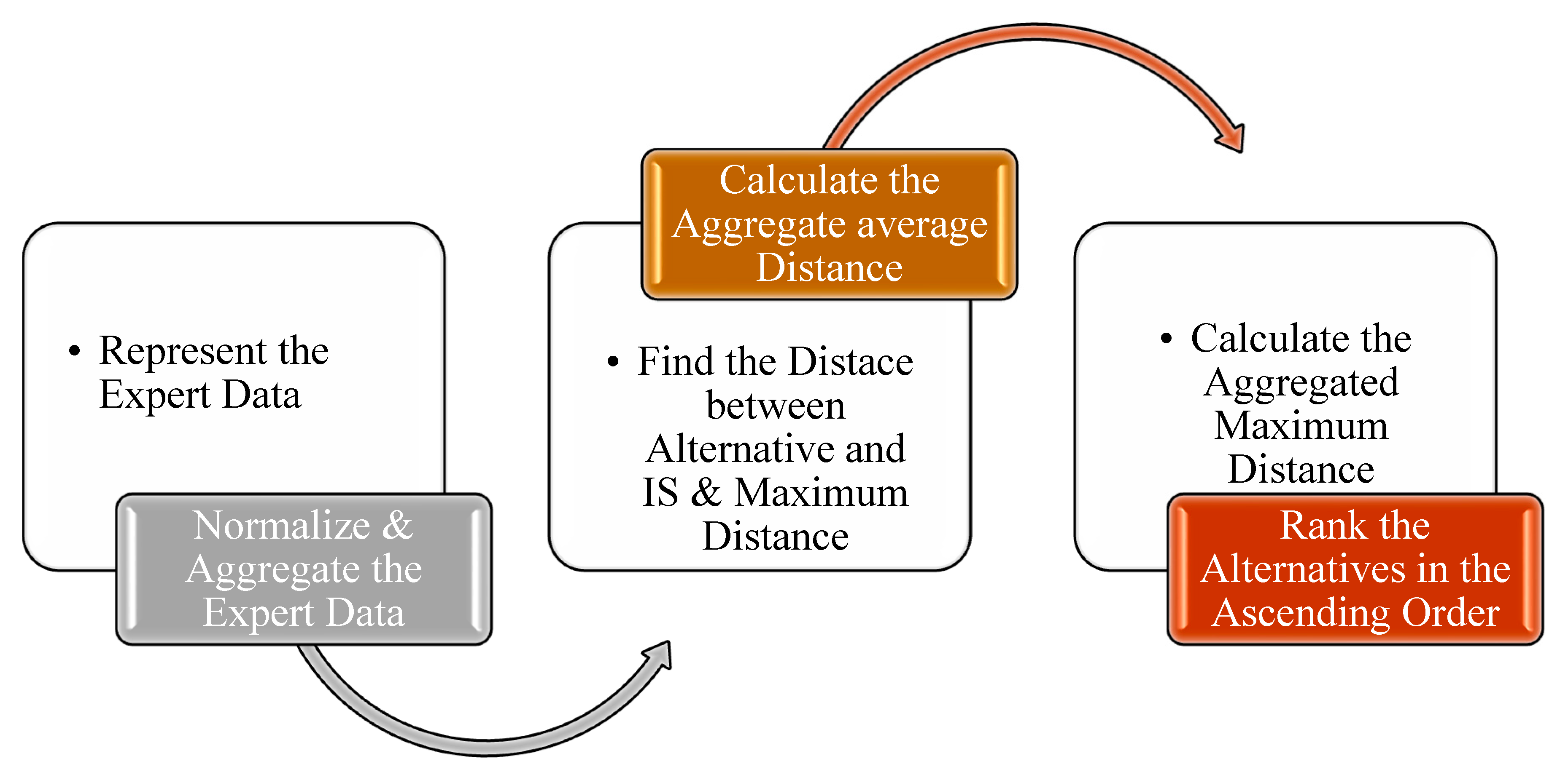
4. Methodology-I Proposed VIKOR Method for FFS Information

In 1998, Opricovic [31] introduced the VIKOR method as a multi-criteria decision-making (MCDM) method having multiple conflicting criteria involved. Over time, many scholars extended the VIKOR method to different extensions of FS. Now, we introduce the VIKOR approach in an FFS environment.

Let us consider that there are m alternatives ℑ$=\left\{{\mathfrak{I}}_1,{\mathfrak{I}}_2{,\mathfrak{I}}_3\dots {\mathfrak{I}}_{\mathrm{m}}\right\}$ and n criteria 𝔘$=\left\{{\mathfrak{U}}_1,{\mathfrak{U}}_2,{\mathfrak{U}}_3\dots {\mathfrak{U}}_{\mathrm{n}}\right\}$. Then, the expert decision matrices (DMs) can be represented by 𝔻 = ${\left({\mathbb{d}}_{\mathrm{i}\mathrm{j}}\right)}_{\mathrm{m}\times \mathrm{n}}$ and here ${\mathbb{d}}_{\mathrm{i}\mathrm{j}}$ be an attribute value of the alternative ${\mathfrak{I}}_{\mathrm{i}}$ under the attribute ${\mathfrak{U}}_{\mathrm{j}}$ where i $=1, 2, 3, \dots \mathrm{m}$ and j $=1, 2, 3, \dots$ n. The stepwise algorithm of the proposed FF-VIKOR method is given as follows:

Step-1. Collect information for decision matrices (DMs).

$$\mathbb{D}={\left({\mathbb{d}}_{\mathrm{i}\mathrm{j}}\right)}_{\mathrm{m}\times \mathrm{n}}=\begin{array}{c}{\mathfrak{I}}_1\\ \begin{array}{c}{\mathfrak{I}}_2\\ ⋮\end{array}\\ {\mathfrak{I}}_{\mathrm{m}}\end{array}\left(\begin{array}{ccc}\begin{array}{cc}{\mathbb{d}}_{11}& {\mathbb{d}}_{12}\end{array}& \cdots & {\mathbb{d}}_{1\mathrm{n}}\\ \begin{array}{cc}{\mathbb{d}}_{21}& {\mathbb{d}}_{22}\end{array}& \cdots & {\mathbb{d}}_{2\mathrm{n}}\\ \begin{array}{cc}⋮& ⋮\\ {\mathbb{d}}_{\mathrm{m}1}& {\mathbb{d}}_{\mathrm{m}2}\end{array}& \begin{array}{c}\ddots \\ \dots \end{array}& \begin{array}{c}⋮\\ {\mathbb{d}}_{\mathrm{m}\mathrm{n}}\end{array}\end{array}\right)$$

Step-2. Normalize the decision matrices (DMs).

Step-3. Using the proposed FFEWG aggregation operators (AoPs) to aggregate the DMs.

$$\begin{array}{c}{\mathrm{F}\mathrm{F}\mathrm{E}\mathrm{W}\mathrm{G}}_{\mathcal{w}}\left({\mathfrak{R}}_1,{\mathfrak{R}}_2,{\mathfrak{R}}_3,...,{\mathfrak{R}}_{\mathrm{n}}\right)=\hfill \\ \left(\frac{\sqrt[\mathbb{f}]{2}\prod _{\mathsf{\rho }=1}^{\mathrm{n}}{\left({{\tilde{\mathsf{\eta }}}_{{\mathfrak{R}}_{\mathsf{\rho }}}}^{\mathbb{f}}\right)}^{{\mathcal{w}}_{\mathsf{\rho }}}}{\sqrt[\mathbb{f}]{\prod _{\mathsf{\rho }=1}^{\mathrm{n}}{\left(2-{{\tilde{\mathsf{\eta }}}_{{\mathfrak{R}}_{\mathsf{\rho }}}}^{\mathbb{f}}\right)}^{{\mathcal{w}}_{\mathsf{\rho }}}+\prod _{\mathsf{\rho }=1}^{\mathrm{n}}{\left({{\tilde{\mathsf{\eta }}}_{{\mathfrak{R}}_{\mathsf{\rho }}}}^{\mathbb{f}}\right)}^{{\mathcal{w}}_{\mathsf{\rho }}}}},\frac{\sqrt[\mathbb{f}]{\prod _{\mathsf{\rho }=1}^{\mathrm{n}}{\left(1+{{\tilde{\upsilon }}_{{\mathfrak{R}}_{\mathsf{\rho }}}}^{\mathbb{f}}\right)}^{{\mathcal{w}}_{\mathsf{\rho }}}-\prod _{\mathsf{\rho }=1}^{\mathrm{n}}{\left(1-{{\tilde{\upsilon }}_{{\mathfrak{R}}_{\mathsf{\rho }}}}^{\mathbb{f}}\right)}^{{\mathcal{w}}_{\mathsf{\rho }}}}}{\sqrt[\mathbb{f}]{\prod _{\mathsf{\rho }=1}^{\mathrm{n}}{\left(1+{{\tilde{\upsilon }}_{{\mathfrak{R}}_{\mathsf{\rho }}}}^{\mathbb{f}}\right)}^{{\mathcal{w}}_{\mathsf{\rho }}}+\prod _{\mathsf{\rho }=1}^{\mathrm{n}}{\left(1-{{\tilde{\upsilon }}_{{\mathfrak{R}}_{\mathsf{\rho }}}}^{\mathbb{f}}\right)}^{{\mathcal{w}}_{\mathsf{\rho }}}}}\right).\hfill \end{array}$$

Step-4. From the decision matrix, calculate the positive ideal solution (PIS) and negative ideal solution (NIS) by the following equations.

$${\mathbb{d}}_{\mathrm{j}}^{+}=〈\underset{1\le \mathrm{i}\le \mathrm{m}}{\max }\left({\tilde{\mathsf{\eta }}}_{\mathrm{i}\mathrm{j}}\right),\underset{1\le \mathrm{i}\le \mathrm{m}}{\min }\left({\tilde{\upsilon }}_{\mathrm{i}\mathrm{j}}\right)〉=\left({\tilde{\mathsf{\eta }}}_{\mathrm{j}}^{+}{,\tilde{\upsilon }}_{\mathrm{j}}^{+}\right)$$

(24)

$${\mathbb{d}}_{\mathrm{j}}^{-}=〈\underset{1\le \mathrm{i}\le \mathrm{m}}{\min }\left({\tilde{\mathsf{\eta }}}_{\mathrm{i}\mathrm{j}}\right),\underset{1\le \mathrm{i}\le \mathrm{m}}{\max }\left({\tilde{\upsilon }}_{\mathrm{i}\mathrm{j}}\right)〉=\left({\tilde{\mathsf{\eta }}}_{\mathrm{j}}^{-}{,\tilde{\upsilon }}_{\mathrm{j}}^{-}\right)$$

(25)

Step-5. VIKOR Approach calculates the two primary distance measures. One is the distance between alternatives and ideal solutions denoted by ${\mathcal{S}}_i$ and the other ${\mathcal{R}}_i$ represents the maximum distance. Both are determined as follows,

$${\mathcal{S}}_{\mathrm{i}}={\sum }_{\mathrm{j}=1}^{\mathrm{n}}{\mathcal{w}}_{\mathrm{j}}\frac{{\mathrm{d}}_{\mathrm{e}\mathrm{u}}({\mathbb{d}}_{\mathrm{i}\mathrm{j}},{\mathbb{d}}_{\mathrm{j}}^{+})}{{\mathrm{d}}_{\mathrm{e}\mathrm{u}}({\mathbb{d}}_{\mathrm{j}}^{-},{\mathbb{d}}_{\mathrm{j}}^{+})}$$

(26)

$${\mathcal{R}}_{\mathrm{i}}=\underset{\mathrm{j}}{\max }\left({\mathcal{w}}_{\mathrm{j}}\frac{{\mathrm{d}}_{\mathrm{e}\mathrm{u}}({\mathbb{d}}_{\mathrm{i}\mathrm{j}},{\mathbb{d}}_{\mathrm{j}}^{+})}{{\mathrm{d}}_{\mathrm{e}\mathrm{u}}({\mathbb{d}}_{\mathrm{j}}^{-},{\mathbb{d}}_{\mathrm{j}}^{+})}\right)$$

(27)

where ${\mathrm{d}}_{\mathrm{e}\mathrm{u}}$ is the Euclidean distance between FFNs.

Step-6. Determine the aggregate average and maximum distance ${\mathfrak{Q}}_i$ by formula,

$${\mathfrak{Q}}_i=\gamma \frac{{\mathcal{S}}_i-\stackrel{̿}{\mathcal{S}}}{{\mathcal{S}}^{+}-\stackrel{̿}{\mathcal{S}}}+(1-\gamma )\frac{{\mathcal{R}}_i-\stackrel{̿}{\mathcal{R}}}{{\mathcal{R}}^{+}-\stackrel{̿}{\mathcal{R}}}$$

(28)

where $\stackrel{̿}{\mathcal{S}}=\underset{i}{\min }{\mathcal{S}}_i$, ${\mathcal{S}}^{+}=\underset{i}{\max }{\mathcal{S}}_i$, $\stackrel{̿}{\mathcal{R}}=\underset{i}{\min }{\mathcal{R}}_i$, ${\mathcal{R}}^{+}=\underset{i}{\max }{\mathcal{R}}_i$ and $\gamma$ are the weight for the procedure of maximum benefits and $\gamma$.

Step-7. Rank the alternatives in the ascending order ${\mathcal{S}}_{\mathrm{i}}$, ${\mathcal{R}}_{\mathrm{i}}$ and ${\mathfrak{Q}}_i$. The minimized value of ${\mathfrak{Q}}_i$ will be the best optimal alternative.

The graphical presentation of the proposed decision making method is given in Figure 1.

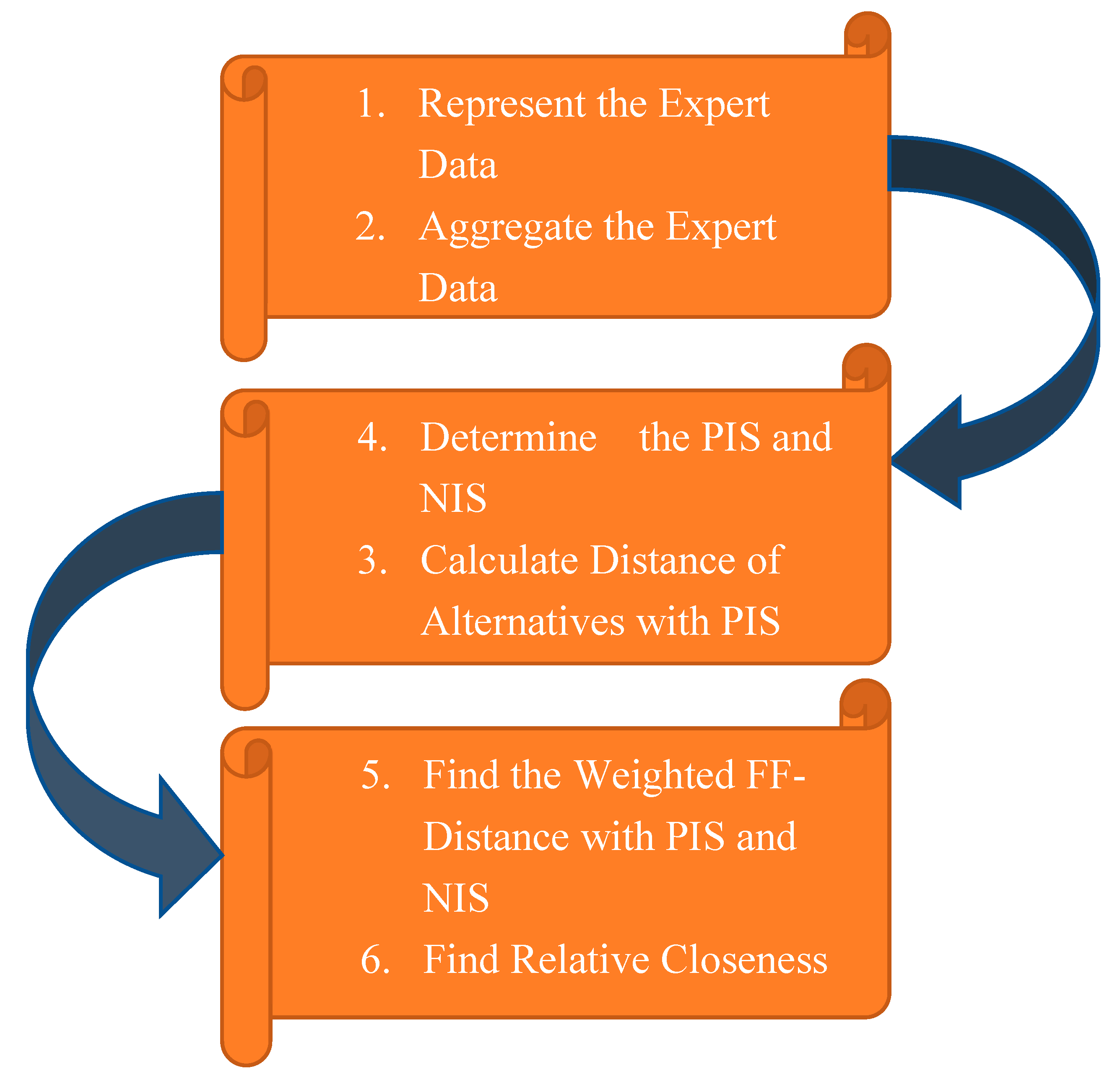
5. Methodology-II Proposed Extended TOPSIS Method for FFS Information

The detailed algorithm of the extended TOPSIS method is given as follows:

Step-1. Collect information for decision matrices (DMs). Generally,

$$\mathbb{D}={\left({\mathbb{d}}_{\mathrm{i}\mathrm{j}}\right)}_{\mathrm{m}\times \mathrm{n}}=\begin{array}{c}{\mathfrak{I}}_1\\ \begin{array}{c}{\mathfrak{I}}_2\\ ⋮\end{array}\\ {\mathfrak{I}}_{\mathrm{m}}\end{array}\left(\begin{array}{ccc}\begin{array}{cc}{\mathbb{d}}_{11}& {\mathbb{d}}_{12}\end{array}& \cdots & {\mathbb{d}}_{1\mathrm{n}}\\ \begin{array}{cc}{\mathbb{d}}_{21}& {\mathbb{d}}_{22}\end{array}& \cdots & {\mathbb{d}}_{2\mathrm{n}}\\ \begin{array}{cc}⋮& ⋮\\ {\mathbb{d}}_{\mathrm{m}1}& {\mathbb{d}}_{\mathrm{m}2}\end{array}& \begin{array}{c}\ddots \\ \dots \end{array}& \begin{array}{c}⋮\\ {\mathbb{d}}_{\mathrm{m}\mathrm{n}}\end{array}\end{array}\right)$$

Step-2. Using the proposed FFEWG aggregation operators (AoPs) to aggregate the DMs.

$$\begin{array}{c}{\mathrm{F}\mathrm{F}\mathrm{E}\mathrm{W}\mathrm{G}}_{\mathcal{w}}\left({\mathfrak{R}}_1,{\mathfrak{R}}_2,{\mathfrak{R}}_3,...,{\mathfrak{R}}_{\mathrm{n}}\right)=\hfill \\ \left(\frac{\sqrt[\mathbb{f}]{2}\prod _{\mathsf{\rho }=1}^{\mathrm{n}}{\left({{\tilde{\mathsf{\eta }}}_{{\mathfrak{R}}_{\mathsf{\rho }}}}^{\mathbb{f}}\right)}^{{\mathcal{w}}_{\mathsf{\rho }}}}{\sqrt[\mathbb{f}]{\prod _{\mathsf{\rho }=1}^{\mathrm{n}}{\left(2-{{\tilde{\mathsf{\eta }}}_{{\mathfrak{R}}_{\mathsf{\rho }}}}^{\mathbb{f}}\right)}^{{\mathcal{w}}_{\mathsf{\rho }}}+\prod _{\mathsf{\rho }=1}^{\mathrm{n}}{\left({{\tilde{\mathsf{\eta }}}_{{\mathfrak{R}}_{\mathsf{\rho }}}}^{\mathbb{f}}\right)}^{{\mathcal{w}}_{\mathsf{\rho }}}}},\frac{\sqrt[\mathbb{f}]{\prod _{\mathsf{\rho }=1}^{\mathrm{n}}{\left(1+{{\tilde{\upsilon }}_{{\mathfrak{R}}_{\mathsf{\rho }}}}^{\mathbb{f}}\right)}^{{\mathcal{w}}_{\mathsf{\rho }}}-\prod _{\mathsf{\rho }=1}^{\mathrm{n}}{\left(1-{{\tilde{\upsilon }}_{{\mathfrak{R}}_{\mathsf{\rho }}}}^{\mathbb{f}}\right)}^{{\mathcal{w}}_{\mathsf{\rho }}}}}{\sqrt[\mathbb{f}]{\prod _{\mathsf{\rho }=1}^{\mathrm{n}}{\left(1+{{\tilde{\upsilon }}_{{\mathfrak{R}}_{\mathsf{\rho }}}}^{\mathbb{f}}\right)}^{{\mathcal{w}}_{\mathsf{\rho }}}+\prod _{\mathsf{\rho }=1}^{\mathrm{n}}{\left(1-{{\tilde{\upsilon }}_{{\mathfrak{R}}_{\mathsf{\rho }}}}^{\mathbb{f}}\right)}^{{\mathcal{w}}_{\mathsf{\rho }}}}}\right).\hfill \end{array}$$

Step-3. From the decision matrix, calculate the positive ideal solution (PIS) and negative ideal solution (NIS) by the following equations.

$${\mathbb{d}}_{\mathrm{j}}^{+}=〈\underset{1\le \mathrm{i}\le \mathrm{m}}{\max }\left({\tilde{\mathsf{\eta }}}_{\mathrm{i}\mathrm{j}}\right),\underset{1\le \mathrm{i}\le \mathrm{m}}{\min }\left({\tilde{\upsilon }}_{\mathrm{i}\mathrm{j}}\right)〉=\left({\tilde{\mathsf{\eta }}}_{\mathrm{j}}^{+}{,\tilde{\upsilon }}_{\mathrm{j}}^{+}\right)$$

(29)

$${\mathbb{d}}_{\mathrm{j}}^{-}=〈\underset{1\le \mathrm{i}\le \mathrm{m}}{\min }\left({\tilde{\mathsf{\eta }}}_{\mathrm{i}\mathrm{j}}\right),\underset{1\le \mathrm{i}\le \mathrm{m}}{\max }\left({\tilde{\upsilon }}_{\mathrm{i}\mathrm{j}}\right)〉=\left({\tilde{\mathsf{\eta }}}_{\mathrm{j}}^{-}{,\tilde{\upsilon }}_{\mathrm{j}}^{-}\right)$$

(30)

Step-4. Find out the distance of each alternative with FF-PIS and FF-NIS employing the following normalized Euclidean distance formula among FFNs;

$$\mathbb{D}({\mathbb{d}}_{\mathrm{j}},{\mathbb{d}}_{\mathrm{j}}^{+})=\sqrt{{\left({{\tilde{\mathsf{\eta }}}_{\mathbb{d}}}^{\mathbb{f}}-{{\tilde{\mathsf{\eta }}}_{{\mathbb{d}}_{\mathrm{j}}^{+}}}^{\mathbb{f}}\right)}^2+{\left({{\tilde{\upsilon }}_{\mathbb{d}}}^{\mathbb{f}}-{{\tilde{\upsilon }}_{{\mathbb{d}}_{\mathrm{j}}^{+}}}^{\mathbb{f}}\right)}^2+{\left({{\mathsf{\pi }}_{\mathbb{d}}}^{\mathbb{f}}-{{\mathsf{\pi }}_{{\mathbb{d}}_{\mathrm{j}}^{+}}}^{\mathbb{f}}\right)}^2}$$

(31)

We can obtain the following two fractional fuzzy distance matrices;

$${\mathbb{D}}^{+}={({\mathbb{d}}_{\mathrm{i}\mathrm{j}},{\mathbb{d}}_{\mathrm{j}}^{+})}_{\mathrm{m}\times \mathrm{n}}=\begin{array}{c}{\mathfrak{I}}_1\\ \begin{array}{c}{\mathfrak{I}}_2\\ ⋮\end{array}\\ {\mathfrak{I}}_{\mathrm{m}}\end{array}\left(\begin{array}{ccc}\begin{array}{cc}\mathrm{d}({\mathbb{d}}_{11},{\mathbb{d}}_1^{+})& \mathrm{d}({\mathbb{d}}_{12},{\mathbb{d}}_2^{+})\end{array}& \cdots & \mathrm{d}({\mathbb{d}}_{1\mathrm{n}},{\mathbb{d}}_{\mathrm{n}}^{+})\\ \begin{array}{cc}\mathrm{d}({\mathbb{d}}_{21},{\mathbb{d}}_2^{+})& \mathrm{d}({\mathbb{d}}_{22},{\mathbb{d}}_2^{+})\end{array}& \cdots & \mathrm{d}({\mathbb{d}}_{2\mathrm{n}},{\mathbb{d}}_{\mathrm{n}}^{+})\\ \begin{array}{cc}⋮& ⋮\\ \mathrm{d}({\mathbb{d}}_{\mathrm{m}1},{\mathbb{d}}_{\mathrm{m}}^{+})& \mathrm{d}({\mathbb{d}}_{\mathrm{m}2},{\mathbb{d}}_{\mathrm{m}}^{+})\end{array}& \begin{array}{c}\ddots \\ \dots \end{array}& \begin{array}{c}⋮\\ \mathrm{d}({\mathbb{d}}_{\mathrm{m}\mathrm{n}},{\mathbb{d}}_{\mathrm{n}}^{+})\end{array}\end{array}\right)$$

$${\mathbb{D}}^{-}={({\mathbb{d}}_{\mathrm{i}\mathrm{j}},{\mathbb{d}}_{\mathrm{j}}^{-})}_{\mathrm{m}\times \mathrm{n}}=\begin{array}{c}{\mathfrak{I}}_1\\ \begin{array}{c}{\mathfrak{I}}_2\\ ⋮\end{array}\\ {\mathfrak{I}}_{\mathrm{m}}\end{array}\left(\begin{array}{ccc}\begin{array}{cc}\mathrm{d}({\mathbb{d}}_{11},{\mathbb{d}}_1^{-})& \mathrm{d}({\mathbb{d}}_{12},{\mathbb{d}}_2^{-})\end{array}& \cdots & \mathrm{d}({\mathbb{d}}_{1\mathrm{n}},{\mathbb{d}}_{\mathrm{n}}^{-})\\ \begin{array}{cc}\mathrm{d}({\mathbb{d}}_{21},{\mathbb{d}}_2^{-})& \mathrm{d}({\mathbb{d}}_{22},{\mathbb{d}}_2^{-})\end{array}& \cdots & \mathrm{d}({\mathbb{d}}_{2\mathrm{n}},{\mathbb{d}}_{\mathrm{n}}^{-})\\ \begin{array}{cc}⋮& ⋮\\ \mathrm{d}({\mathbb{d}}_{\mathrm{m}1},{\mathbb{d}}_{\mathrm{m}}^{-})& \mathrm{d}({\mathbb{d}}_{\mathrm{m}2},{\mathbb{d}}_{\mathrm{m}}^{-})\end{array}& \begin{array}{c}\ddots \\ \dots \end{array}& \begin{array}{c}⋮\\ \mathrm{d}({\mathbb{d}}_{\mathrm{m}\mathrm{n}},{\mathbb{d}}_{\mathrm{n}}^{-})\end{array}\end{array}\right)$$

Step-5. Calculate the weight of the aggregated table and then deduce the weighted fractional fuzzy distance of all alternatives with PIS and NIS. We can represent as,

$${\mathsf{\Lambda }}_{\mathrm{i}}^{\mathrm{*}}={\sum }_{\mathrm{j}=1}^{\mathrm{n}}{\mathcal{w}}_{\mathrm{j}}{{\mathbb{D}}^{\mathrm{*}}}_{\mathrm{j}},\mathrm{i}=1, 2, 3,\dots ,\mathrm{ᵹ}, \mathrm{where} (\ast =+\mathrm{o}\mathrm{r}-)$$

(32)

Step-6. Deduce the relative closeness (RC) index of all alternatives ${\mathfrak{I}}_{\mathrm{i}}$ as below;

$${\mathsf{\zeta }}_i^{+}=\frac{{\mathsf{\Lambda }}^{+}({\mathbb{d}}_{\mathrm{i}\mathrm{j}},{\mathbb{d}}_{\mathrm{j}}^{+})}{\left({\mathsf{\Lambda }}^{+}({\mathbb{d}}_{\mathrm{i}},{\mathbb{d}}_{\mathrm{j}}^{+}){+\mathsf{\Lambda }}^{-}({\mathbb{d}}_{\mathrm{i}\mathrm{j}},{\mathbb{d}}_{\mathrm{j}}^{-})\right)}$$

Step-7. Ranking. Bigger the value of ${\mathsf{\zeta }}_i^{+}$ will be the best optimal alternative ${\mathfrak{I}}_{\mathrm{i}}$.

The flow chart of the proposed algorithm-II is given in Figure 2.

6. Real Life Decision Making Problem

In this section, we provide a case study of the evaluation of artificial intelligence cloud platforms. We recommend the VIKOR method and the extended TOPSIS method to make decisions and rank the alternatives, and we compare them with other existing approaches.

Case Study

At the end of 2022, this analysis was initiated when numerous round-table sessions with stakeholders were scheduled. A specialist panel contributed to generating the eligibility standards and possible outcomes for a decision. Members of the panel were chosen from a group of outstanding and competent people depending on an assortment of parameters.

Scholars demonstrated that the main advantage was expertise in the AI-cloud service sector. The second most crucial factor was professional managerial knowledge (minimum of five years as a prominent supervisor), and the third was membership in the company’s management team. These renowned individuals took part in a physical debate that included broad inquiries before developing a set of the necessary attributes and alternatives for assessing implications parameters utilizing the AICP ratings. After the collection of the above lists, the same chosen attribute and options were eliminated, allowing the last decision to be purely attributable to the options available.

Table 1. Informastion of decision experts.

DMs	Responsibilities	Major	Association	Years of Experience	Level of Education
1	Enterprise owner	IT Supervision and Software Engineer	Member of Council	20	Postdoc
2	AI Developer	IT Supervision and Big Data Expert	Member of Council	14	PhD
3	Experienced Big Data Expert/Architect	IT Supervision and Big Data Scientist	Member of Council	12	PhD

contains the names of the specialists who are part of the committee.

The inspection of crucial AICP factors not only assists big enterprises but also offers important customer service and financial advantages. Most AI service provider companies offer substantial deep data science, machine learning platforms, and API services. Therefore, an AI cloud can save time and assets for companies. However, AI cloud evolution is incomplete until it transforms into highly innovative enterprises or, more precisely, into the digital businesses of the next generation. To create such an environment of unbounded innovation, the transition of AICPs must give the most importance to six crucial operations. Additionally, promoting development, the most significant issues confronting enterprises in the coming year could be managed with support from the AI cloud, including chip shortages and increasing energy prices, which affect every aspect, including hardware purchases and business continuity. In the future, AI cloud providers and analytics organizations can enhance these services in the AICP. AI clouds and their subdomains are the primary drivers of the rapid expansion of technological ecosystems. Gartner defines AI cloud as the use of “advanced analysis and logic-based techniques” to replicate human intelligence. AI clouds offer various applications to individuals and businesses across industries. User organizations and their technology partners frequently design, customize, and operate AI cloud implementations in many prominent AICPs. Given the worldwide expansion of AI software, these systems are crucial. Gartner projected the market to reach $62.5 billion in 2022, a 21.3% rise from its value in 2021. International Data Corporation anticipates this market to reach $549.9 billion by 2025. The evaluation of AICP involves many critical functions, such as ${\mathfrak{U}}_1$ smart robotics, ${\mathfrak{U}}_2$ the capacity to prototype and test applications rapidly and affordably (lower costs), ${\mathfrak{U}}_3$ higher and more effective digital security, ${\mathfrak{U}}_4$ simply integration into the operational and security environment of other applications currently supported in the enterprise (broader perspectives), ${\mathfrak{U}}_5$ the ability to rapidly scale up from prototype to large-scale analysis and computation environments, and ${\mathfrak{U}}_6$ optimal management of data. Furthermore, the weights of the three decision-makers were ${\mathbf{D}}^{\mathbf{m}}$ = (0.32, 0.34, 0.34). Decision matrices of three DMs for FFSs.

Determining the best optimal alternative, we adopted the suggested strategy to speed up the selection.

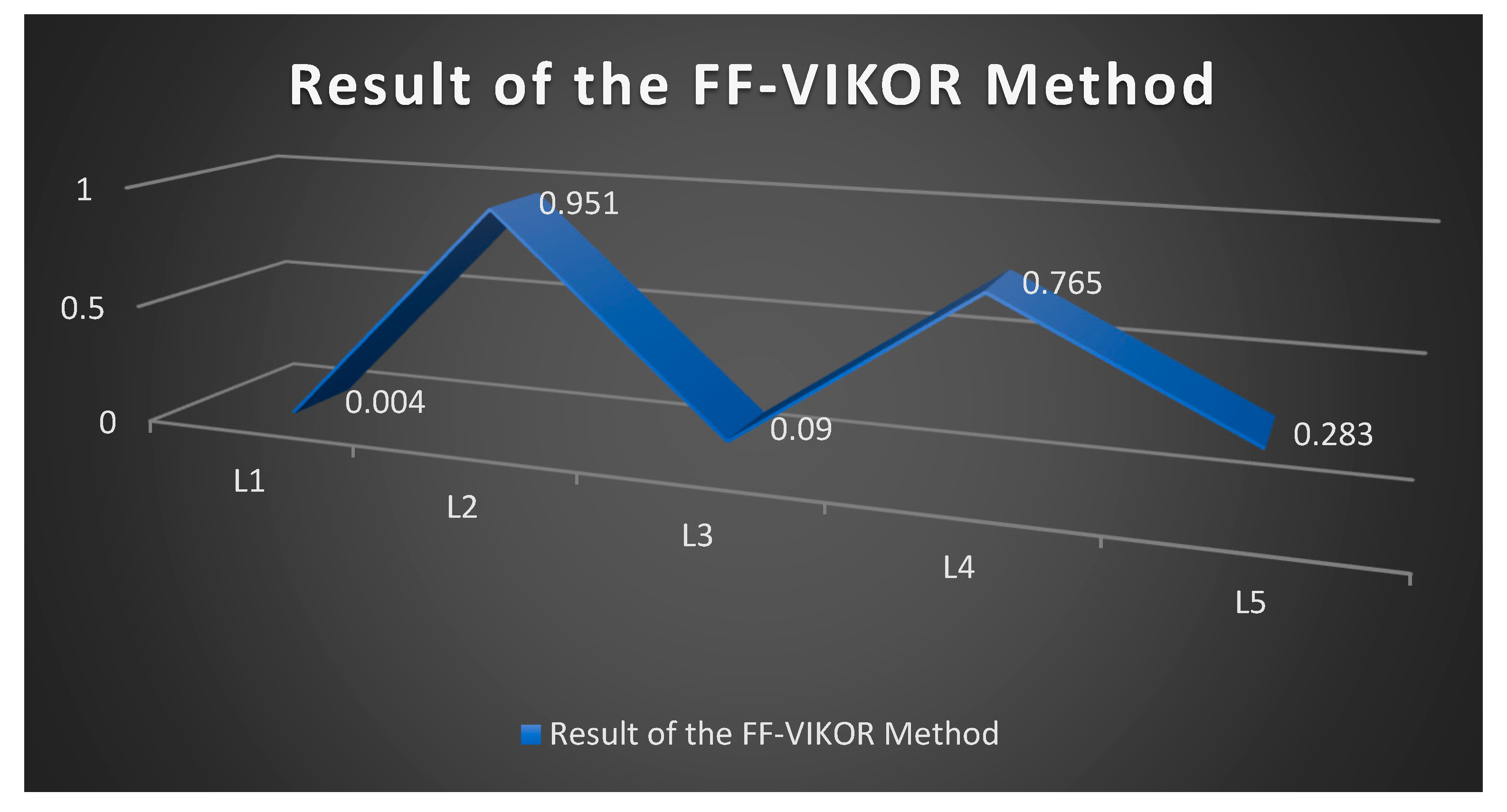
7. Numerical Result of the Proposed VIKOR Method for FFS information

Step-1. Collect the expert information in the form of DMs for FFNs. The detail of all decision epert are giving

Table 2. Expert Data-2.

Alternatives	${\mathfrak{U}}_1$	${\mathfrak{U}}_2$	${\mathfrak{U}}_3$	${\mathfrak{U}}_4$	${\mathfrak{U}}_5$	${\mathfrak{U}}_6$
${\mathfrak{I}}_1$	(0.8,0.5)	(0.9,0.3)	(0.7,0.5)	(0.2,0.6)	(0.2,0.4)	(0.3,0.2)
${\mathfrak{I}}_2$	(0.3,0.7)	(0.7,0.4)	(0.1,0.4)	(0.3,0.4)	(0.4,0.3)	(0.6,0.4)
${\mathfrak{I}}_3$	(0.4,0.1)	(0.2,0.6)	(0.3,0.8)	(0.6,0.2)	(0.3,0.4)	(0.4,0.1)
${\mathfrak{I}}_4$	(0.1,0.6)	(0.5,0.8)	(0.6,0.4)	(0.2,0.8)	(0.4,0.1)	(0.1,0.9)
${\mathfrak{I}}_5$	(0.3,0.9)	(0.1,0.3)	(0.2,0.6)	(0.3,0.5)	(0.4,0.5)	(0.5,0.7)

,

Table 3. Expert Data-3.

Alternatives	${\mathfrak{U}}_1$	${\mathfrak{U}}_2$	${\mathfrak{U}}_3$	${\mathfrak{U}}_4$	${\mathfrak{U}}_5$	${\mathfrak{U}}_6$
${\mathfrak{I}}_1$	(0.7,0.4)	(0.8,0.5)	(0.6,0.9)	(0.1,0.4)	(0.1,0.2)	(0.3,0.7)
${\mathfrak{I}}_2$	(0.4,0.2)	(0.4,0.4)	(0.6,0.2)	(0.5,0.7)	(0.5,0.9)	(0.2,0.4)
${\mathfrak{I}}_3$	(0.5,0.4)	(0.2,0.2)	(0.4,0.1)	(0.3,0.3)	(0.4,0.2)	(0.4,0.2)
${\mathfrak{I}}_4$	(0.1,0.9)	(0.3,0.1)	(0.2,0.4)	(0.4,0.7)	(0.3,0.5)	(0.5,0.1)
${\mathfrak{I}}_5$	(0.8,0.3)	(0.1,0.5)	(0.8,0.7)	(0.2,0.1)	(0.7,0.4)	(0.6,0.7)

and

Table 4. Expert Data-4.

Alternatives	${\mathfrak{U}}_1$	${\mathfrak{U}}_2$	${\mathfrak{U}}_3$	${\mathfrak{U}}_4$	${\mathfrak{U}}_5$	${\mathfrak{U}}_6$
${\mathfrak{I}}_1$	(0.6,0.3)	(0.3,0.4)	(0.9,0.3)	(0.1,0.8)	(0.3,0.4)	(0.7,0.1)
${\mathfrak{I}}_2$	(0.2,0.)	(0.5,0.2)	(0.7,0.4)	(0.2,0.6)	(0.4,0.6)	(0.2,0.9)
${\mathfrak{I}}_3$	(0.3,0.1)	(0.7,0.6)	(0.3,0.7)	(0.3,0.4)	(0.4,0.1)	(0.3,0.2)
${\mathfrak{I}}_4$	(0.6,0.9)	(0.1,0.8)	(0.4,0.1)	(0.4,0.3)	(0.2,0.6)	(0.4,0.5)
${\mathfrak{I}}_5$	(0.1,0.5)	(0.4,0.3)	(0.1,0.3)	(0.6,0.4)	(0.4,0.4)	(0.9,0.3)

.

Step-2. No need for normalization as all data are uniform.

Step-3. Aggregate these expert data using Equation (7).

The detail information of aggregated data of all expert are given in

Table 5. Result of the aggregated expert data.

Alternatives	${\mathfrak{U}}_1$	${\mathfrak{U}}_2$	${\mathfrak{U}}_3$	${\mathfrak{U}}_4$	${\mathfrak{U}}_5$	${\mathfrak{U}}_6$
${\mathfrak{I}}_1$	(0.533,0.394)	(0.501,0.382)	(0.546,0.680)	(0.124,0.519)	(0.178,0.309)	(0.369,0.462)
${\mathfrak{I}}_2$	(0.276,0.502)	(0.445,0.342)	(0.341,0.309)	(0.296,0.539)	(0.387,0.673)	(0.276,0.472)
${\mathfrak{I}}_3$	(0.359,0.258)	(0.296,0.446)	(0.311,0.575)	(0.348,0.269)	(0.338,0.269)	(0.337,0.157)
${\mathfrak{I}}_4$	(0.184,0.745)	0.239,0.590)	(0.338,0.337)	(0.303,0.653)	(0.275,0.394)	(0.268,0.641)
${\mathfrak{I}}_5$	(0.286,0.654)	(0.158,0.368)	(0.254,0.564)	(0.314,0.347)	(0.425.0.407)	(0.517,0.603)

and the weight information are given

Table 6. Weight of the aggregated table.

Criteria	${\mathfrak{U}}_1$	${\mathfrak{U}}_2$	${\mathfrak{U}}_3$	${\mathfrak{U}}_4$	${\mathfrak{U}}_5$	${\mathfrak{U}}_6$
	0.1527	0.2038	0.1022	0.1494	0.2482	0.1437

.

Step-4. Calculate the PIS and NIS using Equations (24) and (25). The PIS and NIS are given in

Table 7. Result of the PIS and NIS ${\mathbb{d}}_{\mathrm{j}}^{+}$ (j= 1, 2… 6).

${\mathbb{d}}_{\mathbf{j}}^{+}$	${\mathbb{d}}_1^{+}$	${\mathbb{d}}_2^{+}$	${\mathbb{d}}_3^{+}$	${\mathbb{d}}_4^{+}$	${\mathbb{d}}_5^{+}$	${\mathbb{d}}_6^{+}$
	(0.532,0.258)	(0.501,0.342)	(0.546,0.309)	(0.348,0.269)	(0.425,0.269)	(0.517,0.157)
${\mathbb{d}}_{\mathbf{j}}^{-}$	${\mathbb{d}}_1^{-}$	${\mathbb{d}}_2^{-}$	${\mathbb{d}}_3^{-}$	${\mathbb{d}}_4^{-}$	${\mathbb{d}}_5^{-}$	${\mathbb{d}}_6^{-}$
	(0.183,0.745)	(0.158,0.590)	(0.254,0.680)	(0.124,0.653)	(0.178,0.673)	(0.286,0.641)

.

Step-5. Calculate the Distances. The distance measure given in

Table 8. Result of the distance between alternative and ideal solution ${\mathcal{S}}_i$ (i= 1, 2… 5) by (26).

${\mathcal{S}}_{\mathbf{i}}$	${\mathcal{S}}_1$	${\mathcal{S}}_2$	${\mathcal{S}}_3$	${\mathcal{S}}_4$	${\mathcal{S}}_5$
	0.378	0.655	0.359	0.763	0.524

and the maximum distance measure are given in

Table 9. Result of the maximum distance ${\mathcal{R}}_{\mathrm{i}}$ (i= 1, 2… 5) by (27).

${\mathcal{R}}_{\mathbf{i}}$	${\mathcal{R}}_1$	${\mathcal{R}}_2$	${\mathcal{R}}_3$	${\mathcal{R}}_4$	${\mathcal{R}}_5$
	0.101	0.225	0.114	0.193	0.135

.

Step-6. Calculate the average and maximum distance by (28) and given in

Table 10. Result of the average and maximum distance ${\mathfrak{Q}}_i$.

${\mathfrak{Q}}_{\mathbf{i}}$	${\mathfrak{Q}}_1$	${\mathfrak{Q}}_2$	${\mathfrak{Q}}_3$	${\mathfrak{Q}}_4$	${\mathfrak{Q}}_5$
	0.004	0.951	0.090	0.765	0.283

.

Step-7. Ranking. Minimum the value of ${\mathfrak{Q}}_i$ will be the best optimal alternative. The ranking information are given in

Table 11. Ranking.

Alternatives

${\mathfrak{I}}_1\succ {\mathfrak{I}}_3\succ {\mathfrak{I}}_5\succ {\mathfrak{I}}_4\succ {\mathfrak{I}}_2$

. The graphical presentation of the ranking re given in Figure 3.

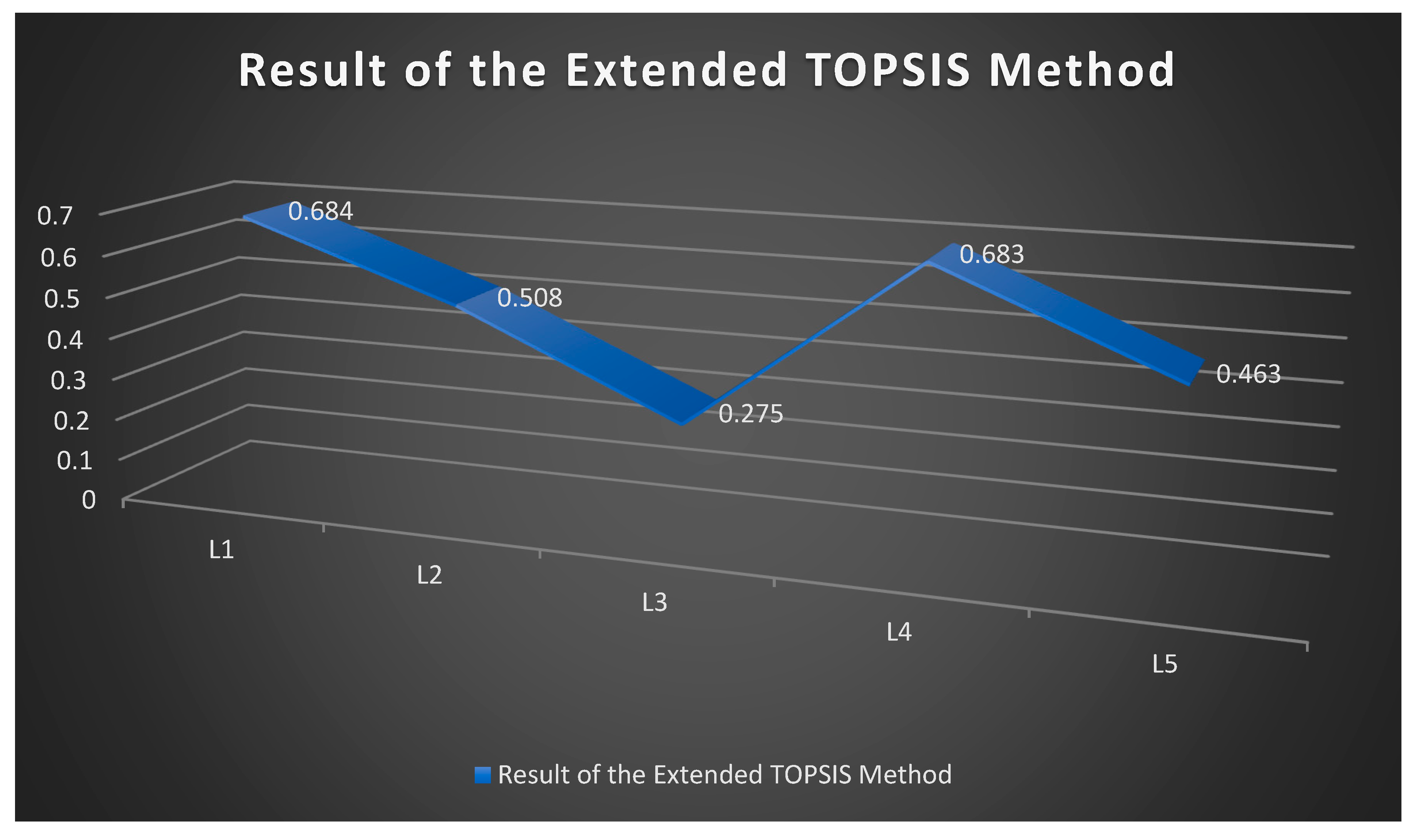
8. Numerical Results of Our Proposed Extended TOPSIS Method for FFS information

Step-1. Represent Table 1, Table 2, and Table 3 same as methodology-I.

Step-2. Using the proposed FFEWG aggregation operators (AoPs) to aggregate the DMs.

$$\begin{array}{c}{\mathrm{F}\mathrm{F}\mathrm{E}\mathrm{W}\mathrm{G}}_{\mathcal{w}}\left({\mathfrak{R}}_1,{\mathfrak{R}}_2,{\mathfrak{R}}_3,...,{\mathfrak{R}}_{\mathrm{n}}\right)=\hfill \\ \left(\frac{\sqrt[\mathbb{f}]{2}\prod _{\mathsf{\rho }=1}^{\mathrm{n}}{\left({{\tilde{\mathsf{\eta }}}_{{\mathfrak{R}}_{\mathsf{\rho }}}}^{\mathbb{f}}\right)}^{{\mathcal{w}}_{\mathsf{\rho }}}}{\sqrt[\mathbb{f}]{\prod _{\mathsf{\rho }=1}^{\mathrm{n}}{\left(2-{{\tilde{\mathsf{\eta }}}_{{\mathfrak{R}}_{\mathsf{\rho }}}}^{\mathbb{f}}\right)}^{{\mathcal{w}}_{\mathsf{\rho }}}+\prod _{\mathsf{\rho }=1}^{\mathrm{n}}{\left({{\tilde{\mathsf{\eta }}}_{{\mathfrak{R}}_{\mathsf{\rho }}}}^{\mathbb{f}}\right)}^{{\mathcal{w}}_{\mathsf{\rho }}}}},\frac{\sqrt[\mathbb{f}]{\prod _{\mathsf{\rho }=1}^{\mathrm{n}}{\left(1+{{\tilde{\upsilon }}_{{\mathfrak{R}}_{\mathsf{\rho }}}}^{\mathbb{f}}\right)}^{{\mathcal{w}}_{\mathsf{\rho }}}-\prod _{\mathsf{\rho }=1}^{\mathrm{n}}{\left(1-{{\tilde{\upsilon }}_{{\mathfrak{R}}_{\mathsf{\rho }}}}^{\mathbb{f}}\right)}^{{\mathcal{w}}_{\mathsf{\rho }}}}}{\sqrt[\mathbb{f}]{\prod _{\mathsf{\rho }=1}^{\mathrm{n}}{\left(1+{{\tilde{\upsilon }}_{{\mathfrak{R}}_{\mathsf{\rho }}}}^{\mathbb{f}}\right)}^{{\mathcal{w}}_{\mathsf{\rho }}}+\prod _{\mathsf{\rho }=1}^{\mathrm{n}}{\left(1-{{\tilde{\upsilon }}_{{\mathfrak{R}}_{\mathsf{\rho }}}}^{\mathbb{f}}\right)}^{{\mathcal{w}}_{\mathsf{\rho }}}}}\right).\hfill \end{array}$$

Step-3. Calculate PIS and NIS Same as Table 6 of methodology-I.

Step-4. Calculate distances with PIS and NIS Equation (31). The result is given in

Table 12. Result of Distance with PIS ${\mathbb{D}}^{+}$.

Alternatives	${\mathbb{d}}_1^{+}$	${\mathbb{d}}_2^{+}$	${\mathbb{d}}_3^{+}$	${\mathbb{d}}_4^{+}$	${\mathbb{d}}_5^{+}$	${\mathbb{d}}_6^{+}$
${\mathfrak{I}}_1$	0.075	0.037	0.341	0.659	0.114	0.998
${\mathfrak{I}}_2$	0.206	0.053	0.129	0.193	0.351	0.203
${\mathfrak{I}}_3$	0.116	0.130	0.247	0.062	0.075	0.121
${\mathfrak{I}}_4$	0.486	0.241	0.130	0.324	0.106	0.362
${\mathfrak{I}}_5$	0.352	0.149	0.246	0.070	0.084	0.295

and

Table 13. Result of Distance with NIS ${\mathbb{D}}^{-}$.

Alternatives	${\mathbb{d}}_1^{-}$	${\mathbb{d}}_2^{-}$	${\mathbb{d}}_3^{-}$	${\mathbb{d}}_4^{-}$	${\mathbb{d}}_5^{-}$	${\mathbb{d}}_6^{-}$
${\mathfrak{I}}_1$	0.418	0.229	0.143	0.159	0.003	0.002
${\mathfrak{I}}_2$	0.307	0.235	0.348	0.141	0.065	0.185
${\mathfrak{I}}_3$	0.469	0.150	0.133	0.334	0.359	0.350
${\mathfrak{I}}_4$	0.007	0.030	0.333	0.040	0.290	0.017
${\mathfrak{I}}_5$	0.136	0.206	0.146	0.294	0.289	0.128

.

Step-5. Calculate the weighted Fractional fuzzy distance of all alternatives with PIS and NIS by Equation (32) and information is given in

Table 14. Result of the weighted distance with PIS ${\mathsf{\Lambda }}_{\mathrm{i}}^{+}$ (i= 1, 2… 5).

${\mathsf{\Lambda }}_{\mathbf{i}}^{+}$	${\mathsf{\Lambda }}_1^{+}$	${\mathsf{\Lambda }}_2^{+}$	${\mathsf{\Lambda }}_3^{+}$	${\mathsf{\Lambda }}_4^{+}$	${\mathsf{\Lambda }}_5^{+}$
	0.324	0.201	0.115	0.263	0.183

and

Table 15. Result of the weighted distance with NIS ${\mathsf{\Lambda }}_{\mathrm{i}}^{-}$ (i= 1, 2… 5).

${\mathsf{\Lambda }}_{\mathbf{i}}^{-}$	${\mathsf{\Lambda }}_1^{-}$	${\mathsf{\Lambda }}_2^{-}$	${\mathsf{\Lambda }}_3^{-}$	${\mathsf{\Lambda }}_4^{-}$	${\mathsf{\Lambda }}_5^{-}$
	0.149	0.194	0.305	0.122	0.212

.

Step-6. Determine the relative closeness indices ${\mathsf{\zeta }}_i^{+}$ by Equation (33) and information is given in

Table 16. Result of the RC.

${\mathsf{\zeta }}_{\mathit{i}}^{+}$	${\mathsf{\zeta }}_1^{+}$	${\mathsf{\zeta }}_2^{+}$	${\mathsf{\zeta }}_3^{+}$	${\mathsf{\zeta }}_4^{+}$	${\mathsf{\zeta }}_5^{+}$
	0.684	0.508	0.274	0.683	0.463

.

Step-7. Rank the alternatives ${\mathfrak{I}}_{\mathrm{i}}$. The bigger value of the alternative will be the most optimal and the details are given in

Table 17. Ranking.

Alternatives

${\mathfrak{I}}_1\succ {\mathfrak{I}}_4\succ {\mathfrak{I}}_2\succ {\mathfrak{I}}_5\succ {\mathfrak{I}}_3$

. The graphical view of the proposed Extended TOPSIS method is given in Figure 4.

9. Comparative Analysis and Discussion

In this section, we can compare the proposed method with the extended GRA, and the calculation of alternative scores was performed by the well-known extended GRA method by Khan, Abdullah (2018) [32] to check the stability, validity, and correctness of the proposed methods.

Moreover, our suggested operators possess a broad variety of practicality because of the availability of parameter $\mathbb{f}=\mathbb{p}/\mathbb{q}.$ Under FFS circumstances, we construct a systematic comparison between our proposed Einstein geometric aggregation operators (AoPs) and the extended TOPSIS approach and VIKOR approach with the existing PyF extended GRA approach [32]. To analyze the results obtained utilizing the existing approach, first, we determine the expert data for assessment. After that, we must give each criterion a weight to illustrate their order of importance. These weights can be obtained by decision maker (DM) importance or by applying the entropy measure. Once the weights and criteria are determined, we examine each alternative to each criterion. Implementing the PyF extended GRA methodology to rank the alternatives. In light of the distinctive characteristics of the PyF extended GRA approach, different outcomes were attained while processing the exact initial data. Despite the fact that these suggested approaches’ results are different from the existing approaches, the optimal alternative is always the same ${\mathfrak{I}}_1$.

The results of the comparison are demonstrated in

Table 18. Result of comparison.

Various Approaches	Score Values
Extended GRA Method [32]	0.252	0.185	0.108	0.128	0.084
Proposed FF-VIKOR Method	0.004	0.951	0.090	0.765	0.283
Proposed FF-Extended TOPSIS Method	0.684	0.508	0.274	0.683	0.463

as follows and overall result is given in

Table 19. Overall Ranking.

Various Approaches	Ranking
Existing GRA Method [32]	${\mathfrak{I}}_1\succ {\mathfrak{I}}_2\succ {\mathfrak{I}}_3\succ {\mathfrak{I}}_4\succ {\mathfrak{I}}_5$
Proposed FF-VIKOR Method	${\mathfrak{I}}_1\succ {\mathfrak{I}}_3\succ {\mathfrak{I}}_5\succ {\mathfrak{I}}_4\succ {\mathfrak{I}}_2$
Proposed FF-Extended TOPSIS Method	${\mathfrak{I}}_1\succ {\mathfrak{I}}_4\succ {\mathfrak{I}}_2\succ {\mathfrak{I}}_5\succ {\mathfrak{I}}_3$

.

10. Conclusions and Future Research Directions

The efficiency of the recommended FF-VIKOR technique and FF-Extended TOPSIS technique were analyzed. In this study, the FF–VIKOR approach and the FF-Extended TOPSIS approach were used for MCGDM using FFSs. Detailed illustrations of AICP assessment and comparison analysis were employed to verify the sustainability of this novel approach. The following are consequences of the broadened model: The FF–VIKOR technique and FF-Extended TOPSIS approach were developed to resolve the fractional fuzzy MCGDM, in which the entropy measure technique was used to estimate the weight of every attribute under the FFSs. Numerous difference-solving approaches and comparative analysis display the applicability of this enhanced approach; subsequently, it could be utilized in the analysis of the critical functions of an AICP. Making a decision on an AICP may enable enterprises to save both time and money. Additionally, in the future, the AI cloud can help enterprises to overcome key challenges. Moreover, the results of the suggested approach are identical to those of the other analyzed approaches, as the present study focused solely on the technique of surveying, which was used to evaluate and assess the AICPs based on the opinions of experts and available literature. Data for examining the indicators of the AICPs were collected from three industry experts. In the future, algorithms and approaches can be implemented for novel real-life decision-making problems and possible applications in robot selection, neural networking, pattern recognition, etc.

References

1. Talpur, N.; Abdulkadir, S.J.; Alhussian, H.; Hasan, M.H.; Aziz, N.; Bamhdi, A. Deep Neuro-Fuzzy System application trends, challenges, and future perspectives: A systematic survey. Artif. Intell. Rev. 2023, 56, 865–913. [Google Scholar] [CrossRef] [PubMed]
2. George, N.; Kadan, A.B.; Vijayan, V.P. Multi-objective load balancing in cloud infrastructure through fuzzy based decision making and genetic algorithm based optimization. IAES Int. J. Artif. Intell. 2023, 12, 678–685. [Google Scholar] [CrossRef]
3. Bansal, V.; Bhardwaj, A.; Singh, J.; Verma, D.; Tiwari, M.; Siddi, S. Using Artificial Intelligence to Integrate Machine Learning, Fuzzy Logic, and The IOT as A Cybersecurity System. In Proceedings of the 2023 3rd International Conference on Advance Computing and Innovative Technologies in Engineering (ICACITE), Greater Noida, India, 12–13 May 2023; IEEE: Toulouse, France, 2023; pp. 762–769. [Google Scholar]
4. Aksjonov, A.; Nedoma, P.; Vodovozov, V.; Petlenkov, E.; Herrmann, M. Detection and evaluation of driver dis-traction using machine learning and fuzzy logic. IEEE Trans. Intell. Transp. Syst. 2018, 20, 2048–2059. [Google Scholar] [CrossRef]
5. Peng, B.; Zhou, J.; Peng, D. Cloud model based approach to group decision making with uncertain pure linguistic information. J. Intell. Fuzzy Syst. 2017, 32, 1959–1968. [Google Scholar] [CrossRef]
6. Shirazi, S.A.R.; Khan, A.H.; Rasool, S.; Anwar, A.; Ammar, M. Load Balancing of Cloud Computing Service Model Empowered with Fuzzy Logic. Sir Syed Res. J. Eng. Technol. 2023, 13, 10–16. [Google Scholar] [CrossRef]
7. Yuan, X.; Shi, C.; Wang, Z. The Optimization of Hospital Financial Management Based on Cloud Technology and Wireless Network Technology in the Context of Artificial Intelligence. Wirel. Commun. Mob. Comput. 2022, 2022, 9998311. [Google Scholar] [CrossRef]
8. Zadeh, L. Fuzzy sets. Inform. Control 1965, 8, 338–353. [Google Scholar] [CrossRef]
9. Atanassov, K.T. On Intuitionistic Fuzzy Sets Theory; Springer: Berlin/Heidelberg, Germany, 2012; Volume 283. [Google Scholar]
10. Atanassov, K. Intuitionistic fuzzy sets. Int. J. Bioautom. 2016, 20, 1. [Google Scholar]
11. Yager, R.R. Pythagorean fuzzy subsets. In Proceedings of the 2013 Joint IFSA World Congress and NAFIPS Annual Meeting (IFSA/NAFIPS), Edmonton, AB, Canada, 24–28 June 2013; IEEE: Toulouse, France, 2013; pp. 57–61. [Google Scholar]
12. Yager, R.R. Properties and applications of Pythagorean fuzzy sets. In Imprecision and Uncertainty in Information Rep-Resentation and Processing: New Tools Based on Intuitionistic Fuzzy Sets and Generalized Nets; Springer: Berlin/Heidelberg, Germany, 2016; pp. 119–136. [Google Scholar]
13. Yager, R.R. Generalized orthopair fuzzy sets. IEEE Trans. Fuzzy Syst. 2016, 25, 1222–1230. [Google Scholar] [CrossRef]
14. Abdullah, S.; Al-Shomrani, M.M.; Liu, P.; Ahmad, S. A new approach to three-way decisions making based on fractional fuzzy decision-theoretical rough set. Int. J. Intell. Syst. 2022, 37, 2428–2457. [Google Scholar] [CrossRef]
15. Zhao, X.; Wei, G. Some intuitionistic fuzzy Einstein hybrid aggregation operators and their application to multi-ple attribute decision making. Knowl. Based Syst. 2013, 37, 472–479. [Google Scholar] [CrossRef]
16. Rahman, K.; Abdullah, S.; Ahmed, R.; Ullah, M. Pythagorean fuzzy Einstein weighted geometric aggregation operator and their application to multiple attribute group decision making. J. Intell. Fuzzy Syst. 2017, 33, 635–647. [Google Scholar] [CrossRef]
17. Ali, Z.; Mahmood, T.; Ullah, K.; Khan, Q. Einstein geometric aggregation operators using a novel complex intervalvalued pythagorean fuzzy setting with application in green supplier chain management. Rep. Mech. Eng. 2021, 2, 105–134. [Google Scholar] [CrossRef]
18. Zulqarnain, R.M.; Ali, R.; Awrejcewicz, J.; Siddique, I.; Jarad, F.; Iampan, A. Some Einstein Geometric Aggregation Operators for q-Rung Orthopair Fuzzy Soft Set with Their Application in MCDM. IEEE Access 2022, 10, 88469–88494. [Google Scholar] [CrossRef]
19. Wu, X.; Ali, Z.; Mahmood, T.; Liu, P. A Multi-attribute Decision-Making Method with Complex q-Rung Orthopair Fuzzy Soft Information Based on Einstein Geometric Aggregation Operators. Int. J. Fuzzy Syst. 2023, 25, 2218–2233. [Google Scholar] [CrossRef]
20. Bali, V.; Bali, S.; Gaur, D.; Rani, S.; Kumar, R. Commercial-off-the Shelf Vendor Selection: A Multi-Criteria Deci-sion-Making Approach Using Intuitionistic Fuzzy Sets and TOPSIS. Oper. Res. Eng. Sci. Theory Appl. 2023. [Google Scholar] [CrossRef]
21. Luo, X.; Guo, S.; Du, B.; Guo, J.; Jiang, P.; Tan, T. Multi-criteria decision-making of manufacturing resources alloca-tion for complex product system based on intuitionistic fuzzy information entropy and TOPSIS. Complex Intell. Syst. 2023, 9, 5013–5032. [Google Scholar] [CrossRef]
22. Zhang, X.; Xu, Z. Extension of TOPSIS to Multiple Criteria Decision Making with Pythagorean Fuzzy Sets. Int. J. Intell. Syst. 2014, 29, 1061–1078. [Google Scholar] [CrossRef]
23. Ak, M.F.; Gul, M. AHP–TOPSIS integration extended with Pythagorean fuzzy sets for information security risk analysis. Complex Intell. Syst. 2019, 5, 113–126. [Google Scholar] [CrossRef]
24. Kumar, R.; Gandotra, N. Suman A novel pythagorean fuzzy entropy measure using MCDM application in preference of the advertising company with TOPSIS approach. Mater. Today Proc. 2023, 80, 1742–1746. [Google Scholar] [CrossRef]
25. Nver, M.; Olgun, M. Continuous Function Valued q-Rung Orthopair Fuzzy Sets and an Extended TOPSIS. Int. J. Fuzzy Syst. 2023, 25, 2203–2217. [Google Scholar]
26. Więckowski, J.; Kizielewicz, B.; Sałabun, W. Handling decision-making in Intuitionistic Fuzzy environment: PyIFDM package. SoftwareX 2023, 22, 101344. [Google Scholar] [CrossRef]
27. Rani, P.; Mishra, A.R.; Pardasani, K.R.; Mardani, A.; Liao, H.; Streimikiene, D. A novel VIKOR approach based on entropy and divergence measures of Pythagorean fuzzy sets to evaluate renewable energy technologies in India. J. Clean. Prod. 2019, 238, 117936. [Google Scholar]
28. Mahmood, T.; Ali, Z.; Naeem, M. Aggregation operators and CRITIC-VIKOR method for confidence complex q-rung orthopair normal fuzzy information and their applications. CAAI Trans. Intell. Technol. 2023, 8, 40–63. [Google Scholar] [CrossRef]
29. Salsabeela, V.; Athira, T.M.; John, S.J.; Baiju, T. Multiple criteria group decision making based on q-rung orthopair fuzzy soft sets. Granul. Comput. 2023, 8, 1067–1080. [Google Scholar]
30. Akram, M.; Shumaiza Rodríguez Alcantud, J.C. VIKOR Method with Trapezoidal Bipolar Fuzzy Sets. In Multi-Criteria Decision Making Methods with Bipolar Fuzzy Sets 2023; Springer Nature: Singapore, 2023; pp. 67–91. [Google Scholar]
31. Opricovic, S.; Tzeng, G.-H. Multicriteria Scheduling in Water Resources Engineering Using Genetic Algorithm. In Computing in Civil and Building Engineering; ASCE: New York, NY, USA, 2000; pp. 1434–1441. [Google Scholar]
32. Khan, M.S.A.; Abdullah, S. Interval-valued Pythagorean fuzzy GRA method for multiple-attribute decision mak-ing with incomplete weight information. Int. J. Intell. Syst. 2018, 33, 1689–1716. [Google Scholar] [CrossRef]
Figure 1. Detailed stepwise algorithm of proposed FF-VIKOR Approach.
Mathematics 11 04428 g001
Figure 2. Detailed Algorithm of the Proposed FF-Extended TOPSIS Approach.
Mathematics 11 04428 g002
Figure 3. Outputs of the Proposed FF-VIKOR Approach.
Mathematics 11 04428 g003
Figure 4. Outputs of the Proposed FF-Extended TOPSIS Approach.
Mathematics 11 04428 g004