Faster Implementation of The Dynamic Window Approach Based on Non-Discrete Path Representation

Abstract

The dynamic window approach (DWA) serves as a pivotal collision avoidance strategy for mobile robots, meticulously guiding a robot to its target while ensuring a safe distance from any perceivable obstacles in the vicinity. While the DWA has seen various enhancements and applications, its foundational computational process has predominantly remained constant, consequently resulting in a heightened level of time complexity. Inspired by the velocity invariance assumption inherent in the DWA and the utilization of polar coordinate transformations in the model, we introduce a high-speed version of the DWA.

1. Introduction

Owing to labor shortages, the utilization of robots across diverse fields has notably increased. Beyond their traditional applications in automated guided vehicles (AGVs) and robotic arms in factories [1,2,3,4], they are also employed in airports and restaurants as guiding and catering robots [5,6,7]. Given that general environments tend to be more intricate than factory settings, ensuring the safety of robots’ autonomous movements is paramount.

Autonomous control typically comprises three principal elements: mapping, self-position estimation, and path planning [8,9,10,11]. Path planning can be subdivided into global and local planning. Global path planning delineates the route from a starting point to a destination on a map, with algorithms such as A* [12], D* [13], and RRT* [14] being conventionally utilized for this function. On the other hand, local path planning formulates collision-free paths that adhere to a global path, necessitating real-time analysis of obstacle distance and orientation. The dynamic window approach (DWA) [15], artificial potential field (APF) [16], and vector field histogram (VFH) [17] are among the widely adopted algorithms for local path planning.

Local path planning algorithms, such as APF or VHF, yield only the current optimal heading direction, sans specific velocity commands, necessitating additional computational steps. Conversely, the DWA operates as a model predictive control (MPC) method, accepting a robot’s current velocity as input. Mindful of the robot’s performance constraints, the DWA samples feasible velocity commands and constructs predicted paths based on these. These paths are then evaluated to determine the optimal velocity command, allowing the DWA’s output to be directly integrated with the robot. Nevertheless, this incurs substantial computational costs within a single control cycle. Despite recent studies concentrating on enhancing or adopting the DWA [18,19,20], methods for path generation and evaluation have largely remained static. Conventional DWA methods grapple with processing speed issues due to the escalating demand for sensor accuracy and responsiveness in robots.

Conversely, the conventional DWA presupposes constant velocity, which engenders a significant discrepancy between the array of generated path reach points and the actual reachable range of a robot. This constraint hinders the formulation of paths that incorporate avoidance maneuvers based on the robot’s acceleration and deceleration during the simulation period. To counter this limitation, Lin et al. introduced a variable velocity approach incorporating an acceleration or jerk model [21], capable of generating paths factoring in acceleration and deceleration. In this study, an acceleration model was deployed to craft a variable velocity path. When solely considering the reach points’ range of the generated paths, the acceleration model exhibited a more extensive reach point range compared to the jerk model.

In this study, our analysis leads us to conclude that the primary factor contributing to the elevated computational cost of the conventional DWA resides in the generation of path points through the iterative kinematic model. Consequently, we have introduced a method for non-discrete path representation, upon which we have developed a corresponding approach for collision detection. In our proposed method, we represent paths using circular arcs and conducting collision detection while utilizing the conventional DWA constant velocity model for path prediction. Moreover, when employing the acceleration model [21] for path prediction, we extended this method to approximate paths with multiple circular arcs and executed collision detection. Experiments demonstrated that both the computation time and accuracy of the proposed collision detection method surpassed those of the conventional approach. The remainder of this paper is structured as follows: Section 2 offers a review of the DWA; Section 3 comprehensively details the proposed method; and Section 4 assesses the efficacy of the proposed method through simulation experiments.

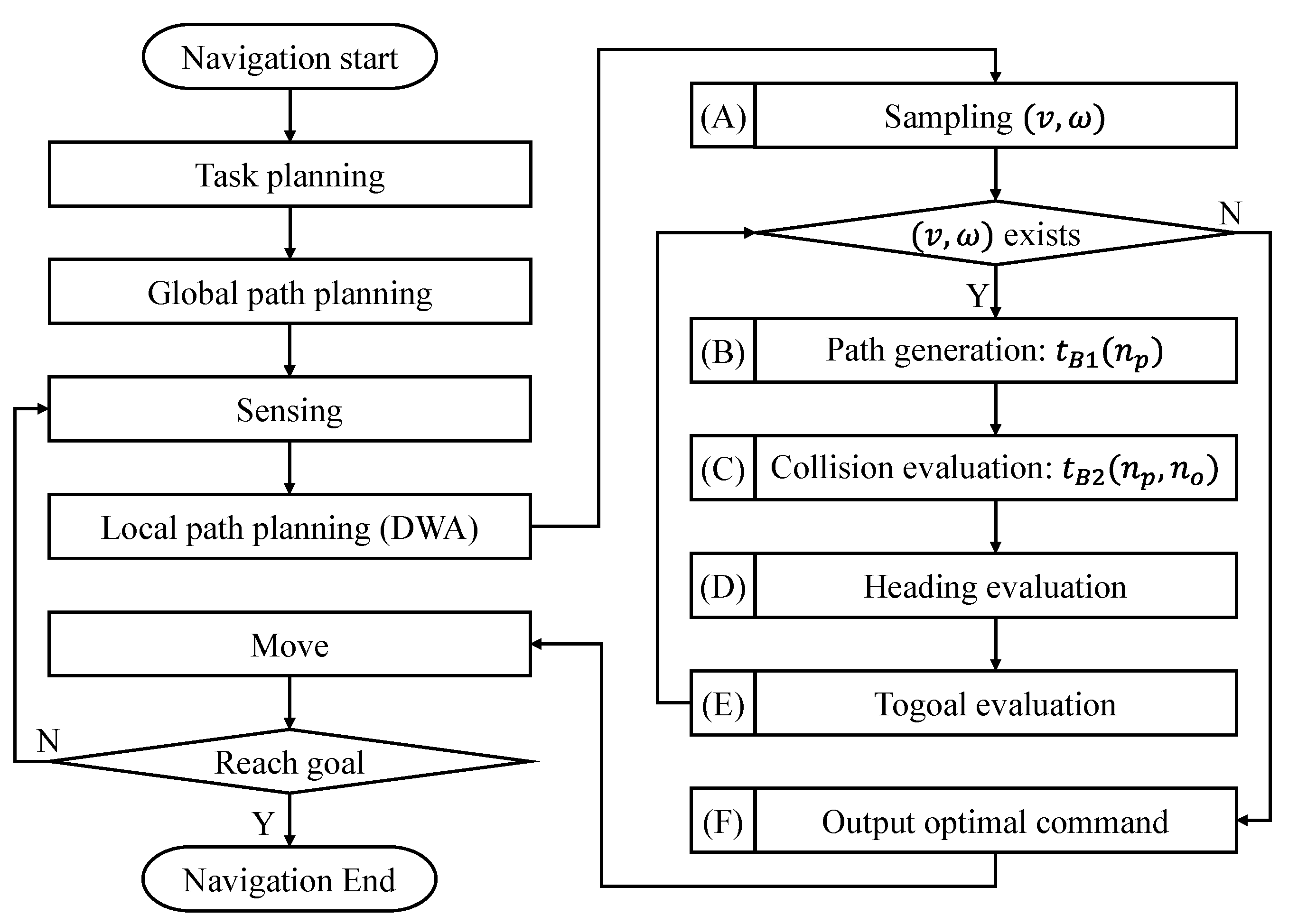
2. Dynamic Window Approach

The DWA is a local path planning algorithm in which the path is planned based on the kinematic parameters of a robot. Because the object of study is a robot that moves solely in a plane, $x\left(t\right)$, $y\left(t\right)$, and $\mathsf{\theta }\left(t\right)$ describe the configuration space of the robot, where $x\left(t\right)$ and $y\left(t\right)$ denote the coordinates, and $\mathsf{\theta }\left(t\right)$ represents the heading of the robot. Because wheeled robots that move in a plane have two degrees of freedom, translational and rotational velocities, let $v\left(t\right)$ and $\mathsf{\omega }\left(t\right)$ denote the translational and rotational velocities of the robot. The kinematic model is defined by (1)–(3).

$$x\left(t_p\right)=x\left(t_0\right)+{\int }_{t_0}^{t_p}v\left(t\right)\cdot \cos \left(\theta \left(t\right)\right)dt,$$

(1)

$$y\left(t_p\right)=y\left(t_0\right)+{\int }_{t_0}^{t_p}v\left(t\right)\cdot \sin \left(\theta \left(t\right)\right)dt,$$

(2)

$$\theta \left(t_p\right)=\theta \left(t_0\right)+{\int }_{t_0}^{t_p}\omega \left(t\right)dt.$$

(3)

For practical applications, Fox et al. presented the discrete forms of (1)–(3) expressed in (4)–(6). This model assumes that the robot moves a distance of $v·∆t$ along the heading of $t_{p-1}$, and then rotates an angle of $\omega ·∆t$. This method computes the coordinates and heading of the robot from time $t_0$ to $t_p$ by iterating the input velocities. A series of coordinates corresponding to a series of input velocities is known as a path. This model is widely employed in related studies of wheeled robots [22,23,24,25,26].

$$x\left(t_p\right)=x\left(t_{p-1}\right)+v\cdot \Delta t\cdot \cos \left(\theta \left(t_{p-1}\right)\right),$$

(4)

$$y\left(t_p\right)=y\left(t_{p-1}\right)+v\cdot \Delta t\cdot \sin \left(\theta \left(t_{p-1}\right)\right),$$

(5)

$$\theta \left(t_p\right)=\theta \left(t_{p-1}\right)+\omega \cdot \Delta t.$$

(6)

Other models predict a path from the input velocity. Equation (7)–(9) represent another kinematic model that assumes that the robot first rotates an angle of $\omega ·∆t$, and then moves a distance of $v·∆t$ along the heading of $t_p$. Yang et al. adopt this model in their work and added a factor of $\omega \cdot \Delta t$ to reduce the error in path simulation [27].

$$\theta \left(t_p\right)=\theta \left(t_{p-1}\right)+\omega \cdot \Delta t,$$

(7)

$$x\left(t_p\right)=x\left(t_{p-1}\right)+v\cdot \Delta t\cdot \cos \left(\theta \left(t_p\right)\right),$$

(8)

$$y\left(t_p\right)=y\left(t_{p-1}\right)+v\cdot \Delta t\cdot \sin \left(\theta \left(t_p\right)\right).$$

(9)

In this study, we refer to the models in (4)–(6) as tangent models and the models in (7)–(9) as secant models.

Given the absence of restrictions on velocity variation, both kinematic models yield a multitude of potential paths. In response to this, Fox et al. introduced a DWA that designates the current moment as $t_0$ and simulates the robot’s future path over a specified period by iterating (4)–(6). The conclusion of this simulation is marked as $t_p$, a timespan also referred to as the simulation period. The DWA posited that velocities remained constant throughout this simulation period. Consequently, a singular path is generated for each set of input pairs of translational and rotational velocities. These velocities were determined based on the robot’s current velocity and acceleration constraints, resulting in the number of generated paths being equivalent to the product of the translational and rotational velocities.

Figure 1 depicts a flowchart detailing the general process of robot navigation and provides an in-depth explanation of the operational mechanics of the conventional DWA. In robot navigation, the sequence initiates with the task planner setting one or multiple objectives. Following this, the global path planner is responsible for formulating the global path. Throughout the execution phase, the robot persistently scans its surrounding milieu, strategizes local trajectories, and advances, iterating this sequence until the destination is attained. The symbols 'Y' and 'N' in the flowchart represent 'Yes' and 'No,' respectively. Within the framework of the conventional DWA, the initial step, Step (A), involves the sampling of all feasible velocity pairs, grounded on the existing velocity and acceleration constraints of the robot. For each input velocity pair, the DWA computes the coordinates of the path points by iterating over (4)–(6) in Step (B), because the computation time of Step (B) primarily depends on the number of iterations $n_p$. where $t_{B1}\left(n_p\right)$ denotes the computational time for Step (B). The relationship between the number of iterations $n_p$, time interval $\mathsf{\Delta }t$, and simulation period $t_p$ can be expressed as

$$t_p=n_p\cdot \Delta t.$$

(10)

In Step (C), the DWA computes the distance between each obstacle and path point. This step can be efficiently performed using matrix operations to determine the minimum distance. The computation time for Step (C) depends on the number of paths and obstacle points. Therefore, we adopt $t_{B2}\left(n_p,n_o\right)$ to denote the computation time of Step (C). $n_o$ denotes number of obstacles. The maximum value of $n_o$ depends on the resolution and range of the sensor that detects obstacles, such as a laser rangefinder. In Steps (D) and (E), the DWA only computes the heading of the ending point of the path and the distance to the goal; hence, the computation time is extremely short and can be disregarded. After evaluating all executable velocity pairs, we output the optimal velocity command in Step (F). Therefore, the computation time of the conventional DWA, which is the baseline in this study, can be expressed as

$$t_B\left(n_p,n_o\right)=t_{B1}\left(n_p\right)+t_{B2}\left(n_p,n_o\right).$$

(11)

3. Proposed Method

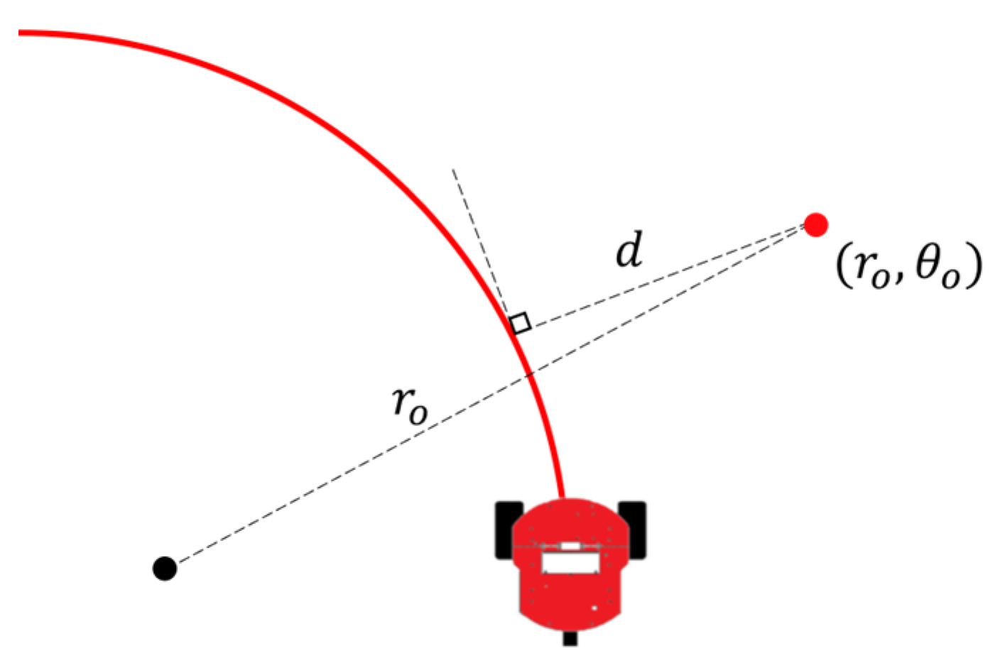
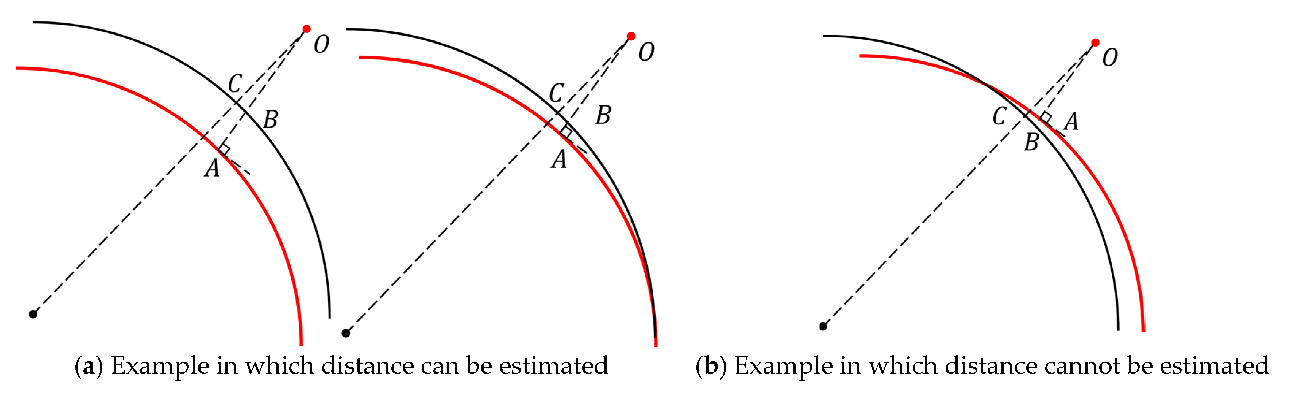
3.1. Proposed Method for Constant Velocity Model

In the conventional DWA, the robot’s velocity is presumed to remain invariant following the initial time interval. As a result, throughout the simulation period, the robot’s motion is characterized by constant velocity circular motion, rendering the simulation path as a circular arc. The relationship among translational velocity, rotational velocity, and path radius is articulated in (12) [28,29,30,31,32].

$$v=\omega \cdot r_p,$$

(12)

where $v$ and $\mathsf{\omega }$ represent the translational and rotational velocities of a robot during the simulation period, respectively, $r_p$ denotes the radius of simulation path.

Accordingly, we can establish a polar coordinate system with the center of the circular arc path ($x_p,y_p$) as the origin. Subsequently, we can convert the coordinates of obstacles in the robot coordinate system ($x_o,y_o$) to the polar coordinate system ($r_o,{\theta }_o$) using (13) and (14). The function atan2 was adopted to calculate the angle after coordinate transformation.

$$r_o=\sqrt{{\left(x_o-x_p\right)}^2+{\left(y_o-y_p\right)}^2},$$

(13)

$${\theta }_o=\mathrm{a}\mathrm{t}\mathrm{a}\mathrm{n}2\left(y_o-y_p,x_o-x_p\right).$$

(14)

Finally, we can employ the radial coordinates of the obstacles $r_o$ and path radius $r_p$ to compute the distance from the obstacles to the simulation path using (15).

$$d=\left|r_o-r_p\right|.$$

(15)

Figure 2a illustrates this process. ($x_o,y_o$) represents the coordinates of an obstacle, and ($x_p,y_p$) denotes the center of the circular arc path in the robot coordinate system. As illustrated in Figure 2b, the coordinate of the obstacle is ($r_o,{\theta }_o$) after conversion. Next, the distances from the circular arc path to all obstacle points are computed. When the minimum value of the distance is smaller than the safe distance, the algorithm abandons the simulation path.

A flowchart of the proposed method is presented in Figure 3. In contrast to the conventional DWA, the proposed method does not require the generation of discrete path points, which enables it to omit iterative computations in time. The symbols 'Y' and 'N' in the flowchart represent 'Yes' and 'No,' respectively. In Step (B), the coordinates of the polar origins are computed as denoted by $t_{P1}\left(n_c\right)$, where $n_c$ represents the number of polar origins. When generating paths using the constant velocity model, $n_c$ can be viewed as a constant of 1. In step (C), the proposed method performs polar transformations on all obstacle points; hence, the computation time of Step (C) depends on the number of polar origins $n_c$ and obstacle points $n_o$. Therefore, we utilize $t_{P2}\left(n_c,n_o\right)$ to denote the computation time of Step (C). The total computation time of the proposed method is expressed as (16). Because $n_c$ is significantly smaller than $n_p$, we presume that the computation time of the proposed method is shorter than that of the conventional DWA.

$$t_P\left(n_c,n_o\right)=t_{P1}\left(n_c\right)+t_{P2}\left(n_c,n_o\right).$$

(16)

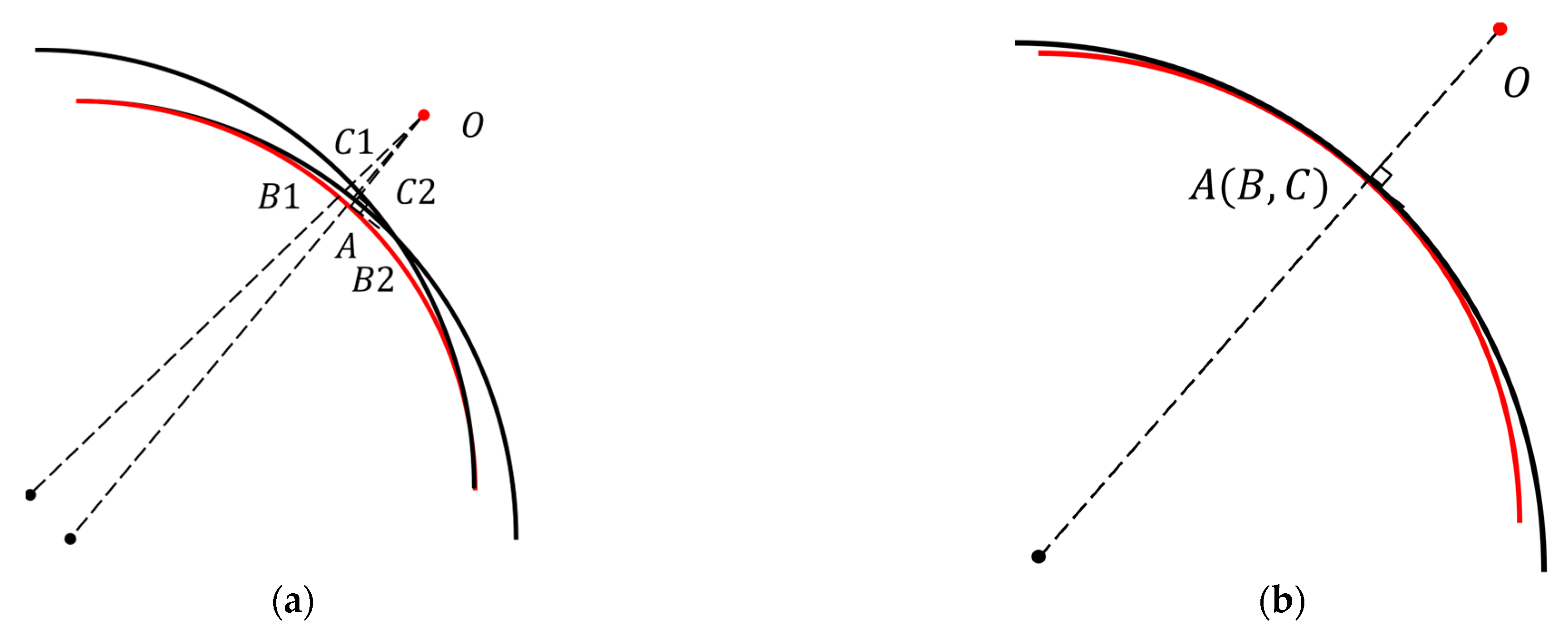
3.2. Proposed Method for the Variable Velocity Model

When the method proposed in [17] is adopted to generate variable velocity paths, the circular arc paths become curved with monotonically increasing and decreasing curvatures, as illustrated in Figure 4. The black line represents a circular arc path. The red and blue lines represent the paths during acceleration and deceleration, respectively. The curvature of the path continued to increase in the case of acceleration and decreased in the case of deceleration. $v_0$ and ${\mathsf{\omega }}_0$ denote the robot’s initial translational and rotational velocities, respectively, and $v_p$ denotes the terminal translational velocity. The curvature of the path is $\frac{v_0}{{\omega }_0}$ at time $t_0$, and $\frac{v_p}{{\omega }_0}$ at time $t_p$.

As depicted in Figure 5, the perpendicular line drawn from the obstacles to the path does not consistently run parallel to the line extending from the obstacles to the origin of the polar coordinate system. Consequently, the distance from the obstacles to the path cannot be calculated using (15). In light of this, the present paper introduces a method to infer the distance from obstacles to a path, employing multiple polar coordinate transformations. This method is applicable to paths with monotonically increasing or decreasing curvatures.

Figure 6 presents an example of a path generated by the acceleration model. The side where the center of curvature resides is referred to as the inner side, and the opposing side is termed the outer side. Initially, we established a polar coordinate system, designating any point on the inner side of the path as the origin, and subsequently drew a circle centered at this origin. This circle may either be separate from, tangential to, or intersecting with the path.

The line from the obstacles to the center of the circle intersects the circle and path at Points C and B, respectively. The foot of the perpendicular line from the obstacles to the path is called Point A. Owing to the length of OA being the shortest distance from the obstacles to the path, OA ≤ OB. As illustrated in Figure 6a, when the circle is separated from or tangential to the path, OB ≤ OC; hence, OA ≤ OC. As illustrated in Figure 6b, when the circle intersects the path, we cannot determine the size relationship between OA and OC owing to the location of the obstacles. Thus, we can establish a size relationship between OA and OC if the circle does not intersect with the path.

Furthermore, the larger the radius of the circle, the smaller OC is, and the closer it is to OA. To improve the distance estimation accuracy, the largest circle that does not intersect the path should be adopted. Because the path’s range of curvature is $\left[\frac{v_0}{{\omega }_0},\frac{v_p}{{\omega }_0}\right]$, the largest radius of the circle is $\frac{v_0}{{\omega }_0}$.

As illustrated in Figure 7a, multiple circles were generated on the inner side. As aforementioned, OA ≤ min(OC1, OC2). This implies that as more circles are generated, the probability that min(OC1, OC2, …) is close to that of OA increases. If, and only if, Point A is the contact point of the circle and path, as illustrated in Figure 7b, Points A, B, and C coincide to form a single point, and the equality sign in the inequality OA ≤ OC holds, then the proposed method can compute the true value of OA accurately.

At this point, the boundary on one side of the distance from the obstacle to the path is determined. Similarly, the circle can be separated from, tangential to, or intersecting with the path on the outer side, as illustrated in Figure 8. The line from the obstacles to the center of the circle intersects with the circle at Point C. The foot of the perpendicular line from the obstacles to the path is called Point A, and the perpendicular line intersects with the circle at Point B. Because the length of OA is the shortest distance from the obstacles to the path, OB ≤ OA. As illustrated in Figure 8a, when the circle is separated from or tangential to the path, OC ≤ OB; hence, we can deduce that OC ≤ OA. As illustrated in Figure 8b, when the circle intersects with the path, we cannot determine the size relationship between OA and OC owing to the location of the obstacles. Based on the above discussion, it is evident that we can establish a size relationship between OA and OC if the circle does not intersect with the path.

Moreover, the smaller the radius of the circle, the larger OC is and the closer it is to OA. To improve the accuracy of distance estimation, the smallest circle that does not intersect the path should be employed. Because the path’s range of curvature is $\left[\frac{v_0}{{\omega }_0},\frac{v_p}{{\omega }_0}\right]$, the smallest radius of the circle is $\frac{v_p}{{\omega }_0}$.

As illustrated in Figure 9a, multiple circles were generated on the outer side. As mentioned above, the more circles generated on the outer side, the higher the probability that max(OC1, OC2) is close to that of OA. If, and only if, Point A is the contact point between the circle and path, as illustrated in Figure 9b, Points A, B, and C converge into one, and the equality sign in the inequality OC ≤ OA holds. In this case, the proposed method could accurately compute the true OA value. By combining the distance estimations from both sides, the range of the distance from the obstacle to the path can be obtained. Because multiple circles are generated on the inner and outer sides of the path, $n_c$ in (16) is no longer unity. Nonetheless, $n_c$ is still much smaller than $n_p$, so a shorter computation time can be expected for the proposed method compared to that for the conventional DWA.

3.3. Computations

According to [17], by replacing the constant translational velocity sequence in the conventional DWA with a variable translational velocity sequence, a larger range of path reach points can be achieved. As illustrated in Figure 10, under the conditions of a robot’s initial velocity of (1.0, 0.0), maximum translational velocity of 2.0 $\left[\frac{\mathrm{m}}{\mathrm{s}}\right]$, and maximum acceleration of 1.0 $\left[\mathrm{m}/{\mathrm{s}}^2\right]$, we compare the predicted range of path waypoints for the conventional DWA, constant translational acceleration model, and constant translational jerk model at prediction times of 0.8 and 2.0 $\left[s\right]$. The acceleration model exhibits a larger range of reaching points. Here, we adopt the acceleration model as a variable velocity model, as defined in (17) and (18).

$$v\left(t\right)=\left\{\begin{array}{c}{v}_0+a\cdot t 0\le t\le t_{ea}\mid or\mid 0\le t\le t_{ed}\\ v_{max} t_{ea}<t\le t_p\mid and\mid a>0\\ 0 t_{ed}<t\le t_p\mid and\mid a\le 0\end{array}\right.,$$

(17)

$$\omega \left(t\right)={\omega }_0.$$

(18)

This model assumes that translational acceleration and rotational velocity remain constant between time $t_0$ and $t_p$. $v_0$ denotes the initial translational velocity of the robot, $v_{max}$ denotes the maximum translational velocity, $a$ represents the selected acceleration ($a\in \left[-a_{max},a_{max}\right]$), and $t_p$ is the simulation period. For simplicity, we denote $\frac{v_{max}-v_0}{a}$ as $t_{ea}$ and $\frac{v_0}{a}$ as $t_{ed}$.

With the acceleration case as an example, we substitute (17) and (18) into (1)–(3) and use $v^{\prime }\left(t\right)$ and ${\theta }^{\prime }\left(t\right)$ in place of $v_0+a\cdot t$ and $\theta \left(t_0\right)+{\omega }_0\cdot t$; consequently, (19), (20), (21) are obtained.

$$x_{path}\left(t\right)=\left\{\begin{array}{c}\frac{{\omega }_0\cdot v^{\prime }\left(t\right)\mathit{sin}\left({\theta }^{\prime }\left(t\right)\right)+a\cdot \cos \left({\theta }^{\prime }\left(t\right)\right)}{{{\omega }_0}^2}+c_1\\ \frac{v_{max}}{{\omega }_0}\sin \left({\theta }^{\prime }\left(t\right)\right)+c_2\end{array}\right.,$$

(19)

$$y_{path}\left(t\right)=\left\{\begin{array}{c}\frac{-{\omega }_0\cdot v^{\prime }\left(t\right)\mathit{cos}\left({\theta }^{\prime }\left(t\right)\right)+a\cdot \sin \left({\theta }^{\prime }\left(t\right)\right)}{{{\omega }_0}^2}+c_3\\ -\frac{v_{max}}{{\omega }_0}\cos \left({\theta }^{\prime }\left(t\right)\right)+c_4\end{array}\right.,$$

(20)

$${\theta }_{path}\left(t\right)={\omega }_0\cdot t.$$

(21)

Next, we simplify the first interval of (19) as $A\left(t\right)+c_1$, the second interval as $B\left(t\right)+c_2$, first interval of (20) as $C\left(t\right)+c_3$, and the second interval as $D\left(t\right)+c_4$. Finally, we compute the constant of integration using Equations (22)–(25).

$$\underset{t\to 0^{+}}{\mathit{lim}}A\left(t\right)+c_1=0,$$

(22)

$$\underset{t\to 0^{+}}{\mathit{lim}}C\left(t\right)+c_3=0,$$

(23)

$$\underset{t\to {t_{\mathit{ea}}}^{-}}{\mathit{lim}}A\left(t\right)+c_1=\underset{t\to {t_{\mathit{ea}}}^{+}}{\mathit{lim}}B\left(t\right)+c_2,$$

(24)

$$\underset{t\to {t_{\mathit{ed}}}^{-}}{\mathit{lim}}C\left(t\right)+c_3=\underset{t\to {t_{\mathit{ed}}}^{+}}{\mathit{lim}}D\left(t\right)+c_4.$$

(25)

Subsequently, the position of the center must be determined because the radius of the circle has been determined. First, we generate a pair of circles in contact with the starting point of the path. The function of the inner circle is defined in (26) and (27), and that of the outer circle is expressed in (28) and (29). The center points of the circles are $\left(0,\frac{v_0}{{\omega }_0}\right)$ and $\left(0,\frac{v_p}{{\omega }_0}\right)$, respectively.

$$x_{ic}\left(t\right)=\frac{v_0}{{\mathsf{\omega }}_0}\sin \left({\mathsf{\omega }}_0\cdot t\right),$$

(26)

$$y_{ic}\left(t\right)=\frac{v_0}{{\mathsf{\omega }}_0}\left(1-\cos \left({\mathsf{\omega }}_0\cdot t\right)\right),$$

(27)

$$x_{oc}\left(t\right)=\frac{v_p}{{\mathsf{\omega }}_0}\sin \left({\mathsf{\omega }}_0\cdot t\right),$$

(28)

$$y_{oc}\left(t\right)=\frac{v_p}{{\mathsf{\omega }}_0}\left(1-\cos \left({\mathsf{\omega }}_0\cdot t\right)\right).$$

(29)

The other circles can be considered as the translation of this pair of circles, and the magnitudes of the translation are computed using (30)–(33). Hence, the centers of other circles are $\left(0-\Delta x_{ic}\left(t\right),\frac{v_0}{{\omega }_0}-\Delta y_{ic}\left(t\right)\right)$ and $\left(0-\Delta x_{oc}\left(t\right),\frac{v_p}{{\omega }_0}-\Delta y_{oc}\left(t\right)\right)$.

$$\Delta x_{ic}\left(t\right)=x_{ic}\left(t\right)-x_{path}\left(t\right),$$

(30)

$$\Delta y_{ic}\left(t\right)=y_{ic}\left(t\right)-y_{path}\left(t\right),$$

(31)

$$\Delta x_{oc}\left(t\right)=x_{oc}\left(t\right)-x_{path}\left(t\right),$$

(32)

$$\Delta y_{oc}\left(t\right)=y_{oc}\left(t\right)-y_{path}\left(t\right).$$

(33)

An example of the generation of two pairs of circles is shown in Figure 11. In this example, the starting and ending points of the path were adopted as the contact points with circles. Circles c1 and c3 are inner side, circles c2 and c4 are outer side circles. Equations (34)–(37) define the distance from obstacle $\mathrm{O}$ to the center of each circle.

$$r_{ic1}={‖\left(x_o,y_o\right)-\left(\mathsf{\Delta }{x}_{ic}\left(0\right),\mathsf{\Delta }{y}_{ic}\left(0\right)\right)‖}_2,$$

(34)

$$r_{ic2}={‖\left(x_o,y_o\right)-\left(\mathsf{\Delta }{x}_{ic}\left(t_p\right),\mathsf{\Delta }{y}_{ic}\left(t_p\right)\right)‖}_2,$$

(35)

$$r_{oc1}={‖\left(x_o,y_o\right)-\left(\mathsf{\Delta }{x}_{oc}\left(0\right),\mathsf{\Delta }{y}_{oc}\left(0\right)\right)‖}_2,$$

(36)

$$r_{oc2}={‖\left(x_o,y_o\right)-\left(\mathsf{\Delta }{x}_{oc}\left(t_p\right),\mathsf{\Delta }{y}_{oc}\left(t_p\right)\right)‖}_2.$$

(37)

The distance $d$ from the obstacle to the path is expressed by (38).

$$\max \left(r_{oc1}-\frac{v_p}{v_0},r_{oc2}-\frac{v_p}{v_0}\right)\le d\le \mathrm{m}\mathrm{i}\mathrm{n}\left(r_{ic1}-\frac{v_0}{v_0},r_{ic2}-\frac{v_0}{v_0}\right).$$

(38)

However, additional steps are required for practical applications. As illustrated in Figure 12, a polar coordinate system centered on the intersection of the normals of the starting point (A) and ending point (B) of the path was created. Two normal lines divide the plane into four regions. The polar angle of the obstacle was then adopted to determine the four areas to which it belonged. For obstacles such as $O1$ and $O4$ in the grey area, the distance to the path is the minimum distance from the start and end of the path. For obstacles such as $O2$ and $O3$ in the white area, the proposed method determines the range of distances, and the middle value of the range is adopted as the distance.

4. Experiment

When generating paths using the constant velocity model within the conventional DWA, all paths are circular arcs. Therefore, when applying the proposed method, only one transformation is required, with $n_c$ set to 1. Hence, the proposed method necessitates only a single path through all obstacle points to compute distances, contrasting with the conventional DWA which requires traversing both obstacle and path points. This results in a noteworthy advantage in computational time for the proposed method.

Furthermore, as illustrated in Figure 2, the proposed method reliably calculated the true distance values. In the conventional DWA, predicted paths are represented through discrete path points, and collision detection is executed by determining the minimum distance between the sets of path and obstacle points. A lower number of path points can result in substantial errors in collision detection, thereby highlighting a significant accuracy advantage of the proposed method.

Given that the proposed method demonstrated both swifter computation time and enhanced accuracy compared to the conventional DWA employing the constant velocity model, we restricted our assessment to the efficacy of the proposed method when generating paths using the more intricate acceleration model.

The experimental environment and control program were constructed utilizing the Robot Operating System (ROS) [33]. In these experiments, a two-dimensional simulator named Stage [34] was adopted, given the robot’s movement was confined to a plane. Due to the extensive computation time needed to ascertain the true distance values from the obstacle points to the path, it was impractical to concurrently compute the accuracy of distance calculation and computation time of the two methods in the navigation experiment. Consequently, two distinct experiments were conducted. In the initial experiment, the accuracy of distance calculation of the two methods was compared, with the robot stationary and only predicting the path.

In the second experiment, the computation time for each method during navigation was measured.

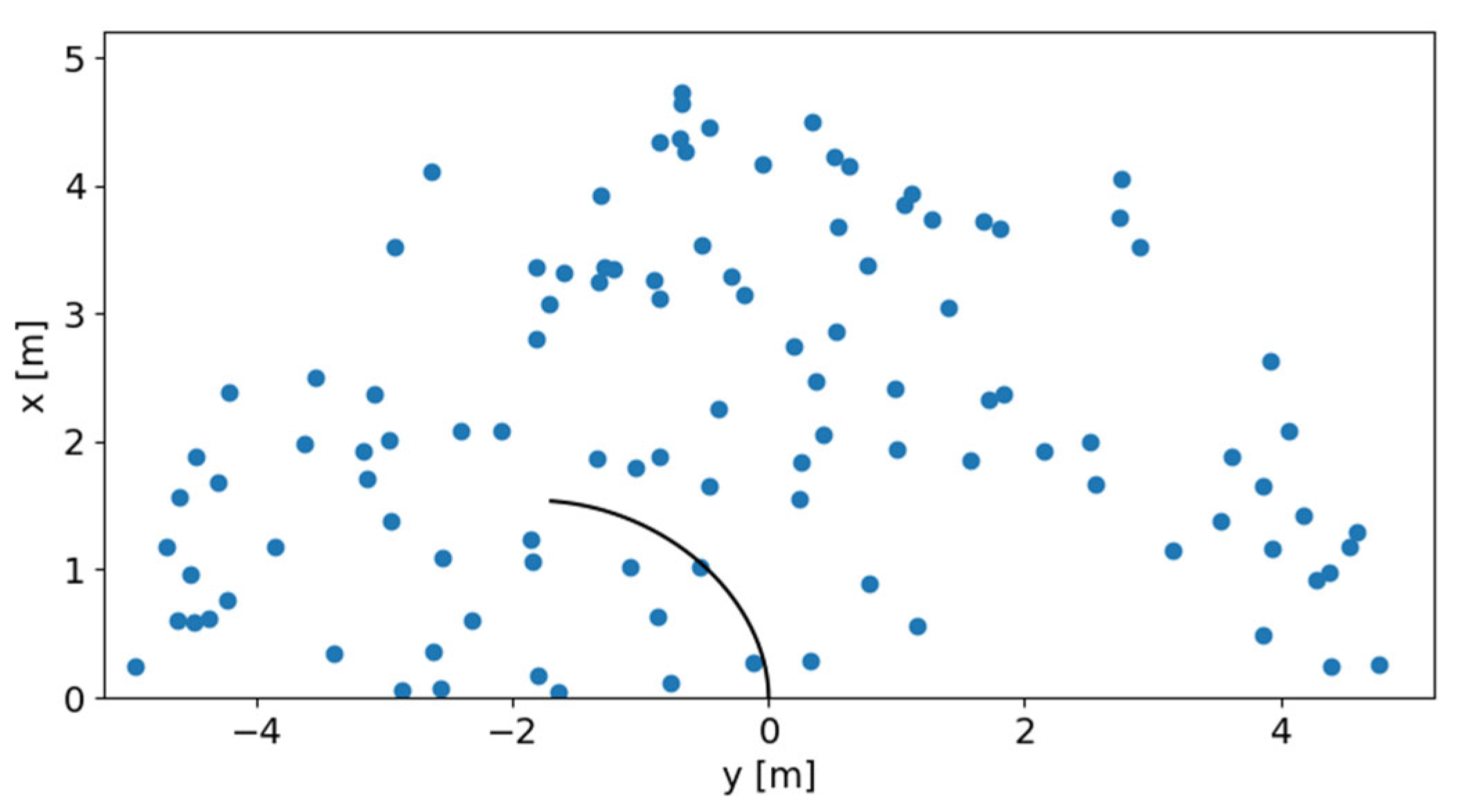
4.1. Conditions of Distance Calculation Accuracy Experiment

Figure 13 illustrates the environment of the first experiment. The initial position of the robot is set to (0, 0), and the black line represents the simulation path. We randomly generated 100 points within a circular area in front of the robot to simulate the obstacles. The radius of the circular area was 5 $\left[\mathrm{m}\right]$, which was consistent with the detection distance of the laser rangefinder. The simulation period $t_p$ was set to 2.0 $\left[\mathrm{s}\right]$. The translational and rotational velocities were set to 1.0 [$\mathrm{m}/\mathrm{s}$] and 1.0 $\left[\mathrm{r}\mathrm{a}\mathrm{d}/\mathrm{s}\right]$, respectively. The translational acceleration in the simulation period was set to −1.0, −0.5, 0.0, 1.0, 0.5 $\left[\mathrm{m}/{\mathrm{s}}^2\right]$.

The number of circles in the proposed method was set to 1, 2, and 3 pairs; hence, $n_c$ values were 2, 4, and 6. The generated circle contacted the start, middle, and end points of the simulation path. In this study, we consider only the case in which a pair of circles is generated at the same tangent point; therefore, when $n_c$ is 2, there are three cases of tangent points at the starting (s), middle (m), and ending points of the path. When $n_c$ is 4, there are three cases of tangent points at the starting and middle (s + m), starting and ending (s + e), and middle and ending (m + e) points of the path. When $n_c$ = 6, only one tangent point exists at the starting, middle, and ending (s + m + e) points of the path.

For the conventional DWA, the time interval $∆t$ is set to 0.10, 0.05, 0.02 [s]; hence, $n_p$ values are 20, 40, and 100, respectively.

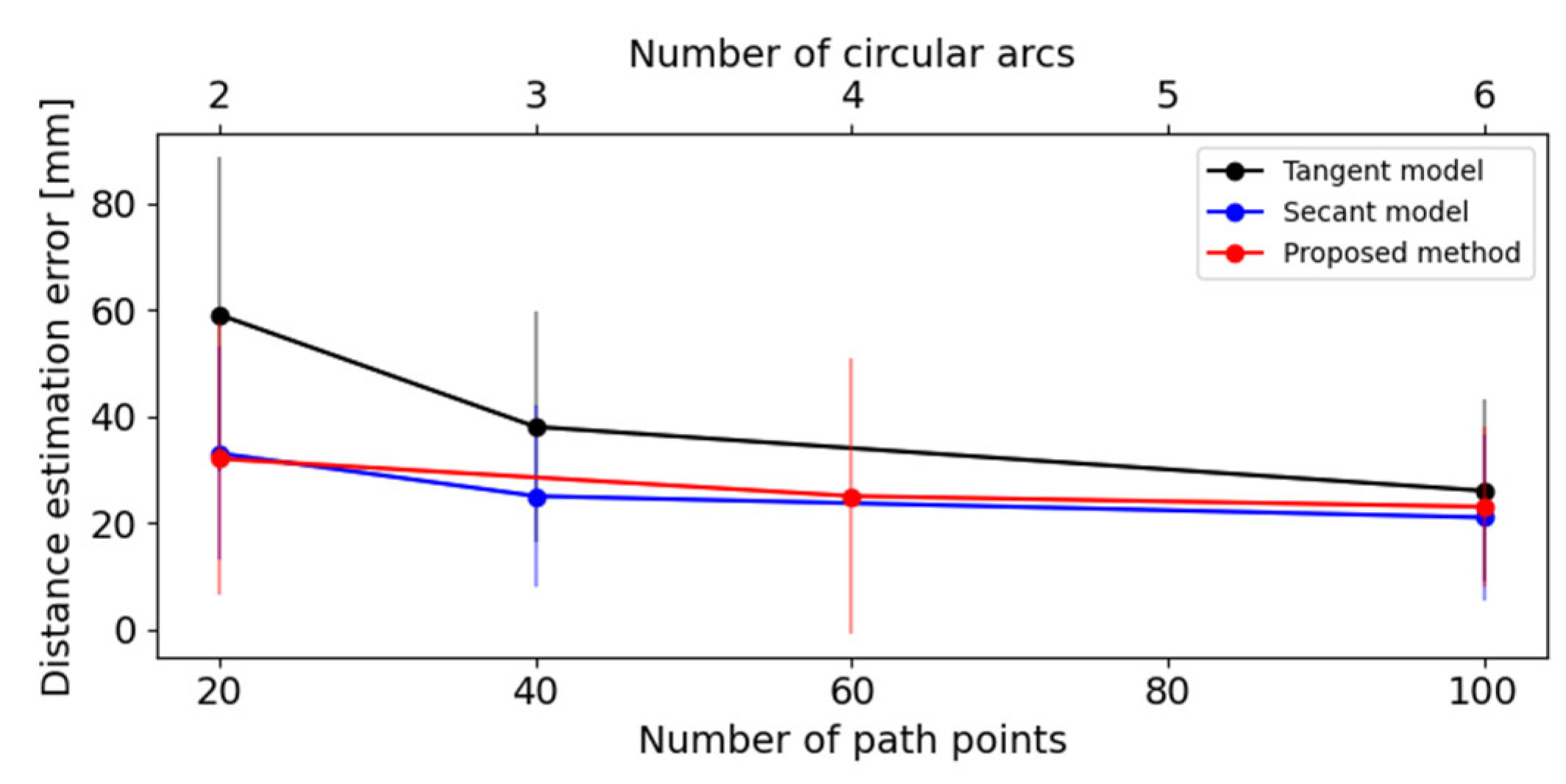
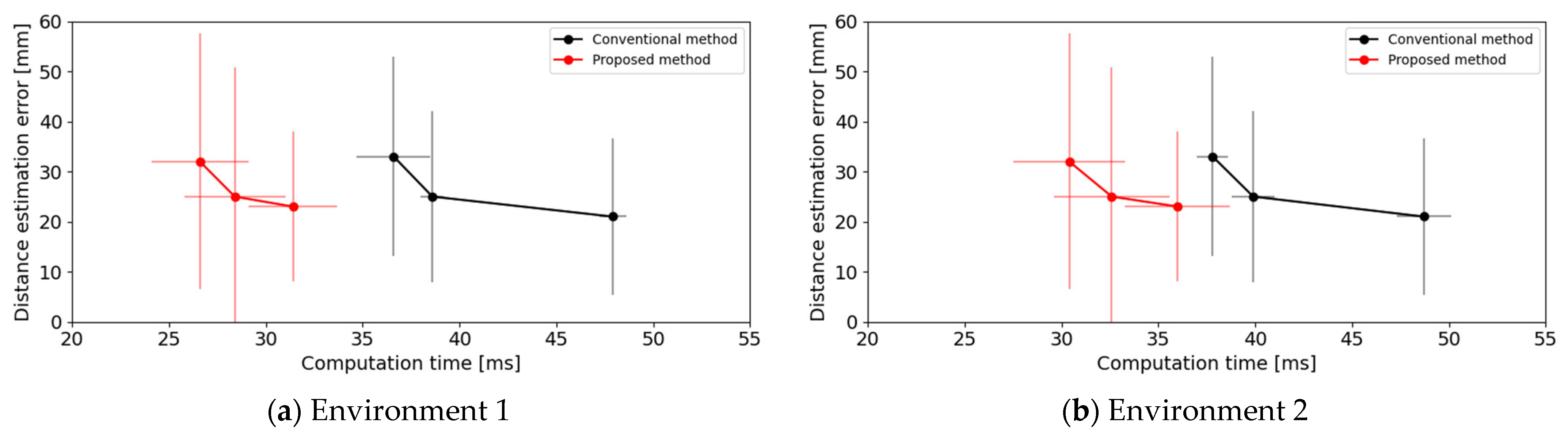
4.2. Results of Distance Calculation Accuracy Experiment

We computed the distance from each obstacle to the path using analytic geometry as the baseline. The difference between the distance obtained by the proposed method and the baseline was used as the error, and we adopted the average value of the errors to evaluate the performance of the distance estimation.

Table 1. Average error of distance estimation under proposed method.

Trans acc.	${\mathit{n}}_{\mathit{c}}=2$			${\mathit{n}}_{\mathit{c}}=4$			${\mathit{n}}_{\mathit{c}}=6$
	s	m	e	s + m	s + e	m + e	s + m + e
−1.0	34	28	181	29	30	29	31
−0.5	102	22	84	16	19	27	13
0.0	0	0	0	0	0	0	0
0.5	98	30	161	33	30	47	30
1.0	55	78	317	46	81	71	42
Mean	58	32	148	25	32	35	23
Std	38.9	25.5	105.6	15.7	27.0	23.6	14.9

presents the average error of the distance estimation in millimeters. First, as the number of circles increases, the mean of the average error in the distance estimation for each acceleration decreases. Specifically, when $n_c=2$, the circle with the tangent point at the midpoint (m) of the path better represents the trend of the entire path, resulting in a lower error. Similarly, when $n_c=4$, the circle with tangent points at the starting and middle points (s + m) of the path provides a better description of the path trend, resulting in a lower error for (s + m). Finally, when $n_c=6$, for translational accelerations ranging from −1.0 to 1.0 $\left[\mathrm{m}/{\mathrm{s}}^2\right]$, (s + m + e) has the smallest estimation error. This matches the expectation that the greater the number of circles, the smaller the distance estimation error.

Subsequently, the proposed method approximates the variable velocity path with multiple constant velocity circular paths through vertical observation. Consequently, when variations in velocities were minimal, the error in distance estimation was reduced. Specifically, when the translational acceleration during the simulation period is 0.0 $\left[\mathrm{m}/{\mathrm{s}}^2\right]$, resulting in the robot’s constant velocity circular motion, the proposed method can accurately compute the actual distance between obstacles and paths, particularly when the translational acceleration during the simulation period is nullified.

Table 2. Average error of distance estimation under conventional DWA.

Trans acc.	${\mathit{n}}_{\mathit{p}}=20$		${\mathit{n}}_{\mathit{p}}=40$		${\mathit{n}}_{\mathit{p}}=100$
	Tangent	Secant	Tangent	Secant	Tangent	Secant
−1.0	55	51	42	40	34	33
−0.5	23	18	12	9	5	4
0.0	32	1	16	1	7	1
0.5	78	39	51	32	36	28
1.0	104	52	69	43	48	38
Mean	59	33	38	25	26	21
Std	29.5	19.9	21.5	17.1	17.1	15.6

displays the average error in distance estimation, measured in millimeters. Examining horizontally, it can be observed that as the number of path points escalates, the mean of the average error in distance estimation for each acceleration diminishes under both tangent and secant models. However, a decrease in estimation error corresponds to an increase in computing cost. The accuracy of distance estimation employing the secant model consistently surpassed that of the tangent model.

When observed vertically, both the tangent and secant models demonstrate the characteristic that a reduction in translational acceleration corresponds to a decrease in distance estimation error.

We compared the distance estimation results of the best-performing configuration of the proposed method, that is, (s, s + m, s + m + e), with the tangent and secant models in the conventional DWA under various $n_p$ conditions. In Figure 14, the horizontal axis denotes the number of path points $n_p$ in the conventional DWA, the number of circular arcs $n_c$ in the proposed method, and the vertical axis denotes the average error of distance estimation. The error bars indicate the standard deviation caused by the acceleration change. The comparison shows that the proposed method achieves a similar level of accuracy in distance estimation as the secant model, which performs better in the conventional DWA.

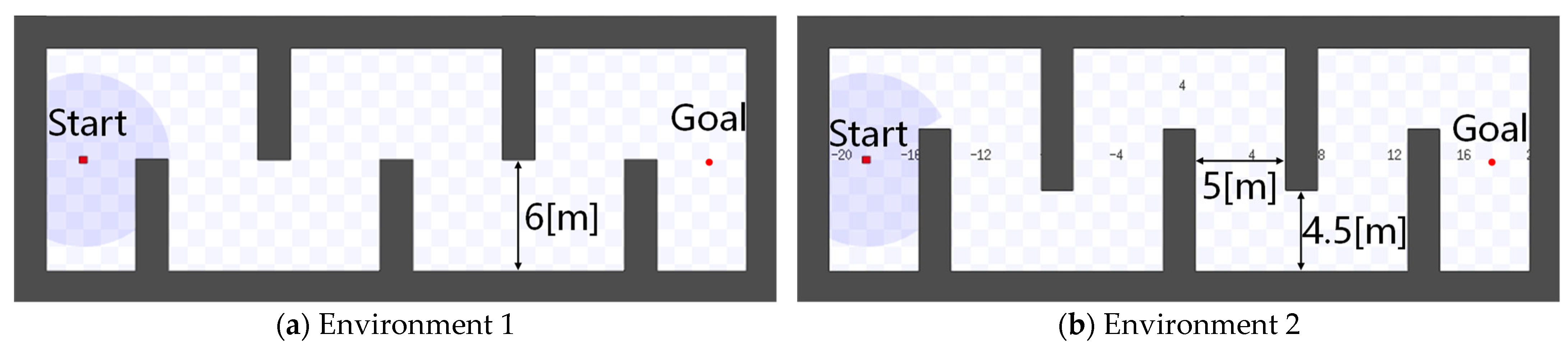
4.3. Conditions of Navigation Experiment

The second experiment was conducted to compare the performances of the two methods in terms of the computational cost of navigation.

Table 3. Parameters of experiment environment.

System Configuration	Details
OS	Ubuntu 18.04.5 LTS
ROS	Melodic 1.14.9
Stage	4.3.0
CPU	Intel Core i7-8700 3.20Ghz×12
Numpy	1.16.4
Scipy	1.3.0

lists the parameters of the PC and other libraries, and Figure 15 illustrates the experimental environment in the simulator; the environment shown in (b) is narrower than (a). The maximum velocity of the robot was set to 2.0 [$\mathrm{m}/\mathrm{s}$], maximum acceleration to 1.0 [$\mathrm{m}/{\mathrm{s}}^2$], the robot’s initial position to (−18, 0), and the target to (18, 0). The control frequency was established at 10 Hz. In this configuration, we utilized an automatic time padding technique. Should the cumulative duration consumed by all procedures within a loop fall below 100 milliseconds, the system automatically allocates the idle time to uphold a consistent control frequency of 10 Hz. The range of the laser rangefinder was set to 5 [m], and the resolution was set to 1, 2, or 3 [nums/°]. For the environment illustrated in Figure 15, the average numbers of obstacle points detected per frame during autonomous navigation $n_o$ is approximately 130, 260, and 390. We controlled the value of $n_o$ by adjusting the laser rangefinder resolution; therefore, $n_o$ is the result and is for reference only. The simulation period was set to 2 [s], and the time interval $\mathsf{\Delta }t$ of the conventional DWA was set to 1.00, 0.50, 0.20, 0.10, 0.05, 0.02 [s], according to (7); $n_p$ values are 2, 4, 10, 20, 40, and 100, respectively. The number of circles in the proposed method was set to 1, 2, and 3 pairs; hence, $n_c$ values were 2, 4, and 6. Both the conventional DWA and proposed method divide the selectable translational acceleration and rotational velocity ranges into five equal parts, generating 25 simulation paths simultaneously. Ten automatic navigations were performed in the simulation environment and the average computation time of the DWA was determined in milliseconds. Since all navigation experiments in both environments were successful only for $n_p>20$, using the results obtained with $n_p=20$ and $n_c=2$ as the baseline, we attempted to determine whether there was a significant change in the calculation time when $n_p$ and $n_c$ were varied. We adopted * to indicate p-values less than 0.05 and ** to indicate p-values less than 0.01.

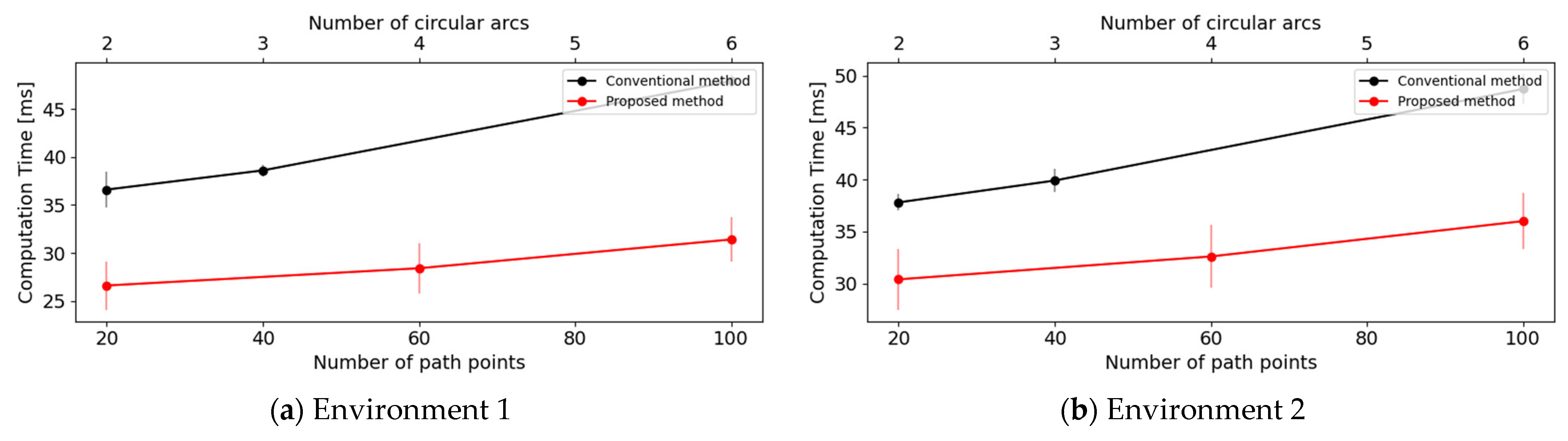
4.4. Results of Navigation Experiment

Comparison of the travel distance and time is shown in

Table 4. Travel distance and time of conventional DWA and proposed method in Environment 1.

Laser Rangefinder Resolution [nums/°]		1		2		3
Number of Detected Obstacle Points per Frame		${\mathit{n}}_{\mathit{o}}\approx 130$		${\mathit{n}}_{\mathit{o}}\approx 260$		${\mathit{n}}_{\mathit{o}}\approx 390$
		Travel Distance [m]	Travel Time [s]	Travel Distance [m]	Travel Time [s]	Travel Distance [m]	Travel Time [s]
Conventional DWA	$n_p=2$	90.6	79.9	90.4	79.9	89.4	79.9
	$n_p=4$	44.8	26.7	44.4	26.5	43.0	25.5
	$n_p=10$	39.2	23.4	39.4	23.1	39.0	23.5
	$n_p=20$	39.0	23.6	39.2	23.5	39.2	23.6
	$n_p=40$	39.0	25.0	39.0	25.2	39.0	25.0
	$n_p=100$	39.0	24.8	39.0	25.0	39.6	23.6
Proposed method	$n_c=2$	38.4	21.5	38.4	21.6	38.4	21.5
	$n_c=4$	38.4	21.6	38.0	21.3	38.1	21.4
	$n_c=6$	39.1	25.1	39.0	24.9	39.1	25.0

and

Table 5. Travel distance and time of conventional DWA and proposed method in Environment 2.

Laser Rangefinder Resolution [nums/°]		1		2		3
Number of Detected Obstacle Points per Frame		${\mathit{n}}_{\mathit{o}}\approx 130$		${\mathit{n}}_{\mathit{o}}\approx 260$		${\mathit{n}}_{\mathit{o}}\approx 390$
		Travel Distance [m]	Travel Time [s]	Travel Distance [m]	Travel Time [s]	Travel Distance [m]	Travel Time [s]
Conventional DWA	$n_p=2$	86.0	79.9	85.2	79.9	87.6	79.9
	$n_p=4$	66.2	52.7	63.4	46.8	61.2	42.9
	$n_p=10$	60.8	42.5	61.2	41.6	61.2	41.5
	$n_p=20$	53.4	30.7	53.6	31.4	53.8	30.9
	$n_p=40$	53.6	32.1	53.2	32.5	53.6	32.2
	$n_p=100$	55.8	31.7	56.0	31.8	55.6	31.5
Proposed method	$n_c=2$	51.6	30.5	54.3	31.6	52.6	31.1
	$n_c=4$	53.1	31.4	54.4	32.2	53.6	31.7
	$n_c=6$	53.6	31.7	54.1	32.0	54.3	32.1

. In the experimental setup, the straight-line distance between the initial position and the target is 36 [m]. The results in Table 4 indicate a significant difference in travel distance and other results for $n_p<10$. This is attributed to the sparse distribution of path points, causing the robot to lose its way during autonomous navigation. Since Environment 2 is narrower than Environment 1, examining the results in

Table 6. Computing time of conventional DWA and proposed method in Environment 1.

Laser Rangefinder Resolution [nums/°]		1		2		3
Number of Detected Obstacle Points per Frame		${\mathit{n}}_{\mathit{o}}\approx 130$		${\mathit{n}}_{\mathit{o}}\approx 260$		${\mathit{n}}_{\mathit{o}}\approx 390$
		Mean	p	Mean	p	Mean	p
Conventional DWA	$n_p=2$	16.1	-	20.6	-	24.0	-
	$n_p=4$	17.8	-	21.3	-	23.8	-
	$n_p=10$	25.4	-	30.9	-	32.9	-
	$n_p=20$	34.6	-	36.1	-	39.1	-
	$n_p=40$	37.8	*	38.7	*	39.3
	$n_p=100$	47.3	**	47.5	**	48.8	**
Proposed method	$n_c=2$	24.7	-	25.0	-	30.1	-
	$n_c=4$	25.1		28.7		31.5
	$n_c=6$	29.4	*	30.2		34.7

* to indicate p-values less than 0.05 and ** to indicate p-values less than 0.01.

, when $n_p$ is less than 20, successful navigation becomes challenging. Hence, for more complex environments, robots require more path points for successful navigation.

When there are enough path points to guarantee successful navigation, one might observe that there is no substantial disparity in the navigation travel distance and time between the conventional DWA and our proposed method. This similarity arises because the experiments were conducted at an identical control frequency. In real-world robotic operations, each control loop encompasses not just local path planning, but also tasks of environmental perception and specific task processing, such as real-time image processing. Hence, curtailing the time spent on local path planning affords additional time for other crucial operations.

A comparison of the computing time per frame is shown in Table 6 and

Table 7. Computing time of conventional DWA and proposed method in Environment 2.

Laser Rangefinder Resolution [nums/°]		1		2		3
Number of Detected Obstacle Points per Frame		${\mathit{n}}_{\mathit{o}}\approx 130$		${\mathit{n}}_{\mathit{o}}\approx 260$		${\mathit{n}}_{\mathit{o}}\approx 390$
		Mean	p	Mean	p	Mean	p
Conventional DWA	$n_p=2$	21.0		25.6		29.7
	$n_p=4$	21.9		32.7		35.5
	$n_p=10$	31.0		36.0		37.6
	$n_p=20$	36.7		38.3		38.5
	$n_p=40$	37.8		40.1		40.2
	$n_p=100$	46.8	**	49.1	**	50.0	**
Proposed method	$n_c=2$	28.1		28.7		34.5
	$n_c=4$	28.8		32.9		36.1
	$n_c=6$	33.7	*	34.6		39.8	*

* to indicate p-values less than 0.05 and ** to indicate p-values less than 0.01.

. According to Equations (7) and (8), computing cost escalates with sensor resolution. Examining the results in Table 6 and Table 7, an anticipated increase in computation time is observed with the rise in the number of detected obstacle points for both methods. Nonetheless, in the case of the conventional DWA method, there exists a notable augmentation in computation time as the number of path points $n_p$ increases. The generation of paths in the conventional DWA necessitates iterative computations, which are inherently time consuming. Consequently, we may infer that the computation time of the conventional DWA experiences a substantial surge with an increased number of iterations. While it is feasible to diminish computation time by enlarging time intervals, this adjustment could potentially incur a higher risk of navigation failure due to discrete path points.

Contrastingly, the computation time of the proposed method does not exhibit a significant alteration as the number of circles $n_c$ increases and remains consistently lower than that of the conventional DWA method. The proposed method solely necessitates substituting the velocity into the formula to compute the path equation and ascertain the location of the tangent point of a finite number of arcs, a process with negligible computational overhead. Thus, an increment in the number of arcs within the proposed method does not significantly impinge upon the computation time.

As illustrated in Figure 16, based on the given values of $n_p$ or $n_c$, we calculate the average computation time for different values of $n_o$, representing the relationship between $n_p$ or $n_c$ and the computation time. In Figure 16, the horizontal axis denotes the number of path points $n_p$ in the conventional DWA and the number of circular arcs $n_c$ in the proposed method, and the vertical axis denotes the computation time. Error bars indicate deviations caused by the change in $n_o$. Because the value of $n_o$ increases, there was an overall upward shift in the results. In both Environment 1 and Environment 2, it is evident that the conventional method consistently exhibits longer computation times than the proposed method, and there is a substantial increase in computation time as $n_p$ increases.

4.5. Overall Analysis

Given that the range of randomly generated obstacle points in the first experiment aligned with that of the laser rangefinder in the second experiment, it is noteworthy that the accuracy of the proposed method was intrinsically linked to acceleration. To capture the maximum generated error, the parameters for the first experiment were meticulously chosen to encompass a broader range of velocity variations throughout the simulation period. Hence, we posit that the distance estimation error yielded in the second experiment did not surpass that of the first. By amalgamating the distance estimation accuracy from the first experiment with the computation time from the second, we constructed cost–accuracy (COQ) curves for both the conventional DWA and the proposed method. These curves, eschewing specific parameter settings, illuminate the trade-off between computation time and distance estimation accuracy. As depicted in Figure 17, with calculation time on the horizontal axis and distance estimation accuracy on the vertical, the closeness of a method’s curve to its origin signifies exemplary performance. In both Environment 1 and Environment 2, a discernible negative correlation between computation time and distance estimation accuracy is observable, corroborating our hypothesis. Moreover, the curve of the proposed method, compared to that of the conventional DWA, is both closer to the origin and possesses a steeper gradient. This proximity to the origin implies higher distance estimation accuracy within equivalent computational time, while a steeper gradient denotes more substantial enhancements in accuracy per unit of computational time. Thus, the proposed method demonstrates superior performance relative to the conventional DWA method.

The DWA algorithm, a prevalent local path planning technique, is extensively utilized in robotics navigation and autonomous driving research. Our analysis of references [35,36,37,38,39,40] indicates that both research-oriented mobile robot platforms and commercial robots generally operate at maximum linear velocities under 2 [m/s] and accelerations below 1 $[\mathrm{m}/{\mathrm{s}}^2]$, placing them within low-velocity environments. In these settings, our proposed method showcases benefits in terms of distance calculation accuracy and computational time when juxtaposed with conventional approaches. Nonetheless, it is imperative to acknowledge the confines of our investigation. For example, the efficacy of our proposed method remains unverified for diverse robot configurations, such as omnidirectional robots or drones. Moreover, the employment of multiple arcs to approximate non-circular paths in our method may induce substantial curvature discrepancies in non-circular trajectories, particularly in high-acceleration contexts like autonomous driving. These variations might influence the distance calculation precision of our approach. Expanded research and experimentation, especially in high-acceleration situations and with various robot architectures, are essential to thoroughly ascertain the effectiveness and versatility of our proposed method across different real-world scenarios.

5. Conclusions

The aim of this study was to diminish the processing time associated with the DWA. By reducing the processing time of the DWA, the control frequency of a robot can be increased, thus making the robot more flexible and responsive to unexpected situations. In pursuit of this objective, we introduced a method centered on generating circles and executing polar coordinate transformations. When utilizing the conventional DWA constant velocity model for path prediction, a novel method was proposed that represents paths with circular arcs and facilitates collision detection. Furthermore, when applying the acceleration model for path predictions, we extended this method to approximate paths with multiple circular arcs and conduct collision detection. Our proposed method employs a representation that forgoes path discretization, eliminating the need for iterating velocity pairs in the time dimension. Consequently, the computation of distance from obstacles to the path is streamlined. We also ascertained that our method could accurately determine the interval wherein the distance is situated. Simulation experiments substantiated the efficacy of the proposed approach.

In this discourse, we solely contrast the processing times between the conventional DWA and the proposed method using a wheeled differential drive robot navigation task. We posit that path modeling is a fundamental operation capable of reducing the time required for collision detection computations. Consequently, we aspire to extend the applicability of our proposed method to other prevalent robots, including those with car-like or omnidirectional drives.

References

1. Zhao, X.F.; Liu, H.Z.; Lin, S.X.; Chen, Y.K. Design and implementation of a multiple AGV scheduling algorithm for a job-shop. Int. J. Simul. Model. 2020, 19, 134–145. [Google Scholar] [CrossRef]
2. Reis, W.; Junior, O. Sensors applied to automated guided vehicle position control. Int. J. Adv. Manuf. Technol. 2021, 113, 21–34. [Google Scholar] [CrossRef]
3. Ramalepa, L.P.; Jamisola, R.S. A Review on Cooperative Robotic Arms with Mobile or Drones Bases. Int. J. Autom. Comput. 2021, 18, 536–555. [Google Scholar] [CrossRef]
4. Suparjon, S. Evaluation of Layout Design, Operation and Maintenance of Multi Automated Systems Guided Vehicles (AGV): A Review. Int. J. Mech. Eng. Technol. Appl. 2022, 3, 1–7. [Google Scholar] [CrossRef]
5. Thanh, V.N.; Vinh, D.P.; Nghi, N.T.; Nam, L.H.; Toan, D.L.H. Restaurant serving robot with double line sensors following approach. In Proceedings of the 2019 IEEE International Conference on Mechatronics and Automation (ICMA), Tianjin, China, 4–7 August 2019. [Google Scholar]
6. Moshayedi, A.J.; Roy, A.S.; Sambo, S.K.; Zhong, Y.; Liao, L. Review On: The Service Robot Mathematical Model. EAI Endorsed Trans. AI Robot. 2022, 1, 1–19. [Google Scholar] [CrossRef]
7. Liu, S.; Tian, G.; Zhang, Y.; Duan, P. Scene recognition mechanism for service robot adapting various families: A cnn-based approach using multi-type cameras. IEEE Trans. Multimed. 2021, 24, 2392–2406. [Google Scholar] [CrossRef]
8. Wu, Q.; Liu, Y.; Wu, C. An overview of current situations of robot industry development. In Proceedings of the 4th Annual International Conference on Wireless Communication and Sensor Network, Wuhan, China, 15–17 December 2017. [Google Scholar]
9. Tzafestas, S.G. Mobile robot control and navigation: A global overview. J. Intell. Robot. Syst. 2018, 91, 35–58. [Google Scholar]
10. Atiyah, A.N.; Adzhar, N.; Jaini, N.I. An overview: On path planning optimization criteria and mobile robot navigation. J. Phys. Conf. Ser. 2021, 1988, 1–10. [Google Scholar] [CrossRef]
11. Nessrine, K.; Nahla, K.; Safya, B. Reinforcement Learning for Mobile Robot Navigation: An overview. In Proceedings of the 2022 IEEE Information Technologies & Smart Industrial Systems (ITSIS), Paris, France, 15–17 July 2022. [Google Scholar]
12. Hart, P.E.; Nilsson, N.J.; Raphael, B. A formal basis for the heuristic determination of minimum cost paths. IEEE Trans. Syst. Sci. Cybern. 1968, 4, 100–107. [Google Scholar] [CrossRef]
13. Stentz, A. Optimal and efficient path planning for partially-known environments. In Proceedings of the 1994 IEEE International Conference on Robotics and Automation, San Diego, CA, USA, 8–13 May 1994. [Google Scholar]
14. Karaman, S.; Frazzoli, E. Incremental sampling-based algorithms for optimal motion planning. Robot. Sci. Syst. VI 2010, 104, 267–274. [Google Scholar]
15. Fox, D.; Burgard, W.; Thrun, S. The dynamic window approach to collision avoidance. IEEE Robot. Autom. Mag. 1997, 4, 23–33. [Google Scholar] [CrossRef]
16. Borenstein, J.; Koren, Y. Real-time obstacle avoidance for fast mobile robots. IEEE Trans. Syst. Man Cybern. 1989, 19, 1179–1187. [Google Scholar] [CrossRef]
17. Borenstein, J.; Koren, Y. The vector field histogram-fast obstacle avoidance for mobile robots. IEEE Trans. Robot. Autom. 1991, 7, 278–288. [Google Scholar] [CrossRef]
18. de Lima, D.A.; Pereira, G.A.S. Navigation of an autonomous car using vector fields and the dynamic window approach. J. Control Autom. Electr. Syst. 2013, 24, 106–116. [Google Scholar] [CrossRef]
19. Ballesteros, J.; Urdiales, C.; Velasco, A.B.M.; Ramos-Jimenez, G. A biomimetical dynamic window approach to navigation for collaborative control. IEEE Trans. Hum. Mach. Syst. 2017, 47, 1123–1133. [Google Scholar] [CrossRef]
20. Missura, M.; Bennewitz, M. Predictive collision avoidance for the dynamic window approach. In Proceedings of the 2019 International Conference on Robotics and Automation (ICRA), Montreal, Canada, 20–24 May 2019. [Google Scholar]
21. Lin, Z.; Taguchi, R. Improved dynamic window approach using the jerk model. In Proceedings of the 22nd International Conference on Control, Automation and Systems, Busan, Republic of Korea, 27–30 November 2022. [Google Scholar]
22. Stefek, A.; Van Pham, T.; Krivanek, V.; Pham, K.L. Energy comparison of controllers used for a differential drive wheeled mobile robot. IEEE Access 2020, 8, 170915–170927. [Google Scholar] [CrossRef]
23. Meng, Z.; Wang, C.; Han, Z.; Ma, Z. Research on SLAM navigation of wheeled mobile robot based on ROS. In Proceedings of the 5th International Conference on Automation, Control and Robotics Engineering (CACRE), Dalian, China, 18–20 September 2020. [Google Scholar]
24. Hassan, N.; Saleem, A. Analysis of Trajectory Tracking Control Algorithms for Wheeled Mobile Robots. In Proceedings of the 2021 IEEE Industrial Electronics and Applications Conference (IEACon), Georgetown, Malaysia, 22–23 November 2021. [Google Scholar]
25. Wen-lan, W.; Bai, X. P and Feedforward Control for Mobile Robot. In Proceedings of the 2nd International Conference on Electrical Engineering and Computer Technology (ICEECT 2022), Suzhou, China, 23–25 September 2022. [Google Scholar]
26. Liu, Y.; Bai, K.; Wang, H.; Fan, Q. Autonomous Planning and Robust Control for Wheeled Mobile Robot with Slippage Disturbances Based on Differential Flat. IET Control. Theory Appl. 2023. [Google Scholar] [CrossRef]
27. Yang, D.; Bi, S.; Wang, W.; Yuan, C.; Qi, X.; Cai, Y. DRE-SLAM: Dynamic RGB-D encoder SLAM for a differential-drive robot. Remote Sens. 2019, 11, 380. [Google Scholar] [CrossRef]
28. Jiang, H.; Sun, Y. Research on global path planning of electric disinfection vehicle based on improved A* algorithm. Energy Rep. 2021, 7, 1270–1279. [Google Scholar] [CrossRef]
29. Khan, M.A.; Baig, D.-E.; Ali, H.; Ashraf, B.; Khan, S.; Wadood, A.; Kamal, T. Efficient System Identification of a Two-Wheeled Robot (TWR) Using Feed-Forward Neural Networks. Electronics 2021, 11, 3584. [Google Scholar] [CrossRef]
30. Mushtaq, Z.; Qureshi, M.; Zohaib, A.; Akmal, M. Estimation of Real-Time Wheeled Mobile Robot (Differential Drive) Motion & Pose with Obstacle Avoidance. In Proceedings of the 2022 19th International Bhurban Conference on Applied Sciences and Technology (IBCAST), Islamabad, Pakistan, 16–20 August 2022. [Google Scholar]
31. Zhao, Y.; Zhu, Y.; Zhang, P.; Gao, Q.; Han, X. A Hybrid A* Path Planning Algorithm Based on Multi-objective Constraints. In Proceedings of the 2022 Asia Conference on Advanced Robotics, Automation, and Control Engineering (ARACE), Qingdao, China, 26–28 August 2022. [Google Scholar]
32. Gong, K.; Xu, Z.; Zhang, X. Bounded-DWA: An Efficient Local Planner for Ackermann-driven Vehicles on Sandy Terrain. In Proceedings of the 2023 IEEE International Conference on Real-time Computing and Robotics (RCAR), Datong, China, 17–20 July 2023. [Google Scholar]
33. Quigley, M.; Conley, K.; Gerkey, B.; Faust, J.; Foote, T.; Leibs, J.; Wheeler, R.; Ng, A.Y. Ros: An open-source robot operating system. In Proceedings of the ICRA Workshop on Open Source Software, Kobe, Japan, 12–17 May 2009. [Google Scholar]
34. Vaughan, R. Massively multi-robot simulation in stage. Swarm Intell. 2008, 2, 189–208. [Google Scholar] [CrossRef]
35. An Index of ROS Robots. Available online: https://robots.ros.org/ (accessed on 18 October 2023).
36. Mobile Industrial Robots. Automate Your Internal Transportation. Available online: https://www.mobile-industrial-robots.com/ (accessed on 19 October 2023).
37. Moving Robot. Available online: https://www.hansrobot.net/product-center/yidongjiqiren/ (accessed on 19 October 2023).
38. Automated & Autonomous Mobile Robots|Robotnik®. Available online: https://robotnik.eu/products/mobile-robots/ (accessed on 19 October 2023).
39. AITEN AGV (China) Official Site|—Satisfying Every Real Demand in Factory. Available online: https://www.szaiten.com/en/ProductIndex/ (accessed on 19 October 2023).
40. AMR Autonomous Mobile Robots|AMS, Inc. Available online: https://www.ams-fa.com/autonomous-mobile-robots/ (accessed on 19 October 2023).
Figure 1. Flowchart of robot navigation and conventional DWA.
Mathematics 11 04424 g001
Figure 2. Examples illustrating how the proposed method applies to conventional DWA.
Mathematics 11 04424 g002
Figure 3. Flowchart of proposed method.
Mathematics 11 04424 g003
Figure 4. Simulation path using acceleration model.
Mathematics 11 04424 g004
Figure 5. Schematic illustration of the application of the proposed method to DWA using the acceleration model.
Mathematics 11 04424 g005
Figure 6. Generating a circle on the inner side of a curved path.
Mathematics 11 04424 g006
Figure 7. Error analysis of inner side circles. (a) When generating multiple circles, as mentioned earlier, OA ≤ min(OC1, OC2). This implies that as more circles are generated, the probability that min(OC1, OC2, …) approximates OA increases. (b) Only when Point A serves as the contact point between the circle and the path, Points A, B, and C coincide to form a single point. In this scenario, the equality sign in the inequality OA ≤ OC holds, enabling the proposed method to accurately compute the true value of OA.
Mathematics 11 04424 g007
Figure 8. Generating a circle on the outer side of a curved path.
Mathematics 11 04424 g008
Figure 9. Error analysis of outer side circle. (a) When generating multiple circles, as mentioned earlier, max(OC1, OC2) ≤ OA. This implies that as more circles are generated, the probability that max(OC1, OC2, …) approximates OA increases. (b) Only when Point A serves as the contact point between the circle and the path, Points A, B, and C coincide to form a single point. In this scenario, the equality sign in the inequality OC ≤ OA holds, enabling the proposed method to accurately compute the true value of OA.
Mathematics 11 04424 g009
Figure 10. Comparison of path reach points’ range.
Mathematics 11 04424 g010
Figure 11. Example generating two pairs of circles.
Mathematics 11 04424 g011
Figure 12. Different methods are employed for obstacles in different areas.
Mathematics 11 04424 g012
Figure 13. Random points for simulating obstacles.
Mathematics 11 04424 g013
Figure 14. Comparison of distance estimation error.
Mathematics 11 04424 g014
Figure 15. Experiment environment.
Mathematics 11 04424 g015
Figure 16. Comparison of computation time.
Mathematics 11 04424 g016
Figure 17. COQ graph.
Mathematics 11 04424 g017