Abstract
In this paper, a Banyan network with high parallelism and nonlinearity is used for the first time in image encryption to ensure high complexity and randomness in a cipher image. To begin, we propose a new 1-D chaotic system (1-DSCM) which improves the chaotic behavior and control parameters’ structure of the sin map. Then, based on 1-DSCM, a Banyan network, and SHA-256 hash function, a novel image encryption algorithm is conducted. Firstly, a parameter is calculated using SHA-256 hash function and then employed to preprocess the plaintext image to guarantee high plaintext sensitivity. Secondly, a row–column permutation operation is performed to gain the scrambled image. Finally, based on the characteristic of DNA encoding, a novel DNA mapping is constructed using an Banyan network and is used to diffuse the scrambled image. Simulation results show that the 1-DSCM has excellent performance in chaotic behavior and that our encryption algorithm exhibits strong robustness against various attacks and is suitable for use in modern cryptosystems.
MSC:
68P25
1. Introduction
A chaotic system, characterized by its nonlinear dynamical nature with a positive Lyapunov exponent and global boundedness, produces pseudo-random numbers with randomness, complexity, and sensitivity to initial conditions. These qualities render chaotic systems highly suitable for application in image encryption [1,2,3,4,5,6,7,8,9,10,11,12,13,14,15,16,17,18]. For example, some novel hyperchaotic systems were introduced based on the Hopfield chaotic neural network [1] or cellular neural network (CNN) [2] and employed for image encryption because of their large key spaces. Compared to high-dimensional chaotic systems, 1-D chaotic maps possess simpler architectures and faster iteration speeds, rendering them highly suitable for fast image encryption. Thus, Wang et al. developed a one-dimensional discrete chaotic system (1-DFCS) which is used to design a fast image encryption system with high sensitivity of key and a strong ability to withstand differential attacks [3]. In other work [4], a novel one-dimensional cosine polynomial (1-DCP) chaotic map was proposed and employed to develop a fast encryption system based on parallel permutation substitution. Leveraging chaotic systems, researchers have proposed various image encryption algorithms in conjunction with diverse techniques, including bit-level operations [6,7,8,9,10], semitensor product approaches [11,12], quantum walks [13], and multiple image encryption methods [14,15].
In the past few years, encryption algorithms based on DNA coding and nonlinear mapping have been widely studied. DNA encoding concepts from genetic engineering were used in their development. By leveraging the advantages of biological computers, such as high parallelism and extensive storage capacity, scientists have devised many image encryption methods based on DNA encoding [19,20,21,22,23]. For example, in [20], K.N. Singh et al. introduced an innovative image encryption framework, which utilizes deoxyribonucleic acid (DNA) encoding in conjunction with recursive cellular automata (RCA) to change the pixel values to obtain a lower correlation coefficient. In [22], two scrambling sequences were generated through Feistel Network and employed in a permutation stage to achieve a highly complex scrambled image. In recent years, many nonlinear mappings have been used in diffusion operation [24,25,26,27,28,29]. In [24], random numbers were generated using elliptic curves (ECs) which are isomorphic to a fixed public EC and perform the pixel scrambling and diffusion to achieve high security of the encrypted image. Based on the features of natural image, a dynamic S-box was conducted to affect the pixel values in the diffusion stage. In [28], by using the discrete wavelet transform and dynamic S-box, the natural images were selectively encrypted, which can reduce the computational complexity of the algorithm. Moreover, the Banyan network holds significant application in designing various switching circuits [30,31], facilitating the eventual hardware implementation of our algorithm. Furthermore, the Banyan network possesses the characteristics of nonlinearity and parallelism. Therefore, in this paper, combined with DNA encoding and a Banyan network, we propose a novel image encryption scheme with high security and efficiency.
The contributions of the proposed encryption algorithm can be summarized as follows:
- 1.
- We developed a novel discrete chaotic system (1-DSCM) that enhances the parameters’ structure and nonlinearity of the sin map.
- 2.
- Taking advantage of its high parallelism and nonlinearity, the Banyan network is the first to be used in an encryption algorithm.
- 3.
- Comprehensive testing was conducted for both the cryptosystem and chaotic system.
The remainder of this paper is structured as follows. Section 2 discusses the shuffle-exchange network and DNA encoding. Section 3 displays the 1-DSCM and comprehensive tests of the proposed chaotic system. Section 4 proposes a novel Banyan network DNA mapping which can be used in diffusion. Section 5 details the encryption framework based on 1-DSCM, shuffle-exchange network, and DNA encoding. The comparison analysis of similar algorithms is carried out in Section 6, and the conclusion of the paper is given in Section 7.
2. Related Work
2.1. Shuffle-Exchange Network
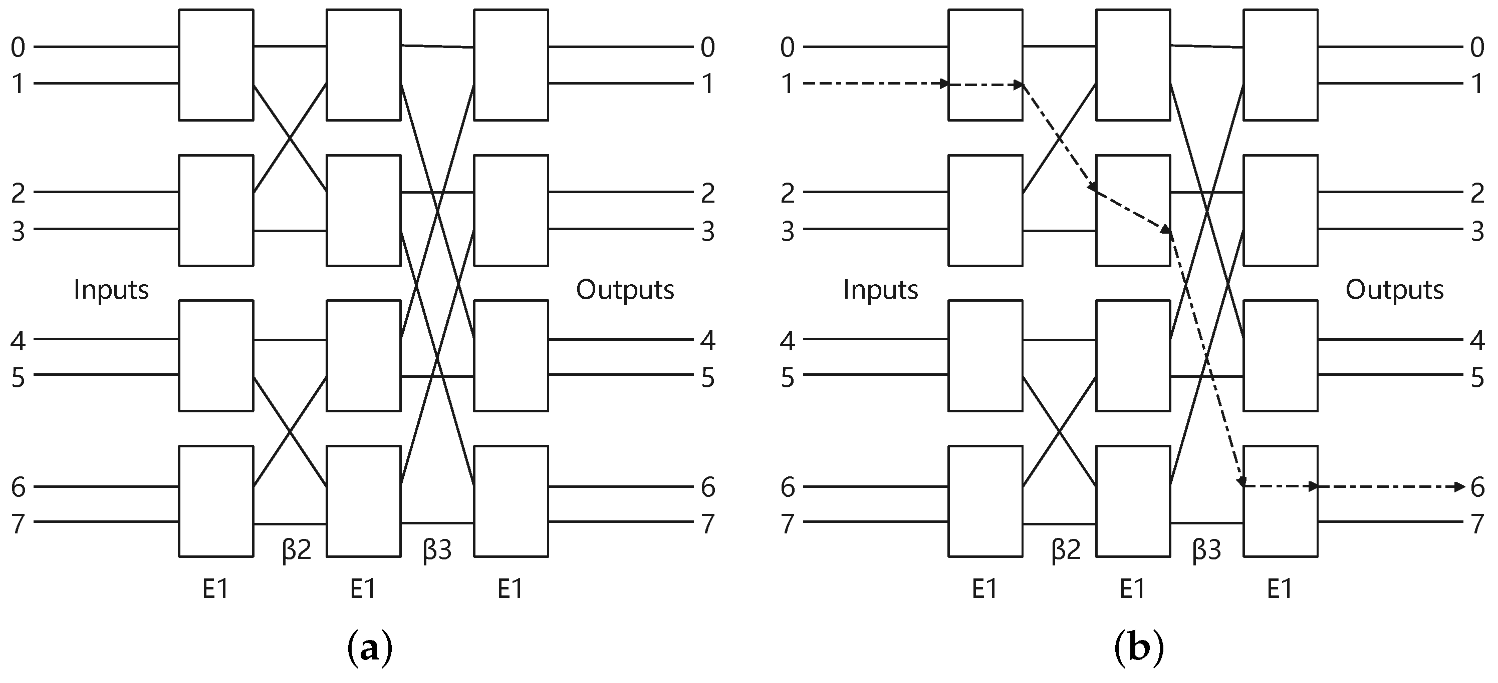
The shuffle-exchange network, like the Banyan network, Omega network, and indirect binary n-cube network, is a network that uses full shuffling functions and switching functions to realize interconnection between nodes. A topology diagram of the Banyan network with is shown in Figure 1a.
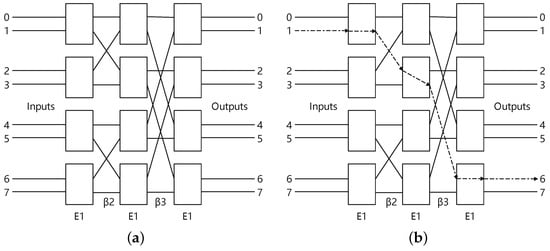
Figure 1.
The Banyan network. (a) The Banyan network. (b) The diffusion example in Banyan network.
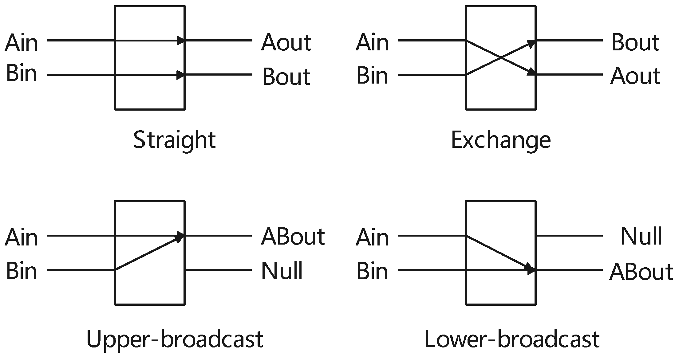
2.1.1. Exchange Unit
The exchange unit has two inputs and two outputs, serving as the fundamental component in various shuffle-exchange networks. Different multilevel interconnection networks employ distinct types of exchange units, topologies, and control methods. In general, there are four distinct switching states or connection modes, as illustrated in Figure 2: straight, exchange, upper-broadcast, and lower-broadcast. In our algorithm, we utilize straight and exchange switching units.

Figure 2.
The exchange unit.
2.1.2. Banyan Network
The Banyan network is a type of interconnection network, and its composite routing function is shown in Equation (1):
where represents the exchange unit and represents the ith replacement stage. For each control switch, we configure the exchange units in the straight state when and the exchange state when . As an example depicted in Figure 1b, when the input is 1 and the control signal is 010, the output is 6.
2.2. DNA Encoding
To use biocomputers in the future, the information processing techniques based on DNA coding have been studied. First of all, the information being processed will be encoded to four distinct nucleic acids, namely, A (adenine), T (thymine), C (cytosine), and G (guanine). According to the base pairing principle, A pairs with T and C pairs with G. Coincidentally, 0 and 1 are complementary in the binary system; therefore, 00 and 01 are regarded as complementary with 11 and 10. For example, when using encoding rules , , , and , can be encoded as and can be decoded as .
3. Proposed Chaotic System
The mathematical representation of the sin map is given by Equation (2):
where is the control parameter. As shown in Figure 3b, the sin map has some nonchaotic ranges when . Among the characteristics of chaotic systems, the positive Lyap exponent and orbital global bounding are widely used as evidence for judging chaos. According to the theory of the Chen-Lai algorithm [32], a high-gain feedback controller is constructed to obtain the positive Lyap exponent of the dynamic system. Furthermore, a modular operation to make the system globally bounded is designed. Drawing inspiration from the sin map and Chen-Lai algorithm, we construct a 1-DSCM, which is depicted in Equation (3).
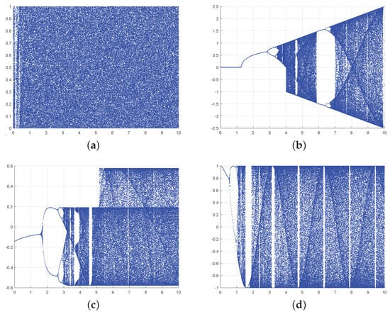
Figure 3.
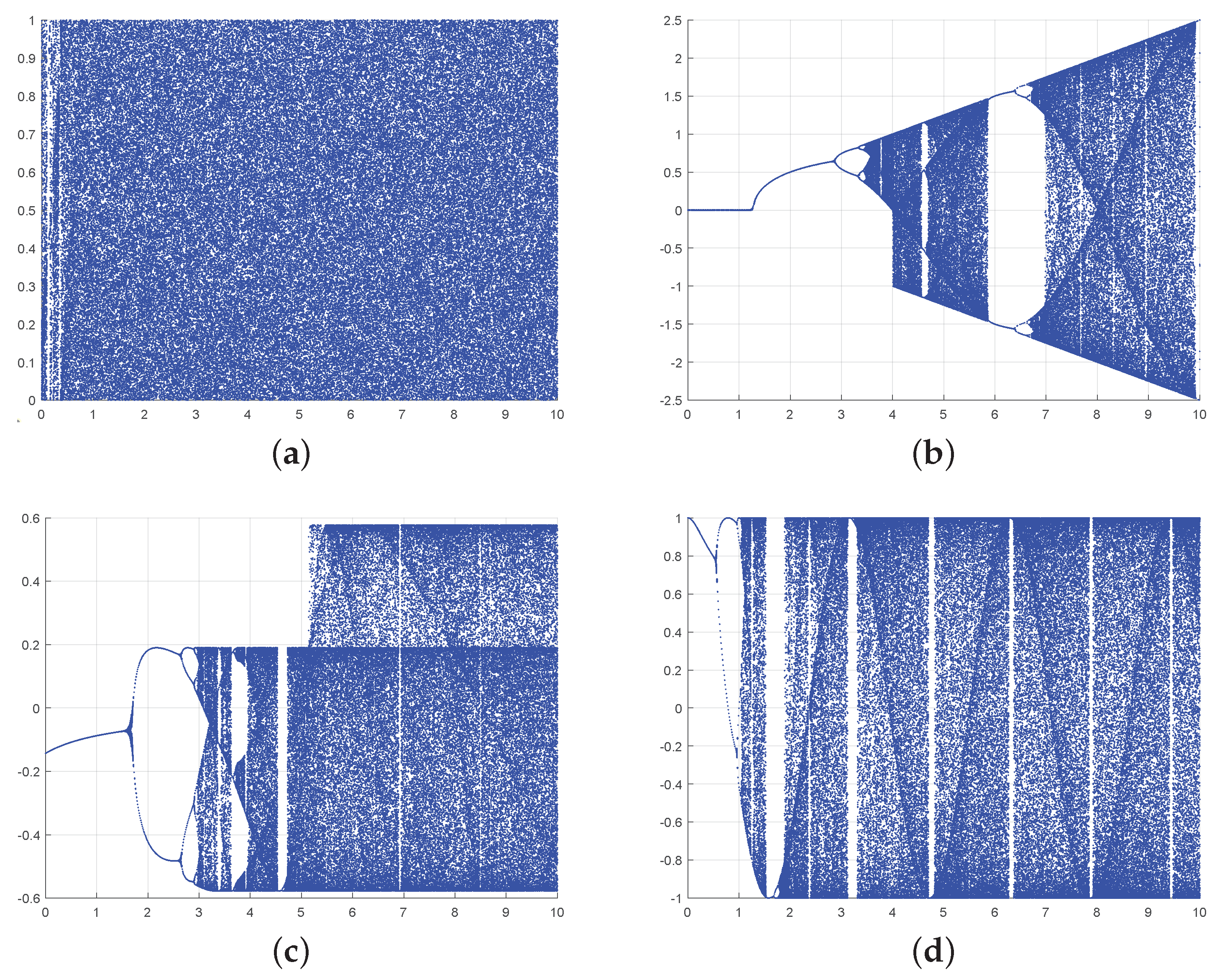
The bifurcation diagram of 1-DSCM, 1-DFCS, and 1-DCP. (a) The bifurcation diagram of 1-DSCM with . (b) The bifurcation diagram of sin map with . (c) The bifurcation diagram of 1-DFCS with . (d) The bifurcation diagram of 1-DCP with .
Here, r is the control parameter of the 1-DSCM. To evaluate the performance of the 1-DSCM, various tests, including Lyapunov exponent test, bifurcation analysis, sample entropy, 0-1 test, and NIST test, are performed in the following subsections.
3.1. Lyapunov Exponent Test
The Lyapunov exponent (LE), which signifies the rate of separation between neighboring trajectories, serves as a pivotal criterion in assessing the chaotic nature of a dynamic system . The definition of the Lyapunov exponent is presented in Equation (4).
where n represents the dimension of the generated time series . A positive Lyapunov exponent (LE) means the high sensitivity to the initial value. Moreover, the larger the LE value is, the better the chaotic behavior of the system is. The LE values of the sin map 1-DFCS [3], 1-DCP [4], and 1-DSCM are provided in Figure 4. As illustrated in Figure 4, compared to other recently proposed chaotic systems, 1-DSCM exhibits higher Lyapunov exponent (LE) value across a broader parameter range.
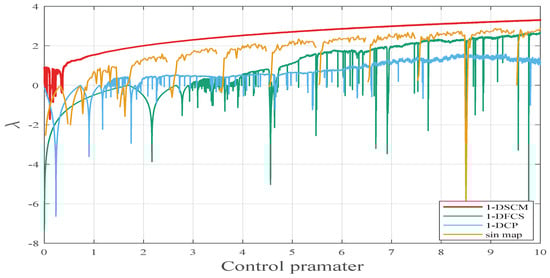
Figure 4.
The Lyapunov exponent of 1-DSCM, 1-DFCS, 1-DCP, and sin map with .
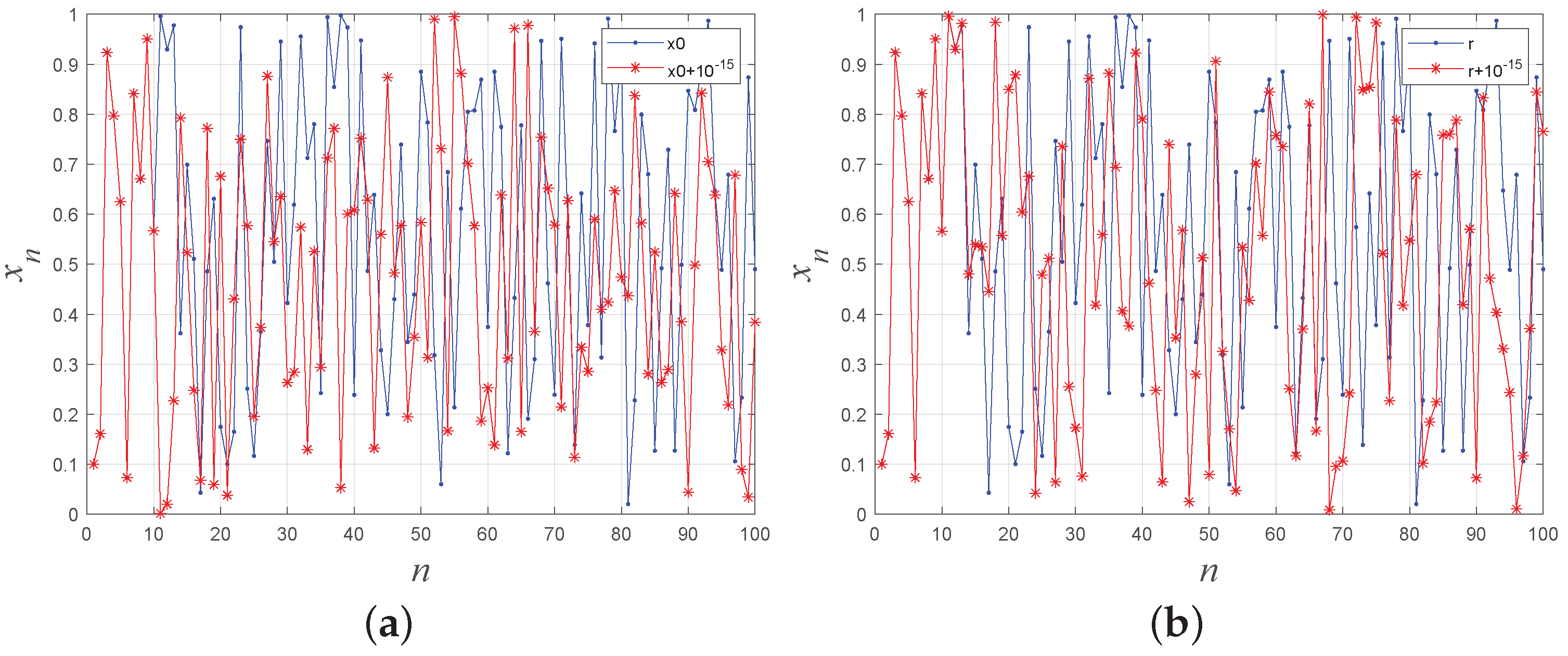
For a visual assessment of the proposed system’s sensitivity to initial values and control parameters, the generated chaotic sequences with a slight variation in initial values or control parameters are plotted in Figure 5, providing evidence of 1-DSCM’s high sensitivity to initial values and control parameters.
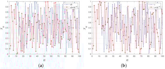
Figure 5.
(a) The sensitivity of the initial value. (b) The sensitivity of the control parameter.
3.2. Bifurcation Analysis
The dynamics of a system can be effectively depicted through the diagram of bifurcation. In Figure 3, we present the bifurcation diagrams for the 1-DSCM, 1-DFCS, and 1-DCP. In comparison to other chaotic systems, 1-DSCM displays a more extensive chaotic region and without the emergence of periodic phases.
3.3. Sample Entropy
The time series’ self-similarity of chaotic systems can be quantified through sample entropy (SE) [33]. A larger SE value indicates higher complexity in the dynamic behavior and lower regularity in the time series. The SE value for the time series X can be modeled by Equations (5)–(7):
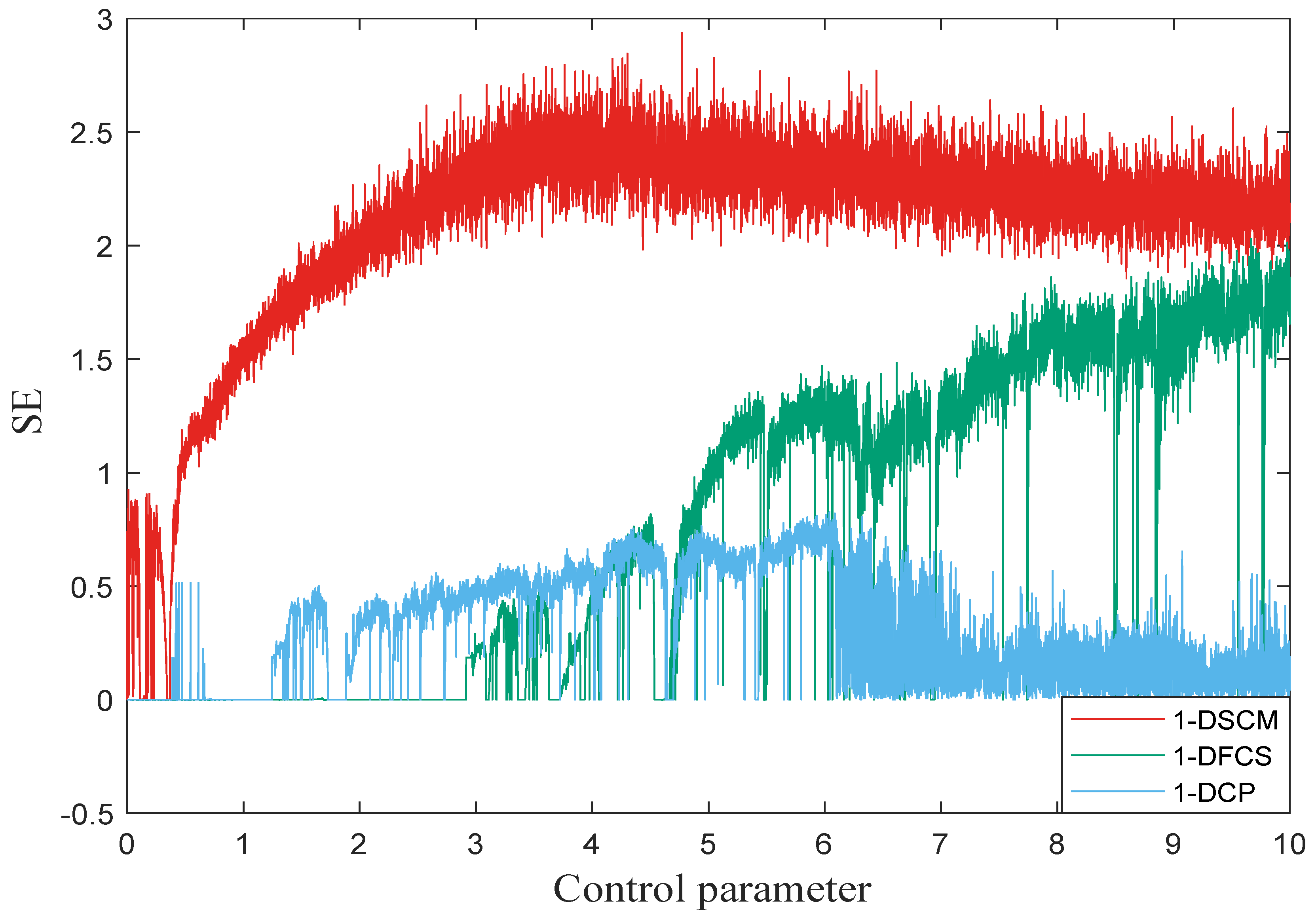
where is the Chebyshev distance between to , r is the specified distance, represents the template vector, and and are the counts of vectors that satisfy the conditions and , respectively. We set in our simulation, and the comparative analysis results of 1-DSCM with other chaotic systems are provided in Figure 6. This analysis proves that 1-DSCM exhibits superior performance in SE analysis to other chaotic systems.

Figure 6.
The sample entropy of 1-DSCM, 1-DFCS, and 1-DCP with .
3.4. 0-1 Test
In this subsection, we utilize 0-1 test to judge the chaotic status of 1-DSCM, 1-DFCS, and 1-DCP. The K value can be calculated using Equations (8)–(11):
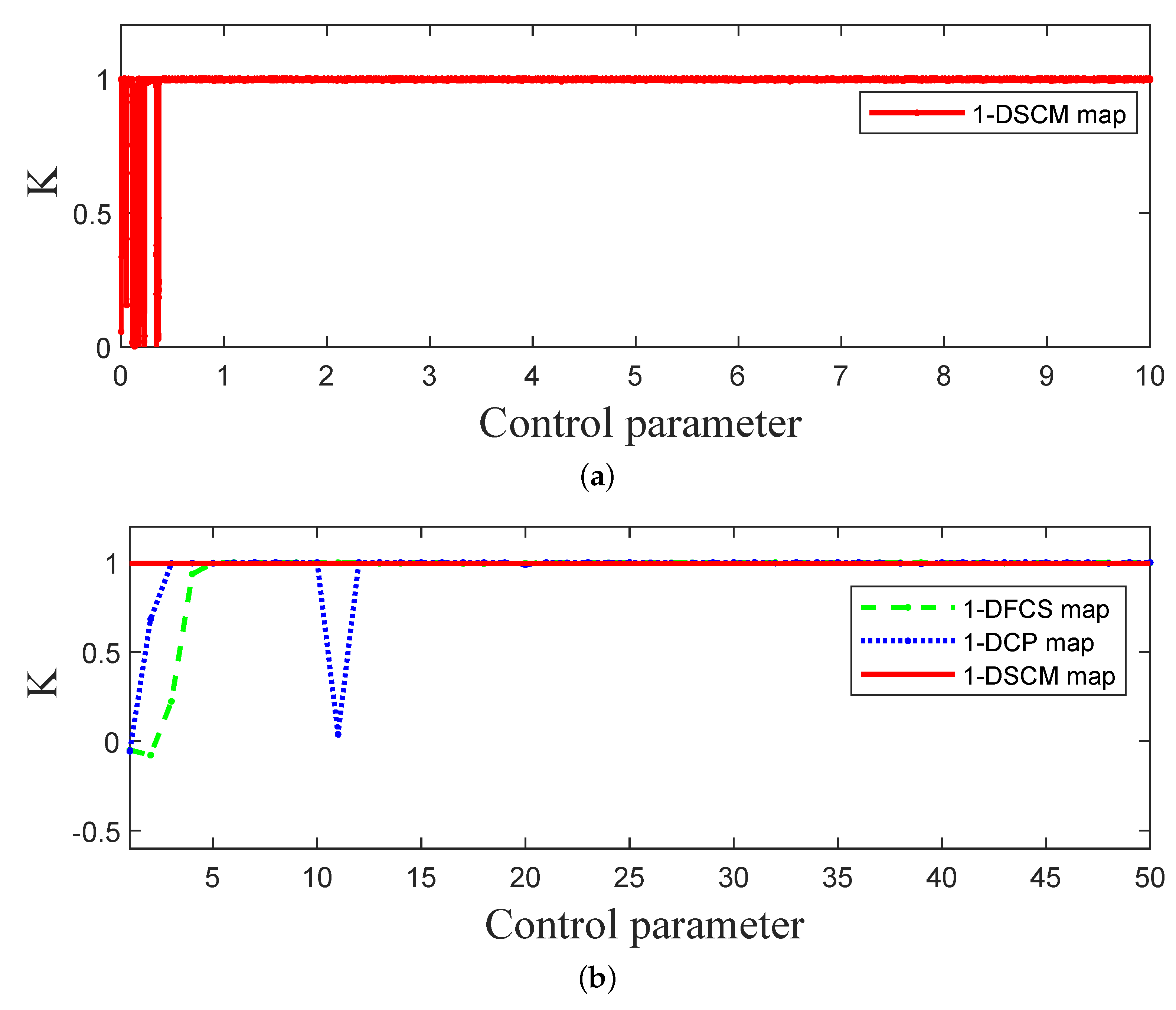
where X represents the sequence of size N generated by the 1-DSCM. Here, we set , and the value of K close to 1 indicates that the dynamic system is in a chaotic state. Figure 7 depicts the outcomes of the 0-1 test for 1-DSCM, 1-DFCS, and 1-DCP. The results demonstrate that the K scores of 1-DSCM are close to 1.
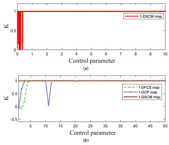
Figure 7.
The 0-1 test of 1-DSCM, 1-DFCS, and 1-DCP. (a) The 0-1 test of 1-DSCM with . (b) The 0-1 test of 1-DSCM, 1-DCP, and 1-DFCS with .
3.5. NIST SP 800-22 Test
We utilize the National Institute of Standards and Technology (NIST) SP 800-22 test suite to further validate the randomness of the sequences generated by the 1-DSCM. Firstly, a time series with 12,500,000 values, which is denoted as , is generated by the 1-DSCM. Then, the values of are mapped into the interval 0 to 255 using Equation (12):
Finally, the integer part of each value in is transformed to 8 bits. The test results are presented in Table 1, where all p-values fall within the range . This affirms that the sequence produced by the 1-DSCM processes high randomness and it is suitable for image encryption.

Table 1.
NIST test results of 1-DSCM.
4. Banyan Network-DNA Mapping
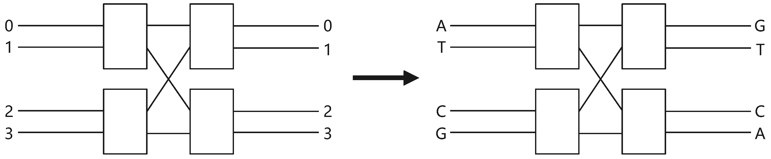
In this section, based on the characteristic of DNA encoding, we constructed a novel DNA mapping using an Banyan network. The topological graph of the Banyan network is demonstrated on the left of Figure 8. Here, we set input ports 0–3 that correspond to ATCG, respectively, and output ports 0–3 that correspond to GTCA, respectively, which is illustrated on the right of Figure 8. The Banyan network-DNA mapping rule is given in Table 2.
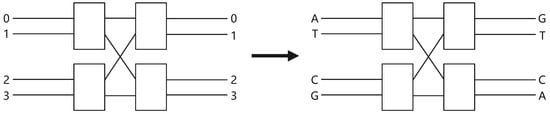
Figure 8.
The Banyan network-DNA mapping.
Table 2.
Banyan network-DNA mapping rules.
5. Encryption Framework
In this paper, we present a novel image encryption framework using the technology of the Banyan network to obtain a better diffusion effect. The flow chart of our algorithm is shown in Figure 9.

Figure 9.
The flow chart of our algorithm.
Step 1: A natural image P() is first input into the SHA-256 hash function to yield a 256-bit hash value h.
Step 2: Subsequently, the h is further divided into eight discrete segments to obtain using Equation (13).
where is a temporary variable.
Step 3: Four sequences, , shown in Equation (14) with the size of , respectively, are generated by 1-DSCM using the key , and the first iteration values are discarded.
According to Equation (15), these sequences are processed to obtain to be used in the continued stages.
Step 5: We insert the parameter into . Firstly, we generate a null vector and add it to the last row of the image . Secondly, the value of the -th element in is changed to . The position can be calculated by Equation (17). It is worth noting that the size of now becomes .
Step 6: We perform a row permutation operation using X and a column permutation operation using Y. The details of the scrambling procedure are displayed in Algorithm 1.
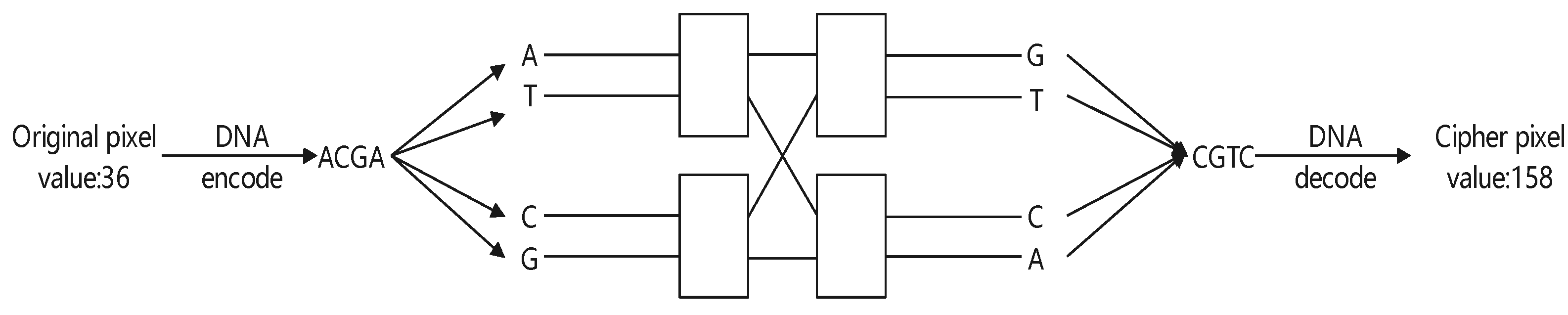
Step 7: We perform the Banyan network diffusion operation. Each pixel of is encoded into four nucleic acids which are input into the Banyan network-DNA mapping shown in Figure 8. Using the W as the control signal, the output of the Banyan network-DNA mapping is obtained and then decoded to obtain the corresponding cipher pixel. The final encrypted image is denoted as . For example, as per the example detailed in Section 2.2, 36 can be encoded as . When the control signal of the Banyan network is 10, the output is , which can be decoded into a cipher pixel value of 158. A visualization of the example is shown in Figure 10.
| Algorithm 1 Encryption algorithm. |
Input: The original image P, parameter and four chaotic sequences X, Y, Z, W. Output: Encrypted image .
|
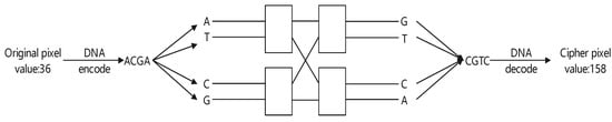
Figure 10.
Example of Banyan network diffusion operation.
Decryption is the converse methodology to encryption, elucidated in Algorithm 2.
| Algorithm 2 Decryption algorithm. |
Input: The encrypted image and four sequences X, Y, Z and W. Output: The original image P.
|
6. Simulation Results
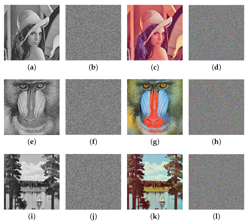
In this section, the evaluation of the proposed cryptosystem through distinct experimental analyses is given. Experiments were performed on a personal computer with Matlab R2021a software in Windows 11 operating system. The natural and encrypted images are visually presented in Figure 11.
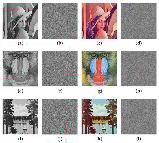
Figure 11.
The original and cipher images. (a) Lena gray image. (b) Encrypted image of gray Lena. (c) Lena color image. (d) Encrypted image of color Lena. (e) Baboon gray image. (f) Encrypted image of gray baboon. (g) Baboon color image. (h) Encrypted image of color baboon. (i) Sailboat gray image. (j) Encrypted image of gray sailboat. (k) Sailboat color image. (l) Encrypted image of color sailboat.
6.1. Plaintext Sensitivity
A cryptosystem with high security should be sensitive to a small change in plaintext to resist differential power attacks (DPAs). The number of pixels changing rate (NPCR) and the unified averaged changed intensity (UACI) can be used to assess the ability of encryption algorithms against DPA [34]. NPCR and UACI are calculated as follows:
where and are two cipher images corresponding to two natural images differing by a single pixel and . The vertical and horizontal dimensions of the images are denoted as M and N, respectively. As shown in Table 3, our system exhibits strong robustness against differential attacks.
Table 3.
NPCR and UACI analysis for plaintext sensitivity of different algorithms.
6.2. Exhaustive Attack Analysis
6.2.1. Security Key Space
According to [35], the key space of an encryption algorithm should not be less than to protect against brute-force attacks. Our encryption framework incorporates an ensemble of secret keys, denoted as , , and . It is assumed that the computational precision of the system is and the key space can be described as . This provides evidence for the inherent strength of our encryption algorithm to withstand brute-force attacks.
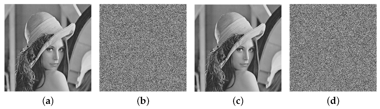
6.2.2. Secret Key Sensitivity
A strong cryptosystem should have high sensitivity to the key. From Figure 12, a slight change in the key will make the decrypted image distort completely. Furthermore, the NPCR and UACI test results are displayed in Table 4. This demonstrates that the proposed algorithm is highly dependent on the key.
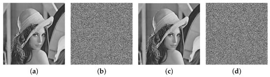
Figure 12.
The original, encrypted, and decrypted images. (a) The plain image. (b) The encrypted image. (c) The decrypted image with correct key. (d) The decrypted image with .
Table 4.
Key sensitivity analysis.
6.3. Statistical Attack Analysis
6.3.1. Correlation Coefficient Test
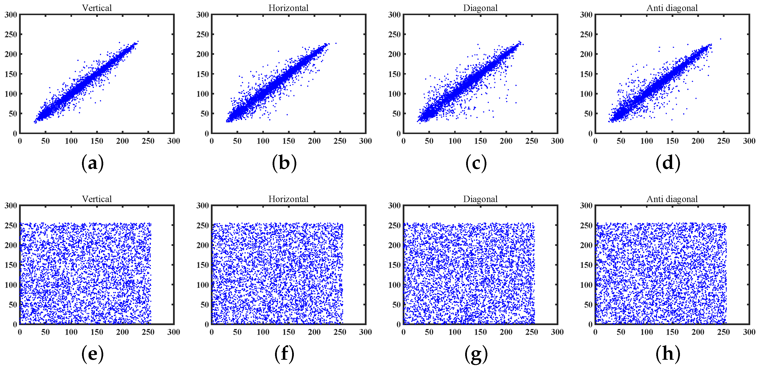
In natural images, neighboring pixels consistently display a notable correlation. To counteract statistical attacks, the correlation among neighboring pixels is expected to be disrupted after encryption. The correlation coefficient of a gray image is described by Equation (19):
where two variables, x and y, denote adjacent pixel values derived from four orientations.
We chose 5000 pixel pairs from both the original and encrypted Lena images in four directions to calculate the correlation coefficient, and the results are outlined in Table 5. In addition, the corresponding correlation distributions of these images are graphically presented in Figure 13. It can be observed that our encryption algorithm possesses excellent performance in eliminating the inherent correlations of neighbor pixels in natural images.
Table 5.
Correlation analysis of original images and encrypted images.
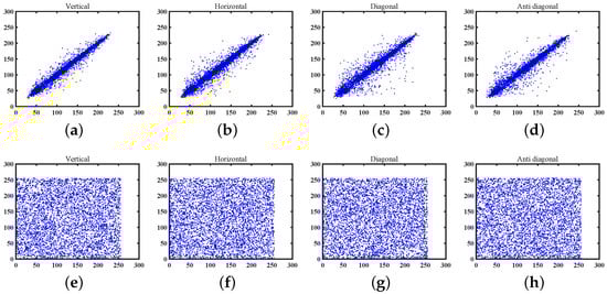
Figure 13.
The correlation coefficient of Lena. (a) Vertical correlation. (b) Horizontal correlation. (c) Diagonal correlation. (d) Antidiagonal correlation. (e) Vertical correlation of encrypted image. (f) Horizontal correlation of encrypted image. (g) Diagonal correlation of encrypted image. (h) Antidiagonal correlation of encrypted image.
6.3.2. Histogram Analysis
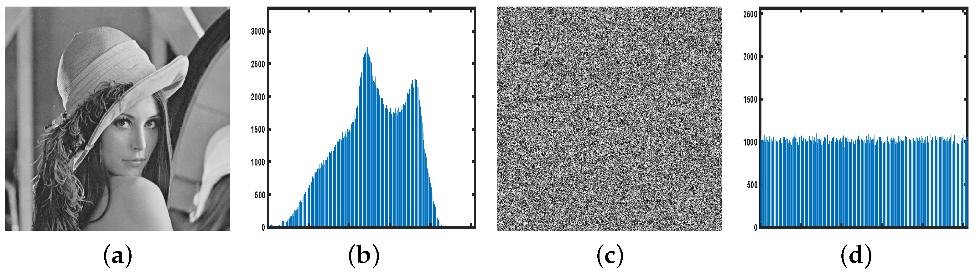
To resist statistical attacks, histogram of the encrypted image should be flat. Figure 14 displays the histograms of both the original and encrypted images, illustrating that all pixel values appear almost equally frequently. Therefore, it is impossible for attackers to acquire relevant statistics that could enable the inference of original image information.
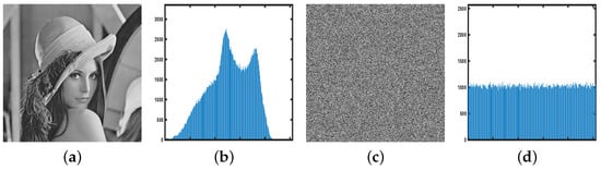
Figure 14.
The histogram analysis. (a) The natural image. (b) Histogram of the natural image. (c) The cipher image. (d) Histogram of the cipher image.
Furthermore, the flatness of the histogram can be tested through the test, which can be calculated by Equation (20):
where i denotes the gray level and represents the frequency of the gray level i within the image. When the significance level and the outcome of the test falls below , the test passes. Table 6 implies that all cipher images achieve a satisfactory level of histogram flatness.
Table 6.
test result of gray images .
6.3.3. Information Entropy Analysis
Information entropy is often used to quantify the uncertainty of information. The theoretical value of the 256-level information source is 8. The formula of information entropy is given by Equation (21):
where represents the value of each level. It can be observed from Table 7 that the of the cipher image is close to 8, proving that the images encrypted by our algorithm exhibit a high level of randomness.
Table 7.
The information entropy of gray images.
6.4. Encrypted Time Analysis
When a cryptosystem is utilized on a resource-limited platform or scenario that requires real-time encryption, low time complexity is crucial. Assuming that the size of the original image is , the time complexity of the first diffusion operation and row–column permutation stage are both . The time complexity of the Banyan network diffusion stage is . Therefore, the time complexity of the whole algorithm is . Furthermore, encrypted time analysis is given in this subsection. The overall encryption time comprises several components: iteration of the chaotic sequence, the first diffusion, row–column permutation, and Banyan network diffusion. Table 8 displays the results of the comparable encryption time analysis with other similar algorithms [10,12,23,27,28], indicating that our cryptosystem is highly efficient in encryption and has the potential for real-time encryption.
Table 8.
Time required for encryption (in seconds) of each gray image.
6.5. Chosen-Plaintext Attack Analysis
Attackers often employ the chosen/known-plaintext attacks to deduce the secret keys or reveal the underlying correlation between plaintexts and ciphertexts. For instance, attackers may deliberately select or generate a specific plaintext, such as an all-black or an all-white image, to obtain the corresponding ciphertext. As illustrated in Figure 15, the encrypted image exhibits noise-like characteristics, preventing attackers from deriving any meaningful information from it.
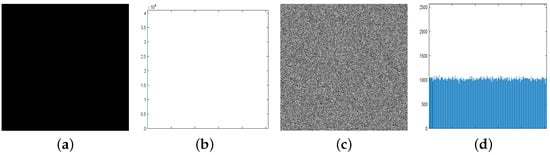
Figure 15.
Chosen-plaintext attack analysis. (a) All-black image. (b) Histogram of all-black image. (c) The cipher image. (d) Histogram of cipher image.
6.6. PSNR Analysis
The peak signal-to-noise ratio is a metric used to assess image quality and can be used to judge the dissimilarities between the ciphertext image and the plaintext image. Its formulation is delineated in Equation (22).
where H and W are the dimensions of images and . A lower PSNR value between the original image and the encrypted image means a higher level of randomness of the cipher image. As shown in Table 9, our algorithm has a high quality of encryption.
Table 9.
PSNR value of cipher image.
6.7. Noise Attack and Cropping Attack Analysis
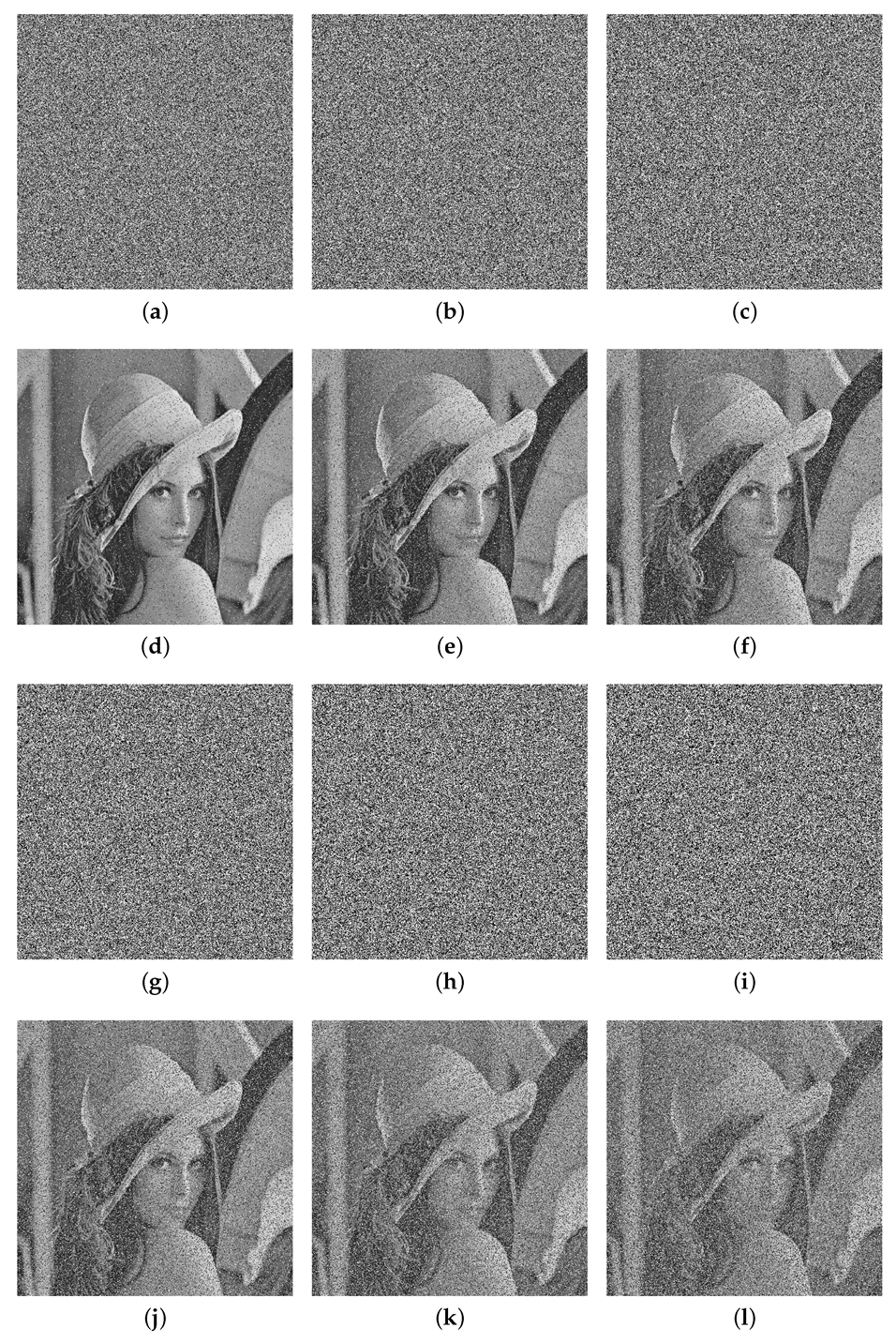
When transmitting encrypted data over public channels, they may suffer from noise effect or data loss. From Figure 16 and Figure 17 and Table 10, our algorithm has a strong robustness against the noise attack and the cropping attack, which means that the main information of the original image can be recovered when the cipher image suffers from the noise effect or data loss.
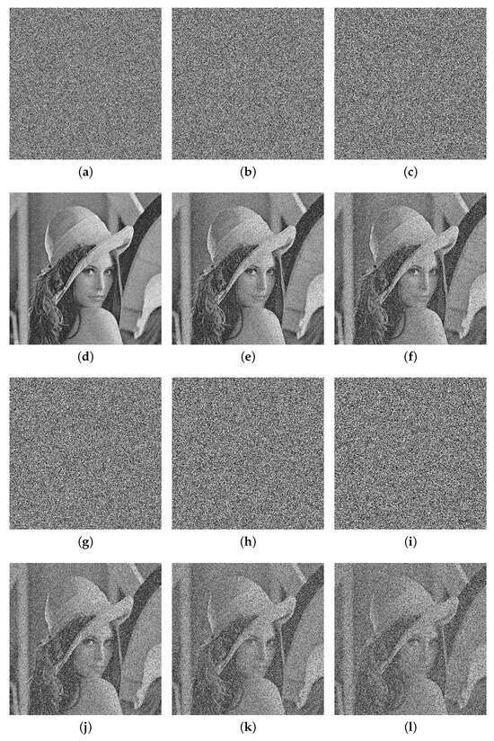
Figure 16.
The Salt and pepper noise attack of Lena. (a) 0.1 Salt and pepper. (b) 0.2 Salt and pepper. (c) 0.3 Salt and pepper. (d) Decryption image of (a). (e) Decryption image of (b). (f) Decryption image of (c). (g) 0.4 Salt and pepper. (h) 0.5 Salt and pepper. (i) 0.6 Salt and pepper. (j) Decryption image of (g). (k) Decryption image of (h). (l) Decryption image of (i).
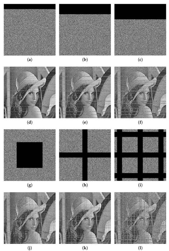
Figure 17.
The cropping attack of Lena. (a) Cropping attack (). (b) Cropping attack (). (c) Cropping attack (). (d) Decryption image of (a). (e) Decryption image of (b). (f) Decryption image of (c). (g) Cropping attack (). (h) Cropping attack (≈). (i) Cropping attack (≈). (j) Decryption image of (g). (k) Decryption image of (h). (l) Decryption image of (i).
Table 10.
PSNR value of noise attack.
7. Conclusions
This paper introduces a novel 1-D chaotic system 1-DSCM, and several tests, such as 0-1 test and NIST test, were performed to prove its better performance in chaotic behavior and parameters’ structure than the sin map. In addition, a new image encryption algorithm was conducted using 1-DSCM, SHA-256 hash function, and Banyan network. Taking advantage of the 1-DSCM, which can generate pseudorandom sequences quickly, and the Banyan network, which can offer parallel operation and nonlinearity, the proposed encryption algorithm processes high security and efficiency. Complete experiments show that our system has excellent performance in security and encryption speed, and it is more suitable for the scenarios requiring real-time encryption or with limited resources. In the future, we will implement the proposed encryption algorithm on an FPGA to verify the effectiveness of the network’s parallel operation in image encryption and the feasibility of the encryption system in video encryption.
Author Contributions
Conceptualization, H.Z.; data management, S.C.; formal analysis, X.X.; access to funds, S.C.; survey, X.X.; methodology, Q.H. and H.Z.; project management, H.Z.; software, Q.H.; supervision, H.Z.; verification, Q.H.; visualization, Q.H.; writing—manuscript, Q.H.; writing—review and editing, L.H. and H.Z. All authors have read and agreed to the published version of the manuscript.
Funding
This work was funded by the Key Area R & D Program of Guangdong Province under Grant 2022B0701180001, the National Natural Science Foundation of China (61801127), the Science Technology Planning Project of Guangdong Province, China (No. 2019B010140002, No. 2020B111110002), and the Guangdong–Hong Kong–Macao Joint Innovation Field Project (No. 2021A0505080006).
Data Availability Statement
Not applicable.
Acknowledgments
The authors are thankful to the reviewers for their comments and suggestions that improved the quality of the manuscript.
Conflicts of Interest
The authors declare no conflict of interest. The founding sponsors had no role in the design of the study; in the collection, analyses, or interpretation of data; in the writing of the manuscript, and in the decision to publish the results.
References
- Wu, Y.; Zeng, J.; Dong, W.; Li, X.; Qin, D.; Ding, Q. A Novel Color Image Encryption Scheme Based on Hyperchaos and Hopfield Chaotic Neural Network. Entropy 2022, 24, 1474. [Google Scholar] [CrossRef]
- Wang, Y.; Yang, F. A fractional-order CNN hyperchaotic system for image encryption algorithm. Phys. Scr. 2020, 96, 035209. [Google Scholar] [CrossRef]
- Midoun, M.A.; Wang, X.; Talhaoui, M.Z. A sensitive dynamic mutual encryption system based on a new 1D chaotic map. Opt. Lasers Eng. 2021, 139, 106485. [Google Scholar] [CrossRef]
- Talhaoui, M.Z.; Wang, X.; Midoun, M.A. A new one-dimensional cosine polynomial chaotic map and its use in image encryption. Vis. Comput. 2021, 37, 541–551. [Google Scholar] [CrossRef]
- Chang, H.; Wang, E.; Liu, J. A Novel Chaotic Image Encryption Algorithm Based on Propositional Logic Coding. Int. J. Bifurc. Chaos 2023, 33, 2350089. [Google Scholar] [CrossRef]
- Wan, Y.; Wang, S.; Du, B. A bit plane image encryption algorithm based on compound chaos. Multimed. Tools Appl. 2023, 82, 22103–22121. [Google Scholar] [CrossRef]
- Wang, J.; Li, J.; Di, X.; Zhou, J.; Man, Z. Image Encryption Algorithm Based on Bit-Level Permutation and Dynamic Overlap Diffusion. Multidisciplinary 2020, 8, 160004–160024. [Google Scholar] [CrossRef]
- Li, Z.; Peng, C.; Tan, W.; Li, L. A Novel Chaos-Based Color Image Encryption Scheme Using Bit-Level Permutation. Symmetry 2020, 12, 1497. [Google Scholar] [CrossRef]
- Zhao, Y.; Liu, L. A Bit Shift Image Encryption Algorithm Based on Double Chaotic Systems. Entropy 2021, 23, 1127. [Google Scholar] [CrossRef]
- Wang, X.; Li, Y.; Jin, J. A new one-dimensional chaotic system with applications in image encryption. Chaos Solitons Fractals 2020, 139, 110102. [Google Scholar] [CrossRef]
- Wang, X.; Gao, S. A chaotic image encryption algorithm based on a counting system and the semi-tensor product. Multimed. Tools Appl. 2021, 80, 10301–10322. [Google Scholar] [CrossRef]
- Huang, S.; Jiang, D.; Wang, Q.; Guo, M.; Huang, L.; Li, W.; Cai, S. High-quality visually secure image cryptosystem using improved Chebyshev map and 2D compressive sensing model. Chaos Solitons Fractals 2022, 163, 112584. [Google Scholar] [CrossRef]
- Zhang, T.; Wang, S. Image encryption scheme based on a controlled zigzag transform and bit-level encryption under the quantum walk. Front. Phys. 2023, 10, 1097754. [Google Scholar] [CrossRef]
- Gao, X.; Mou, J.; Xiong, L.; Sha, Y.; Yan, H.; Cao, Y. A fast and efficient multiple images encryption based on single-channel encryption and chaotic system. Nonlinear Dyn. 2020, 108, 613–636. [Google Scholar] [CrossRef]
- Hoang, T.M. A novel design of multiple image encryption using perturbed chaotic map. Multimed. Tools Appl. 2020, 81, 26535–26589. [Google Scholar] [CrossRef]
- Jiang, X.; Jiang, G.; Wang, Q.; Shu, D. Image encryption algorithm based on 2D-CLICM chaotic system. IET Image Process. 2023, 17, 2127–2141. [Google Scholar] [CrossRef]
- Lin, H.; Wang, C.; Du, S.; Yao, W.; Sun, Y. A family of memristive multibutterfly chaotic systems with multidirectional initial-based offset boosting. Chaos Solitons Fractals 2023, 172, 113518. [Google Scholar] [CrossRef]
- Yu, F.; Kong, X.; Mokbel, A.A.M.; Yao, W.; Cai, S. Complex Dynamics, Hardware Implementation and Image Encryption Application of Multiscroll Memeristive Hopfield Neural Network With a Novel Local Active Memeristor. IEEE Trans. Circuits Syst. II Express Briefs 2023, 70, 326–330. [Google Scholar] [CrossRef]
- Singh, K.N.; Singh, O.P.; Singh, A.K. ECiS: Encryption prior to compression for digital image security with reduced memory. Comput. Commun. 2022, 193, 410–441. [Google Scholar] [CrossRef]
- Babaei, A.; Motameni, H.; Enayatifar, R. A new permutation-diffusion-based image encryption technique using cellular automata and DNA sequence. Optik 2020, 203, 164000. [Google Scholar] [CrossRef]
- Yildirim, M. Optical color image encryption scheme with a novel DNA encoding algorithm based on a chaotic circuit. Chaos Solitons Fractals 2022, 155, 111631. [Google Scholar] [CrossRef]
- Feng, W.; He, Y.; Li, H.; Li, C. Cryptanalysis and Improvement of the Image Encryption Scheme Based on Feistel Network and Dynamic DNA Encoding. IEEE Access 2019, 7, 12584–12597. [Google Scholar] [CrossRef]
- Kang, Y.; Huang, L.; He, Y.; Xiong, X.; Cai, S.; Zhang, H. On a Symmetric Image Encryption Algorithm Based on the Peculiarity of Plaintext DNA Coding. Symmetry 2020, 12, 1393. [Google Scholar] [CrossRef]
- Azam, N.A.; Ullah, I.; Hayat, U. A fast and secure public-key image encryption scheme based on Mordell elliptic curves. Opt. Lasers Eng. 2021, 137, 106371. [Google Scholar] [CrossRef]
- Zheng, J.; Bao, T. An Image Encryption Algorithm Using Cascade Chaotic Map and S-Box. Entropy 2022, 24, 1827. [Google Scholar] [CrossRef] [PubMed]
- Nematzadeh, H.; Enayatifar, R.; Yadollahi, M.; Lee, M.; Jeong, G. Binary search tree image encryption with DNA. Opt. Z. Fur Licht- Und Elektron. J. Light Electronoptic 2020, 202, 163505. [Google Scholar] [CrossRef]
- Huang, L.; Li, W.; Xiong, X.; Yu, R.; Wang, Q.; Cai, S. Designing a double-way spread permutation framework utilizing chaos and S-box for symmetric image encryption. Opt. Commun. 2022, 517, 128365. [Google Scholar] [CrossRef]
- Arslan Shafque, F.A. Image Encryption Using Dynamic S-Box Substitution in the Wavelet Domain. Wirel. Pers. Commun. 2020, 115, 2243–2268. [Google Scholar] [CrossRef]
- Xie, Z.; Sun, J.; Tang, Y.; Tang, X.; Simpson, O.; Sun, Y. A K-SVD Based Compressive Sensing Method for Visual Chaotic Image Encryption. Mathematics 2023, 11, 1658. [Google Scholar] [CrossRef]
- Skanda, C.; Srivatsa, B.; Premananda, B. Design of Compact and Energy Efficient Banyan Network for Nano Communication. In Proceedings of the 2021 IEEE International Conference on Distributed Computing, VLSI, Electrical Circuits and Robotics (DISCOVER), Nitte, India, 19–20 November 2021; pp. 135–140. [Google Scholar] [CrossRef]
- Ali, M.M.; Madhupriya, G.; Indhumathi, R.; Krishnamoorthy, P. Performance enhancement of 8×8 dilated banyan network using crosstalk suppressed GMZI crossbar photonic switches. Photonic Netw. Commun. 2021, 42, 123–133. [Google Scholar] [CrossRef]
- Chen, G.; Lai, D. Feedback control of Lyapunov exponents for discrete-time dynamical systems. Int. J. Bifurc. Chaos 1996, 6, 1341–1349. [Google Scholar] [CrossRef]
- Richman, J.S.; Moorman, J.R. Physiological time-series analysis using approximate entropy and sample entropy. Am. J. Physiol.-Heart Circ. Physiol. 2000, 278, H2039–H2049. [Google Scholar] [CrossRef] [PubMed]
- Wu, Y.; Noonan, J.P.; Agaian, S. NPCR and UACI randomness tests for image encryption. Cyber J. Multidiscip. J. Sci. Technol. J. Sel. Areas Telecommun. (JSAT) 2011, 1, 31–38. [Google Scholar]
- Alvarez, G.; Li, S. Some basic cryptographic requirements for chaos-based cryptosystems. Int. J. Bifurc. Chaos 2006, 16, 2129–2151. [Google Scholar] [CrossRef]


Disclaimer/Publisher’s Note: The statements, opinions and data contained in all publications are solely those of the individual author(s) and contributor(s) and not of MDPI and/or the editor(s). MDPI and/or the editor(s) disclaim responsibility for any injury to people or property resulting from any ideas, methods, instructions or products referred to in the content. |
© 2023 by the authors. Licensee MDPI, Basel, Switzerland. This article is an open access article distributed under the terms and conditions of the Creative Commons Attribution (CC BY) license (https://creativecommons.org/licenses/by/4.0/).