Risk Premium of Bitcoin and Ethereum during the COVID-19 and Non-COVID-19 Periods: A High-Frequency Approach

Abstract

This paper reports our findings on the return dynamics of Bitcoin and Ethereum using high-frequency data (minute-by-minute observations) from 2015 to 2022 for Bitcoin and from 2016 to 2022 for Ethereum. The main objective of modeling these two series was to obtain a dynamic estimation of risk premium with the intention of characterizing its behavior. To this end, we estimated the Generalized Autoregressive Conditional Heteroskedasticity in Mean with Normal-Inverse Gaussian distribution (GARCH-M-NIG) model for the residuals. We also estimated the other parameters of the model and discussed their evolution over time, including the skewness and kurtosis of the Normal-Inverse Gaussian distribution. Similarly, we determined the parameters that define the evolution of the estimated variance, i.e., the parameters related to the fitted past variance, square error and long-term average value. We found that, despite the market uncertainty during the COVID-19 emergency period (2020 and 2021), the selected cryptocurrencies’ return volatility and kurtosis were even greater for several other subperiods within our sample’s time frame. Our model represents an analytical tool that estimates the risk premium that should be delivered by Bitcoin and Ethereum and is therefore of interest to risk managers, traders and investors.

1. Introduction

The sanitary emergency associated with the COVID-19 pandemic induced much turbulence in most economic sectors and, naturally, in the financial markets. Its effects during 2020 and 2021 were significantly greater than those of the financial crisis of 2008 [1,2,3]. From an economic point of view, the two most significant consequences were high global inflation rates during 2022 (resulting from a complex combination of supply constrains in the product and labor markets and economic agents’ expectations) and the aggressive anti-recessionary policies implemented by many countries. In February 2022, inflation levels in the United States were recorded to be at a historical maximum of 7.9% (their highest in 20 years). Business and consumption worldwide were impacted, and the global economy underwent negative growth. For example, the US GDP saw a reduction of 19.2% between the last quarter of 2019 and the second quarter of 2020, with the unemployment rate reaching 14.7% in April 2020, its highest level since 1948; this represented 23.1 million people without jobs. Between March 21st and July 18th 2020, 52.7 million citizens applied for unemployment insurance [4]. As an example of extraordinary anti-recessionary policies, the monetary measures taken by the United States government and its central bank represented an almost six trillion-dollar injection of money to the economy, and the reference interest rate dropped to almost zero.

Financial markets experienced their worse crash since the 2008–2009 turmoil. With huge transfers of money from the stock market to treasury bonds, the stock market’s upward trend that had lasted since 2009 finally ended. The turning point can be identified as March 2020, when the sanitary emergency and its associated constraints hit the market. However, significant recovery was observed during the second quarter of 2020, a period in which the Dow Jones Industrial Average, the S&P 500 and the NASDAQ increased by 18%, 20% and 31%, respectively [5].

The behavior of the cryptocurrency market was significantly different, which requires some explanation. Cryptocurrency trading is supported by Blockchain technology, a platform with the following distinctive characteristics:

(1)

There are no financial intermediaries, i.e., there is no middleman between buyers and sellers. It is a peer-to-peer technology, according to Harwick [6] and Dwyer [7].

(2)

It is decentralized and the government cannot control it, at least theoretically, as proposed by Dwyer [7] and Rose [8].

(3)

In terms of security, if the network has a problematic area, the non-affected areas can review the whole transaction flow with no problem. This is an important characteristic of Blockchain technology.

(4)

It is almost anonymous in its operation, Fang et al. [9].

(5)

It is open for operation 24 h, 7 days a week.

Since the introduction of Bitcoin and until December 2019, approximately 4950 cryptocurrencies were created (see Fang et al. [9]), and their market capitalization value was around 190 billion dollars in 2019. Bitcoin and Ethereum were the most important that year in terms of their market capitalization, representing 64% of the total in March [10].

Financial security time-varying risk premium estimation was introduced by Engle et al. [11], and led to a vast number of papers being published on this topic in the following decades. Authors who have analyzed the risk/return relationship using high-frequency data include Baron et al. [12], who use a sample of the leading Swedish equity index, the OMX S30; Almeida et al. [13], who study the S&P 500’s futures returns; and Ji [14], who works with the Shanghai 50. Breckenfelder [15] presents an interesting theoretical discussion on the tradeoff between risk and return using high-frequency data.

In this paper, we study the time dynamics of risk premium for Bitcoin and Ethereum during the COVID-19 and non-COVID-19 periods, using high-frequency data (minute-by-minute). A GARCH(1,1)-M-NIG model with 1440 daily observations was used because its parameters can be interpreted as an asset’s risk premium. To achieve improved adjustment, the residuals were modeled with a semi-heavy-tail distribution (Normal-Inverse Gaussian). This approach enables the observation of the model’s parameters throughout the observation period. Modeling the risk premium permits monitoring the behavior of Bitcoin and Ethereum to support investors in their decision making.

We hypothesized that the parameters of our model would show important variations during the COVID-19 and non-COVID-19 subperiods. We found that the former subperiod was not associated with the largest observed volatility during the analysis. The risk premium parameter varied considerably in subperiods that were different from the COVID-19 and non-COVID-19 subperiods. These variations were associated with time series bias and kurtosis, which, in addition to conveying valuable information for risk management (since we worked with intraday data), allowed us to better understand the behavior of Bitcoin and Ethereum. Our results indicate the existence of a relationship between price bubble episodes and exuberant behavior in the skewness and kurtosis of the returns distribution. The daily estimation of the model’s parameters supports finer calibration for risk managers and portfolio managers.

The interpretation of the GARCH model is straightforward and provides dynamic updates for supporting risk-management decisions. The variations in the parameters—which are random by nature—allow the dynamic behavior to be described with more precision to support decision making, especially when there are important variations. In contrast to other studies of high-frequency data (e.g., Pele et al. [16], Louzis [17], Degiannakis [18], Giot [19], Dionne [20] and Beltratti [21]), we present a model that explicitly shows the dynamic evolution of risk premium, not just the returns and volatility typically modeled by the GARCH Family models. While Gyamerah [22] uses the NIG distribution for residuals, they do not review the parameters of the distribution. To our knowledge, this is the first time that the behaviors of the skewness “$\rho$” and shape “$\zeta$” parameters are discussed using high-frequency data for Bitcoin and Ethereum. An additional contribution of this paper is that we developed GARCH-M-NIG modeling by day, i.e., we studied the evolution of the parameters with daily frequency, which was possible thanks to minute-by-minute data availability. The COVID-19 period did not show the largest variability during the period of study. Instead, the observed market bubbles of the previous year represented the period with the highest variance. This was reflected in the 2019 risk premium parameter.

This work provides a better understanding of the variability of Bitcoin and Ethereum by modeling their returns and volatility. The reported findings are expected to provide support for improving investments and risk management practices.

The remainder of this paper is structured as follows: Section 2 presents a literature review; Section 3 discusses the methodology used in our analysis; Section 4 contains a description of the data and presents the estimation results; and Section 5 concludes the paper.

2. Literature Review

Bitcoin was the first cryptocurrency introduced to the market and is currently the most important in its category; for these reasons, it has attracted a significant amount of of research attention. Studies of its returns’ volatility have used GARCH-type models, as in Bariviera et al. [23], Katsiampa [24] and Troster et al. [25] (note: Charles [26] re-estimated Katsiampa’s model using the same data and an extended observation set to find partially different results, and concluded that “GARCH-type models characterized by short memory, asymmetric effects, or long-run and short-run movements, seem not to be appropriate for modeling the Bitcoin returns”, contributing to a better understanding of this modeling technique).

Conrad [27] found that Bitcoin volatility has an inverse relationship with the volatility of the S&P500, and at the same time exhibits pro-cyclical behavior relative to the behavior of gold in periods of higher S&P500 volatility. In a related study, Al-Khazali et al. [28] discovered an asymmetric response between Bitcoin and gold volatility in the presence of positive or negative macroeconomic news.

Wen [29] demonstrated that Bitcoin is not a safe-haven asset, and Briere et al. [30] studies the possibilities that Bitcoin represents for portfolio diversification. Before the COVID-19 pandemic period, Feng et al. [31] proved the ability of Bitcoin and gold to achieve risk diversification.

For the period of 2014–2018, Kaya [32] used a family of GARCH models to discover the presence of long memory in the volatility of Bitcoin, Ethereum and Ripple (which represented 86% of total market capitalization). A similar finding for Bitcoin was reported by Bouri et al. [33], and for seven other cryptocurrencies by Lahmiri et al. [34].

Long memory implies predictability, as demonstrated by Mensi et al. [35], in the case of Bitcoin and Ethereum, and a better risk–return tradeoff in portfolios, as established by Gil-Alana et al. [36], in the case of different financial indices.

Comparing volatilities, Liu et al. [37] showed that cryptocurrencies (Bitcoin, Ethereum and Ripple) have greater volatility (with weekly and monthly frequencies) than stocks, and greater volatility than fiat money and metals (euro, UK pound, Australian dollar, Canadian dollar, Singapore dollar, gold, platinum and silver).

Nie [38] studied the structure of changes in the correlation matrix of the top 100 cryptocurrencies according to their market capitalization and using Minimum Spanning Trees. The author addresses two main questions: “do the correlation dynamics in the cryptocurrency market include critical events?” and “is there synchronization between correlation dynamics and the structural dynamics of the correlation networks?”. Shi et al. [39] used a multi-factor stochastic volatility model to analyze the different correlations of twelve cryptocurrencies before the COVID-19 pandemic period.

In Chuffart [40], cryptocurrencies’ conditional correlations were reported to have changed after the 2017 bubble burst, but other studies (e.g., Baur et al. [41]) report that Bitcoin has no correlation with other assets (bonds, commodities and stocks) during either normal or crisis periods. Similarly, with a panel with 300 cryptocurrencies, Bianchi [42] reported a weak relationship between the returns of cryptocurrencies and the returns of different commodities.

Cryptocurrencies are characterized by high and persistent volatility, as reported by Yaya et al. [43] in a study using twelve cryptocurrencies for the period of 2015–2018. Along the same lines, cryptocurrencies exhibit time-varying volatility and leverage effects, as reported by Catania et al. [44].

Several authors have stated that cryptocurrencies’ market structure characteristics differed before and during the COVID-19 pandemic. Samut et al. [45] tested two alternative hypotheses on the correlation and causal relationship between the returns volatility and trading volume of financial assets, and found that the sequential information arrival hypothesis offered a more adequate description of the cryptocurrency market during the pre-pandemic period, but that during the pandemic period, the mixture of distribution hypothesis was more pertinent. By contrast, Goodell et al. [46] showed that movements of Bitcoin prices were related to the global number of deaths during the pandemic. Both studies reveal a changing market structure.

Several authors have tried GARCH modeling and forecasting cryptocurrencies’ volatility. For example, Cheikh et al. [47] used a Smooth-Transition GARCH model to discover the presence of positive return–volatility relationships for Bitcoin, Litecoin, Ethereum and Ripple. Catania et al. [44] studied the volatility characteristics (long memory, asymmetries, time-varying skewness and kurtosis) of 606 cryptocurrencies. Chu et al. [48] studied the volatility of Bitcoin, Dash, Dogecoin, Litecoin, Maidsafecoin, Monero and Ripple using twelve different models and five different criteria for the selection of the best GARCH (IGARCH and GJRGARH) model. Gyamerah [22] proposed that the GARCH-NIG model is the best for assessing the volatility of the returns of Bitcoin. Woebbeking [49] computed a volatility index based on the implied volatility of Bitcoin options to study the market’s expectations of future volatility during a period that included the COVID-19 pandemic.

Baur et al. [41] reviewed volatility asymmetry in response to positive and negative news for the top 20 cryptocurrencies using a TGARCH-AR(1) model, and discovered that while in equity markets the volatility response to negative news was greater than the response to positive news, and in the case of cryptocurrencies (except XEM and OMG), the opposite effect was present. Similarly, Bhattacharya et al. [50] used EGARCH and TGRACH to find that asymmetry existed in ETH, BNB and CIX among a sample of six cryptocurrencies from January 2018 to August 2021. According to the results obtained by Shi et al. [39], who used a multivariate factor stochastic volatility model, Bitcoin and Litecoin presented positive correlations with their price volatility; similarly, Ripple, Stellar and Ethereum also presented positive correlations with their volatility. Potential drivers of Bitcoin’s volatility are considered in Conrad et al. [27], who used a GARCH-MIDAS model. Persistence in the price and volatility of Bitcoin under a structural break approach was studied in Bouri et al. [33].

Youssef et al. [51] showed that the top 43 cryptocurrencies exhibited herding behavior during high-volatility states in a sample from 2013 to 2020. Ftiti et al. [52] studied the dynamics of volatility for Bitcoin, Ethereum Classic, Ethereum and Ripple using high-frequency data from April 2018 to June 2020. They report that a heterogeneous autoregressive model is the best model to predict volatility during the pandemic period.

In Aslanidis et al. [53], cross-correlations were found to be positive and time-varying in the case of Bitcoin, Monero, Dash and Ripple. Moreover, using daily, weekly and monthly data frequencies, De la O González et al. [54] showed the existence of a long-term relationship in the case of ten cryptocurrencies before the COVID-19 period (January 2015–March 2020). Yarovaya et al. [55] reported that data frequency is important in determining the causal relationship between the volume of trading and price; it is stronger with a higher frequency and weaker as the frequency decreases, as shown in the case of 30 cryptocurrencies from February 2018 to July 2019.

Using an asymmetric TGARCH(1,1) model for volatility determination and forecasting with data for Bitcoin, Dash, Ethereum, Litecoin and XRP, Apergis [56] demonstrated that the effect on the conditional volatility of negative news is greater than that of positive news. In Panagioditis et al. [57], GARCH Markov switching models were used to prove that time-varying models outperform traditional models “in terms of goodness-of-fit using the Deviance Information Criterion and the Bayesian Predictive Information Criterion”. The ability of time-varying models to forecast “one-day ahead conditional volatility and Value- at-Risk” was also established.

When comparing the pre-COVID-19 with the COVID-19 subperiod observations using a MIDAS-GARCH (data with different frequencies) model, Salisu et al. [58] showed a greater impact of fear induced by news on the volatility returns of Bitcoin, Ethereum, Litecoin and Ripple.

Iqbal et al. [59] reported an asymmetric effect of the magnitude and direction of the COVID-19 pandemic, measured as the number of new infections daily, on the top 10 cryptocurrencies (by market capitalization) under bearish and bullish market scenarios.

Using wavelet analysis, Athari and Hung [60] found pronounced co-movements during the COVID-19 period for stocks, digital assets, commodities and fixed income securities, and evidence of a lack of hedging.

Using novel econometric Fourier and Markov switching techniques, Athari et al. [61] discovered long-term negative relationships between the German stock market index (DAX), the world pandemic index and the real exchange rate in a period that included the COVID-19 emergency. At the same time, a positive relationship was found between the DAX and industrial production and consumer price indices.

Bitcoin returns were modeled using Generalized Hyperbolic distribution in Chu et al. [62], and Núñez et al. [63] used the Normal-Inverse Gaussian distribution designed by Barndorff-Nielsen [64] for the same purpose. Some examples of studies analyzing risk dynamics using high-frequency data include Pele et al. [16], for Bitcoin; Louzis [17], for the S&P 500 index; Degiannakis [18], for the CAC-40; Giot [19], for New York Stock Exchange stocks; Dionne [20], for stocks from the Toronto Stock Exchange; and Beltratti [21], for the DM/USD exchange rate.

The study of cryptocurrencies’ risk premium dynamics represents a valuable opportunity for scholars and practitioners. One of the present paper’s original contributions lies in the analysis of the risk premium dynamics of Bitcoin and Ethereum, estimated via minute-by-minute data observations. The estimation of the different parameters of GARCH-M-NIG allows us to identify the risk premium. A second important contribution is the finding that cryptocurrencies have certain characteristics that are related to the behavior of the parameters of the model, as well as to the bubbles of cryptocurrency prices.

This paper analyzes the volatility of GARCH(1,1)-M with Normal-Inverse Gaussian distribution residuals. While the period of the COVID-19 pandemic saw significant volatility in Bitcoin and Ethereum returns, it did not produce the largest statistical moments (variance, skewness and kurtosis); the Bitcoin bubbles studied by Contreras Valdez [65] recorded even larger values. One can find several high-frequency data studies of different financial assets (stocks, indices and futures contracts) in [12,13,14,15,66,67].

3. Methodology

The data stationarity of returns was tested using the Dickey–Fuller test. A GARCH-M-NIG was estimated to model the daily Bitcoin and Ethereum parameters. The goal was to test and study the evolution of the parameters in the series. Engle et al. [11] specified a conditional volatility model that incorporates a risk premium parameter. The $\delta$ parameter in the conditional mean Equation (1) multiplied by the lagged conditional volatility is interpreted as the risk premium of the asset. The model for estimation is thus as follows:

$$r_t=\mu +\delta {\sigma }_{t-1}+u_t$$

(1)

$${\sigma }_t^2={\alpha }_0+{\alpha }_1{u}_{t-1}^2+\beta {\sigma }_{t-1}^2$$

(2)

$$u\sim N\left(0,{\sigma }_t^2\right)$$

(3)

The risk premium is expected to be positive to represent the opportunity cost of holding a risky asset instead of a risk-free asset; $r_t$ represents the return in each period t, and $\mu$ is the fixed return rate. If $\delta$ is statistically significant at 5%, it can be concluded that the asset pays a risk premium. For the standard GARCH, the variance in time t, ${\sigma }_t^2$, can be seen as a function of the long-term average, ${\alpha }_0$; the previous fitted variance given by $\beta {\sigma }_{t-1}^2$; and the information on volatility in the previous period, ${\alpha }_1{u}_{t-1}^2$. Finally, the errors are assumed to follow a normal distribution with a mean of zero and variance of ${\sigma }_t^2$. The parameter conditions are as follows: ${\alpha }_1\ge 0$, $\beta \ge 0$ and ${\alpha }_0\ge 0$.

According to Campbell, Lo and MacKinlay [68], non-linear models offer an opportunity to capture financial data characteristics that do not have linear structures. Furthermore, some features present in financial markets, which Cont [69] named “stylized facts”, deviate from the normal distribution assumptions, and, thus, the analysis of high-frequency data requires a different modeling approach. Previous work on different financial assets’ daily prices and returns proved that the Normal Gaussian distribution is not enough to obtain appropriate results for risk management (Eberlein and Keller [70], Shen et al. [71], Osterrieder [72], Bueno et al. [73], Chu et al. [62], Núñez-Mora et al. [74]). Moreover, phenomena like leptokurtosis and skewness (due to leverage effects) cannot be measured using Gaussian Density in the conditional distribution equation. Thus, to improve the quality of the estimations and increase the flexibility of the models, some proposals include a shift from this Exponential Family Distribution to other distributions. To achieve this, the conditional behavior of shocks is described using a density with the parameters (${\mu }_t,{\sigma }_t,\omega$).

If the original data, $Y_t$, are standardized, we obtain the $Z_t$ values as follows:

$$Z_t=\frac{Y_t-{\mu }_t}{{\sigma }_t}$$

(4)

where ${\mu }_t$ is the mean and ${\sigma }_t$ is the standard deviation.

In such a transformation, the $\omega$ parameter becomes a vector with all the additional parameters of the density that are not explicitly included in the function. According to previous studies, the common assumption is to consider the shape (excess kurtosis) and skewness parameters; for example, Barndorff-Nielsen [64] introduced a new Distribution Family by studying the behavior of grains of sand lifted by the wind; a semi-heavy-tail distribution was described. The Generalized Hyperbolic Family consists of a set of functions that are characterized by their flexibility, as most of them consist of at least four parameters. The starting point from which all of them are computed is the Generalized Hyperbolic Density (GHYP):

$$f\left(x\right)=\frac{{\left(\frac{\gamma }{\delta }\right)}^{\lambda }{\alpha }^{\frac{1}{2}-\lambda }}{\sqrt{2\pi }{K}_{\lambda }\left(\delta \gamma \right)}{\left({\delta }^2+{\left(x-\mu \right)}^2\right)}^{\lambda -\frac{1}{2}}{K}_{\lambda -\frac{1}{2}}\left(\alpha \sqrt{{\delta }^2+{\left(x-\mu \right)}^2}\right),$$

(5)

where $K_v$ is the modified Bessel function of the second kind and order $v$. In this case, $x\in R$ and the domain of the parameters are: $\mu ,\lambda \in R$ and $\delta ,\alpha >0$ and $0\le \left|\beta \right|\le \alpha$. In Equation (5), the shape ($\zeta$) and skewness ($\rho$) of the data distribution are obtained from the parameters $\alpha$, $\beta$ and $\delta$. Shape and skewness are related to the third and fourth moments of the distribution. Since $K_v$ represents a Bessel function of the second kind, it is not possible to solve the estimation of the parameters analytically; therefore, a numerical estimation is necessary.

A condition of the GARCH models is that the conditional distribution equation must be self-decomposable; furthermore, its values must be standardized. The traditional parametrization of Barndorff-Nielsen does not have such properties; however, a transformation is carried out to obtain the right function. The invariant parametrization is computed assuming the following arguments:

$$\zeta =\delta \sqrt{{\alpha }^2-{\beta }^2}$$

(6)

$$\rho =\frac{\beta }{\alpha }$$

(7)

Barndorff-Nielsen [75] also proved that the moment-generating functions of the Generalized Hyperbolic (GH) Family have all the higher-order moment parameters, in this case, the kurtosis and skewness, which, using the previous parametrization, can be directly read as the shape ($\zeta$) and skewness ($\rho$). These parameters are important for assessing the distribution because they indicate the bias and heavy tails of the distribution.

One of the most frequently used members of the GH Family is the Normal-Inverse Gaussian (NIG) distribution. Starting from the Generalized form, we set $\lambda =0.5$ to obtain this distribution. From a computational point of view, fixing the parameter that affects the Bessel function allows the numerical methods to converge in a shorter time, as well as to exhibit more stable behavior in the estimations.

Combining all these considerations, the model used to estimate is the GARCH-M-NIG model is as follows:

$$r_t=\mu +\delta {\sigma }_{t-1}+u_t$$

(8)

$$u\sim NIG\left(\mu ,{\sigma }_t^2,\zeta ,\rho \right)$$

(9)

$${\sigma }_t^2=\omega +{\alpha }_1{u}_{t-1}^2+\beta {\sigma }_{t-1}^2$$

(10)

The difference between Equations (8)–(10) and Equations (1)–(3) represents the distribution of the residuals, which allows for skewness and fat tails. The parameters of the NIG distribution of errors are interpreted as the mean $\mu$, skewness $\rho$ (bias) and kurtosis $\zeta$ (fat tails). The parameter conditions are as follows: ${\alpha }_1\ge 0,$ $\beta \ge 0$ and $\omega \ge 0$.

4. Data and Results

Minute-by-minute data from the BTC/USD and ETH/USD were retrieved from the Gemini Exchange. This series contains a different number of observations; however, as they are treated independently, this difference does not affect our econometric results. The BTC/USD series corresponds to the period from 8 October 2015 at 13:40 to 9 December 2022 at 7:15. Meanwhile, for ETH/USD, the first observation corresponds to 9 May 2016 at 12:32, and the last one coincides with that of our BTC/USD series.

The first step was to calculate the logarithmic returns from the data using the traditional transformation:

$$r_t=ln\left(\frac{P_t}{P_{t-1}}\right)$$

(11)

where $r_t,P_t$ represent the return and price at time t, respectively, and $P_{t-1}$ represents the price at time t − 1.

As prices present small variations in intraday data, the difference between discrete and continuous returns is minimal; however, as most of the financial models assume a certain level of continuity in the processes, the logarithmic difference is preferred.

Table 1. Returns information from BTC/USD.

Year	n	Mean	Volatility	Skew	Kurtosis	ADF
2015	121,580	254.15%	12%	318.8754	108,398.1	0.01
2016	526,980	95.72%	52.68%	1.40392	2996.7	0.01
2017	525,540	315.61%	100.3%	−1.3455	246.7	0.01
2018	490,047	−85.73%	102.5%	−41.068	11,297.5	0.01
2019	483,766	100.2%	75.13%	−1.6343	166.3	0.01
2020	501,073	183.72%	85.74%	1.8212	370.9	0.01
2021	523,948	96.46%	99.85%	1.2183	423.7	0.01
2022	492,332	−81.35%	69.34%	0.3428	77.1	0.01

Source: Elaborated by the authors using information from Gemini Exchange with minute-by-minute observations. ADF refers to the p-value of the Augmented Dickey–Fuller test.

and

Table 2. Returns information from ETH/USD.

Year	n	Mean	Volatility	Skew	Kurtosis	ADF
2016	340,468	208.38%	232%	10.7644	2389	0.01
2017	525,540	626.23%	188.7%	3.06	408.3	0.01
2018	490,052	−93.54%	130.1%	−37.4284	10,361	0.01
2019	483,765	47.32%	97.59%	−12.7632	2322.2	0.01
2020	501,073	244.73%	110.68%	2.2907	390.24	0.01
2021	523,924	239.88%	125.54%	0.1945	193.7	0.01
2022	492,324	−68.73%	93.79%	0.4679	48.08	0.01

Source: Elaborated by the authors using information from Gemini Exchange with minute-by-minute observations. ADF refers to the p-value of the Augmented Dickey Fuller test.

present the descriptive statistics of both series, grouped by year. The n column presents the number of observations each year. The reason for the differences in length is the presence of leap years in 2016 and 2020; however, most of the discrepancies arise from the data-cleaning process, as the prices from the high-frequency data present several reporting problems, including extreme values, negative prices and missing values. These observations were removed to achieve more consistent behavior data in the series. The mean column reports the annualized mean minute-by-minute returns. Mean and volatility represent the annualized expected value and standard deviation, with 525,600 min in a traditional year and 527,040 min in a leap year. Therefore, to achieve the transformation, the mean value was multiplied by 525,600 for the traditional years and by 527,040 for leap years. For the volatility column, the annualized standard deviation was obtained by multiplying by the square root of the previous numbers.

As the results indicate, the mean and volatility present great variability in the annualized estimations. This non-stationary behavior in the parameters indicates that the dynamics require a conditional mean and volatility model, like GARCH. Furthermore, the presence of either positive or negative skew shows the flexibility of the density function of the empirical returns. In the case of kurtosis, high values (above three) are a clear signal of heavy tails in the density. In such cases, the variability of the high moments represents another signal for the inclusion of a non-Gaussian distribution with enough parameters to model the data.

To evaluate the behavior of the parameters, a grouping procedure was followed. As the volume of the data was too large to estimate a single model, different GARCH-M-NIG models were estimated. The data were grouped into daily periods with 1440 observations, so it was possible to estimate one GARCH model per day. Therefore, our set of parameters, $\omega ,\alpha ,\beta ,\rho ,\zeta$ for BTC/USD and ETH/USD was estimated for each day of the whole period of study.

Before the estimation of the GARCH model, the ARCH effects were tested. The minimum p-values representing the statistical significance for the BIT/USD and ETH/USD parameters were fixed at 5%.

Our goal was to study the behavior of the risk premium. Since the unconditional mean and variance seem to present non-stable behavior, the risk premium would also be expected to change, so it became possible to measure the payment per unit of risk accepted by cryptocurrency investors. In extreme cases, it was also possible to determine whether the parameter turned negative, indicating that during those periods, there was not a risk premium in the market. By grouping the daily estimations by year, it was possible to evaluate the behavior of the cryptocurrencies over different stages. In the case of BTC/USD, 2545 GARCH models were estimated, and for ETH/USD, 2331 GARCH models were estimated.

Figure 1, Figure 2, Figure 3, Figure 4, Figure 5, Figure 6 and Figure 7 present daily estimations of the parameters for BTC/USD exchange. The values are colored by year to emphasize the differences in the years.

For most of the period before 2019, the $\mu$ estimation was close to zero, as would be expected according to financial theory. However, significant peaks appeared in January 2017 and November 2018, dates that correspond with the most noteworthy bubble episodes. Nevertheless, for the year 2019, the periods of high expected value also corresponded with the findings presented by Contreras-Valdez [65] for that year’s bubbles. Another high-$\mu$ period was recorded in March 2020, when the COVID-19 pandemic was declared by the OMS. Nevertheless, the most notable period was 2021, when the estimator saw the greatest variability, although by the first days of 2022, this behavior had declined considerably. These findings suggest the abovementioned periods deserve further study.

The values of the risk premium estimation seem to be consistent over most of the series. The minimum value presented in the estimation of the parameters occurred on 12 November 2019, corresponding with one of the greatest daily drops in the price of BTC of around 3.3%. This date represents a wide range in terms of intraday information and may be associated with an episode of instability that was not repeated during the observation period. Again, during 2021, the estimator presented higher variability compared with the previous following years. The numerical method was unable to estimate the values of the parameters during the 2018 financial bubble.

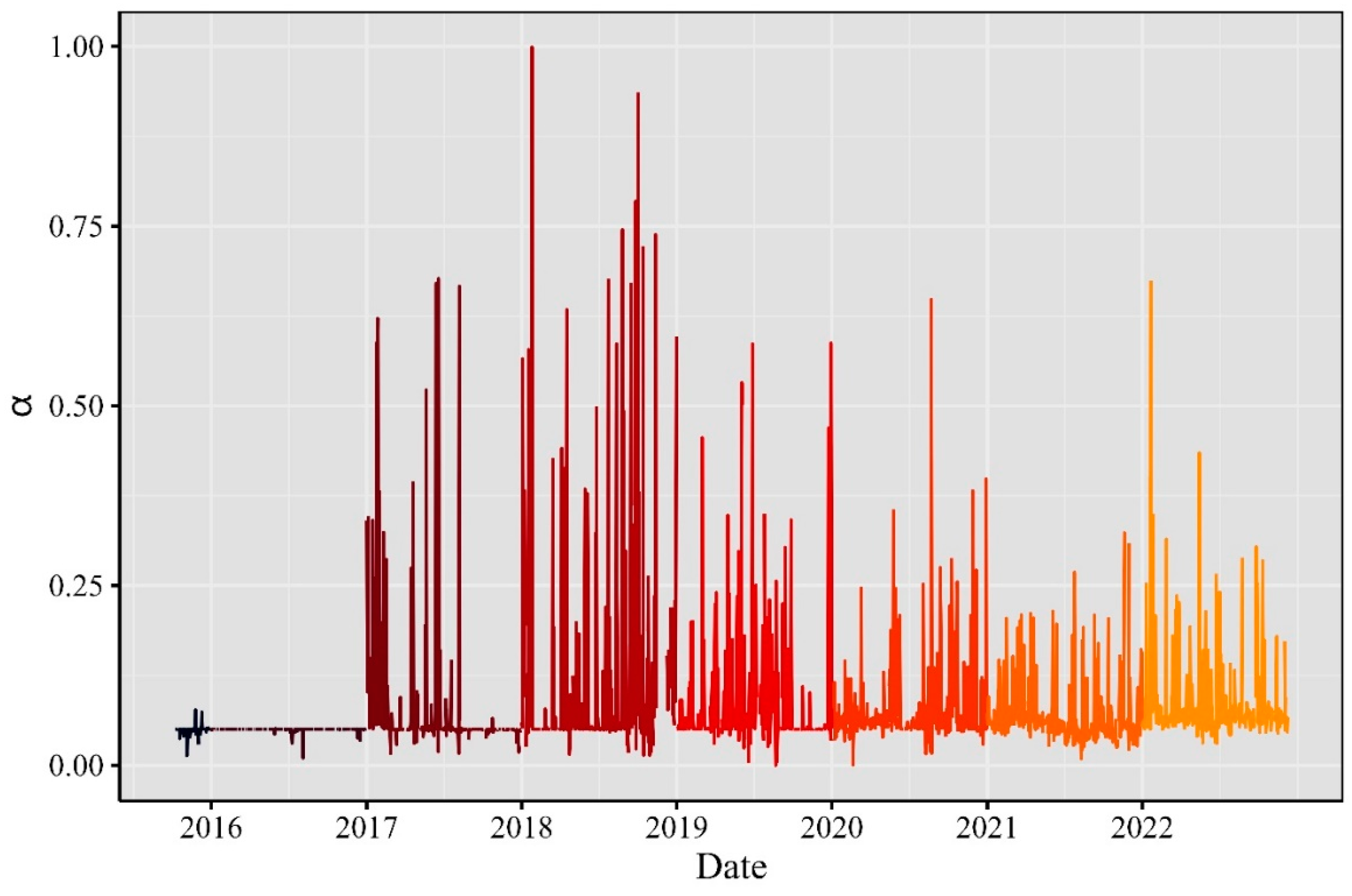
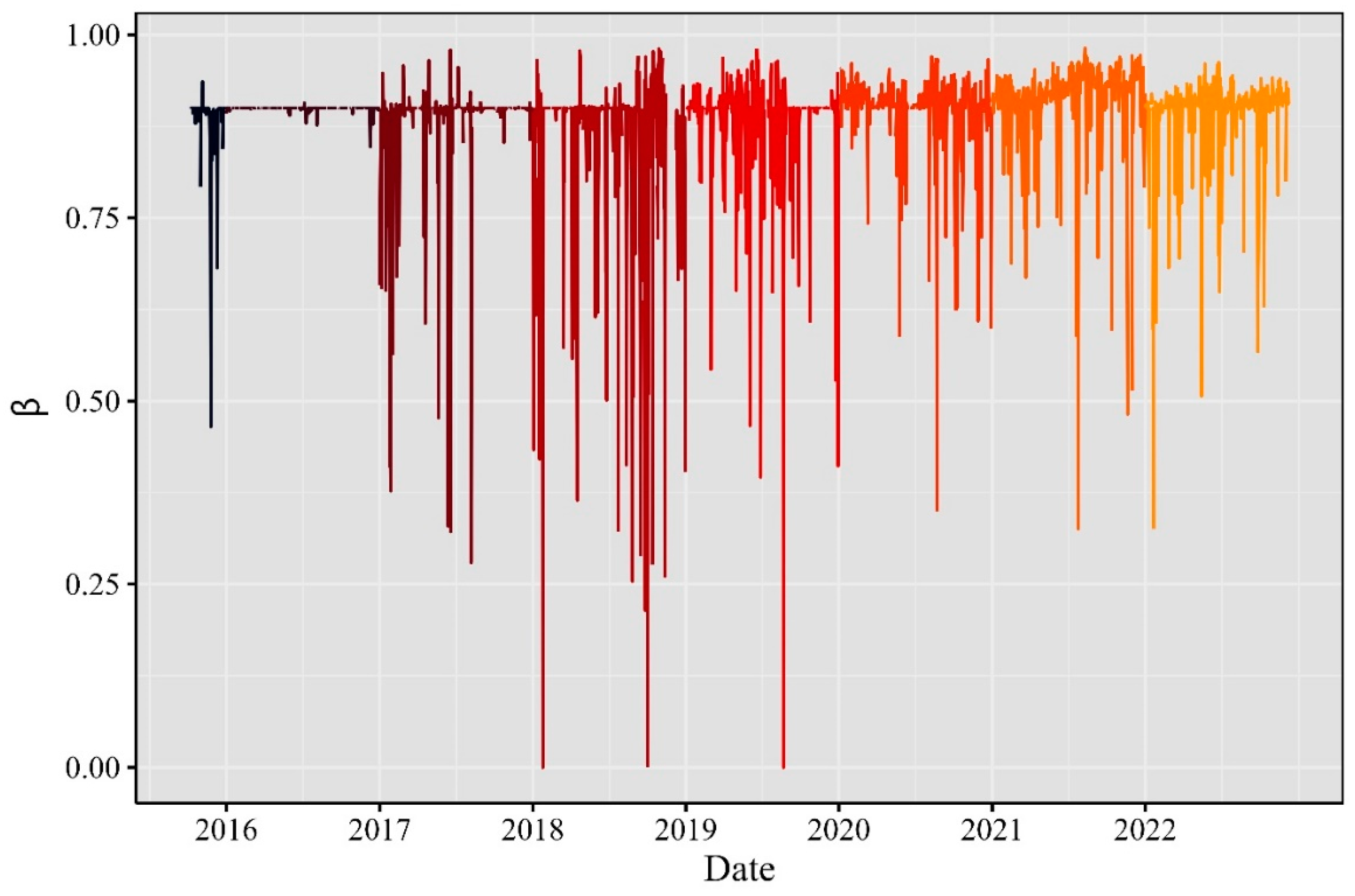
The parameters ω, α and β in Figure 3, Figure 4 and Figure 5, respectively, determine the variance equation of the GARCH(1,1) model. The coefficients were positive and their highest values were recorded in 2018 for α, and similar peaks for β were recorded in 2018 and 2019. Important variations can be seen throughout the observation period. As mentioned before, Bitcoin’s highest peaks are related to the existence of bubbles, as shown by Contreras-Valdez [65].

Most series presented positive skewness values with some negative peaks. However, during 2015 and 2016, the values were consistent almost every day. This behavior might indicate a lack of asset popularity. It is probable that only a few investors participated in the Bitcoin/Ethereum market during that period. Nevertheless, the estimator became more volatile in 2017, and again during 2018, and at some point, volatility created the previously reported financial bubble. The lowest points for this parameter corresponded to the final days of 2019 and the beginning of the pandemic.

Regarding the shape parameter, the estimated results showed more distinguishable behavior for the pre-2019 period. The peak in 2018 happened in November, just prior to the collapse of the financial bubble. The next peaks occurred during 2019. The most noticeable appeared in March 2020, and was associated with the beginning of the pandemic. During 2021, the peaks were exacerbated, like the previously described parameters, and they were dampened during 2022. During these last two years, some bubble episodes created the impression of extreme behavior in returns, such that the tails’ density was increased, particularly on the left side. This type of study can be valuable for risk-management purposes because it allows for the daily recalibration of strategies, especially during periods of turmoil.

Regarding the ETH/USD exchange rate, Figure 8, Figure 9, Figure 10, Figure 11, Figure 12, Figure 13 and Figure 14 present the GARCH models’ parameter estimations. As before, the values are grouped and colored by year.

Only one constant term was estimated for the ETH’s conditional mean equation. This expected value follows almost the same behavior as in the case of the BTC estimation where, most of the time, the values are close to zero, but with some peaks that closely resemble those of BTC, suggesting a high correlation between the two cryptocurrencies.

Regarding the risk premium estimator, its values are consistent with those for BTC. Only two peaks appear in the data for 2019. During 2021 and 2022, its behavior seems more homogeneous than for BTC, showing that, although the cryptocurrencies’ behaviors are very similar, some discrepancies can be detected that suggest where to invest.

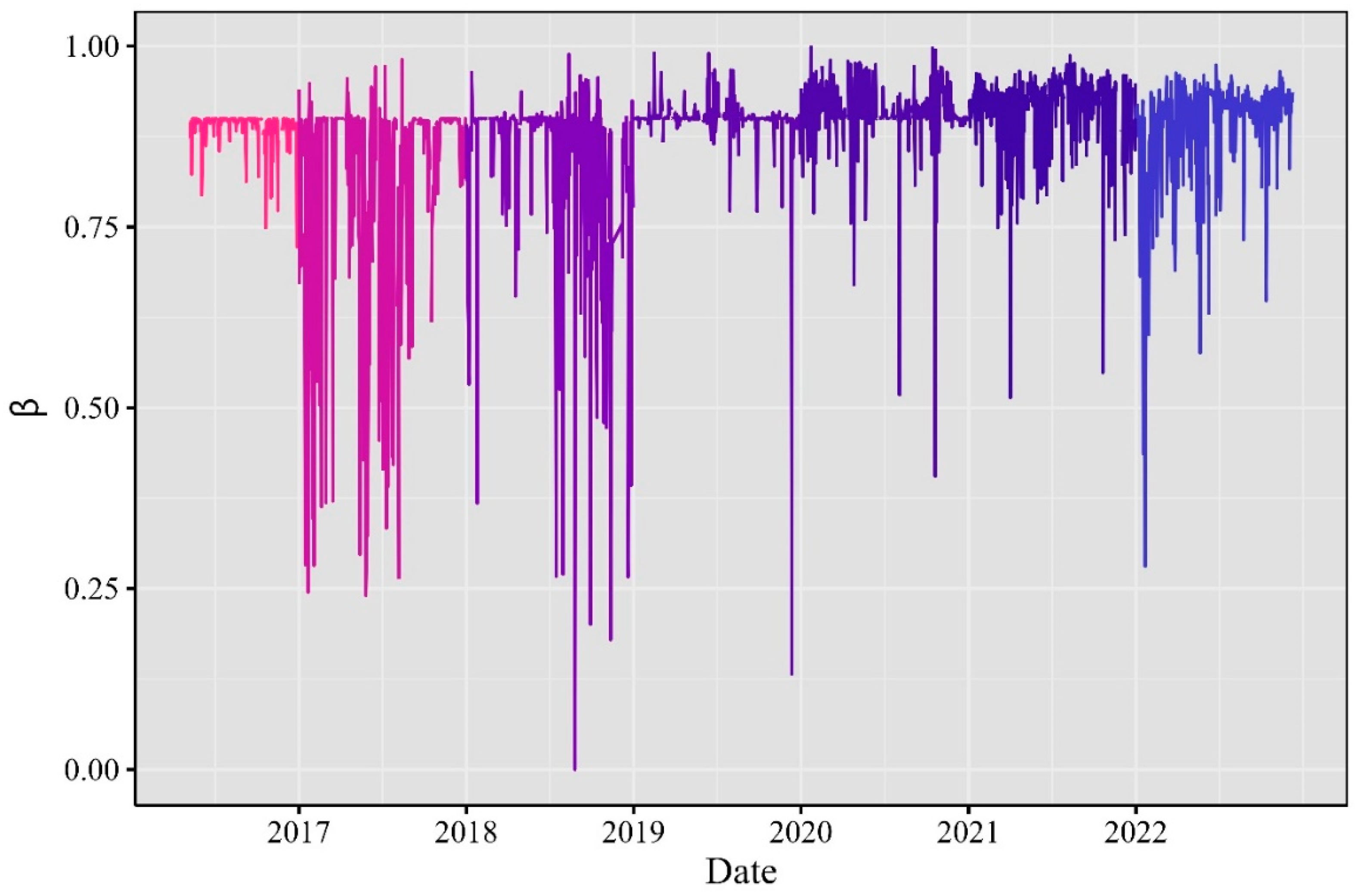
Similarly to the Bitcoin case, in Figure 10, Figure 11 and Figure 12, Ethereum had positive parameters in its GARCH(1,1) model variance equation. In the case of α, several similar peak values were present during 2018. In the case of β, there was a peak in 2018, consistent with the findings reported for the BTC market.

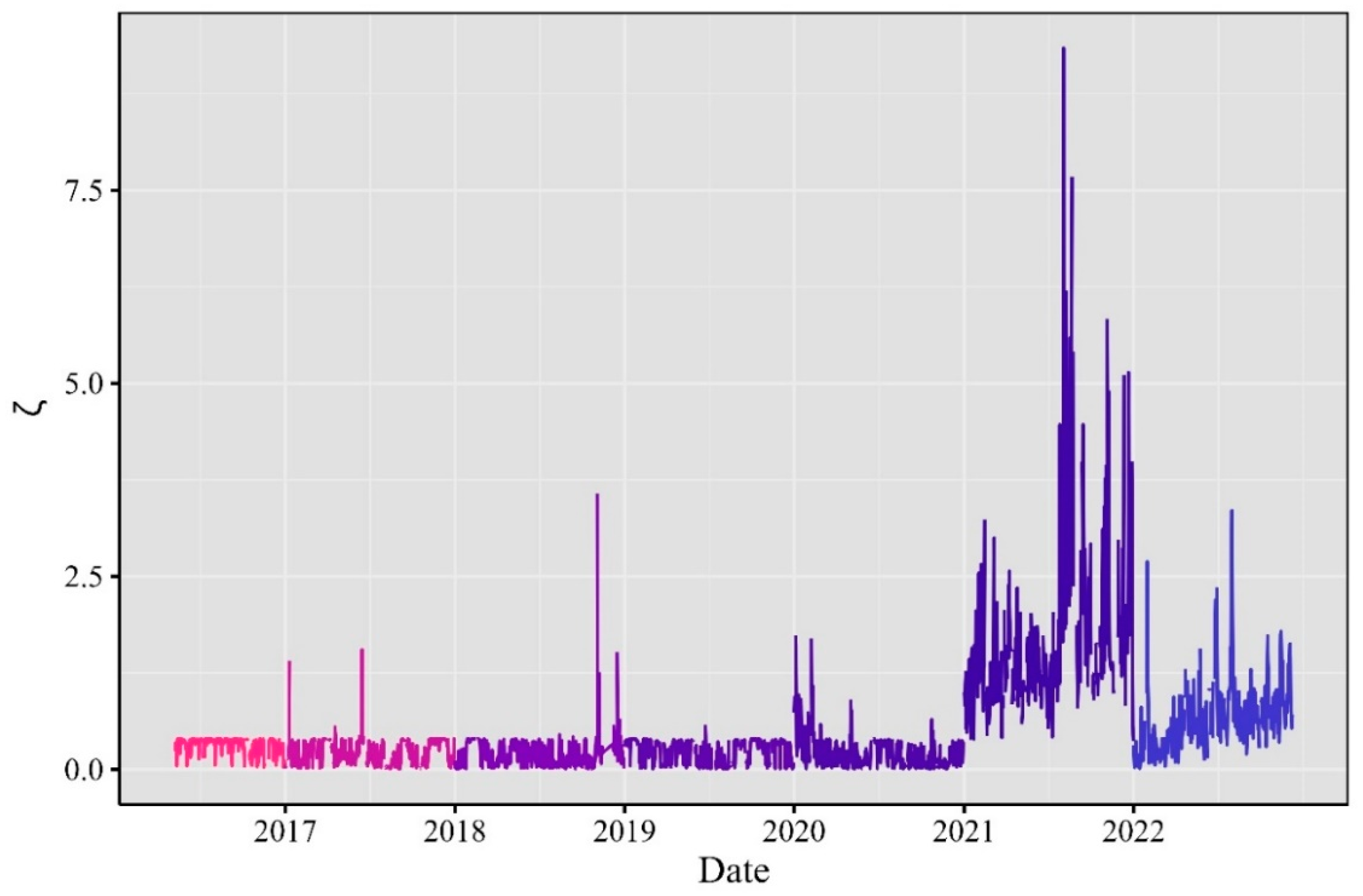
The skewness and shape estimators for both ETH and BTC had similar behavior. Regarding the shape coefficient, its values remained consistent until 2021. During that year, there was a large increment in the weight of the tails, which receded in 2022. As excess kurtosis reflects the presence of extreme returns values, 2022 should be studied in more depth to better understand the recorded bubble episodes. Regarding the skew, once more, the values tended to be positive, but in the last two years, this range was reduced to closer to zero. The evolution of the market’s pre- and post-pandemic periods seems to be complex enough to apply dynamic approaches to evaluate the behavior of returns.

5. Discussion

This research represents a departure from the widely used GARCH models in the literature on volatility (see, for example, Bariviera et al. [23], Katsiampa [24], Troster et al. [25], Catania et al. [44] and Chu et al. [48]) because it employs a GARCH model with residuals that have a Normal-Inverse Gaussian (NIG) distribution, like in Gyamerah [22].

A different GARCH model was estimated for every day of the observation period (i.e., 1440 estimations) using high-frequency (minute-by-minute) data; therefore, this paper also contributes to the literature on the tradeoff between risk and return for different indices using high-frequency data, in line with Baron et al. [12], Almeida et al. [13], Ji [14] and Pele et al. [16]. The methodological approach used to estimate the daily parameters provides more accurate support for decision makers because it allows for more continuous information flow and enables more timely adjustments to market participants’ strategies. The α and β parameters, whose addition indicates the persistence of volatility, allow for closer monitoring of the daily changes in the market.

One of the important findings of this study is that the parameters exhibited important variations throughout both the COVID-19 and the non-COVID-19 subperiods. Larger variations were not necessarily associated with the sanitary emergency, in contrast with the results reported by Salisu et al. [58].

Regarding the residuals’ distribution parameters, the NIG distribution is adequate for making adjustments, but the ρ and ζ parameters have important variability over time. Noticeably, during the 2021 and 2022 COVID-19 period, $\zeta$ reaches its greatest variation.

Models of volatility are of great importance in finance. There are numerous models that can be applied to data depending on the characteristics to be studied. The availability of minute-by-minute data has provided an opportunity to deliver more detailed analyses of the risk premium dynamics of the returns of BTC/USD and ETH/USD rates.

6. Conclusions

Based on our findings, we conclude that even though the COVID-19 pandemic period was characterized by intense turbulence in the financial markets, volatility led to larger variations during other periods. For example, regarding the dynamic evolution of risk premium, the greatest peak of this risk premium was observed in 2019, one year before the COVID-19 pandemic started. This highlights the importance of better understanding the volatility behavior and evolution of returns, which is crucial to the success of risk management and trading strategies implemented by practitioners.

In this study, we can observe the evolution over time of skewness and kurtosis given the parametrization of the NIG distribution used. Given the variability of these parameters, it is of interest to analyze arbitrage opportunities on a daily basis. Similarly, the typical parameters of a GARCH(1,1) model, which indicate the dependence on past variance and square errors, directly impact the predicted value via the variance equation. This can be used by risk managers to update different estimates, for example, value at risk (VaR) and conditional value at risk (CvaR).

The reported results resemble those of previous analyses on cryptocurrency bubble episodes. The highest values in the higher-order moments occur during the recorded bubble episodes of 2016 and 2018. By contrast, during the COVID-19 period, these values are less pronounced. Such behavior might be related to the microstructure of the market; as more people and institutions participated, the volume of transactions and the market’s capitalization might have undergone a smoother evolution. Further studies in this area are needed to determine the changes that took place in the market and the overall behavior of cryptocurrencies in this post-COVID-19 era.

Our modeling approach offers the possibility to compare different periods of turmoil, like the COVID-19 emergency and other market bubbles, therefore impacting the decisions of regulatory authorities when warning financial agents about the consequences of investing in the two main cryptocurrencies. Even for agents that do not have these cryptocurrencies, the consequences of strong movements in volatility are very clear in this deeply interrelated financial world. Having a tool to measure the day-to-day movements of these digital assets is very useful because we can use these estimations to feed simulations about what scenarios might occur. Changes in the regulation of these assets can be redefined in different ways to promote the stability of the financial system, as their nature can be better understood with the support of high-frequency data.

A limitation of our study is that it does not incorporate the detection of changes in the behavior of data, for example, the use of Markov switching GARCH (MSGARCH) models to detect changes in time series regimes and the probability of moving from one state to another. In future research, the use of MSGARCH can be used to detect changes in regimes with their associated matrix of probabilities. Additionally, we can estimate VaR and CVAR risk measures with daily periodicity based on high-frequency data.