A Flexible Extended Krylov Subspace Method for Approximating Markov Functions of Matrices

Abstract

A flexible extended Krylov subspace method ($\mathcal{F}$-EKSM) is considered for numerical approximation of the action of a matrix function $f\left(A\right)$ to a vector b, where the function f is of Markov type. $\mathcal{F}$-EKSM has the same framework as the extended Krylov subspace method (EKSM), replacing the zero pole in EKSM with a properly chosen fixed nonzero pole. For symmetric positive definite matrices, the optimal fixed pole is derived for $\mathcal{F}$-EKSM to achieve the lowest possible upper bound on the asymptotic convergence factor, which is lower than that of EKSM. The analysis is based on properties of Faber polynomials of A and ${(I-A/s)}^{-1}$. For large and sparse matrices that can be handled efficiently by LU factorizations, numerical experiments show that $\mathcal{F}$-EKSM and a variant of RKSM based on a small number of fixed poles outperform EKSM in both storage and runtime, and usually have advantages over adaptive RKSM in runtime.

1. Introduction

Consider a large square matrix $A\in {\mathbb{R}}^{n\times n}$ and a function f such that the matrix function $f\left(A\right)\in {\mathbb{R}}^{n\times n}$ is well-defined [1,2]. The numerical approximation of

$$q=f\left(A\right)b,$$

(1)

where $b\in {\mathbb{R}}^n$ is a vector, is a common problem in scientific computing. It arises in numerical solutions of differential equations [3,4,5,6], matrix functional integrators [7,8], model order reduction [9,10], and optimization problems [11,12]. Note that approximating the action of $f\left(A\right)$ to a vector b and approximating the matrix $f\left(A\right)$ are different. For a large sparse matrix A, $f\left(A\right)$ is usually fully dense and infeasible to form explicitly.

Numerical methods for approximating the action of $f\left(A\right)$ to a vector have been extensively studied in recent years, especially for large-scale problems; see, e.g., [13,14,15] and references therein. Existing algorithms often construct certain polynomial or rational approximations to f over the spectrum of A and apply such approximations directly to the vector b without forming any dense matrices of the same size as A. A class of mostly common projection methods are based on Krylov subspaces ${\mathcal{K}}_m(A,b)$; however, for many large matrices this may require a very large dimension of approximation spaces. Rational Krylov subspace methods have been investigated to decrease the size of subspaces for approximations; see, e.g., [16,17,18,19,20]. Two well-known examples are the extended rational Krylov subspace method (EKSM) [14,21,22] and the adaptive rational Krylov subspace method (adaptive RKSM) [23,24].

In this paper, we explore a generalization of EKSM that uses one fixed nonzero pole alternately with the infinite pole for approximating the action of Markov-type (Cauchy–Stieltjes) functions [25]. Markov-type functions can be written as

$$f\left(z\right)={\int }_{-\infty }^0\frac{d\mu \left(\zeta \right)}{z-\zeta },z\in \mathbb{C}\setminus (-\infty ,0],$$

where $\mu$ is a measure that ensures that the integral converges absolutely. Note that this definition can be generalized to integrals defined on $[\alpha ,\beta ]$, where $-\infty \le \alpha <\beta <\infty$. We consider the interval $(-\infty ,0]$ here, as this is sufficient for the most widely-studied Markov-type functions $f\left(z\right)=z^{\gamma }$ with $-1<\gamma <0$, $f\left(z\right)=\frac{e^{\theta \sqrt{z}}-1}{z}$ and for their simple modifications, such as $z^{\mathsf{\ell }}f\left(z\right)$ with $\mathsf{\ell }\in {\mathbb{Z}}^{+}$. Our analysis can be extended to integrals on $(-\infty ,\beta ]$ as long as the measure $\mu \left(\zeta \right)$ satisfies ${\int }_{-\infty }^{\beta }\left|d\mu \left(\zeta \right)\right|<\infty$, as assumed in [21].

This study is motivated by [21], which provided an upper bound on the convergence factor of EKSM for approximating $f\left(A\right)b$. Our work concerns a generalization of EKSM, replacing the zero pole used in EKSM with a fixed nonzero pole s; hence, we call it the flexible extended Krylov subspace method ($\mathcal{F}$-EKSM). This algorithm can apply the three-term recurrence to enlarge the subspace for symmetric matrices such as EKSM, while full orthogonalization process may be necessary for adaptive RKSM regardless of the symmetry of matrices. Beckermann and Reichel [26] studied the asymptotic convergence rate of RKSM with different pole selections for approximating $f\left(A\right)b$ of Markov functions via Faber transform; however, they did not provide explicit expressions of the optimal cyclic 2 poles or the corresponding rate of convergence, which could be done by solving a quartic equation analytically. In this paper, we derive explicit expressions of the optimal pole s and the corresponding convergence factor using the different analytic tool from [21]. While our bounds on the convergence factor seem to not be as tight as the bounds in [26] numerically, our poles and bounds are provided in explicit expressions; in addition, our pole usually leads to faster convergence for discrete Laplacian matrices based on finite difference discretizations and many practical nonsymmetric matrices.

We explore the optimal pole s to achieve the lowest upper bound on the asymptotic convergence factor, which is guaranteed to outperform EKSM on symmetric positive definite (SPD) matrices. For nonsymmetric matrices with an elliptic numerical range, we provide numerical evidence to demonstrate the advantage of $\mathcal{F}$-EKSM over EKSM in convergence rate. Numerical experiments show that $\mathcal{F}$-EKSM converges at least as rapidly as the upper bound suggests. In practice, if the linear systems needed for constructing rational Krylov subspaces can be solved efficiently by LU factorizations, then $\mathcal{F}$-EKSM outperforms EKSM in both time and storage cost over a wide range of matrices, and it could run considerably faster than adaptive RKSM for many problems. In this paper, we only consider factorization-based direct methods for solving the inner linear systems; for the use and implications of iterative linear solvers see, e.g., [27].

Rational Krylov subspace methods may exhibit superlinear convergence for approximating $f\left(A\right)b$. As the algorithms proceed and more rational Ritz values converge to the exterior eigenvalues of A, the ‘effective spectrum’ of A not covered by the converged Ritz values shrinks, leading to gradual acceleration of the convergence. This analysis has been performed for EKSM applied to the 1D discrete Laplacian ([28], Section 5.2) based on the result from [21], leading to a sharper explicit bound on the convergence. The same idea could be explored with $\mathcal{F}$-EKSM; however, it is not considered here, as we did not observe superlinear convergence in our experiments. This was probably because the effective spectrum of our large test matrices did not shrink quickly enough to exhibit convergence speedup before the stopping criterion was satisfied.

Though $\mathcal{F}$-EKSM is closely connected to EKSM, we emphasize that the convergence of $\mathcal{F}$-EKSM cannot be derived directly from that of EKSM applied to a shifted matrix. Admittedly, with the same vector b it is the case that $\mathcal{F}$-EKSM with a pole s applied to A and EKSM applied to $I-A/s$ both generate the same subspaces ${\mathcal{Q}}_{2m+1}^{\left(s\right)}(A,b)={(I-A/s)}^{-m}\mathrm{span}\{b,Ab,...,A^{2m}b\}$, however, the existing theory of EKSM [21] can only provide a bound on the convergence factor for approximating $f(I-A/s)b$, which is not what is needed and has no obvious relationship with the convergence for approximating $f\left(A\right)b$ from the same subspace. Our analysis is based on a special min–min optimization instead of the results of EKSM applied to a shifted matrix.

The remainder of this paper is organized as follows. In Section 3, we discuss the implementation of $\mathcal{F}$-EKSM. In Section 4, we analyze the linear convergence factor of $\mathcal{F}$-EKSM and provide the optimal pole with which the lowest upper bound on the convergence factor can be achieved for SPD matrices. In addition, we numerically explore the optimal pole and the convergence factor of $\mathcal{F}$-EKSM for nonsymmetric matrices with an elliptic numerical range. In Section 5, we consider a variant of RKSM that applies a few fixed cyclic poles to provide faster approximations than $\mathcal{F}$-EKSM for certain challenging nonsymmetric matrices. In Section 6, we show the results of numerical experiments for different methods on a variety of matrices. Our conclusions are provided in Section 7, followed by several proofs of Lemmas in the Appendices.

2. Rational Krylov Subspace Methods and $\mathcal{F}$-EKSM

For a wide range of matrix function approximation problems, polynomial Krylov subspace methods converge very slowly [29,30]. To speed up convergence, a more efficient approach is to apply rational Krylov subspace methods; see, e.g., [31,32] and references therein.

The procedure of RKSM is outlined as follows. Starting with an initial nonzero vector b that generates ${\mathcal{Q}}_1(A,b)=\mathrm{span}\left\{v_1\right\}$, where $v_1=b/\left|\right|b\left|\right|$, RKSM keeps expanding the subspaces to search for increasingly more accurate approximate solutions to our problem of interest. In order for RKSM to expand the current subspace ${\mathcal{Q}}_m(A,b)$ to ${\mathcal{Q}}_{m+1}(A,b)$, we apply the linear operator ${({\gamma }_{m}I-{\eta }_{m}A)}^{-1}({\alpha }_{m}I-{\beta }_{m}A)$ to a vector $u\in {\mathcal{Q}}_m(A,b)\setminus {\mathcal{Q}}_{m-1}(A,b)$. To build an orthonormal basis $\{v_1,v_2,...,v_{m+1}\}$ of the enlarged subspace ${\mathcal{Q}}_{m+1}(A,b)$, we may choose $u=v_m$ and adopt the modified Gram–Schmidt orthogonalization, obtaining

$${({\gamma }_{m}I-{\eta }_{m}A)}^{-1}({\alpha }_{m}I-{\beta }_{m}A)v_m={\sum }_{i=1}^{m+1}{h}_{im}{v}_i,$$

(2)

where $h_{im}=v_i^{*}{({\gamma }_{m}I-{\eta }_{m}A)}^{-1}({\alpha }_{m}I-{\beta }_{m}A)v_m$. To ensure that the linear operator is well-defined and nonsingular, we require that $|{\gamma }_m{|}^2+{\left|{\eta }_m\right|}^2\ne 0$, $|{\alpha }_m{|}^2+{\left|{\beta }_m\right|}^2\ne 0$, $({\gamma }_m,{\eta }_m)\ne ({\alpha }_m,{\beta }_m)$ up to a scaling factor, and that $\frac{{\alpha }_m}{{\beta }_m}$ and $\frac{{\gamma }_m}{{\eta }_m}$ (if ${\beta }_m$ and ${\eta }_m$ are nonzeros) not be an eigenvalue of A. The use of four parameters (${\alpha }_m,{\beta }_m,{\gamma }_m,{\eta }_m$) provides the flexibility to accommodate both the zero (${\gamma }_m=0$, ${\eta }_m=-1$) and the infinity (${\gamma }_m=1$, ${\eta }_m=0$) poles in a unified framework. The expansion of rational Krylov subspaces does not have to be based on the last orthonormal basis vector $u=v_m$, as in (2). There are alternative ways to choose the continuation vector to expand the subspaces; see, e.g., [33].

The shift-inverse matrix vector product ${({\gamma }_{m}I-{\eta }_{m}A)}^{-1}({\alpha }_{m}I-{\beta }_{m}A)v_m$ is equivalent to solving $({\gamma }_{m}I-{\eta }_{m}A)w=({\alpha }_{m}I-{\beta }_{m}A)v_m$ (the inner linear system) for w. Multiplying both sides of (2) by ${\gamma }_{m}I-{\eta }_{m}A$, moving all terms containing A to the left-hand side and all other terms to the right-hand side, we have

$$A\left({\sum }_{i=1}^{m+1}{\eta }_m{h}_{im}{v}_i-{\beta }_m{v}_m\right)=-{\alpha }_m{v}_m+{\gamma }_m{\sum }_{i=1}^{m+1}{h}_{im}{v}_i.$$

(3)

Note that the above relation should hold for each index value $m=1,2,...$, thus, it is not hard to see that (3) can be written in the following matrix form:

$$\begin{array}{cc}\hfill A{V}_{m+1}{\underline{F}}_m& \equiv A{V}_{m+1}\left({\underline{H}}_m\mathrm{diag}({\eta }_1,\dots ,{\eta }_m)-\left[\begin{array}{c}\mathrm{diag}({\beta }_1,\dots ,{\beta }_m)\\ 0_{1\times m}\end{array}\right]\right)\hfill \\ \hfill & =V_{m+1}\left({\underline{H}}_m\mathrm{diag}({\gamma }_1,\dots ,{\gamma }_m)-\left[\begin{array}{c}\mathrm{diag}({\alpha }_1,\dots ,{\alpha }_m)\\ 0_{1\times m}\end{array}\right]\right)\equiv V_{m+1}{\underline{G}}_m,\hfill \end{array}$$

where $V_{m+1}=\left[v_1,v_2,...,v_{m+1}\right]$ contains the orthonormal basis vectors of the rational Krylov subspace:

$$\begin{array}{ccc}& & {\mathcal{Q}}_{m+1}\left(A,v_1\right)=q_m{\left(A\right)}^{-1}{\mathcal{K}}_{m+1}\left(A,v_1\right)\hfill \\ & =& \left(\prod _{k=1}^m{({\gamma }_{k}I-{\eta }_{k}A)}^{-1}\right)\mathrm{span}\left\{v_1,A{v}_1,A^2{v}_1,...,A^m{v}_1\right\},\hfill \end{array}$$

and ${\underline{H}}_m$, ${\underline{F}}_m$, and ${\underline{G}}_m\in {\mathbb{R}}^{(m+1)\times m}$ are all upper Hessenberg matrices. Specifically,

$$\begin{array}{cc}\hfill {\underline{H}}_m=\left[\begin{array}{c}{H}_m\\ h_{(m+1)m}{e}_m^{*}\end{array}\right],{\underline{F}}_m& =\left[\begin{array}{c}{F}_m\\ f_{(m+1)m}{e}_m^{*}\end{array}\right]=\left[\begin{array}{c}{H}_m\mathrm{diag}({\eta }_1,...,{\eta }_m)-\mathrm{diag}({\beta }_1,...,{\beta }_m)\\ h_{(m+1)m}{\eta }_m{e}_m^{*}\end{array}\right],\hfill \\ \hfill {\underline{G}}_m& =\left[\begin{array}{c}{G}_m\\ g_{(m+1)m}{e}_m^{*}\end{array}\right]=\left[\begin{array}{c}{H}_m\mathrm{diag}({\gamma }_1,...,{\gamma }_m)-\mathrm{diag}({\alpha }_1,...,{\alpha }_m)\\ h_{(m+1)m}{\gamma }_m{e}_m^{*}\end{array}\right],\hfill \end{array}$$

(4)

where $e_m={[0,\dots ,0,1]}^{*}\in {\mathbb{R}}^m$.

The idea of RKSM as a projection method is the same as standard Krylov: first, solve the Galerkin projected problem defined for $V_m^{*}A{V}_m=F_m{G}_m^{-1}$, then project the solution back to the m-dimensional subspace as an approximate solution for the original problem defined for A.

The parameters ${\alpha }_m,{\beta }_m,{\gamma }_m,{\eta }_m$ can be changed in each iteration to determine the poles. For example, if we set ${\alpha }_k={\eta }_k=0$,${\gamma }_k=1$ and ${\beta }_k=-1$ for all $k\in {\mathbb{Z}}^{+}$, it is the standard Krylov subspace method; if we set ${\beta }_{2k}={\eta }_{2k-1}=-1$, ${\alpha }_{2k-1}={\gamma }_{2k}=1$, and ${\alpha }_{2k}={\beta }_{2k-1}={\gamma }_{2k-1}={\eta }_{2k}=0$ for $k\in {\mathbb{Z}}^{+}$, it becomes EKSM. A special variant of EKSM [34,35] constructs the following extended subspaces:

$${\mathcal{K}}^{l,m}(A,b)=\mathrm{span}\left\{A^{-l+1}b,...,A^{-1}b,b,Ab,...,A^{m-1}b\right\}.$$

(5)

A practical choice for the two indices l and m leads to subspaces of the form ${\mathcal{K}}^{m,im+1}(A,b)$ for some $i\in {\mathbb{N}}^{+}$, which requires an orthonormal basis for the Krylov subspaces with vectors

$$b,Ab,A^{2}b,...,A^{i}b,A^{-1}b,A^{i+1}b,...,A^{2i}b,A^{-2}b,A^{2i+1}b,....$$

However, there is no convergence theory for this special variant.

The general rational Krylov space of order m is provided by [36,37]:

$$\begin{array}{cc}\hfill {\mathcal{Q}}_m(A,b)& =q_{m-1}{\left(A\right)}^{-1}\mathrm{span}\{b,Ab,...,A^{m-1}b\},\hfill \\ \hfill \mathrm{where}{q}_{m-1}\left(z\right)& =({\gamma }_1-{\eta }_{1}z)({\gamma }_2-{\eta }_{2}z)...({\gamma }_{m-1}-{\eta }_{m-1}z),\hfill \end{array}$$

with ${\gamma }_i,{\eta }_i$ prescribed in (2). For EKSM, the rational Krylov subspace of dimension is

$$\begin{array}{cc}\hfill {\mathcal{Q}}_{2m+1}^{\left(E\right)}(A,b)& ={\mathcal{K}}_{m+1}(A,b)\cup {\mathcal{K}}_{m+1}(A^{-1},b)=A^{-m}\mathrm{span}\left\{b,Ab,...,A^{2m}b\right\}.\hfill \end{array}$$

EKSM applies the operators $A^{-1}$ and A in an alternating manner in each iteration.

For adaptive RKSM, the operation at step m can be written as follows:

$${(I-A/s_m)}^{-1}(A-{\sigma }_{m}I)v_m={\sum }_{i=1}^{m+1}{h}_{im}{v}_i,$$

where $s_m$ is a nonzero pole and ${\sigma }_m$ is a zero of the underlying rational function. To find the optimal poles and zeros at each step, we first restrict the poles and zeros to disjoint sets $\Xi$ and $\Sigma$, respectively, where $\Sigma \supseteq W\left(A\right)$ and $\Xi \subseteq \mathbb{C}\setminus W\left(A\right)$[38] and where $W\left(A\right)=\left\{x^{*}Ax|x\in {\mathbb{C}}^n,{\parallel x\parallel }_2=1\right\}$ is the numerical range of A. The pair $(\Sigma ,\Xi )$ is called a condenser [39,40]. An analysis of RKSM considers a sequence of rational nodal functions

$$r_m\left(z\right)={\prod }_{j=1}^m\frac{z-{\sigma }_j}{1-z/s_j},$$

where the zeros ${\sigma }_j\in \Sigma$ and the poles $s_j\in \Xi$. Adaptive RKSM tries to obtain asymptotically optimal rational functions by defining ${\sigma }_{j+1}$ and $s_{j+1}$ recursively with the following conditions: after choosing ${\sigma }_1$ and $s_1$ of minimal distance, define [38]:

$${\sigma }_{j+1}=arg\underset{z\in \Sigma }{max}\left|r_j\left(z\right)\right|,s_{j+1}=arg\underset{z\in \Xi }{min}\left|r_j\left(z\right)\right|.$$

(6)

The points $\left\{({\sigma }_j,s_j)\right\}$ are called generalized Leja points [41,42]. In practice, we compute approximations with respect to the poles and zeros defined in (6) during the progress of iteration. Adaptive RKSM usually converges with fewer iterations than EKSM while using a smaller approximation subspace [24,38,43]. While usually converging in fewer iterations than the variants with a few cyclic poles [32], each step of adaptive RKSM requires a solution to a shifted linear system with a new shift, which is more expensive than using existing LU factorizations to solve the linear system with the same coefficient matrix that has been factorized. If the linear system at each RKSM step is solved by a direct method, adaptive RKSM tends to require longer runtimes than variants with a few cyclic poles based on reusing LU factorizations for each distinct pole. Adaptive RKSM is most competitive if the linear systems arising from each step need to be solved approximately by an iterative method and if effective preconditioning can be structured for each linear system with different shift.

In this paper, we consider generating rational Krylov subspaces with cyclic poles s, $+\infty$, s, $+\infty$, $...$ ($s\ne 0$), which we call the flexible extended Krylov subspace method ($\mathcal{F}$-EKSM). The corresponding linear operators are provided by ${(I-A/s)}^{-1}$ and A, which are applied in an alternating manner. To this end, we set ${\beta }_{2k}=-1$, ${\eta }_{2k-1}=1/s$, ${\alpha }_{2k-1}={\gamma }_k=1$, and ${\alpha }_{2k}={\beta }_{2k-1}={\eta }_{2k}=0$ for $k\in {\mathbb{Z}}^{+}$. The approximation space of $\mathcal{F}$-EKSM is

$${\mathcal{Q}}_{2m+1}^{\left(s\right)}(A,b)={(I-A/s)}^{-m}\mathrm{span}\{b,Ab,...,A^{2m}b\}.$$

The choice of the repeated pole s influences the convergence rate of $\mathcal{F}$-EKSM. Our goal is to find the optimal pole $s^{*}$ for Markov-type functions of matrices such that $\mathcal{F}$-EKSM achieves the lowest upper bound on the linear convergence factor. This subspace is identical to the one generated by EKSM applied to the shifted matrix $I-A/s$; the convergence theory of EKSM [21] would provide a convergence factor bound for approximating $f(I-A/s)b$ instead of $f\left(A\right)b$, however, this is not our concern here, as our results are derived with a special min–min optimization analysis, not from the results of EKSM applied to a shifted matrix.

3. Implementation of $\mathcal{F}$-EKSM for Approximating $\mathit{f}\left(\mathit{A}\right)\mathit{b}$

Without loss of generality, suppose that ${\left|\right|b\left|\right|}_2=1$ in (1) and let the initial subspace be $\mathrm{span}\left\{b,{(I-A/s)}^{-1}b\right\}$. The approximation to $f\left(A\right)b$ after $(m-1)$ steps is

$$q_m=V_{2m}f\left(A_m\right)V_{2m}^{*}b=V_{2m}f\left(A_m\right)e_1,$$

where $V_{2m}\in {\mathbb{C}}^{n\times \left(2m\right)}$ is an orthonormal set of basis vectors of the subspace

$${\mathcal{Q}}_{2m+1}^{\left(s\right)}(A,b)={\mathcal{K}}_m(A,b)\cup {\mathcal{K}}_m({(I-A/s)}^{-1},{(I-A/s)}^{-1}b)$$

and $A_m=V_{2m}^{*}A{V}_{2m}$ denotes the restriction of matrix A in ${\mathcal{Q}}_{2m+1}^{\left(s\right)}(A,b)$.

Because ${\mathcal{K}}_m(A,b)={\mathcal{K}}_m((I-A/s),b)$, we have ${\mathcal{Q}}_{2m+1}^{\left(s\right)}(A,b)={\mathcal{Q}}_{2m+1}^{\left(E\right)}(I-A/s,b)$. To construct this subspace, we can apply EKSM to the matrix $I-A/s$, obtain $V_{2m}=\left[v_1,...,v_{2m}\right]$ as the orthonormal set of basis vectors of ${\mathcal{Q}}_{2m+1}^{\left(E\right)}(I-A/s,b)$, and obtain

$${\mathcal{T}}_{2m}=V_{2m}^{*}(I-A/s)V_{2m}\in {\mathbb{R}}^{2m\times 2m},$$

(7)

which is a block upper Hessenberg matrix (see Section 3 in [22]). From (7), we obtain $A_m=V_{2m}^{*}A{V}_{2m}=s(I_{2m}-{\mathcal{T}}_{2m})$. Following the derivation of EKSM [22], we can derive a similar Arnoldi relation $A{V}_{2m}=V_{2m+2}{\underline{T}}_{2m}$ for our proposed $\mathcal{F}$-EKSM, where ${\underline{T}}_{2m}\in {\mathbb{R}}^{(2m+2)\times 2m}$ is a block upper Hessenberg matrix with $2\times 2$ blocks, and we obtain $A_m=V_{2m}^{*}A{V}_{2m}=T_{2m}$. More implementation details of RKSM can be found in [33,44]. Notice that similar to EKSM, for symmetric problems, the orthogonalization cost of $\mathcal{F}$-EKSM can be saved with the block three-term recurrence to enlarge the subspace.

The residual norm of $\mathcal{F}$-EKSM is $∥f\left(A\right)b-V_{2m}f\left(A_m\right)e_1∥$; however, it is not directly computable because $f\left(A\right)b$ is unknown. One stopping criterion for the Arnoldi approximation is to compute $\left|h_{m+1,m}{e}_m^{*}f\left(A_m\right)e_1\right|$[30,45,46]; however, this may not be valid for RKSM. Another possibility is to compute $∥q_m-q_{m-1}∥$, which is the norm of the difference between two computed approximations; see, e.g., [21,47]. Alternatively, it is possible to monitor the angle $\angle (q_m,q_{m-1})$ between the approximations [48] in two consecutive iterations. This convergence criterion is sometimes used in the literature on eigenvalue computations; see, e.g., [49,50]. The two criteria usually exhibit very similar behavior. In this section, we choose the latter.

For all RKSM, linear system solvers are required in common, as the action of ${({\gamma }_{m}I-{\eta }_{m}A)}^{-1}$ to vectors is needed in (2). For EKSM and $\mathcal{F}$-EKSM, respectively, we need the action of $A^{-1}$ and ${(I-A/s)}^{-1}$ to the vectors. If these linear systems can be solved efficiently by direct methods, both of them need only one LU factorization performed one time and applicable to all linear solves. However, because of the adaptive poles, for adaptive RKSM it is necessary to solve a linear system with a different coefficient matrix for every iteration. Although adaptive RKSM achieves an asymptotically optimal convergence rate, it can be more time-consuming than EKSM and $\mathcal{F}$-EKSM, as a new LU factorization in each step is usually much more expensive than a linear solution using existing LU factors.

4. Convergence Analysis of $\mathcal{F}$-EKSM

Next, we study the optimal pole s for $\mathcal{F}$-EKSM to achieve the lowest upper bound on the convergence factor through min–min optimization.

4.1. General Convergence Analysis

In this section, we explore the asymptotic convergence of $\mathcal{F}$-EKSM. Consider the class of Markov-type functions $f\left(z\right)$ in (8). For any $a\ge 0$, a Markov-type function can be split into the sum of two integrals [14]:

$$\begin{array}{cc}\hfill f\left(z\right)& ={\int }_{-\infty }^0\frac{d\mu \left(\zeta \right)}{z-\zeta },z\in \mathbb{C}\setminus (-\infty ,0],\hfill \end{array}$$

(8)

$$\begin{array}{cc}\hfill f\left(z\right)& =f_1\left(z\right)+f_2\left(z\right),\mathrm{where}{f}_1\left(z\right)={\int }_{-\infty }^{-a}\frac{d\mu \left(\zeta \right)}{z-\zeta },f_2\left(z\right)={\int }_{-a}^0\frac{d\mu \left(\zeta \right)}{z-\zeta }.\hfill \end{array}$$

(9)

Here, we let $W_1:=W\left(A\right)=\{w^{*}Aw:{∥w∥}_2=1\}$ be the numerical range of matrix A and define $W_2:=\left\{\frac{s}{z-s}\right|z\in W_1\}$, where s is the repeated pole for $\mathcal{F}$-EKSM. We assume that $W_1$ is symmetric with respect to the real axis $\mathbb{R}$ and lies strictly in the right half of the complex plane. Then, for $s<0$, $W_2$ is symmetric with respect to the real axis $\mathbb{R}$ and lies in the left half of the complex plane. We define ${\varphi }_i:\overline{\mathbb{C}}\setminus W_i\to \overline{\mathbb{C}}\setminus D$ as the direct Riemann mapping [51] for $W_i$ ($i=1,2$), where D is the unit disk, and define ${\psi }_i={\varphi }_i^{-1}$ as the inverse Riemann mapping.

Our convergence analysis initially follows the approach in [21], then analyzes a special min–min optimization. It first uses the Faber polynomials [52], providing a rational expansion of functions for investigating the approximation behavior of $\mathcal{F}$-EKSM. The main challenge is to find how the fixed real pole s impacts the convergence and to determine the optimal s to achieve the lowest upper bound on the convergence factor.

Lemma 1.

For the Markov-type function defined by (8) (where μ is a measure such that the integral converges absolutely) and some given $a>0$, the following inequalities hold for any $m\in \mathbb{N},m>1$:

$$\begin{array}{ccc}\hfill \left|f_1\left(z\right)-\sum _{k=0}^{m-1}{\gamma }_{1,k}{F}_{1,k}\left(z\right)\right|& \le c_1{\left|{\varphi }_1(-a)\right|}^{-m},\hfill & \hfill z\in W_1,\end{array}$$

(10)

$$\begin{array}{ccc}\hfill \left|f_2\left(z\right)-\sum _{k=0}^{m-1}{\gamma }_{2,k}{F}_{2,k}\left(\frac{1}{z/s-1}\right)\right|& \le c_2{\left|{\varphi }_2\left(z_0\right)\right|}^{-m},\hfill & \hfill z\in W_1,\end{array}$$

(11)

where $|{\varphi }_2\left(z_0\right)|=min\left\{|{\varphi }_2(-1)|,\left|{\varphi }_2\left(\frac{s}{-a-s}\right)\right|\right\}$ and where $\left|{\varphi }_1(-a)\right|$, $\left|{\varphi }_2(-1)\right|$, and $\left|{\varphi }_2\left(\frac{s}{-a-s}\right)\right|$ are all greater than 1. Here, for $i=1,2$, ${\gamma }_{i,k}$ are some real numbers and $F_{i,k}$ denotes the Faber polynomials of degree k associated with the Riemann mapping ${\varphi }_i$, while $c_1$ and $c_2$ are constant positive real numbers independent of m.

Proof. 

The proof is provided in Appendix A.   □

Lemma 2.

Assume that ${\parallel b\parallel }_2=1$. For any given $a\ge 0$ used in (9), the error of approximating $f\left(A\right)b$ by $\mathcal{F}$-EKSM with cyclic poles s, $+\infty$, s, $+\infty$, $...$ satisfies

$$\parallel f\left(A\right)b-V_{2m}f\left(A_m\right)e_1\parallel \le c_{8}min{\left\{\left|{\varphi }_1(-a)\right|,\left|{\varphi }_2(-1)\right|,\left|{\varphi }_2\left(\frac{s}{-a-s}\right)\right|\right\}}^{-m}.$$

Proof. 

Let us define

$$g\left(z\right)=f_1\left(z\right)-\sum _{k=0}^{m-1}{\gamma }_{1,k}{F}_{1,k}\left(z\right),h\left(z\right)=f_2\left(z\right)-\sum _{k=0}^m{\gamma }_{2,k}{F}_{2,k}\left(\frac{1}{z/s-1}\right).$$

Because both g and h are analytic in $W_1$, and as $W\left(T_{2m}\right)\subset W_1$, from Theorem 2 in [53] we have

$$∥g\left(A\right)∥,∥g\left(A_m\right)∥\le 11.08\underset{z\in W_1}{max}\left|g\left(z\right)\right|,∥h\left(A\right)∥,∥h\left(A_m\right)∥\le 11.08\underset{z\in W_1}{max}\left|h\left(z\right)\right|.$$

Next, we follow the proof in Section 3, Theorem 3.4 in [21], and use the above inequality:

$$\begin{array}{cc}\hfill & \parallel f\left(A\right)b-V_{2m}f\left(A_m\right)e_1\parallel =\parallel f_1\left(A\right)b-{\sum }_{k=0}^{m-1}{\gamma }_{1,k}{F}_{1,k}\left(A\right)b-V_{2m}{f}_1\left(A_m\right)e_1\hfill \\ \hfill & +V_{2m}{\sum }_{k=0}^{m-1}{\gamma }_{1,k}{F}_{1,k}\left(A_m\right)e_1+f_2\left(A\right)b-{\sum }_{k=0}^m{\gamma }_{2,k}{F}_{2,k}\left(s{\left(A-sI\right)}^{-1}\right)b\hfill \\ \hfill & -V_{2m}{f}_2\left(A_m\right)e_1+V_{2m}{\sum }_{k=0}^m{\gamma }_{2,k}{F}_{2,k}\left(s{\left(A_m-sI\right)}^{-1}\right)e_1\parallel \hfill \\ \hfill =& ∥g\left(A\right)b-V_{2m}g\left(A_m\right)e_1+h\left(A\right)b-V_{2m}h\left(A_m\right)e_1∥\hfill \\ \hfill \le & \parallel g\left(A\right)\parallel +\parallel g\left(A_m\right)\parallel +\parallel h\left(A\right)\parallel +\parallel h\left(A_m\right)\parallel \hfill \\ \hfill \le & 2\times 11.08\left(\underset{z\in W_1}{max}\left|g\left(z\right)\right|+\underset{z\in W_1}{max}\left|h\left(z\right)\right|\right)\hfill \\ \hfill \le & 22.16\left(c_1{\left|{\varphi }_1(-a)\right|}^{-m}+c_{2}min{\left\{\left|{\varphi }_2(-1)\right|,\left|{\varphi }_2\left(\frac{s}{-a-s}\right)\right|\right\}}^{-m}\right)\hfill \\ \hfill \le & c_{8}min{\left\{\left|{\varphi }_1(-a)\right|,\left|{\varphi }_2(-1)\right|,\left|{\varphi }_2\left(\frac{s}{-a-s}\right)\right|\right\}}^{-m}.\hfill \end{array}$$

□

Remark 1.

The results of our analysis can additionally be applied to a linear combination of several Markov-type functions with monomials $z^l$, $l\in {\mathbb{Z}}^{+}$. One example of these functions is $f\left(z\right)=z^{\nu }$, $\nu \in (0,1)$, as $z^{\nu }=z{z}^{\nu -1}$ and $z^{\nu -1}$ is a Markov function. In addition, if the support of the underlying measure of the Markov function is a proper subset of $(-\infty ,0]$, the error bound may not be sharp. The asymptotic convergence might be superlinear as well; see, e.g., [28]. While this idea could be explored with $\mathcal{F}$-EKSM, it is not considered here because we did not observe superlinear convergence in our experiments. This was probably because the effective spectrum of our large test matrices did not shrink quickly enough to exhibit convergence speedup before the stopping criterion was satisfied.

To find the optimal pole to achieve the lowest upper bound on the asymptotic convergence factor of $\mathcal{F}$-EKSM, we need to determine $s\le 0$ such that

$$min\left\{\left|{\varphi }_1(-a)\right|,\left|{\varphi }_2(-1)\right|,\left|{\varphi }_2\left(\frac{s}{-a-s}\right)\right|\right\}$$

is maximized. Let us define

$$\rho (s,a)=1/min\left\{\left|{\varphi }_1(-a)\right|,\left|{\varphi }_2(-1)\right|,\left|{\varphi }_2\left(\frac{s}{-a-s}\right)\right|\right\}.$$

(12)

Therefore, $\mathcal{F}$-EKSM converges at least linearly with a convergence factor $\rho (s,a)<1$, where $\rho$ depends on s and a. For any given pole $s\le 0$, we can find the artificial parameter $a>0$ used in (9) such that it minimizes $\rho (s,a)$. Let $\tilde{\rho }\left(s\right)$ be the minimized $\rho (s,a)$; then, we need to find $s\le 0$ that minimizes $\tilde{\rho }\left(s\right)$. We denote the minimized $\tilde{\rho }\left(s\right)$ by ${\rho }^{*}$, which is the lowest upper bound on the asymptotic convergence factor.

In summary, to find the optimal pole s needed to obtain the lowest upper bound on the asymptotic convergence factor of $\mathcal{F}$-EKSM, we can solve the following optimization problem:

$${\rho }^{*}={min}_{s\le 0}\tilde{\rho }\left(s\right)=1/{max}_{s\le 0}{max}_{a\ge 0}min\left\{\left|{\varphi }_1(-a)\right|,\left|{\varphi }_2(-1)\right|,\left|{\varphi }_2\left(\frac{s}{-a-s}\right)\right|\right\}.$$

(13)

The asymptotic convergence factor of $\mathcal{F}$-EKSM in (13) is dependent on the Riemann mapping $\varphi$. The formula of $\varphi$ is different for matrices with different numerical ranges, which leads to different values of ${\rho }^{*}$. In the following section, we show that this problem has an analytical solution if A is symmetric positive definite.

4.2. The Symmetric Positive Definite Case

To explore the optimal pole s and the corresponding bound on the convergence factor of $\mathcal{F}$-EKSM, we can consider a symmetric positive definite matrix A. Assume that $\alpha ,\beta >0$ are the smallest and the largest eigenvalues of A, respectively. The Riemann mappings ${\varphi }_1,{\varphi }_2$ are

$${\varphi }_1\left(z\right)=\left\{\begin{array}{cc}\frac{z-c}{d}+\sqrt{{\left(\frac{z-c}{d}\right)}^2-1},\hfill & \Re (z-c)>0\hfill \\ \frac{z-c}{d}-\sqrt{{\left(\frac{z-c}{d}\right)}^2-1},\hfill & \Re (z-c)<0,\hfill \end{array}\right.z\in \overline{\mathbb{C}}\setminus W_1$$

(14)

$${\varphi }_2\left(z\right)=\left\{\begin{array}{cc}\frac{z-\widehat{c}}{\widehat{d}}+\sqrt{{\left(\frac{z-\widehat{c}}{\widehat{d}}\right)}^2-1},\hfill & \Re \left(\frac{z-\widehat{c}}{\widehat{d}}\right)>0\hfill \\ \frac{z-\widehat{c}}{\widehat{d}}-\sqrt{{\left(\frac{z-\widehat{c}}{\widehat{d}}\right)}^2-1},\hfill & \Re \left(\frac{z-\widehat{c}}{\widehat{d}}\right)<0,\hfill \end{array}\right.z\in \overline{\mathbb{C}}\setminus W_2,$$

(15)

where $c=\frac{\alpha +\beta }{2}$, $d=\frac{\beta -\alpha }{2}$, $\widehat{c}=\frac{1}{2}(\frac{s}{\alpha -s}+\frac{s}{\beta -s})$ and $\widehat{d}=\frac{1}{2}(\frac{s}{\beta -s}-\frac{s}{\alpha -s})$. It follows that

$$\begin{array}{cccc}\hfill \left|{\varphi }_1(-a)\right|& =M+\sqrt{M^2-1},\hfill & \hfill \mathrm{where}& M=\frac{c+a}{d}>0,\hfill \\ \hfill \left|{\varphi }_2(-1)\right|& =N_1+\sqrt{N_1^2-1},\hfill & \hfill \mathrm{where}& N_1=\frac{1+\widehat{c}}{\widehat{d}}>0,\mathrm{and}\hfill \\ \hfill \left|{\varphi }_2\left(\frac{s}{-a-s}\right)\right|& =\left|N_2\right|+\sqrt{N_2^2-1},\hfill & \hfill \mathrm{where}& N_2=\frac{\frac{s}{-a-s}-\widehat{c}}{\widehat{d}}.\hfill \end{array}$$

(16)

Note that all the three expressions are the values of the function $q\left(t\right)=t+\sqrt{t^2-1}$ at different values of t. Therefore, to compare $\left|{\varphi }_1(-a)\right|$, $\left|{\varphi }_2(-1)\right|$, and $\left|{\varphi }_2\left(\frac{s}{-a-s}\right)\right|$, it is sufficient to compare M, $N_1$, and $\left|N_2\right|$, which is much easier.

Lemma 3.

Using the notation provided in (14)–(16),

$$\begin{array}{c}\hfill \underset{a\ge 0}{max}min\{M,N_1,\left|N_2\right|\}=\left\{\begin{array}{cc}& \frac{\alpha +\beta -2\alpha \beta /s}{\beta -\alpha },if s\in (-\infty ,s_0]\hfill \\ & \frac{\alpha +\beta -2s+2\sqrt{(\alpha -s)(\beta -s)}}{\beta -\alpha },if s\in (s_0,0],\hfill \end{array}\right.\end{array}$$

where $s_0=-\frac{\sqrt{\alpha \beta }}{{\kappa }^{1/6}+{\kappa }^{-1/6}}$ and $\kappa =\beta /\alpha$ is the condition number of matrix A.

Proof. 

The proof is provided in Appendix B.    □

We are now ready to show the major result regarding the optimal pole and the corresponding lowest upper bound on the asymptotic convergence factor of $\mathcal{F}$-EKSM for approximating $f\left(A\right)b$ of Markov-type functions.

Theorem 1.

Let $\tilde{\rho }\left(s\right)={min}_{a\ge 0}\rho (s,a)$ be the convergence factor of $\mathcal{F}$-EKSM for approximating $f\left(A\right)b$ as defined in (12), where the matrix A is symmetric positive definite. Then, for the optimization problem

$${\rho }^{*}=\underset{s\le 0}{min}\underset{a\ge 0}{min}\rho (s,a)=\underset{s\le 0}{min}\tilde{\rho }\left(s\right),$$

the optimal solution is

$$s^{*}=s_0=-\frac{\sqrt{\alpha \beta }}{{\kappa }^{1/6}+{\kappa }^{-1/6}}$$

(17)

and the optimal objective function value is

$${\rho }^{*}=\frac{1}{Z^{*}+\sqrt{Z^{*2}-1}},where{Z}^{*}=\frac{\kappa +1+2\sqrt{\kappa }\left({\kappa }^{1/6}+{\kappa }^{-1/6}\right)}{\kappa -1}.$$

Proof. 

It is equivalent to find the optimal s that solves the following problem:

$$\underset{s\le 0}{max}T,\mathrm{where}T=\underset{a\ge 0}{max}min\left\{M,N_1,\left|N_2\right|\right\}.$$

From Lemma 3, T is a piecewise function with variable s, and we only need to find its maximum value for $s\in (-\infty ,0]$.

For $s\in (-\infty ,s_0]$, $T\left(s\right)=\frac{\alpha +\beta -2\alpha \beta /s}{\beta -\alpha }$ is a monotonically increasing function; therefore, when $s=s_0$, $T\left(s\right)$ has its maximum value on this interval.

For $s\in (s_0,0]$, $T\left(s\right)=\frac{\alpha +\beta -2s+2\sqrt{(\alpha -s)(\beta -s)}}{\beta -\alpha }$. We find the first derivative of $T\left(s\right)$ to be

$$T^{\prime }\left(s\right)=-\frac{1}{\beta -\alpha }\frac{{\left(\sqrt{\alpha -s}+\sqrt{\beta -s}\right)}^2}{\sqrt{(\alpha -s)(\beta -s)}}<0.$$

Because $T\left(s\right)$ decreases monotonically on $(s_0,0]$, it has its maximum value when $s=s_0$. Therefore,

$$\underset{s\le 0}{max}T\left(s\right)=T\left(s_0\right)=\frac{\alpha +\beta -2\alpha \beta /s_0}{\beta -\alpha }=\frac{\kappa +1+2\sqrt{\kappa }\left({\kappa }^{1/6}+{\kappa }^{-1/6}\right)}{\kappa -1}.$$

(18)

To sum up, for both $s\in (-\infty ,s_0]$ and $s\in (s_0,0]$, the maximizer of $T\left(s\right)$ is $s=s_0$. Consequently, it is the global optimal solution for $s\in (-\infty ,0]$.

With $s=s_0$, we can now return to (13) and (16) and obtain

$${\rho }^{*}=\frac{1}{{max}_{s\le 0}{max}_{a\ge 0}min\left\{\left|{\varphi }_1(-a)\right|,\left|{\varphi }_2(-1)\right|,\left|{\varphi }_2\left(\frac{s}{-a-s}\right)\right|\right\}}=\frac{1}{T\left(s_0\right)+\sqrt{T{\left(s_0\right)}^2-1}},$$

where $T\left(s_0\right)$ is provided in (18). The proof is established.    □

4.3. Nonsymmetric Case

Similar to the SPD case, to explore the lowest upper bound on the convergence factor of $\mathcal{F}$-EKSM we can consider a nonsymmetric matrix A with eigenvalues located in the right half of the complex plane. Let $\alpha$, $\beta$, $\gamma >0$ and assume that the numerical range of matrix A can be covered by an ellipse centered at point $c=\frac{\alpha +\beta }{2}$ with a semi-major axis $d=\frac{\beta -\alpha }{2}$ and semi-minor axis $\gamma$.

The Riemann mapping ${\varphi }_1$ is provided by

$${\varphi }_1\left(z\right)=\frac{c-z}{d}\frac{1+\eta }{2}+\sqrt{{\left(\frac{c-z}{d}\frac{1+\eta }{2}\right)}^2-\eta },z\in \overline{\mathbb{C}}\setminus W_1,$$

where $\eta =\frac{d-\gamma }{d+\gamma }$. Although the Riemann mapping ${\varphi }_2$ is not easy to derive explicitly, for a given s we can first approximate $W_2$ by a polygon, then use the Schwarz–Christoffel mapping toolbox [54] to approximate ${\varphi }_2$ numerically. Then, we can compare $\left|{\varphi }_1(-a)\right|$, $\left|{\varphi }_2(-1)\right|$, and $\left|{\varphi }_2\left(\frac{s}{-a-s}\right)\right|$ for different values of a. Based on (13), we tested different values of s to find the optimal pole such that ${max}_{a\ge 0}min\left\{\left|{\varphi }_1(-a)\right|,\left|{\varphi }_2(-1)\right|,\left|{\varphi }_2\left(\frac{s}{-a-s}\right)\right|\right\}$ is maximized. Table 1 shows the optimal pole s and the upper bound on the asymptotic convergence factor $\rho$ for matrices with different elliptic numerical ranges.

Table 1. Convergence factor of EKSM and $\mathcal{F}$-EKSM for matrices with different elliptical numerical ranges ($\alpha =1$).

$\mathit{\eta }$	1	1	$0.75$	$0.75$	$0.5$	$0.5$	$0.25$	$0.25$	0	0
$\mathbf{\beta }$	${\mathbf{10}}^{\mathbf{2}}$	${\mathbf{10}}^{\mathbf{4}}$	${\mathbf{10}}^{\mathbf{2}}$	${\mathbf{10}}^{\mathbf{4}}$	${\mathbf{10}}^{\mathbf{2}}$	${\mathbf{10}}^{\mathbf{4}}$	${\mathbf{10}}^{\mathbf{2}}$	${\mathbf{10}}^{\mathbf{4}}$	${\mathbf{10}}^{\mathbf{2}}$	${\mathbf{10}}^{\mathbf{4}}$
${\rho }_{\mathcal{F}-EK}^{*}$	$0.37$	$0.65$	$0.46$	$0.84$	$0.53$	$0.87$	$0.59$	$0.89$	$0.64$	$0.91$
${\rho }_{EK}$	$0.52$	$0.82$	$0.63$	$0.95$	$0.71$	$0.96$	$0.77$	$0.97$	$0.82$	$0.98$
$\frac{log{\rho }^{*}}{log\rho }$	$1.53$	$2.18$	$1.69$	$3.45$	$1.86$	$3.77$	$2.02$	$4.11$	$2.17$	$4.46$
$s^{*}$	$-3.82$	$-20.6$	$-2.96$	$-11.0$	$-2.92$	$-14.5$	$-3.27$	$-17.6$	$-3.83$	$-20.9$

In Table 1, $\eta =1$ indicates the SPD case; with $\eta =0$, the numerical range becomes a disk. It can be seen that when $\eta$ decreases, the convergence factor $\rho$ for both EKSM and $\mathcal{F}$-EKSM increases, which implies that in the case of an elliptic numerical range both methods converge significantly more slowly than in the SPD case. In particular, when $\beta ={10}^4$ and $\eta =0$, it takes about $4.5$ times as many steps as are needed for the corresponding SPD case ($\beta ={10}^4,\eta =1$). It is worthwhile to compare these two methods with adaptive RKSM to determine whether the slowdown is severe.

Another observation from Table 1 is that the optimal pole $s^{*}$ in the nonsymmetric case is not far away from that in the SPD case. Hence, it is reasonable to approximate the optimal shift $s^{*}$ for the nonsymmetric case using the one for the SPD case (see (17)), as the actual optimal $s^{*}$ based on an accurate estimate of the numerical range is generally difficult to evaluate, if it is even possible at all. Actually, for a nonsymmetric matrix $A\in {\mathbb{R}}^{n\times n}$, the approximation of $s^{*}$ using (16) is exactly the optimal pole for its symmetric part $(A+A^{*})/2$. Because

$$\begin{array}{cc}\hfill W\left(A\right)& =\left\{x^{H}Ax|x\in {\mathbb{C}}^n,x^{*}x=1\right\}\hfill \\ \hfill & =\left\{{(p+qi)}^{H}A(p+qi)|p,q\in {\mathbb{R}}^n,p^{*}p+q^{*}q=1\right\}\hfill \\ \hfill & =\left\{(p^{*}Ap+q^{*}Aq)+(p^{*}Aq-q^{*}Ap)i|p,q\in {\mathbb{R}}^n,p^{*}p+q^{*}q=1\right\},\hfill \\ \hfill W\left(\frac{A+A^{*}}{2}\right)& =\left\{{(p+qi)}^H\frac{A+A^{*}}{2}(p+qi)|p,q\in {\mathbb{R}}^n,p^{*}p+q^{*}q=1\right\}\hfill \\ \hfill & =\left\{p^{*}Ap+q^{*}Aq|p,q\in {\mathbb{R}}^n,p^{*}p+q^{*}q=1\right\},\hfill \end{array}$$

it is clear that $W\left(\frac{A+A^{*}}{2}\right)=\Re \left(W\left(A\right)\right)$. If $W\left(A\right)$ has an ellipse boundary centered at point $c=\frac{\alpha +\beta }{2}$ with a semi-major axis $d=\frac{\beta -\alpha }{2}$ and semi-minor axis $\gamma$, it follows that $W\left(\frac{A+A^{*}}{2}\right)=\left\{x|\alpha \le x\le \beta \right\}$. To obtain such an approximation with respect to $s^{*}$, we only need to run a modest number of Arnoldi steps within an acceptable amount of time in order to obtain the approximations with respect to $\alpha$ and $\beta$ that are needed in (17).

4.4. Convergence Analysis with Blaschke Product

Another convergence analysis for approximating functions of matrices can be seen in [26]. Using the same notation as above and combining Theorem 5.2 with Equation (6.4) in [26], we obtain a bound with the following form:

$$∥f\left(A\right)b-V_{2m}f\left(A_m\right)e_1∥\le c\underset{y\in \varphi \left(\right[-\infty ,0\left]\right)}{max}\frac{1}{\left|B\right(y\left)\right|}=c\underset{y\in {\varphi }_1\left([-\infty ,0]\right)}{max}\left|\prod _{j=1}^{2m}\frac{y-w_j}{1-w_{j}y}\right|,$$

where $B\left(y\right)$ is called the Blaschke product and $w_j={\varphi }_1\left(s_j\right)$. Using the cyclic poles $s,\infty$ as $\mathcal{F}$-EKSM, we find $w\in [{\varphi }_1\left(0\right),\infty ]$, (${\varphi }_1\left(0\right)\ge 1$) to minimize

$$\underset{y\in {\varphi }_1\left([-\infty ,0]\right)}{max}\left|\frac{y-w}{y(1-wy)}\right|.$$

(19)

Note that for $y\in [{\varphi }_1\left(0\right),\infty ]$, $\left|\frac{y-w}{y(1-wy)}\right|$ achieves its maximum either when $y={\varphi }_1\left(0\right)$ or when $y=w+\sqrt{w^2-1}$. The problem then becomes the following optimization problem for w:

$$\widetilde{{\rho }^{*}}=\underset{w\in [{\varphi }_1\left(0\right),\infty ]}{min}max\left\{\frac{{\varphi }_1\left(0\right)-w}{{\varphi }_1\left(0\right)(1-w{\varphi }_1\left(0\right))},{\left(w-\sqrt{w^2-1}\right)}^2\right\}.$$

It can be shown that the minimum is achieved when $\frac{{\varphi }_1\left(0\right)-w}{{\varphi }_1\left(0\right)(1-w{\varphi }_1\left(0\right))}={\left(w-\sqrt{w^2-1}\right)}^2$. The optimal w is then one root of a fourth-order equation, which is greater than ${\varphi }_1\left(0\right)$:

$$-4w_1^2{w}^4+4w_1(w_1^2+1)w^3+{(w_1^2-1)}^2{w}^2-4w_1(w_1^2+1)w+4w_1^2=0,$$

(20)

where $w_1={\varphi }_1\left(0\right)$.

For the symmetric positive definite case, where ${\varphi }_1\left(z\right)$ is defined as in (14), $w_1=\frac{\sqrt{\kappa }+1}{\sqrt{\kappa }-1}$; thus, the optimal w in (20) only depends on the condition number of the matrix A.

The convergence analysis for the optimal pole based on [26] involves a quartic function in (20), and it is difficult to to find an explicit formula for the optimal pole. On the other hand, our analysis based on [21] provides an explicit formula for the optimal pole in Theorem 1. Next, in Section 6, we compare the theoretical convergence rates and actual performance for these two optimal poles to different benchmarks.

5. RKSM with Several Cyclic Poles for Approximating $\mathit{f}\left(\mathit{A}\right)\mathit{b}$

In our problem setting, the shift-inverse matrix/vector operations for RKSM are performed by factorization-based direct linear solvers; $\mathcal{F}$-EKSM usually outperforms EKSM in both space size and runtime. Compared with adaptive RKSM, $\mathcal{F}$-EKSM often takes more steps but less time to converge for large sparse SPD matrices, although its performance in both space and time can become inferior to adaptive RKSM for certain challenging nonsymmetric problems. To improve the performance of $\mathcal{F}$-EKSM, we consider using a few more fixed repeated poles. The rationale for this strategy is to take a balanced tradeoff between $\mathcal{F}$-EKSM and the adaptive variants of RKSM, ensuring that this variant of RKSM has modest storage and runtime costs.

For example, we can consider such a method based on four repeated poles. Starting with the optimal pole $s_1<0$ of $\mathcal{F}$-EKSM (17) and $s_2=-\beta$ (the negative of the largest real part of all eigenvalues), we apply several steps of adaptive RKSM to find and use new poles until we find at least one pole smaller than $s_1$ and one pole greater than $s_1$ (both in terms of modulus). For all poles obtained adaptively during this procedure, we let $s_3$ be the smallest (in modulus) and $s_4$ be the largest one. It is not hard to see that the adaptive RKSM steps terminate with the last pole $s_f$ being either $s_3$ or $s_4$. Our numerical experience suggests that additional simple adjustment to $s_3$ or $s_4$ can help to improve convergence. Specifically, if $s_f=s_3$, then $s_3$ is divided by a factor of $\mu$; otherwise, $s_4$ is multiplied by the same factor. Experimentally, we found that $\mu =\sqrt{10}$ provides the best overall performance. Thus, we keep the LU factorizations associated with the four poles, and in each step we choose the pole cyclically from the set $\left\{s_1,s_2,s_3,s_4\right\}$.

In fact, we can use convergence analysis with Blaschke product in Section 4.4. If we want to use four cyclic poles, we can solve the following optimization problem:

$$\underset{w_1,w_2,w_3,w_4\in [{\varphi }_1\left(0\right),\infty ]}{min}\underset{y\in [{\varphi }_1\left(0\right),\infty ]}{max}\left|\prod _{j=1}^4\frac{y-w_j}{1-w_{j}y}\right|.$$

It takes time to compute the optimal $w_1,w_2,w_3,w_4$ numerically for the specific problem setting, and our numerical experience shows that it takes a similar number of iterations to converge compared to the above $\mathcal{F}$-EKSM variant with four poles.

6. Numerical Experiments

We tested different variants of RKSM for approximating $f\left(A\right)b$, where the functions were $f_1\left(z\right)=z^{-1/2}$, $f_2\left(z\right)=e^{-\sqrt{z}}$, $f_3\left(z\right)=\frac{tanh\sqrt{z}}{\sqrt{z}}$, $f_4\left(z\right)=z^{1/4}$, and $f_5\left(z\right)=log\left(z\right)$. The first four consist of Markov-type functions and a Markov-type function multiplied with monomials $z^l$, $l\in \mathbb{Z}$; while the last function $f_5$ is non-Markov type, our algorithms exhibit similar behavior when approximating $f_5\left(A\right)b$ as on the other functions. All experiments were carried out in MATLAB R2019b on a laptop with 16 GB DDR4 2400 MHz memory, Windows 10 operating system, and 2.81 GHz Intel dual-core CPU.

6.1. Asymptotic Convergence of EKSM and $\mathcal{F}$-EKSM

For a real symmetric positive definite matrix A, EKSM with cyclic poles $0,\infty ,0,\infty ,...$ converges at least linearly as follows:

$$∥f\left(A\right)b-V_{2m}f\left(A_m\right)e_1∥\le C{\rho }^m,$$

where $\rho =\frac{1}{Z+\sqrt{Z^2-1}},Z=\frac{\kappa +1+2\sqrt{\kappa }}{\kappa -1}$ (and see Proposition 3.6 in [21]). Similarly, $\mathcal{F}$-EKSM with cyclic poles $s^{*},\infty ,s^{*},\infty ,...$ converges at least linearly with factor

$${\rho }^{*}=\frac{1}{Z^{*}+\sqrt{{\left(Z^{*}\right)}^2-1}},where{Z}^{*}=\frac{\kappa +1+2\sqrt{\kappa }\left({\kappa }^{1/6}+{\kappa }^{-1/6}\right)}{\kappa -1}$$

because $Z^{*}>Z$, $\mathcal{F}$-EKSM has a smaller upper bound on the convergence factor than EKSM.

For the optimal pole from (20), using the Blaschke product technique we can denote the method as $\mathcal{F}$-EKSM* and its optimal pole as $\widetilde{s^{*}}={\varphi }_1^{-1}\left(w_1\right)$, with the convergence factor $\widetilde{{\rho }^{*}}$ in (19). Because $\widetilde{s^{*}}$ is a root of a fourth-order equation, it is difficult to explicitly find its value; thus, we list several examples to compute the poles and convergence factors for both single pole methods. In addition, we list the convergence factors for the shift-inverse Arnoldi method (SI) based on one fixed nonzero pole:

$${\rho }_{SI}=\frac{\sqrt{\kappa }-1}{\sqrt{\kappa }+1+2{\kappa }^{1/4}}$$

(see [26], Corollary 6.4a).

For a matrix A with the smallest eigenvalue $\alpha =1$ and largest eigenvalue $\beta =\kappa$, Table 2 shows the difference in the upper bounds of their convergence factors; note that the asymptotic convergence factors are independent of the function f.

Table 2. Bounds on the asymptotic convergence factor for EKSM, $\mathcal{F}$-EKSM, and $\mathcal{F}$-EKSM* with optimal pole $s^{*}$.

$\mathit{\kappa }$	10	${10}^2$	${10}^3$	${10}^4$	${10}^5$	${10}^6$	${10}^8$	${10}^{10}$
${\rho }_{\mathcal{F}EK}^{*}$	$0.1896$	$0.3660$	$0.5195$	$0.6455$	$0.7440$	$0.8182$	$0.9113$	$0.9578$
${\widetilde{{\rho }^{*}}}_{\mathcal{F}E{K}^{*}}$	$0.0537$	$0.1853$	$0.3435$	$0.4945$	$0.6235$	$0.7265$	$0.8628$	$0.9339$
${\rho }_{EK}$	$0.2801$	$0.5195$	$0.6980$	$0.8182$	$0.8935$	$0.9387$	$0.9802$	$0.9937$
${\rho }_{SI}$	$0.4365$	$0.6076$	$0.7370$	$0.8333$	$0.8989$	$0.9405$	$0.9804$	$0.9937$
$\frac{log{\rho }^{*}}{log{\rho }_{EK}}$	$1.3069$	$1.5349$	$1.8218$	$2.1814$	$2.6264$	$3.1718$	$4.6448$	$6.8140$
$\frac{log{\rho }^{*}}{log\widetilde{{\rho }^{*}}}$	$0.5686$	$0.5962$	$0.6128$	$0.6216$	$0.6260$	$0.6281$	$0.6296$	$0.6299$
$s^{*}$	$-1.4714$	$-3.8188$	$-9.0909$	$-20.589$	$-45.4370$	$-99.010$	$-463.16$	$-2153.4$
$\widetilde{s^{*}}$	$-0.6058$	$-1.5527$	$-3.6568$	$-8.2269$	$-18.0917$	$-39.3540$	$-183.87$	$-854.7$

It can be seen from Table 2 that $\mathcal{F}$-EKSM has a lower upper bound on the asymptotic convergence factor than EKSM, with $\mathcal{F}$-EKSM* having an even lower upper bound. The optimal pole $s^{*}$ for $\mathcal{F}$-EKSM is roughly two to three times that of $\widetilde{s^{*}}$ for $\mathcal{F}$-EKSM*. The shift-inverse Arnoldi has the largest converegence factor; thus, we did not compare it with the other methods in our later tests.

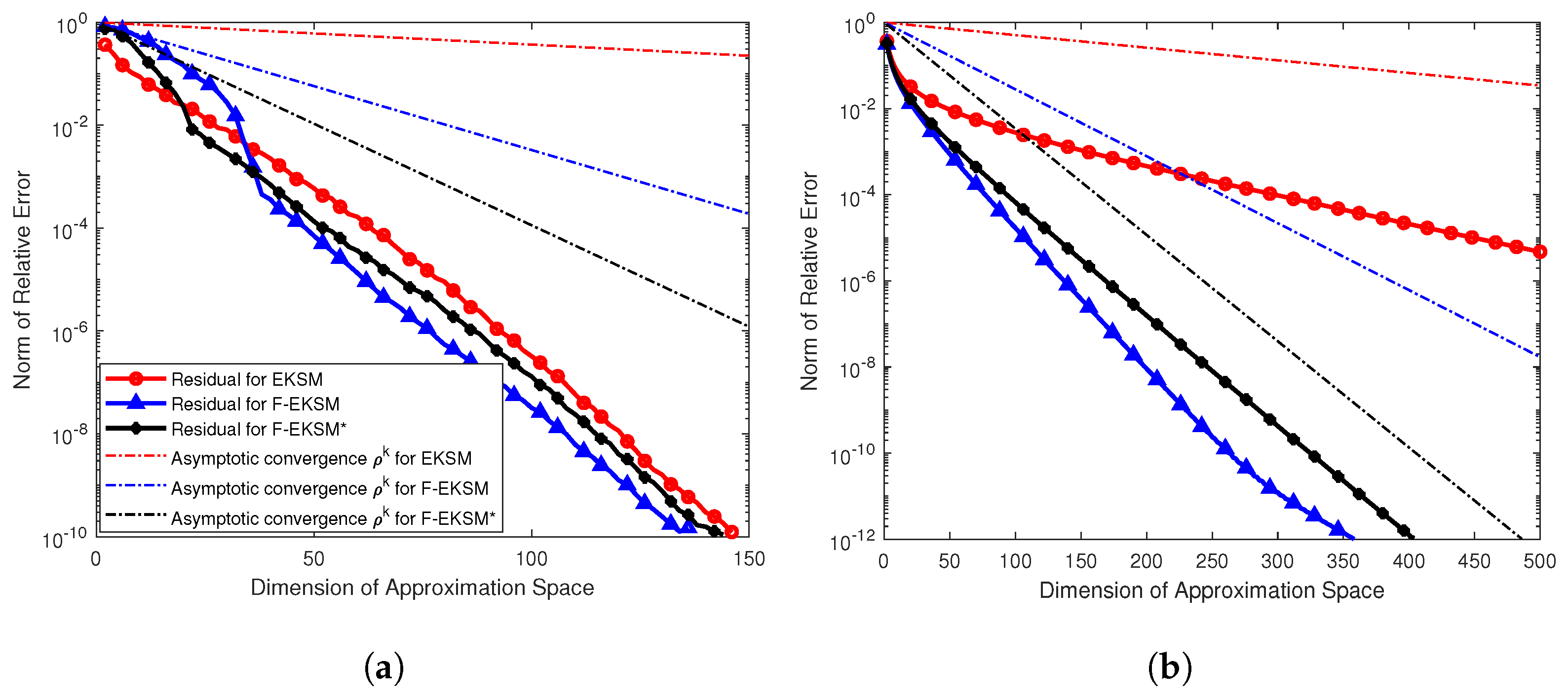
To check the asymptotic convergence factor for each method, it is necessary to know the exact vector $f\left(A\right)b$ for a given matrix A and vector b in order to calculate the norm of the residual at each step. For relatively large matrices it is only possible to directly evaluate the exact $f\left(A\right)b$ for diagonal matrices within a reasonable time. Because each SPD matrix is orthogonally similar to the diagonal matrix of its eigenvalues, our experiment results can be expected to reflect the behavior of EKSM, $\mathcal{F}$-EKSM, and $\mathcal{F}$-EKSM* applied to more general SPD matrices.

We constructed two diagonal matrices $A_1,A_2$. The diagonal entry $d_j$ for $A_1$ is $d_j=({\alpha }_1+{\beta }_1)/2+cos\left({\theta }_j\right)({\beta }_1-{\alpha }_1)/2$, $1\le j\le$ 10,000, where the ${\theta }_j$s are uniformly distributed on the interval $\left[0,2\pi \right]$ and ${\alpha }_1={10}^{-7}$, ${\beta }_1=1$. The diagonal entry $d_j$ for $A_2$ is $d_j={10}^{-8}{\rho }_2^{(j-1)}$, $1\le j\le$ 20,000, ${\rho }_2=1.001$. We approximated $f_i\left(A_i\right)b$ using EKSM, $\mathcal{F}$-EKSM, and $\mathcal{F}$-EKSM*, where b is a fixed vector with entries of standard normally distributed random numbers. The experimental results are shown in Figure 1.

Figure 1. Actual and asymptotic convergence of EKSM, $\mathcal{F}$-EKSM, and $\mathcal{F}$-EKSM* for SPD matrices: (a) $f_1\left(A_1\right)b$, $\kappa ={10}^8$ and (b) $f_2\left(A_2\right)b$, $\kappa =4.799\times {10}^8$.

From the figures for different Markov-type functions, it can be seen that all methods converge with factors no worse than their theoretical bounds, which verifies the validity of the results shown in Theorem 1. Moreover, $\mathcal{F}$-EKSM and $\mathcal{F}$-EKSM* always converge faster than EKSM for all the test functions and matrices. In particular, for approximating $f_2\left(A_2\right)b$, our $\mathcal{F}$-EKSM only takes about one quarter as many iterations to achieve a relative error less than ${10}^{-5}$ as compared to EKSM. Furthermore, the theoretical bounds are not always sharp for those methods.

For nonsymmetric matrices with elliptic numerical ranges, the theoretical convergence rate cannot be derived by an explicit formula; Table 1 shows the numerical results. To verify these results, we constructed a block diagonal matrix $A_3\in {\mathbb{R}}^{4901\times 4901}$ with $2\times 2$ diagonal blocks with eigenvalues that lie on the circle centered at $z=5000.5$ with radius $4999.5$. We then constructed another block diagonal matrix $A_4\in {\mathbb{R}}^{4901\times 4901}$ with eigenvalues that lie in the ellipse centered at $z=5000.5$, with a semi-major axis $4999.5$ and semi-minor axis $714.2$. The optimal pole for $\mathcal{F}$-EKSM can be computed using the strategy described in Section 4.2 ($s_3^{*}=-20.87$ and $s_4^{*}=-11.02$). Figure 2 shows the spectra of the matrices $A_i$, $A_i^{-1}$ and ${(I-A_i/s_i^{*})}^{-1}$ for $i=3,4$. Figure 3 shows the results for the nonsymmetric matrices. Table 1 shows the asymptotic convergence factors of EKSM and $\mathcal{F}$-EKSM for matrices $A_3$ and $A_4$, where $\beta ={10}^4$, $\eta =1$, ${\rho }_{\mathcal{F}EK}^{*}=0.65$, and ${\rho }_{EK}=0.82$ for $A_3$, while $\beta ={10}^4$, $\eta =0.75$, ${\rho }_{\mathcal{F}EK}^{*}=0.84$, and ${\rho }_{EK}=0.95$ for $A_4$.

Figure 2. Spectra of several matrices: (a) spectrum of $A_3$; (b) spectrum of $A_3^{-1}$; (c) spectrum of ${(I-A_3/s_3^{*})}^{-1}$; (d) spectrum of $A_4$; (e) spectrum of $A_4^{-1}$; (f) spectrum of ${(I-A_4/s_4^{*})}^{-1}$.

Figure 3. Performance and theoretical asymptotic convergence of EKSM and $\mathcal{F}$-EKSM for nonsymmetric matrices with elliptic spectra: (a) approximating $f_1\left(A_3\right)b$; (b) approximating $f_4\left(A_4\right)b$.

Similar to the results for SPD matrices, $\mathcal{F}$-EKSM converges faster than EKSM for the two artificial nonsymmetric problems. The upper bounds on the convergence factor in Table 1 match the actual convergence factor quite well.

6.2. Test for Practical SPD Matrices

Next, we tested EKSM, $\mathcal{F}$-EKSM, $\mathcal{F}$-EKSM*, and adaptive RKSM on several SPD matrices and compared their runtimes and the dimension of their approximation subspaces. Note that for general SPD matrices the largest and smallest eigenvalues are usually not known in advance. The Lanczos method or its restarted variants can be applied to estimate them, and this computation time should be taken into consideration for $\mathcal{F}$-EKSM and $\mathcal{F}$-EKSM*. The variant of EKSM in (5) is not considered in this section, as there is no convergence theory to compare with the actual performance and the convergence rate largely depends on the choice of l and m in (5).

For the SPD matrices, we used Cholesky decomposition with approximate minimum degree ordering to solve the linear systems involving A or $I-A/s$ for all four methods. The stopping criterion of all methods was to check whether the angle between the approximate solutions obtained at two successive steps fell below a certain tolerance. EKSM and $\mathcal{F}$-EKSM, and $\mathcal{F}$-EKSM* all apply the Lanczos three-term recurrence and perform local re-orthogonalization to enlarge the subspace, whereas adaptive RKSM applies a full orthogonalization process with global re-orthogonalization.

We tested four 2D discrete Laplacian matrices of orders ${128}^2$, ${256}^2$, ${512}^2$, and ${1024}^2$ based on standard five-point stencils on a square. For all problems, the vector b was a vector with entries of standard normally distributed random numbers, allowing the behavior of all four methods to be compared for matrices with different condition numbers.

Table 3 reports the runtimes and the dimensions of the rational Krylov subspaces that the four methods entail when applied to all test problems; in the table, EK, FEK, and ARK are abbreviation of EKSM, $\mathcal{F}$-EKSM, and adaptive RKSM, respectively. The stopping criterion was that the angle between the approximate solutions from two successive steps was less than $\tau ={10}^{-9}$. The single pole $s^{*}$ results for $\mathcal{F}$-EKSM are $-352.26,-569.84,-915.56$, and $-1464.6$, respectively, while for $\mathcal{F}$-EKSM* the $\widetilde{s^{*}}$ results are $-140.89,-227.29,-364.53$, and $-582.43$, respectively. The shortest CPU time appearing in each line listed in the table is marked in bold.

Table 3. Performance of EKSM, $\mathcal{F}$-EKSM, $\mathcal{F}$-EKSM*, and adaptive RKSM on SPD problems.

		Time (s)				Space Dimension
Function	Problem	EK	FEK	FEK*	ARK	EK	FEK	FEK*	ARK
$f_1$	Lap. A	$0.28$	$\mathbf{0}.\mathbf{19}$	$0.23$	$0.70$	52	42	46	22
	Lap. B	$1.10$	$\mathbf{0}.\mathbf{70}$	$0.88$	$3.70$	76	52	60	25
	Lap. C	$7.35$	$\mathbf{4}.\mathbf{49}$	$5.21$	$19.30$	102	66	76	28
	Lap. D	$43.36$	$\mathbf{24}.\mathbf{52}$	$27.82$	$100.96$	138	84	96	30
$f_2$	Lap. A	$\mathbf{0}.\mathbf{18}$	$0.20$	$\mathbf{0}.\mathbf{18}$	$0.94$	32	48	34	28
	Lap. B	$\mathbf{0}.\mathbf{48}$	$0.87$	$0.63$	$4.32$	30	60	40	32
	Lap. C	$\mathbf{2}.\mathbf{66}$	$5.55$	$3.62$	$27.72$	38	80	54	38
	Lap. D	$\mathbf{10}.\mathbf{44}$	$27.60$	$18.10$	$135.63$	36	96	64	39
$f_3$	Lap. A	$0.29$	$\mathbf{0}.\mathbf{22}$	$0.26$	$0.69$	52	42	46	22
	Lap. B	$1.17$	$\mathbf{0}.\mathbf{71}$	$0.88$	$3.26$	76	52	60	25
	Lap. C	$7.55$	$\mathbf{4}.\mathbf{49}$	$5.28$	$19.36$	102	66	76	28
	Lap. D	$43.15$	$\mathbf{23}.\mathbf{81}$	$27.61$	$101.28$	138	84	96	30
$f_4$	Lap. A	$0.21$	$\mathbf{0}.\mathbf{18}$	$0.20$	$0.71$	50	38	42	23
	Lap. B	$0.88$	$\mathbf{0}.\mathbf{60}$	$0.74$	$3.55$	66	46	54	27
	Lap. C	$6.29$	$\mathbf{3}.\mathbf{90}$	$4.63$	$20.71$	90	58	68	30
	Lap. D	$36.09$	$\mathbf{19}.\mathbf{76}$	$23.76$	$114.46$	120	72	84	33
$f_5$	Lap. A	$0.32$	$\mathbf{0}.\mathbf{17}$	$0.24$	$0.67$	48	36	42	21
	Lap. B	$1.04$	$\mathbf{0}.\mathbf{65}$	$0.77$	$3.20$	66	46	52	24
	Lap. C	$6.28$	$\mathbf{3}.\mathbf{81}$	$4.53$	$18.60$	88	56	66	27
	Lap. D	$35.06$	$\mathbf{19}.\mathbf{34}$	$23.90$	$97.79$	116	70	84	29

With only one exception, that of $f_2\left(z\right)=e^{-\sqrt{z}}$, it is apparent that $\mathcal{F}$-EKSM converges the fastest of the four methods in terms of wall clock time for all the test functions and matrices with different condition numbers. While $\mathcal{F}$-EKSM takes more steps than adaptive RKSM to converge, it requires fewer steps than EKSM. Furthermore, the advantage of $\mathcal{F}$-EKSM becomes more pronounced for matrices with a larger condition number. Notably, the advantage of $\mathcal{F}$-EKSM in terms of computation time is stronger than in terms of the spatial dimension, which is due to the orthogonalization cost being proportional to the square of the spatial dimension. $\mathcal{F}$-EKSM* takes slightly more steps than $\mathcal{F}$-EKSM to converge in these examples, and both methods have similar computation times.

The unusual behavior of all methods for $f_2\left(z\right)=e^{-\sqrt{z}}$ can be explained as follows. For these Laplacian matrices, the largest eigenvalues ${\lambda }_{max}$ range from $1.3\times {10}^5$ to $8.4\times {10}^6$. Because $f_2\left({\lambda }_{min}\right)\approx 0.0118$ and $f_2\left({\lambda }_{max}\right)\le f_2\left({10}^5\right)\approx 4.6\times {10}^{-138}$ (because $f_2$ decreases monotonically on $[0,\infty )$), the eigenvector components in vector b associated with relatively large eigenvalues would be eliminated in vector $f_2\left(A\right)b$ in double precision. In fact, because $\frac{f_2\left({10}^3\right)}{f_2\left({\lambda }_{min}\right)}\approx 1.6\times {10}^{-12}\approx \tau$, all eigenvalues of A greater than ${10}^3$ are essentially ‘invisible’ for $f_2$ under tolerance $\tau ={10}^{-12}$, and the effective condition number of all four Laplacian matrices is about $\frac{{10}^3}{{\lambda }_{min}}\approx 51$. As a result, it takes EKSM the same number of steps to converge for all these matrices; the shift for $\mathcal{F}$-EKSM and $\mathcal{F}$-EKSM* computed using ${\lambda }_{min}$ and ${\lambda }_{max}$ of these matrices is in fact not optimal for matrices with such a small effective condition number.

The pole $s^{*}$ in (17) for the SPD matrix is optimal, as we have proved that it has the smallest asymptotic convergence factor among all choices of the single pole. In order to numerically compare the behaviors for different setting of the single pole, we tested matrices Lap. B and Lap. C in Table 3 with $f_1$ and $f_3$, respectively. For each problem, we tested $\mathcal{F}$-EKSM by setting different single poles s to $s^{*}$, $2s^{*}$, $s^{*}/2$, $10s^{*}$, $s^{*}/10$ and setting $\widetilde{s^{*}}$ for $\mathcal{F}$-EKSM*. Figure 4 shows the experimental results. It can be seen that $\mathcal{F}$-EKSM has the fastest asymptotic convergence rate among all the 6 different values of single poles when setting the optimal single pole $s^{*}$, which confirms that $s^{*}$ is indeed optimal in our experiments.

Figure 4. Convergence of $\mathcal{F}$-EKSM for different setting of single poles: (a) $f_1$ on Lap. B and (b) $f_3$ on Lap. C.

6.3. Test for Practical Nonsymmetric Matrices

We consider 18 nonsymmetric real matrices, all of which have all eigenvalues on the right half of the complex plane. While these are all real sparse matrices, they all have complex eigenvalues with positive real parts. Half are in the form of $M^{-1}K$, where both M and K are sparse and $A=M^{-1}K$ is not formed explicitly. Table 4 reports several features for each matrix A: the matrix size is n, the smallest and largest eigenvalues in terms of absolute value are $\left|{\lambda }_{\mathrm{sm}}\right|$ and $\left|{\lambda }_{\mathrm{lm}}\right|$, respectively, the smallest and largest real parts of the eigenvalues are $\mathrm{Re}\left({\lambda }_{\mathrm{sr}}\right)$ and $\mathrm{Re}\left({\lambda }_{\mathrm{lr}}\right)$, respectively, and the largest imaginary part of the eigenvalues is $\mathrm{Im}\left({\lambda }_{\mathrm{li}}\right)$. Note that all these original matrices have spectra strictly in the left half of the complex plane; we simply switched their signs to make $f\left(A\right)$ well-defined for Markov-type functions.

Table 4. Selected features of the test problems.

Problem	Size n	$\left|{\mathit{\lambda }}_{\mathbf{sm}}\right|$	$\left|{\mathit{\lambda }}_{\mathbf{lm}}\right|$	$\mathbf{Re}\left({\mathit{\lambda }}_{\mathbf{sr}}\right)$	$\mathbf{Re}\left({\mathit{\lambda }}_{\mathbf{lr}}\right)$	$\mathbf{Im}\left({\mathit{\lambda }}_{\mathbf{li}}\right)$	$-{\mathit{s}}^{*}$	Tol
aerofoilA	16,388	$8.41\times {10}^{-2}$	$1.02\times {10}^3$	$1.04\times {10}^{-2}$	$1.01\times {10}^3$	$8.12\times {10}^2$	$1.185$	${10}^{-11}$
aerofoilB	23,560	$2.73\times {10}^{-1}$	$2.63\times {10}^2$	$2.73\times {10}^{-1}$	$1.43\times {10}^2$	$2.60\times {10}^2$	$2.447$	${10}^{-13}$
matRe500A	3595	$4.00\times {10}^{-1}$	$1.21\times {10}^2$	$-2.01\times {10}^{-1}$	$1.21\times {10}^2$	$1.12\times {10}^2$	$1.805$	${10}^{-12}$
matRe500B	9391	$3.00\times {10}^{-1}$	$5.22\times {10}^2$	$-4.04\times {10}^{-1}$	$5.22\times {10}^2$	$1.98\times {10}^2$	$3.331$	${10}^{-12}$
matRe500C	22,385	$2.78\times {10}^{-1}$	$1.56\times {10}^3$	$-4.49\times {10}^{-1}$	$1.56\times {10}^3$	$2.70\times {10}^2$	$4.666$	${10}^{-12}$
matRe500D	50,527	$2.84\times {10}^{-1}$	$5.11\times {10}^3$	$-3.28\times {10}^{-1}$	$5.11\times {10}^3$	$3.76\times {10}^2$	$7.163$	${10}^{-12}$
matRe500E	110,620	$2.62\times {10}^{-1}$	$1.38\times {10}^4$	$-3.07\times {10}^{-1}$	$1.38\times {10}^4$	$5.37\times {10}^2$	$9.548$	${10}^{-12}$
obstacle	37,168	$2.84\times {10}^{-1}$	$2.95\times {10}^5$	$2.91\times {10}^{-2}$	$2.95\times {10}^5$	$1.50\times {10}^2$	$6.273$	${10}^{-10}$
plate	37,507	$1.00\times {10}^{-2}$	$8.71\times {10}^4$	$7.35\times {10}^{-4}$	$8.71\times {10}^4$	$1.32\times {10}^2$	$2.021$	${10}^{-9}$
tolosa	4000	$1.18\times {10}^{+1}$	$4.84\times {10}^3$	$1.56\times {10}^{-1}$	$1.45\times {10}^3$	$4.62\times {10}^3$	$6.772$	${10}^{-7}$
raefsky3	21,200	$6.63\times {10}^{-6}$	$7.99\times {10}^5$	$6.63\times {10}^{-6}$	$7.99\times {10}^5$	$1.42\times {10}^0$	$0.033$	${10}^{-6}$
step	96,307	$5.87\times {10}^{-3}$	$2.18\times {10}^4$	$5.87\times {10}^{-3}$	$2.18\times {10}^4$	$6.61\times {10}^1$	$0.903$	${10}^{-9}$
cavity	37,507	$7.53\times {10}^{-3}$	$2.51\times {10}^7$	$4.99\times {10}^{-3}$	$2.51\times {10}^7$	$7.16\times {10}^2$	$11.25$	${10}^{-8}$
convdiffA	146,689	$2.37\times {10}^{+1}$	$5.69\times {10}^2$	unknown	$5.62\times {10}^2$	$3.73\times {10}^2$	$41.32$	${10}^{-13}$
convdiffB	146,689	$7.88\times {10}^{+1}$	$1.35\times {10}^3$	unknown	$3.98\times {10}^2$	$1.33\times {10}^3$	$317.2$	${10}^{-13}$
convdiffC	146,689	$2.14\times {10}^{+2}$	$3.84\times {10}^3$	unknown	$3.63\times {10}^2$	$3.83\times {10}^3$	$117.4$	${10}^{-13}$
gt01r	7980	$5.87\times {10}^{-1}$	$1.96\times {10}^4$	$1.33\times {10}^{-1}$	$2.84\times {10}^3$	$1.96\times {10}^4$	$18.09$	${10}^{-11}$
venkat	62,424	$5.50\times {10}^{-5}$	$1.08\times {10}^1$	$5.50\times {10}^{-5}$	$1.08\times {10}^1$	$2.21\times {10}^0$	$0.003$	${10}^{-11}$

For the single pole of $\mathcal{F}$-EKSM and the initial pole of the four-pole variant (4Ps) in Section 5, we used the optimal pole for the SPD case matrices (17) by setting $\alpha =min\left\{\left|{\lambda }_{\mathrm{lm}}\right|,\mathrm{Re}\left({\lambda }_{\mathrm{sr}}\right)\right\}$ and $\beta =max\left\{\left|{\lambda }_{\mathrm{lm}}\right|,\mathrm{Re}\left({\lambda }_{\mathrm{lr}}\right)\right\}$. The same setting of $\alpha$ and $\beta$ for building the Riemann mapping ${\varphi }_1\left(z\right)$ in (14) was applied to compute the optimal pole for $\mathcal{F}$-EKSM* in (20). In particular, because precise evaluation of $\alpha$ and $\beta$ is time-consuming, we approximated them using the ‘eigs’ function in MATLAB, which is based on the Krylov–Schur Algorithm; see, e.g., [55]. We set the residual tolerance to equal ${10}^{-3}$ for ‘eigs’, ensuring that all the test matrices could find the largest and smallest eigenvalues within a reasonable time. Higher accuracy in computing the eigenvalues is not required when determining the optimal pole, as the convergence performance for $\mathcal{F}$-EKSM does not change noticeably with tiny changes of the value of the pole. Note that the single pole we used for each problem is independent of the Markov-type function; see Table 4. For nonsymmetric matrices, we used LU factorizations to solve the linear systems involving coefficient matrices of A or $I-A/s$ for all methods. The stopping criterion was either when the angle between the approximate solutions was less than a tolerance for two successive steps, or when the dimension of the Krylov subspaces reached 1000. There have been a few discussions about restarting for approximating $f\left(A\right)b$, though only for polynomial approximation based on Arnoldi-like methods; see, e.g., [17,56]. In this paper, we only focus on the comparison of convergence rates for several different Krylov methods without restarting. Here, we need to choose a proper tolerance for each problem such that it is small enough to fully exhibit the rate of convergence for all methods while not being too small to satisfy. The last column of Table 4 reports the tolerances, which are fixed regardless of the different Markov-type functions.

In Table 5, Table 6, Table 7, Table 8 and Table 9, we report the runtime and dimension of the approximation spaces that the four methods entail for approximating $f_i\left(A\right)b$ to the specified tolerances. The runtime includes the time spent on the evaluation of optimal poles for $\mathcal{F}$-EKSM, $\mathcal{F}$-EKSM*, and the four-pole variant. The “−” symbol indicates failure to find a sufficiently accurate solution when the maximum dimension of approximation space (1000) was reached. The shortest CPU time appeared in each line of the listed tables is marked in bold. Figure 5 shows an example plot for each method, with the relative error $sin\angle (q_{k+1},q_k)$ (where $q_k$ is the approximation to $f\left(A\right)b$ at step k) plotted against the dimension of the approximation space for each function.

Table 5. Performance of five rational Krylov subspace methods for the function $f_1\left(z\right)=z^{-1/2}$.

	Time (s)					Space Dimension
Problem	EK	FEK	FEK*	ARK	4Ps	EK	FEK	FEK*	ARK	4Ps
aerofoilA	$29.59$	$10.43$	$13.22$	$23.36$	$\mathbf{5}.\mathbf{63}$	504	278	330	54	94
aerofoilB	$6.34$	$\mathbf{4}.\mathbf{70}$	$5.34$	$26.03$	$5.59$	206	138	156	44	75
matRe500A	$0.98$	$0.80$	$0.95$	$1.60$	$\mathbf{0}.\mathbf{77}$	140	100	120	41	67
matRe500B	$2.81$	$\mathbf{2}.\mathbf{22}$	$2.73$	$6.21$	$2.37$	170	116	142	45	80
matRe500C	$7.17$	$5.39$	$6.56$	$17.48$	$\mathbf{5}.\mathbf{21}$	214	146	172	46	88
matRe500D	$19.06$	$16.37$	$16.18$	$51.95$	$\mathbf{12}.\mathbf{80}$	264	200	200	50	92
matRe500E	$54.03$	$45.71$	$43.07$	$139.99$	$\mathbf{30}.\mathbf{97}$	324	248	236	53	92
obstacle	$28.04$	$14.58$	$19.74$	$36.10$	$\mathbf{10}.\mathbf{65}$	376	226	290	50	104
plate	$25.16$	$19.91$	$23.43$	$51.20$	$\mathbf{15}.\mathbf{61}$	316	198	240	35	85
tolosa	$1.44$	$1.14$	$1.47$	$\mathbf{0}.\mathbf{18}$	$0.59$	174	154	164	31	76
raefsky3	−	−	−	$15.79$	$\mathbf{6}.\mathbf{36}$	−	−	−	28	48
step	$67.41$	$45.12$	$52.46$	$110.92$	$\mathbf{36}.\mathbf{01}$	364	192	224	40	69
cavity	−	$173.99$	$59.17$	$39.21$	$\mathbf{19}.\mathbf{12}$	−	938	540	42	134
convdiffA	$\mathbf{16}.\mathbf{75}$	$32.12$	$19.06$	$36.87$	$20.05$	108	128	78	39	61
convdiffB	$19.47$	$23.25$	$14.80$	$33.62$	$\mathbf{14}.\mathbf{22}$	118	120	86	39	67
convdiffC	$17.70$	$21.86$	$14.18$	$34.58$	$\mathbf{13}.\mathbf{59}$	112	116	82	39	63
GT01R	$32.07$	$18.49$	$8.74$	$12.58$	$\mathbf{4}.\mathbf{64}$	600	472	328	63	151
venkat	$60.62$	$37.67$	$13.51$	$30.22$	$\mathbf{8}.\mathbf{72}$	528	400	210	40	69

Table 6. Performance of five rational Krylov subspace methods for the function $f_2\left(z\right)=e^{-\sqrt{z}}$.

	Time (s)					Space Dimension
Problem	EK	FEK	FEK*	ARK	4Ps	EK	FEK	FEK*	ARK	4Ps
aerofoilA	$36.69$	$8.55$	$15.60$	$22.82$	$\mathbf{5}.\mathbf{77}$	528	250	354	55	98
aerofoilB	$7.26$	$\mathbf{4}.\mathbf{41}$	$5.94$	$28.71$	$5.34$	218	126	168	50	71
matRe500A	$1.14$	$0.88$	$1.08$	$1.82$	$\mathbf{0}.\mathbf{75}$	150	110	130	45	68
matRe500B	$3.43$	$\mathbf{2}.\mathbf{37}$	$2.95$	$6.75$	$2.65$	184	126	150	49	88
matRe500C	$8.50$	$\mathbf{5}.\mathbf{57}$	$7.56$	$21.21$	$5.72$	228	150	192	57	100
matRe500D	$22.45$	$15.13$	$17.15$	$57.99$	$\mathbf{13}.\mathbf{44}$	290	186	210	56	100
matRe500E	$61.06$	$42.70$	$49.31$	$168.76$	$\mathbf{33}.\mathbf{15}$	350	234	264	63	104
obstacle	$31.66$	$15.23$	$22.72$	$40.76$	$\mathbf{9}.\mathbf{16}$	408	234	312	56	83
plate	$35.45$	$24.05$	$26.59$	$64.00$	$\mathbf{15}.\mathbf{42}$	388	244	268	44	81
tolosa	$2.41$	$2.08$	$2.22$	$\mathbf{0}.\mathbf{32}$	$6.92$	210	194	198	46	233
raefsky3	−	$42.25$	$110.27$	$17.21$	$\mathbf{8}.\mathbf{10}$	−	548	804	31	96
step	$89.53$	$46.87$	$61.80$	$119.95$	$\mathbf{36}.\mathbf{88}$	434	204	278	44	82
cavity	−	$164.15$	$56.39$	$46.52$	$\mathbf{16}.\mathbf{65}$	−	824	504	50	102
convdiffA	$21.92$	$31.98$	$20.91$	$42.67$	$\mathbf{20}.\mathbf{55}$	126	128	86	44	64
convdiffB	$23.26$	$25.79$	$15.45$	$43.14$	$\mathbf{14}.\mathbf{01}$	130	128	92	48	64
convdiffC	$22.93$	$23.13$	$15.55$	$41.18$	$\mathbf{13}.\mathbf{64}$	128	120	92	46	64
GT01R	$50.13$	$17.77$	$10.52$	$12.87$	$\mathbf{3}.\mathbf{24}$	650	440	352	68	115
venkat	$60.80$	$15.39$	$14.05$	$33.22$	$\mathbf{8}.\mathbf{58}$	516	228	214	43	67

Table 7. Performance of five rational Krylov subspace methods for the function $f_3\left(z\right)=\frac{tanh\sqrt{z}}{\sqrt{z}}$.

	Time (s)					Space Dimension
Problem	EK	FEK	FEK*	ARK	4Ps	EK	FEK	FEK*	ARK	4Ps
aerofoilA	$55.22$	$10.67$	$21.92$	$22.07$	$\mathbf{5}.\mathbf{14}$	496	236	340	54	76
aerofoilB	$8.53$	$\mathbf{4}.\mathbf{41}$	$6.37$	$27.94$	$5.70$	210	118	158	49	75
matRe500A	$1.54$	$1.09$	$1.49$	$1.70$	$\mathbf{0}.\mathbf{79}$	140	104	124	42	59
matRe500B	$3.91$	$\mathbf{2}.\mathbf{52}$	$3.28$	$6.53$	$2.68$	172	112	138	46	80
matRe500C	$8.77$	$\mathbf{5}.\mathbf{59}$	$7.52$	$17.73$	$5.75$	208	136	174	47	92
matRe500D	$24.04$	$13.09$	$17.81$	$55.73$	$\mathbf{12}.\mathbf{67}$	266	150	200	54	88
matRe500E	$60.38$	$33.71$	$45.53$	$143.02$	$\mathbf{30}.\mathbf{38}$	322	174	238	54	92
obstacle	$35.95$	$16.59$	$23.63$	$35.95$	$\mathbf{11}.\mathbf{04}$	376	226	290	50	104
plate	$39.00$	$25.73$	$32.25$	$61.05$	$\mathbf{17}.\mathbf{28}$	362	236	282	42	101
tolosa	$2.57$	$1.99$	$2.30$	$\mathbf{0}.\mathbf{19}$	$0.80$	174	154	164	31	76
raefsky3	−	$75.56$	$173.31$	$17.84$	$\mathbf{9}.\mathbf{05}$	−	556	732	31	100
step	$86.80$	$46.22$	$62.19$	$142.57$	$\mathbf{36}.\mathbf{27}$	382	192	268	51	77
cavity	−	$45.50$	$96.82$	$46.38$	$\mathbf{20}.\mathbf{37}$	−	376	548	50	138
convdiffA	$\mathbf{17}.\mathbf{06}$	$29.98$	$19.30$	$35.20$	$18.25$	108	120	78	37	51
convdiffB	$20.37$	$23.29$	$\mathbf{14}.\mathbf{13}$	$35.40$	$14.61$	118	120	86	39	67
convdiffC	$18.79$	$21.79$	$\mathbf{13}.\mathbf{39}$	$33.17$	$13.73$	112	114	82	38	63
GT01R	$83.07$	$7.72$	$15.42$	$12.26$	$\mathbf{5}.\mathbf{42}$	606	242	328	66	151
venkat	$\mathbf{2}.\mathbf{48}$	$5.13$	$5.08$	$39.07$	$8.27$	66	64	64	50	59

Table 8. Performance of five rational Krylov subspace methods for the function $f_4\left(z\right)=z^{1/4}$.

	Time (s)					Space Dimension
Problem	EK	FEK	FEK*	ARK	4Ps	EK	FEK	FEK*	ARK	4Ps
aerofoilA	$42.22$	$10.18$	$17.33$	$23.64$	$\mathbf{5}.\mathbf{65}$	514	254	344	58	94
aerofoilB	$7.24$	$\mathbf{4}.\mathbf{51}$	$5.65$	$28.03$	$6.04$	204	122	156	49	87
matRe500A	$1.12$	$0.88$	$1.08$	$1.81$	$\mathbf{0}.\mathbf{82}$	138	100	120	44	71
matRe500B	$3.14$	$\mathbf{2}.\mathbf{35}$	$2.88$	$6.98$	$2.42$	168	114	140	50	79
matRe500C	$7.63$	$\mathbf{5}.\mathbf{17}$	$6.72$	$20.17$	$5.27$	210	134	170	54	87
matRe500D	$19.84$	$14.03$	$16.77$	$58.09$	$\mathbf{12}.\mathbf{62}$	258	166	198	56	88
matRe500E	$53.91$	$38.53$	$43.11$	$167.40$	$\mathbf{29}.\mathbf{82}$	316	206	232	63	88
obstacle	$30.11$	$16.19$	$22.36$	$47.98$	$\mathbf{11}.\mathbf{67}$	376	234	294	65	116
plate	$39.41$	$26.07$	$32.72$	$82.89$	$\mathbf{18}.\mathbf{73}$	388	254	308	56	121
tolosa	$1.87$	$1.68$	$1.86$	$\mathbf{0}.\mathbf{15}$	$0.68$	164	150	158	30	68
raefsky3	−	$48.82$	$103.27$	$23.58$	$\mathbf{7}.\mathbf{60}$	−	526	726	42	86
step	$91.72$	$46.64$	$59.19$	$168.31$	$\mathbf{36}.\mathbf{99}$	434	204	266	62	86
cavity	−	$128.72$	$81.85$	$69.43$	$\mathbf{25}.\mathbf{41}$	−	712	576	75	190
convdiffA	$\mathbf{15}.\mathbf{64}$	$29.43$	$18.71$	$36.12$	$19.66$	104	118	76	38	59
convdiffB	$19.18$	$19.98$	$\mathbf{14}.\mathbf{31}$	$37.46$	$16.27$	116	110	86	42	75
convdiffC	$17.22$	$19.49$	$\mathbf{13}.\mathbf{40}$	$36.65$	$15.15$	110	106	82	41	71
GT01R	$51.81$	$16.50$	$11.90$	$13.62$	$\mathbf{5}.\mathbf{27}$	608	388	336	70	163
venkat	$82.40$	$25.55$	$17.10$	$37.61$	$\mathbf{8}.\mathbf{95}$	552	294	226	48	67

Table 9. Performance of five rational Krylov subspace methods for the function $f_5\left(z\right)=log\left(z\right)$.

	Time (s)					Space Dimension
Problem	EK	FEK	FEK*	ARK	4Ps	EK	FEK	FEK*	ARK	4Ps
aerofoilA	$40.81$	$10.75$	$18.15$	$23.09$	$\mathbf{5}.\mathbf{89}$	516	256	344	55	94
aerofoilB	$7.39$	$\mathbf{4}.\mathbf{53}$	$5.87$	$27.81$	$5.98$	206	124	156	49	83
matRe500A	$1.38$	$1.01$	$1.25$	$1.79$	$\mathbf{0}.\mathbf{86}$	140	102	122	44	64
matRe500B	$3.45$	$\mathbf{2}.\mathbf{45}$	$3.07$	$6.76$	$2.60$	168	114	140	48	80
matRe500C	$7.87$	$\mathbf{5}.\mathbf{26}$	$7.00$	$19.28$	$5.41$	210	134	170	52	88
matRe500D	$20.17$	$14.70$	$16.95$	$50.55$	$\mathbf{12}.\mathbf{73}$	260	174	198	49	88
matRe500E	$54.72$	$41.43$	$43.04$	$145.27$	$\mathbf{30}.\mathbf{49}$	318	222	232	54	92
obstacle	$30.77$	$16.28$	$22.89$	$40.04$	$\mathbf{11}.\mathbf{73}$	376	230	294	55	112
plate	$34.92$	$25.61$	$32.11$	$72.58$	$\mathbf{18}.\mathbf{98}$	362	250	302	49	117
tolosa	$2.63$	$1.94$	$2.15$	$\mathbf{0}.\mathbf{23}$	$0.92$	170	154	160	30	76
raefsky3	−	−	−	$17.76$	$\mathbf{8}.\mathbf{07}$	−	−	−	31	88
step	$90.39$	$46.88$	$59.46$	$137.08$	$\mathbf{37}.\mathbf{45}$	434	204	266	51	85
cavity	−	$157.56$	$80.11$	$56.39$	$\mathbf{24}.\mathbf{96}$	−	796	582	61	178
convdiffA	$\mathbf{15}.\mathbf{85}$	$29.75$	$18.80$	$35.57$	$19.58$	104	120	76	38	59
convdiffB	$18.64$	$20.67$	$\mathbf{13}.\mathbf{72}$	$35.90$	$15.65$	114	112	84	40	71
convdiffC	$17.59$	$19.75$	$\mathbf{13}.\mathbf{43}$	$33.00$	$14.42$	110	108	82	38	67
GT01R	$47.93$	$20.42$	$12.02$	$12.34$	$\mathbf{5}.\mathbf{83}$	612	426	336	63	163
venkat	$72.81$	$28.59$	$15.32$	$36.06$	$\mathbf{8}.\mathbf{78}$	542	324	218	47	68

Figure 5. Decay of $sin\angle (q_k,q_{k+1})$ as the approximation space dimension increases: (a) $f_1$ on aerofoilA; (b) $f_2$ on matRe500E; (c) $f_3$ on plate; (d) $f_4$ on step.

In the ninety total cases for eighteen problems and five functions shown in Table 5, Table 6, Table 7, Table 8 and Table 9, the four-pole variant is the fastest in runtime in sixty cases and $\mathcal{F}$-EKSM is the fastest in fourteen cases. Among all cases when the four-pole variant is not the fastest, it is no more than $10\%$ slower than the fastest in twelve cases and 10–$20\%$ slower in eight cases.

Overall, the four-pole variant is the best in terms of runtime, though there are several exceptions. The first is tolosa, which is the only problem on which adaptive RKSM ran the fastest for all functions. For this problem, the dimension of the matrix is relatively small; this makes it more efficient to perform a new linear solver at each step, as the LU cost is cheap. Moreover, for tolosa, $\mathrm{Im}\left({\lambda }_{\mathrm{li}}\right)$ is close to $\left|{\lambda }_{\mathrm{lm}}\right|$, meaning that the algorithms based on repeated poles converge slower; see Table 1. The second exception is venkat, where the four-pole variant is not the fastest for $f_3$. In fact, for $f_3$, EKSM, $\mathcal{F}$-EKSM, and $\mathcal{F}$-EKSM* converge within a much smaller dimension of the approximation space than for the other functions. A possible explanation is that in computer arithmetic it is difficult to accurately capture the relative change in function values for $f_3$ at small variables, and venkat has majority of eigenvalues that are small in terms of absolute value. For example, $\frac{f_3\left(6\times {10}^{-5}\right)-f_3\left(6\times {10}^{-5}\left(1+{10}^{-7}\right)\right)}{f_3\left(6\times {10}^{-5}\right)}=2.0\times {10}^{-11}$, which means that a relative change of ${10}^{-7}$ in the independent variable of $f_3$ near $6\times {10}^{-5}$ can lead to a relative change of $2.0\times {10}^{-11}$ in function value; thus, $f_3$ fails to observe such a difference in input above the given tolerance ${10}^{-10}$. The third exception is convdiffA, for which EKSM is fastest for four out of all five functions. In fact, EKSM takes fewer steps to converge than $\mathcal{F}$-EKSM, which can be seen at the bottom right of Figure 5. A possible reason for this is that $\left|{\lambda }_{\mathrm{lm}}\right|$ and $\mathrm{Re}\left({\lambda }_{\mathrm{sr}}\right)$ can only be evaluated approximately by several iterations of the Arnoldi method, and sometimes their values cannot be found accurately. The ‘optimal’ pole based on inaccurate $\alpha$ can sometimes be far away from the real optimal pole. Notable, for this exception $\mathcal{F}$-EKSM* takes fewer steps to converge than EKSM, though it requires more computation time. This is because EKSM uses infinite poles; for the matrix in the form of $M^{-1}K$, where M is an identity matrix, it is not necessary to apply a linear solver for infinite poles, only a simple matrix vector multiplication. For the other cases in which $\mathcal{F}$-EKSM or $\mathcal{F}$-EKSM* runs fastest, the four-pole variant usually runs only slightly slower, as in those cases it takes less time to enlarge the approximation space than to compute more LU factorizations for using more repeated poles.

It is important to underscore that the runtime needed for $\mathcal{F}$-EKSM with our optimal pole is less than that for $\mathcal{F}$-EKSM* with an optimal pole derived based on [26] for a majority of the nonsymmetric test matrices, which is similar to the minor advantage in runtime of our $\mathcal{F}$-EKSM shown in Table 3 for Laplacian matrices. In addition, the runtime of the four-pole variant suggests that if sparse LU factorization is efficient for the shifted matrices needed for RKSM, then using a small number of near optimal poles seems to be an effective way to achieve the lowest overall runtime.

In terms of the dimension of the approximation space, adaptive RKSM always need the smallest subspace to converge, with the four-pole variant in second place except for $f_2$ for tolosa. In most, cases EKSM needs the largest subspace to converge, while in others $\mathcal{F}$-EKSM needs the largest subspace. In the cases where $\mathcal{F}$-EKSM and the four-pole variant converge, the four-pole variant takes $7.8\%$ to $87.6\%$ fewer steps.

In summary, our experiments suggest that $\mathcal{F}$-EKSM, $\mathcal{F}$-EKSM*, and the four-pole variant are competitive in reducing the runtime of rational Krylov methods based on direct linear solvers for approximating $f\left(A\right)b$; on the other hand, if the goal is to save storage cost, adaptive RKSM is preferable.

7. Conclusions

In this paper, we have studied an algorithm called the flexible extended Krylov subspace method ($\mathcal{F}$-EKSM) for approximating $f\left(A\right)b$ for Markov-type functions. The central idea is to find an optimal pole to replace the zero pole in EKSM such that $\mathcal{F}$-EKSM needs only the same single LU factorization as EKSM while converging more rapidly.

In the main theoretical contribution of this work, Theorem 1, we prove that there exists a unique optimal pole for a symmetric positive-definite matrix that guarantees the fastest convergence of $\mathcal{F}$-EKSM, which always outperforms EKSM. The theorem provides a formula for both the optimal pole and an upper bound on the convergence factor. Numerical experiments show that $\mathcal{F}$-EKSM is more efficient than EKSM and that it is competitive in runtime compared with adaptive RKSM if the shifted linear systems needed for rational Krylov methods are solved using a direct linear solver.

$\mathcal{F}$-EKSM may lose its advantages for challenging nonsymmetric matrices because of possible failure to compute the optimal poles numerically and due to its relatively slow convergence rate for these problems. This performance can be improved by using four fixed poles chosen flexibly in the early stage of computation. Our numerical results show that the four-pole variant is the most efficient in terms of runtime for many problems.

References

- Higham, N.J. Functions of Matrices: Theory and Computation; Society for Industrial and Applied Mathematics (SIAM): Philadelphia, PA, USA, 2008; pp. xx+425. [Google Scholar]
- Schilders, W.H.A.; van der Vorst, H.A.; Rommes, J. (Eds.) Model Order Reduction: Theory, Research Aspects and Applications; Mathematics in Industry; Springer: Berlin/Heidelberg, Germany, 2008; Volume 13, pp. xii+471. [Google Scholar]
- Grimm, V.; Hochbruck, M. Rational approximation to trigonometric operators. BIT 2008, 48, 215–229. [Google Scholar] [CrossRef][Green Version]
- Burrage, K.; Hale, N.; Kay, D. An efficient implicit FEM scheme for fractional-in-space reaction-diffusion equations. SIAM J. Sci. Comput. 2012, 34, A2145–A2172. [Google Scholar] [CrossRef]
- Bloch, J.C.; Heybrock, S. A nested Krylov subspace method to compute the sign function of large complex matrices. Comput. Phys. Commun. 2011, 182, 878–889. [Google Scholar] [CrossRef][Green Version]
- Kressner, D.; Tobler, C. Krylov subspace methods for linear systems with tensor product structure. SIAM J. Matrix Anal. Appl. 2010, 31, 1688–1714. [Google Scholar] [CrossRef]
- Hochbruck, M.; Ostermann, A. Exponential Runge-Kutta methods for parabolic problems. Appl. Numer. Math. 2005, 53, 323–339. [Google Scholar] [CrossRef]
- Hochbruck, M.; Lubich, C. Exponential integrators for quantum-classical molecular dynamics. BIT 1999, 39, 620–645. [Google Scholar] [CrossRef]
- Bai, Z. Krylov subspace techniques for reduced-order modeling of large-scale dynamical systems. Appl. Numer. Math. 2002, 43, 9–44. [Google Scholar] [CrossRef]
- Freund, R.W. Krylov-subspace methods for reduced-order modeling in circuit simulation. J. Comput. Appl. Math. 2000, 123, 395–421. [Google Scholar] [CrossRef]
- Wang, S.; de Sturler, E.; Paulino, G.H. Large-scale topology optimization using preconditioned Krylov subspace methods with recycling. Internat. J. Numer. Methods Engrg. 2007, 69, 2441–2468. [Google Scholar] [CrossRef]
- Biros, G.; Ghattas, O. Parallel Lagrange-Newton-Krylov-Schur methods for PDE-constrained optimization. I. The Krylov-Schur solver. SIAM J. Sci. Comput. 2005, 27, 687–713. [Google Scholar] [CrossRef]
- Simoncini, V. Computational methods for linear matrix equations. SIAM Rev. 2016, 58, 377–441. [Google Scholar] [CrossRef]
- Druskin, V.; Knizhnerman, L. Extended Krylov subspaces: Approximation of the matrix square root and related functions. SIAM J. Matrix Anal. Appl. 1998, 19, 755–771. [Google Scholar] [CrossRef]
- Bergamaschi, L.; Caliari, M.; Martínez, A.; Vianello, M. Comparing Leja and Krylov approximations of large scale matrix exponentials. In Proceedings of the Computational Science–ICCS 2006, Reading, UK, 28–31 May 2006; Springer: Berlin/Heidelberg, Germany, 2006; pp. 685–692. [Google Scholar]
- Knizhnerman, L.; Simoncini, V. Convergence analysis of the extended Krylov subspace method for the Lyapunov equation. Numer. Math. 2011, 118, 567–586. [Google Scholar] [CrossRef][Green Version]
- Eiermann, M.; Ernst, O.G. A restarted Krylov subspace method for the evaluation of matrix functions. SIAM J. Numer. Anal. 2006, 44, 2481–2504. [Google Scholar] [CrossRef]
- Frommer, A.; Simoncini, V. Stopping criteria for rational matrix functions of Hermitian and symmetric matrices. SIAM J. Sci. Comput. 2008, 30, 1387–1412. [Google Scholar] [CrossRef]
- Popolizio, M.; Simoncini, V. Acceleration techniques for approximating the matrix exponential operator. SIAM J. Matrix Anal. Appl. 2008, 30, 657–683. [Google Scholar] [CrossRef][Green Version]
- Bai, Z.Z.; Miao, C.Q. Computing eigenpairs of Hermitian matrices in perfect Krylov subspaces. Numer. Algorithms 2019, 82, 1251–1277. [Google Scholar] [CrossRef]
- Knizhnerman, L.; Simoncini, V. A new investigation of the extended Krylov subspace method for matrix function evaluations. Numer. Linear Algebra Appl. 2010, 17, 615–638. [Google Scholar] [CrossRef]
- Simoncini, V. A new iterative method for solving large-scale Lyapunov matrix equations. SIAM J. Sci. Comput. 2007, 29, 1268–1288. [Google Scholar] [CrossRef]
- Güttel, S.; Knizhnerman, L. A black-box rational Arnoldi variant for Cauchy-Stieltjes matrix functions. BIT 2013, 53, 595–616. [Google Scholar] [CrossRef]
- Druskin, V.; Simoncini, V. Adaptive rational Krylov subspaces for large-scale dynamical systems. Syst. Control Lett. 2011, 60, 546–560. [Google Scholar] [CrossRef]
- Benzi, M.; Simoncini, V. Decay bounds for functions of Hermitian matrices with banded or Kronecker structure. SIAM J. Matrix Anal. Appl. 2015, 36, 1263–1282. [Google Scholar] [CrossRef]
- Beckermann, B.; Reichel, L. Error estimates and evaluation of matrix functions via the Faber transform. SIAM J. Numer. Anal. 2009, 47, 3849–3883. [Google Scholar] [CrossRef]
- Xu, S.; Xue, F. Inexact rational Krylov subspace methods for approximating the action of functions of matrices. Electron. Trans. Numer. Anal. 2023, 58, 538–567. [Google Scholar] [CrossRef]
- Beckermann, B.; Güttel, S. Superlinear convergence of the rational Arnoldi method for the approximation of matrix functions. Numer. Math. 2012, 121, 205–236. [Google Scholar] [CrossRef]
- Hochbruck, M.; Lubich, C. On Krylov subspace approximations to the matrix exponential operator. SIAM J. Numer. Anal. 1997, 34, 1911–1925. [Google Scholar] [CrossRef]
- Druskin, V.; Knizhnerman, L. Krylov subspace approximation of eigenpairs and matrix functions in exact and computer arithmetic. Numer. Linear Algebra Appl. 1995, 2, 205–217. [Google Scholar] [CrossRef]
- Druskin, V.; Knizhnerman, L.; Zaslavsky, M. Solution of large scale evolutionary problems using rational Krylov subspaces with optimized shifts. SIAM J. Sci. Comput. 2009, 31, 3760–3780. [Google Scholar] [CrossRef]
- Druskin, V.; Knizhnerman, L.; Simoncini, V. Analysis of the rational Krylov subspace and ADI methods for solving the Lyapunov equation. SIAM J. Numer. Anal. 2011, 49, 1875–1898. [Google Scholar] [CrossRef]
- Berljafa, M.; Güttel, S. Generalized rational Krylov decompositions with an application to rational approximation. SIAM J. Matrix Anal. Appl. 2015, 36, 894–916. [Google Scholar] [CrossRef]
- Jagels, C.; Reichel, L. Recursion relations for the extended Krylov subspace method. Linear Algebra Appl. 2011, 434, 1716–1732. [Google Scholar] [CrossRef]
- Jagels, C.; Reichel, L. The extended Krylov subspace method and orthogonal Laurent polynomials. Linear Algebra Appl. 2009, 431, 441–458. [Google Scholar] [CrossRef]
- Ruhe, A. Rational Krylov sequence methods for eigenvalue computation. Linear Algebra Appl. 1984, 58, 391–405. [Google Scholar] [CrossRef]
- Ruhe, A. Rational Krylov algorithms for nonsymmetric eigenvalue problems. In Recent Advances in Iterative Methods; The IMA Volumes in Mathematics and Its Applications; Springer: New York, NY, USA, 1994; Volume 60, pp. 149–164. [Google Scholar]
- Güttel, S. Rational Krylov approximation of matrix functions: Numerical methods and optimal pole selection. GAMM-Mitt. 2013, 36, 8–31. [Google Scholar] [CrossRef]
- Bagby, T. The modulus of a plane condenser. J. Math. Mech. 1967, 17, 315–329. [Google Scholar] [CrossRef]
- Gončar, A.A. The problems of E. I. Zolotarev which are connected with rational functions. Mat. Sb. 1969, 78, 640–654. [Google Scholar]
- Caliari, M.; Vianello, M.; Bergamaschi, L. Interpolating discrete advection-diffusion propagators at Leja sequences. J. Comput. Appl. Math. 2004, 172, 79–99. [Google Scholar] [CrossRef]
- Caliari, M.; Vianello, M.; Bergamaschi, L. The LEM exponential integrator for advection-diffusion-reaction equations. J. Comput. Appl. Math. 2007, 210, 56–63. [Google Scholar] [CrossRef]
- Druskin, V.; Lieberman, C.; Zaslavsky, M. On adaptive choice of shifts in rational Krylov subspace reduction of evolutionary problems. SIAM J. Sci. Comput. 2010, 32, 2485–2496. [Google Scholar] [CrossRef]
- Ruhe, A. Rational Krylov: A practical algorithm for large sparse nonsymmetric matrix pencils. SIAM J. Sci. Comput. 1998, 19, 1535–1551. [Google Scholar] [CrossRef]
- Botchev, M.A.; Grimm, V.; Hochbruck, M. Residual, restarting, and Richardson iteration for the matrix exponential. SIAM J. Sci. Comput. 2013, 35, A1376–A1397. [Google Scholar] [CrossRef]
- Saad, Y. Analysis of some Krylov subspace approximations to the matrix exponential operator. SIAM J. Numer. Anal. 1992, 29, 209–228. [Google Scholar] [CrossRef]
- van den Eshof, J.; Hochbruck, M. Preconditioning Lanczos approximations to the matrix exponential. SIAM J. Sci. Comput. 2006, 27, 1438–1457. [Google Scholar] [CrossRef]
- Björck, A.; Golub, G.H. Numerical methods for computing angles between linear subspaces. Math. Comp. 1973, 27, 579–594. [Google Scholar] [CrossRef]
- De Sturler, E. Truncation strategies for optimal Krylov subspace methods. SIAM J. Numer. Anal. 1999, 36, 864–889. [Google Scholar] [CrossRef]
- Elman, H.C.; Su, T. Low-rank solution methods for stochastic eigenvalue problems. SIAM J. Sci. Comput. 2019, 41, A2657–A2680. [Google Scholar] [CrossRef]
- Bak, J.; Newman, D.J. Complex Analysis, 3rd ed.; Undergraduate Texts in Mathematics; Springer: New York, NY, USA, 2010; pp. xii+328. [Google Scholar]
- Suetin, P.K. Series of Faber Polynomials; Analytical Methods and Special Functions; Gordon and Breach Science Publishers: Amsterdam, The Netherlands, 1998; Volume 1, pp. xx+301. [Google Scholar]
- Crouzeix, M. Numerical range and functional calculus in Hilbert space. J. Funct. Anal. 2007, 244, 668–690. [Google Scholar] [CrossRef]
- Driscoll, T.A. Algorithm 843: Improvements to the Schwarz-Christoffel toolbox for MATLAB. ACM Trans. Math. Softw. 2005, 31, 239–251. [Google Scholar] [CrossRef]
- Stewart, G.W. A Krylov-Schur algorithm for large eigenproblems. SIAM J. Matrix Anal. Appl. 2001, 23, 601–614. [Google Scholar] [CrossRef]
- Frommer, A.; Güttel, S.; Schweitzer, M. Convergence of restarted Krylov subspace methods for Stieltjes functions of matrices. SIAM J. Matrix Anal. Appl. 2014, 35, 1602–1624. [Google Scholar] [CrossRef]
- Curtiss, J.H. Faber polynomials and the Faber series. Am. Math. Mon. 1971, 78, 577–596. [Google Scholar] [CrossRef]
- Duren, P.L. Univalent Functions; Fundamental Principles of Mathematical Sciences; Springer: New York, NY, USA, 1983; Volume 259, pp. xiv+382. [Google Scholar]
- Bronshtein, I.N.; Semendyayev, K.A.; Musiol, G.; Mühlig, H. Handbook of Mathematics, 6th ed.; Springer: Berlin/Heidelberg, Germany, 2015; pp. xliv+1207. [Google Scholar]
Disclaimer/Publisher’s Note: The statements, opinions and data contained in all publications are solely those of the individual author(s) and contributor(s) and not of MDPI and/or the editor(s). MDPI and/or the editor(s) disclaim responsibility for any injury to people or property resulting from any ideas, methods, instructions or products referred to in the content. |
© 2023 by the authors. Licensee MDPI, Basel, Switzerland. This article is an open access article distributed under the terms and conditions of the Creative Commons Attribution (CC BY) license (https://creativecommons.org/licenses/by/4.0/).