Extinctions in a Metapopulation with Nonlinear Dispersal Coupling

Abstract

Major threats to biodiversity are climate change, habitat fragmentation (in particular, habitat loss), pollution, invasive species, over-exploitation, and epidemics. Over the last decades habitat fragmentation has been given special attention. Many factors are causing biological systems to extinct; therefore, many issues remain poorly understood. In particular, we would like to know more about the effect of the strength of inter-site coupling (e.g., it can represent the speed with which species migrate) on species extinction or persistence in a fragmented habitat consisting of sites with randomly varying properties. To address this problem we use theoretical methods from mathematical analysis, functional analysis, and numerical methods to study a conceptual single-species spatially-discrete system. We state some simple necessary conditions for persistence, prove that this dynamical system is monotone and we prove convergence to a steady-state. For a multi-patch system, we show that the increase of inter-site coupling leads to the formation of clusters—groups of populations whose sizes tend to align as coupling increases. We also introduce a simple one-parameter sufficient condition for a metapopulation to persist.

1. Introduction

In recent decades, significant attention has been directed towards the factors and processes that lead to the survival or extinction of natural populations [1]. This focus has been spurred by ongoing global environmental changes, including the impact of global warming on populations and communities [2]. One specific consequence of global warming is the alteration of species ranges and the fragmentation of habitats. Additionally, habitat fragmentation can occur due to human activities such as forest logging and the construction of new roads. Both habitat fragmentation and general habitat loss have a noticeably detrimental impact on corresponding populations, often leading to species extinctions [3,4]. In fact, habitat fragmentation is widely recognized as the most significant threat to biodiversity on a global scale [5,6].

That is why it is importaint to understand population dynamics in a complex or fragmented habitat and there is indeed a large number empirical and theoretical studies addressing this issue [7,8,9,10,11,12,13,14,15,16]. The most widely used models of population dynamics in a fragmented habitat are metapopulation models [4,17,18,19,20,21,22]. In this framework, a fragmented habitat is viewed as a collection of separate sites, with subpopulations of a species residing in these sites. The subpopulations can be connected either through dispersal between sites or by a shared external factor with spatial correlations, such as weather fluctuations [23,24]. Metapopulation models can either be spatially implicit, where the state of the metapopulation is described by a single global variable, for example the fraction of occupied sites [4,17,18,19], or spatially explicit, where each site is characterized by its own ’local’ variables, such as the size of a specific subpopulation [10,16,25], the propability of a patch being inhabited [26] etc. The former case sometimes can show results similar to lattice models [27,28] and network models [29,30], particularly when the relative locations of sites are explicitly considered.

Numerous studies have investigated the persistence or extinction of metapopulations in relation to habitat geometry [26,31,32], as well as environmental and demographic stochasticity [33,34]. However, there is a noticeable scarcity of research that specifically explores the impact of coupling strength between different sites on persistence or extinction, even though it may be implicitly accounted for through habitat geometry, where coupling strength generally diminishes with greater inter-site distance. Nevertheless, understanding the impact of coupling strength is critical, especially in light of evidence suggesting that inter-site coupling might be altered due to climate change [35,36].

It should be noted that the possibility of extinction depends on the type of density-dependence observed in local population growth. In deterministic models, in a closed system (i.e., without outward migration), populations with logistic growth cannot go extinct because the extinction state is unstable [37,38,39]. However, natural populations rarely conform to logistic growth patterns. Instead, growth rates often exhibit the Allee effect [40,41,42,43], which can be caused by many factors that are often present in real-life situations [44]. The presence of a strong Allee effect significantly alters population dynamics [40,42,43,45,46,47,48]. Notably, the extinction state becomes stable, thus allowing for the possibility of extinction within a closed population.

For a two-site system studied previously [49], it was demonstrated that, subject to certain limitations, an increase in coupling strength can potentially trigger a population outbreak, where the system transitions from a low-density steady state to a high-density one. Mathematically, this transition corresponds to a saddle-node bifurcation, in which the low-density steady state vanishes as a consequence of increased coupling. Although with the model proposed below we focus on extinction rather than outbreaks, It will be shown that the extinction may follow a sufficiently large increase in the coupling strength due to essentially the same mechanism as in [49].

This paper complements the research done in [50] with linear coupling. Here we consider two types of coupling: linear and quadratic. This work differs from the work done in [50] in the sence that we use analytic methods from mathematical analysis, nonlinear functional analysis, monotone dynamical systems theory etc. The methods are used to prove some sufficient conditions for metapopulation persistence. We also show that the solutions are bounded and analytic and we study the asymptotic behavior for some initial conditions. In the end we present a one parameter criterion for a system to persist and estimate the parameter.

2. Materials and Methods

The existence of a non-zero steady-state point for the case with logistic growth will be proved analytically.

For the Allee effect we simulate both types of coupling using the RK45 method, which is programmed in Python using scipy.integrate.solve_ivp. This method with standard settings is perfect for the model with quadratic coupling; for linear coupling we will change the settings, see this section below. The Euler method is not very efficient here because of its slow convergence to the solution. Also the use of higher order methods can be motivated by analyticity of solutions. We do not consider Runge-Kutta methods of higher order because it is not necessary for our tasks. The RK45 method has global error on the order of $O\left(h^5\right)$ [51].

We let $u_i\left(0\right)=\max k_j$ and change q with a step size of $0.5$ from $0.5$ to 20. It was checked in simulations that $t=200$ was sufficiently large to ensure the system’s convergence to its steady-state distribution. For linear case we had to set the value of related tolerance to an error $rtol={10}^{-6}$ instead of default $rtol={10}^{-3}$ to ensure the convergence for large q.

In the section “Two-Patch System” we assume that the solution to the Cauchy problem exists and is unique and continuously differentiable for $t\ge 0$, it will be proved in the section “Multi-Patch System”, which is written more formally and states all necessary proofs. The section “Two-Patch System” helps become better acquainted with the model in a simpler case.

3. Two-Patch System

In this section we consider the systems with a linear and quadratic coupling. The linear coupling between two populations u and v is written as $q(u-v)$ for some coefficient q. The quadratic coupling between two populations u and v is written as $q(u^2-v^2)$ for some coefficient q.

The quadratic coupling is also called density-dependent dispersal. It is due to the fact that $u^2-v^2=(u+v)(u-v)$. So the strength of the coupling depends on the total population $u+v$.

Here we begin with a quadratic coupling as a continuation of the paper [50] with linear model. Then we list some additional properties for a linear coupling which can be analogously proven.

The dynamics of the two-patch system with a quadratic coupling is described by the following equations:

$$\frac{d{u}_1}{dt}=f_1\left(u_1\right)+q(u_2^2-u_1^2),\frac{d{u}_2}{dt}=f_2\left(u_2\right)+q(u_1^2-u_2^2),$$

(1)

where $f_1, f_2$ are polynomials of the same form such that $f_1\left(0\right)=f_2\left(0\right)=f_1\left(k_1\right)=f_2\left(k_2\right)=0$ for some positive real numbers $k_1, k_2$. Here we are considering polynomials of the forms $f_i\left(u_i\right)={\alpha }_i{u}_i(1-\frac{u_i}{k_i})$ (logistic growth) and $f_i\left(u_i\right)={\alpha }_i{u}_i(u_i-{\beta }_i)(1-\frac{u_i}{k_i})$ (logistic growth with an Allee effect) with positive coefficients, where ${\beta }_i<k_i$.

The properties of the system (1) are determined by its steady states; in particular, a long-term persistence of the two subpopulations is only possible if there exists a stable ‘coexistence’ steady state, i.e., a positive solution of the following system:

$$f_1\left(u_1\right)+q(u_2^2-u_1^2)=0,f_2\left(u_2\right)+q(u_1^2-u_2^2)=0.$$

(2)

From (2) we readly get:

$$f_1\left(u_1\right)+f_2\left(u_2\right)=0.$$

(3)

If $q\ne 0$, the system (2) can be rewritten as

$$u_2^2=u_1^2-\frac{1}{q}{f}_1\left(u_1\right),u_1^2=u_2^2-\frac{1}{q}{f}_2\left(u_2\right)$$

(4)

When $q\to \infty$, we get $u_1=u_2$.

Let $u_1\left(0\right)=u_{01},u_2\left(0\right)=u_{02}$. By ${\widehat{u}}_1,{\widehat{u}}_2$ further we will denote the steady state values for these initial conditions if they exist ( in a sence that $u_1\left(t\right)\to {\widehat{u}}_1,u_2\left(t\right)\to {\widehat{u}}_2$, when $t\to \infty$).

If there are steady state values, then $f_1\left({\widehat{u}}_1\right)+f_2\left({\widehat{u}}_2\right)=0$. So the Equation (3) is a necessary condition for a point $({\widehat{u}}_1,{\widehat{u}}_2)$ to be a steady state point.

We also define $\overline{u}=\frac{u_1+u_2}{2},{\overline{u}}_0=\overline{u}\left(0\right),\frac{d\overline{u}}{dt}=\frac{f_1\left(u_1\right)+f_2\left(u_2\right)}{2},Z\left(f\right)=\left\{u\right|f\left(u\right)=0\}$.

The case $q=0$ is not very interesting because the system (2) is simplified to $f\left(u_1\right)=0,$$f\left(u_2\right)=0$, hence, a point $({\widehat{u}}_1,{\widehat{u}}_2)$ is a steady state point iff $({\widehat{u}}_1,{\widehat{u}}_2)\in Z\left(f_1\right)\times Z\left(f_2\right)=\left\{(u_1,u_2)\right|f\left(u_1\right)=0,f\left(u_2\right)=0\}$.

There is another trivial case which is covered by Lemma 1.

Lemma 1.

Let $Z\left(f\right)=\left\{u\right|f\left(u\right)=0\}$. Then for any $\widehat{u}\in Z\left(f_1\right)\bigcap Z\left(f_2\right)$ we have a steady state point $(\widehat{u},\widehat{u})$.

Proof. 

We fix any $\widehat{u}\in Z\left(f_1\right)\bigcap Z\left(f_2\right)$. Let $u_{01}=\widehat{u},u_{02}=\widehat{u}$. Then $\frac{d{u}_1}{dt}\left(0\right)=\frac{d{u}_2}{dt}\left(0\right)=0$, hence, the point $(\widehat{u},\widehat{u})$ is a steady state point. □

Now we consider more specific models: logistic growth and logistic growth with an Allee effect. For the logistic growth the case $k_1=k_2$ is trivial, for other two cases it is enough to consider an example 1 below because another one becomes the example 1, if we change indexes.

Example 1.

$f_i\left(u_i\right)={\alpha }_i{u}_i(1-\frac{u_i}{k_i}),i=1,2,k_1>k_2$; $u_1\left(0\right)=k_2,u_2\left(0\right)=k_2$, $q\ne 0$. Then there is a non-zero steady state point.

Proof. 

We know that $\frac{d{u}_1}{dt}{|}_{u_1=u_2\ne 0}>0$ for $u_1=u_2<k_1$, hence, for all $t>0$ we have $u_1\left(t\right)>u_2\left(t\right)$. We note that $\frac{d\overline{u}}{dt}>0$ when $u_1\in [0;k_1],u_2\in [0;k_2]$. This means that the population cannot extinct because $\overline{u}\left(t\right)>k_2$ for all $t>0$, in other words, we got that for all $t>0$ $u_1\left(t\right)>u_2\left(t\right)>k_2$.

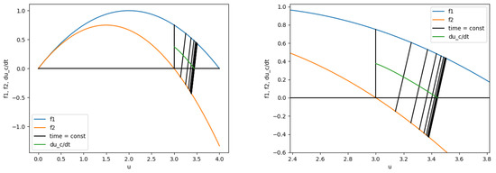
Let us now consider the behavior as $t\to \infty$ (Figure 1). We know that $\frac{d{u}_1}{dt}\left(0\right)>0$, the function $\frac{d{u}_1}{dt}$ is continuous, hence, it is positive in some neighborhood. It is also clear that for $i=1$ there exists $t_i>0$ ($t_i$ may be infinity) such that $\frac{d{u}_1}{dt}\left(t_i\right)=0$, otherwise there would be some constant $C_i>0$ such that $\frac{d{u}_1}{dt}>C_i$ that would lead to $u_1\to \infty$—it is a contradiction. So we have $\frac{d{u}_1}{dt}\left(t_i\right)=0$, and two cases: $t_i=\infty$, and $t_i\ne \infty$. If we have more than one point $t_i$ we number the set $T=\{t_i\in \mathbb{R}\bigcup \{\infty \}|\frac{d{u}_1}{dt}\left(t_i\right)=0\}$ in such way that for any integer i between 2 and $card\left(T\right)$ we will have $t_{i-1}<t_i$ (the set T is no more than countable because $\frac{d{u}_2}{dt}>0$).

Figure 1. The functions $u_1$, $u_2$ are monotonically increasing, the function $\frac{d\overline{u}}{dt}$ is monotonically decreasing and has a limit 0, that leads to an existence of a non-zero steady-state point. The first coordinate of the ends of the lines is the value of $u_1$ and $u_2$ at the particular time:time = const. The second coordinate of the centres of the lines is $\frac{d\overline{u}}{dt}$.

Let us first assume that $t_i\ne \infty$. $\frac{d{u}_2}{dt}>0$ while $\frac{d{u}_1}{dt}>0$, nontrivial solution of an autonomous system cannot approach a fixed point in finite time, hence, we have

$$\frac{d{u}_1}{dt}\left(t_i\right)=0,\frac{d{u}_2}{dt}\left(t_i\right)>0,$$

hence, for some ${\epsilon }_i>0$ for all $\epsilon \in (0;{\epsilon }_i]$ we have $\frac{d{u}_1}{dt}(t_i+\epsilon )>0,\frac{d{u}_2}{dt}(t_i+\epsilon )>0$. Repeating these actions again, if the function $\frac{d{u}_1}{dt}$ has infinite number of $t_i\ne \infty$ such that $\frac{d{u}_1}{dt}\left(t_i\right)=0$ and $\frac{d{u}_1}{dt}>0$ in some deleted neighborhood, we get that for any $i\in \mathbb{N}\setminus \left\{1\right\}{t}_{i-1}<t_i$ and

$$\frac{d{u}_1}{dt}\left(t_i\right)=0,\frac{d{u}_2}{dt}\left(t_i\right)>0.$$

It means that $\frac{d\overline{u}}{dt}\left(t\right)>0$ for all $t\in [0;\infty )$. The derivative $\frac{d\overline{u}}{dt}\left(t\right)$ must approach zero, otherwise there would be a constant $C>0$ such that $\frac{d\overline{u}}{dt}\left(t\right)>C$ for all $t\in [0;\infty ]$, leading to $u_1\to \infty (\infty \leftarrow \overline{u}<u_1)$, which contradicts with $u_1\le k_1$. Therefore, $\frac{d\overline{u}}{dt}(\infty )=\frac{d{u}_1}{dt}(\infty )=\frac{d{u}_2}{dt}(\infty )=0$ because all the derivatives were non-negative. It means that there is a non-zero steady-state point $({\overline{u}}_1,{\overline{u}}_2)$. Moreover, we also prooved that $\infty \in T$, and that $\frac{d{u}_2}{dt}>0$ while $\frac{d{u}_1}{dt}\ge 0$.

We are left to prove that there is a non-zero steady-state point $({\widehat{u}}_1,{\widehat{u}}_2)$ in case of finite number of zeros of the derivative $\frac{d{u}_1}{dt}$. If we let $t_0=0$ there is an index i such that $t_{i-1}<t_i=\infty$, ${\epsilon }_i=\infty$, for all $\epsilon \in (0;\infty )$ we have $\frac{d{u}_1}{dt}(t_{i-1}+\epsilon )>0,\frac{d{u}_2}{dt}(t_{i-1}+\epsilon )>0$. It means again that $\frac{d\overline{u}}{dt}\left(t\right)>0$ for all $t\in [0;\infty )$, hence, $\frac{d\overline{u}}{dt}(\infty )=\frac{d{u}_1}{dt}(\infty )=\frac{d{u}_2}{dt}(\infty )=0$, and there is a non-zero steady-state point $({\widehat{u}}_1,{\widehat{u}}_2)$. □

All stated above gives us a proof of a following theorem:

Theorem 1.

The system (1) with logistic growth functions has a non-zero steady state point.

Remark. 

Another proof of Theorem 1 is given in the Section 4.1 (Theorem 6).

Example 2.

$f_i\left(u_i\right)={\alpha }_i{u}_i(u_i-{\beta }_i)(1-\frac{u_i}{k_i}),i=1,2,k_1>k_2,{\beta }_1<k_2$; $u_1\left(0\right)=k_2,u_2\left(0\right)=k_2$. There is a non-zero steady state point—the proof is identical to the proof in the Example 1.

Further we will consider the system with $f_i\left(u_i\right)={\alpha }_i{u}_i(u_i-{\beta }_i)(1-\frac{u_i}{k_i}),i=1,2,k_1>k_2, {\beta }_1>k_2$.

Firstly, we note that if $q\le \underset{u_2\in ({\beta }_2;k_2)}{\max }\frac{f_2\left(u_2\right)}{u_2^2}$, then there is a steady state point $({\overline{u}}_1;{\overline{u}}_2),{\overline{u}}_1<{\overline{u}}_2\in ({\beta }_2;k_2]$. For $q=0$ it is obvious. For $q>0$, indeed, this means that there exists $u_{02}\in ({\beta }_2;k_2)$ (that will be the initial condition for $u_2$, and 0 for $u_1$) such that $f_2\left(u_{20}\right)-q{u}_{20}^2\ge 0.\frac{d{u}_2}{dt}\ge \frac{d{u}_2}{dt}{{|}_{u_1\equiv 0}\ge 0,f_2\left(k_2\right)+q(u_1^2-k_2^2)=q(u_1^2-k_2^2),\frac{d{u}_1}{dt}|}_{u_2=u_1\le k_2}<0$, hence $u_1\left(t\right)<u_2\left(t\right)\le k_2$ for all $t>0$. The function $u_2$ as a monotone bounded continiously differentiable function has a limit ${\widehat{u}}_2\in [u_{02};k_2]$ as $t\to \infty$. $\frac{d{u}_1}{dt}>\frac{d{u}_1}{dt}{|}_{u_2=const}>0$ for all t, but $\frac{d{u}_1}{dt}$ must approach 0, otherwise it contradicts with the condition $\frac{d{u}_1}{dt}{|}_{u_2=u_1\le k_2}<0$, hence, there is a limit ${\widehat{u}}_1\in (0,{\widehat{u}}_2]$.

Now we consider a system with a linear coupling:

$$\frac{d{u}_1}{dt}=f_1\left(u_1\right)+q(u_2-u_1),\frac{d{u}_2}{dt}=f_2\left(u_2\right)+q(u_1-u_2),$$

(5)

where $f_1, f_2$ are of the same types as in (1).

In this case Examples 1 and 2 will have the same proofs as in (1) because we used only monotone property of the functions and their transitional points, which are the same.

Further for the case $f_i\left(u_i\right)={\alpha }_i{u}_i(u_i-{\beta }_i)(1-\frac{u_i}{k_i}),i=1,2,k_1>k_2,{\beta }_1>k_2$ we in the same way get that if $q\le \underset{u_2\in ({\beta }_2;k_2)}{\max }\frac{f_2\left(u_2\right)}{u_2}$ then we have a non-zero steady state point.

Remark. 

Local extrema of the functions $f_i$ in the system with the Allee effect can be easily computed:

$$f_i\left(u_i\right)={\alpha }_i{u}_i(u_i-{\beta }_i)(1-\frac{u_i}{k_i})=-\frac{{\alpha }_i}{k_i}{u}_i^3+\frac{{\alpha }_i({\beta }_i+k_i)}{k_i}{u}_i^2-{\alpha }_i{\beta }_i{u}_i$$

$$f^{\prime }\left(u_i\right)=-\frac{3{\alpha }_i}{k_i}{u}_i^2+\frac{2{\alpha }_i({\beta }_i+k_i)}{k_i}{u}_i-{\alpha }_i{\beta }_i$$

$$u_{imax}=\frac{{\beta }_i+k_i+\sqrt{{({\beta }_i+k_i)}^2-3{\beta }_i{k}_i}}{3}$$

$$u_{imin}=\frac{{\beta }_i+k_i-\sqrt{{({\beta }_i+k_i)}^2-3{\beta }_i{k}_i}}{3}$$

That helps us to state the following theorem.

Theorem 2.

Let $q\ne 0$. For both systems (1) and (5) there is a sufficient condition for the case with $f_i\left(u_i\right)={\alpha }_i{u}_i(u_i-{\beta }_i)(1-\frac{u_i}{k_i}),i=1,2,k_1>k_2,{\beta }_1>k_2$:

$$f_1\left(u_{1max}\right)+\underset{u_2\in [{\beta }_1;u_{1max}]}{\min }{f}_2\left(u_2\right)\ge 0$$

(6)

then we have a non-zero steady state $(u_1^{*},u_2^{*})$ with $u_1^{*},u_2^{*}\in [{\beta }_1;u_{1max}]$.

We note that the condition does not include the parameter q meaning that the system will have a non-zero steady-state point for all $q>0$. Now let us prove this sufficient condition.

Proof. 

Let $Q_i=\underset{u_i\in [{\beta }_1;u_{1max}]}{\max }{f}_i\left(u_i\right),R_i=\underset{u_i\in [{\beta }_1;u_{1max}]}{\min }{f}_i\left(u_i\right)$. Then we have $Q_1\ge -R_2$.

We need to prove that there is always an intersection of curves $l_1, l_2$ on $[0;+\infty )\times [0;+\infty )\setminus \left\{\right(0,0\left)\right\}$, where the curves are defined by the following implicit equations:

$$l_1:f_1\left(u_{11}\right)+qd(u_{21},u_{11})=0;$$

(7)

$$l_2:f_2\left(u_{22}\right)+qd(u_{12},u_{22})=0;$$

(8)

where $d(u_1,u_2)=u_1-u_2$ for the case without the Allee effect and $d(u_1,u_2)=u_1^2-u_2^2$ for the case with the Allee effect. This is equivalent to

$$\begin{array}{cc}\hfill qd(u_{11},u_{21})& \hfill =f_1\left(u_{11}\right);\hfill \\ \hfill qd(u_{12},u_{22})& \hfill =-f_2\left(u_{22}\right).\hfill \end{array}$$

Then on the set $[{\beta }_1;k_1]\times [{\beta }_1;k_1]$ we have

$$\begin{array}{cccc}\hfill 0& \hfill \le \hfill & \hfill \frac{R_1}{q}\le d(u_{11},u_{21})& \hfill \le \frac{Q_1}{q};\hfill \\ \hfill 0& \hfill <\hfill & \hfill \frac{-Q_2}{q}\le d(u_{12},u_{22})& \hfill \le \frac{-R_2}{q};\hfill \end{array}$$

moreover, d may take all values in between $\frac{R_1}{q},\frac{Q_1}{q},$ and $\frac{-Q_2}{q},\frac{-R_2}{q}$ respectively due to continuity of all functions. We have an inequality $Q_1\ge -R_2$, hence, $0\le d(u_{12},u_{22})\le \frac{Q_1}{q}$.

Therefore, letting $u_1=u_{11}=u_{12}$ and getting $u_{21}\left(u_1\right)$ and $u_{22}\left(u_1\right)$ from (7) and (8) for $u_1\in [{\beta }_1;k_1]$ (for the (7) we firstly get $u_1\left(u_{21}\right)$ and then use the Cardano method (see [52], p. 135–140) to get the inverse of a cubic function), we finally get that we have a continuous function of one variable $g\left(u_1\right)=d(u_1,u_{21}\left(u_1\right))-d(u_1,u_{22}\left(u_1\right))$ such that $g\left({\beta }_1\right)=d({\beta }_1,{\beta }_1)-d({\beta }_1,u_{22}\left(u_1\right))=-d({\beta }_1,u_{22}\left(u_1\right))<0$ because $u_{22}\left(u_1\right)<{\beta }_1$, and for $u_{1max}$ we have $g\left(u_{1max}\right)=d(u_{1max},u_{21}\left(u_{1max}\right))-d(u_{1max},u_{22}\left(u_{1max}\right))=\frac{1}{q}(f_1\left(u_{1max}\right)+f_2\left(u_{22}\left(u_{1max}\right)\right))\ge \frac{1}{q}(Q_1+R_2)\ge 0$ because $u_{22}\left(u_{1max}\right)\in [k_2;u_{1max}]$, hence, $f_2\left(u_{22}\left(u_{1max}\right)\right)>R_2$. Therefore, if $g\left(u_{1max}\right)>0$ then, by the intermediate value theorem [53], there is a point $u_1^{*}\in ({\beta }_1;u_{1max})$ or if $g\left(u_{1max}\right)=0$ then there is a point $u_1^{*}=u_{1max}$ such that $d(u_1^{*},u_{21}\left(u_1^{*}\right))=d(u_1^{*},u_{22}\left(u_1^{*}\right))$ and $(u_1^{*},u_{21}\left(u_1^{*}\right))$ is a point on a curve $l_1$ and $(u_1,u_{22}\left(u_1^{*}\right))$ is a point on a curve $l_2$. But that means that $u_{21}\left(u_1^{*}\right)=u_{22}\left(u_1^{*}\right)=:u_2^{*}$. So there is a point $(u_1^{*},u_2^{*})\in [{\beta }_1;u_{1max}]\times [{\beta }_1;u_{1max}]$ that lies on both curves. □

4. Multi-Patch System

4.1. Existence and Uniqueness, Steady-State Points

Let ${\mathbb{N}}_{+}$ be the set of positive integers, $N\in {\mathbb{N}}_{+}$, ${\mathbb{R}}^n$ (for $n\in {\mathbb{N}}_{+},n\le N$) be a n-dimentional (topological) vector space over real numbers with a standard euclidean topology (with a norm $\left|\right|·\left|\right|$ defined for $x=(x_1,\cdots ,x_n)\in {\mathbb{R}}^n$ as $\left|\right|x\left|\right|=\sqrt{{\displaystyle \sum _{i=1}^n}{x}_i^2}$). We define ${\mathbb{R}}_{+}=[0,\infty )$, $\overline{1,N}=\{1,\cdots ,N\}$. We can define a ball with a center at $x\in {\mathbb{R}}^n$ and with a radius $r\in {\mathbb{R}}_{+}$: $B(x,r)=\{\xi \in {\mathbb{R}}^n|\left|\right|\xi -x\left|\right|<r\}$.

Here we will consider a system of N equations:

$$\frac{d{u}_i}{dt}=f_i\left(u_i\right)+\sum _{j=1}^N{q}_{ij}d(u_j,u_i)=F_i(u_1,\dots ,u_N),i\in \overline{1,N},$$

where all $f_i\left(u_i\right)={\alpha }_i{u}_i(1-\frac{u_i}{k_i})$, ${\alpha }_i>0,k_i>0$ or all $f_i\left(u_i\right)={\alpha }_i{u}_i(u_i-{\beta }_i)(1-\frac{u_i}{k_i})$, ${\alpha }_i>0,k_i>{\beta }_i>0$, $d(u_j,u_i)=u_j-u_i$ or $d(u_j,u_i)=u_j^2-u_i^2$, for all $i,j$ we have $q_{ij}\ge 0$.

Or in a shorter form:

$$\frac{du}{dt}=F\left(u\right).$$

(9)

Let $\overline{u}=\frac{1}{N}(u_1+\dots +u_N)$.

Further we sometimes will use a notation $u(t,u_0)$ for the solution of a Cauchy problem

$$\frac{du}{dt}=F\left(u\right),u\left(0\right)=u_0.$$

(10)

Now we prove the boundedness of solutions with initial conditions $u_0\in {[-a,\max k_j+a]}^N$ for some $a\ge 0$ and get some important corollaries from that. We will need a parallelepiped ${[-a,\max k_j+a]}^N$ with $a\ne 0$ in the next section.

Lemma 2.

Let u be a solution for the system (9), let $a\in \mathbb{R}$ be a non-negative constant. If for some $t_0\in \mathbb{R},i_0\in \overline{1,N}$ we have $u_{i_0}\left(t_0\right)=-a$ or $u_{i_0}\left(t_0\right)=\max k_j+a$ and $u_j\left(t_0\right)\in [-a,\max k_j+a]$ for all $j\ne i_0$ then for the case $u_{i_0}\left(t_0\right)=-a$ we have $\frac{d{u}_{i_0}}{dt}\left(t_0\right)\ge 0$ and for the case $u_{i_0}\left(t_0\right)=\max k_j+a$ we have $\frac{d{u}_{i_0}}{dt}\left(t_0\right)\le 0$.

Proof. 

(1) $u_{i_0}\left(t_0\right)=-a$, hence, $f\left(u_{i_0}\left(t_0\right)\right)\ge 0$ and for all $j\in \overline{1,N}$$u_{i_0}\left(t_0\right)\le u_j\left(t_0\right)\in [-a,\max k_j+a]$; therefore, $\frac{d{u}_{i_0}}{dt}\left(t_0\right)=f\left(u_{i_0}\left(t_0\right)\right)+{\displaystyle \sum _{j=1}^N}{q}_{i_{0}j}d(u_j,u_{i0})\ge 0$.

(2) $u_{i_0}\left(t_0\right)=\max k_j+a$, hence, $f\left(u_{i_0}\left(t_0\right)\right)\le 0$, for all $j\in \overline{1,N}$$u_{i_0}\left(t_0\right)\ge u_j\left(t_0\right)\in [-a,\max k_j+a]$ and $\frac{d{u}_{i_0}}{dt}\left(t_0\right)=f\left(u_{i_0}\left(t_0\right)\right)+{\displaystyle \sum _{j=1}^N}{q}_{i_{0}j}d(u_j,u_{i_0})\le 0$.  □

Lemma 3.

Let $\frac{dx}{dt}=g\left(x\right)$ be an autonomous system, $g:{\mathbb{R}}^n\to {\mathbb{R}}^n$ is a continuously differentiable mapping, $n\in {\mathbb{N}}_{+}$. For any solution x of the system we define a set $O\left(x\right)=\left\{\xi \right|thereis{t}_0\in \mathbb{R}:x\left(t_0\right)=\xi \}$, which is called the orbit of a solution x. Then for any two solutions $x_1,x_2$ we either have $O\left(x_1\right)\bigcap O\left(x_2\right)=\varnothing$ or $O\left(x_1\right)=O\left(x_2\right)$.

Proof. 

Let $x_1,x_2$ be solutions of the system and $O\left(x_1\right)\bigcap O\left(x_2\right)\ne \varnothing$. Then there are $t_1,t_2$ such that $x_1\left(t_1\right)=x_2\left(t_2\right)$. Let $x\left(t\right)=x_2(t+(t_2-t_1))$. We have $\frac{dx}{dt}\left(t\right)=\frac{d{x}_2}{dt}(t+(t_2-t_1))=g\left(x_2(t+(t_2-t_1))\right)=g\left(x\left(t\right)\right)$, hence, it is a solution. Moreover, $x\left(t_1\right)=x_2\left(t_2\right)=x_1\left(t_1\right)$. Hence, $x_2(t+(t_2-t_1))=x\left(t\right)=x_1\left(t\right)$ by the Picard-Lindelöf theorem (see [54], p. 86) and $O\left(x_1\right)=O\left(x_2\right)$. □

Theorem 3.

Let u be a solution for the system (9), and $u\left(0\right)=u_0\in {[-a;\max k_j+a]}^N$ for some $a\ge 0$. Then we have $-a\le u_i\left(t\right)\le \max k_j+a$ for all $i\in \overline{1,N}$, for all $t\ge 0$.

Proof. 

Let us assume that it is true not for all $t\ge 0$, $S=\{\tau \ge 0|\mathrm{for}\mathrm{all}0\le t\le \tau -a\le u_i\left(t\right)\le \max k_j+a\mathrm{for}\mathrm{all}i\in \overline{1,N}\}$, $t_0=\max S$. By the definition of $t_0$ we have the inequality $-a\le u_i\left(t_0\right)\le \max k_j+a$ for all i, but for every neighborhood of the time $t_0$ we have some points at which the inequality is not true.

All functions $u_i,i\in \overline{1,N}$ are differential (in particular, continuous) because u is a solution, hence (see [55], p. 61]):

$$u_i(t_0+h)-u_i\left(t_0\right)=(\frac{d{u}_i}{dt}\left(t_0\right)+{\varphi }_i\left(h\right))h,\underset{h\to 0}{\lim }{\varphi }_i\left(h\right)=0.$$

For i such that $\frac{d{u}_i}{dt}\left(t_0\right)\ne 0$ we can choose $h_i>0$ such that for all $h:0<h<h_i$ the sign of a number $\frac{d{u}_i}{dt}\left(t_0\right)+{\varphi }_i\left(h\right)$ is the same as the sign of a number $\frac{d{u}_i}{dt}\left(t_0\right)$.

For i such that $u_i\left(t_0\right)\in (-a;\max k_j+a)$ we can choose $h_i>0$ such that for all $h:0<h<h_i$ we have $u_i(t_0+h)\in (-a;\max k_j+a)$ due to continuity of the function $u_i$.

Let $H=\min h_j$. For i such that $u_i\left(t_0\right)\in (-a;\max k_j+a)$ for all $h:0<h<H$ we have $u_i(t_0+h)\in (-a;\max k_j+a)$. By the lemma 2 for i such that $u_i\left(t_0\right)=-a$ we have $\frac{d{u}_i}{dt}\left(t_0\right)\ge 0$ and for i such that $u_i\left(t_0\right)=\max k_j+a$ we have $\frac{d{u}_i}{dt}\left(t_0\right)\le 0$. Hence, if $\frac{d{u}_i}{dt}\left(t_0\right)>0$ then $u_i(t_0+h)-u_i\left(t_0\right)>0$, if $\frac{d{u}_i}{dt}\left(t_0\right)<0$ then $u_i(t_0+h)-u_i\left(t_0\right)<0$; therefore, for all $i\in \overline{1,N}$, for all $h:0<h<H$ we have $-a\le u_i(t_0+h)\le \max k_j+a$ – it is a contradiction.

Now we consider a case when $\frac{d{u}_i}{dt}\left(t_0\right)=0$. From the system (9) we have $\frac{d{u}_i}{dt}\left(t_0\right)=f_i\left(u_i\left(t_0\right)\right)+{\displaystyle \sum _{j=1}^N}{q}_{ij}d(u_j\left(t_0\right),u_i\left(t_0\right))$. If $u_i\left(t_0\right)=-a$ then we have $d(u_j\left(t_0\right),u_i\left(t_0\right))\ge 0$, hence, $f_i\left(u_i\left(t_0\right)\right)=0$. If $u_i\left(t_0\right)=\max k_j+a$ then we have $d(u_j\left(t_0\right),u_i\left(t_0\right))\le 0$, hence, $f_i\left(u_i\left(t_0\right)\right)=0$. This is only possible when $a=0$.

So now we have $\frac{d{u}_i}{dt}\left(t_0\right)={\displaystyle \sum _{j=1}^N}{q}_{ij}d(u_j\left(t_0\right),u_i\left(t_0\right))=0$. Since for all j we have $q_{ij}\ge 0$ and $d(u_j\left(t_0\right),u_i\left(t_0\right))$ are all of the same sign, we have that for all j it is true that $q_{ij}d(u_j\left(t_0\right),u_i\left(t_0\right))=0$, so either $q_{ij}=0$ or $u_j\left(t_0\right)=u_i\left(t_0\right)$, and again by the Lemma 2 for all j such that $q_{ij}\ne 0$ we get that the sign of a number $\frac{d{u}_j}{dt}\left(t_0\right)$ is the same as the sign of a number $\frac{d{u}_i}{dt}\left(t_0\right)$.

$$\begin{array}{cc}\frac{d^2{u}_i}{d{t}^2}\left(t_0\right)\hfill & =\sum _{j\ne i}{q}_{ij}\frac{d{u}_j}{dt}\left(t_0\right)\mathrm{for}\mathrm{linear}\mathrm{coupling},\hfill \\ \frac{d^2{u}_i}{d{t}^2}\left(t_0\right)\hfill & =2\sum _{j\ne i}{q}_{ij}{u}_j\left(t_0\right)\frac{d{u}_j}{dt}\left(t_0\right)\mathrm{for}\mathrm{quadratic}\mathrm{coupling}.\hfill \end{array}$$

Let $J_i=\left\{j\right|q_{ij}\ne 0\}$.

(1) $u_i\left(t_0\right)=0$. Then if there is $j_0\in J_i$ such that $\frac{d{u}_{j_0}}{dt}\left(t_0\right)>0$ then $\frac{d^2{u}_i}{d{t}^2}\left(t_0\right)>0$, hence, the function $u_i$ has a strict local maximum at a point $t_0$ [53]—it is a contradiction. In the other case $\frac{d^2{u}_i}{d{t}^2}\left(t_0\right)=0$. So for all $j\in J_i$ we have $\frac{d^2{u}_j}{d{t}^2}\left(t_0\right)=0$ (in particular, $f_j\left(u_j\right)\left(t_0\right)=0$) and $\frac{d^2{u}_i}{d{t}^2}\left(t_0\right)=0$. We consider an autonomous system

$$\begin{array}{c}\hfill \frac{d{u}_i}{dt}=f_i\left(u_i\right)+\sum _{j\in J_i}{q}_{ij}d(u_j,u_i),\\ \hfill \frac{d{u}_j}{dt}=f_j\left(u_j\right)+\sum _{l\in J_j}{q}_{lj}d(u_l,u_i),j\in J_i.\end{array}$$

By the Lemma 3 any two of its orbits are either disjoint or coinciding. The system has a steady-state solution $\widehat{u}\left(t\right)=(0,\cdots ,0)$, but we also have $u_i\left(t_0\right)=0$, $u_j\left(t_0\right)=0$ for all $j\in J_i$. Therefore, for all $t\in \mathbb{R}$ we have $u_i\left(t\right)=0$, $u_j\left(t\right)=0$ for all $j\in J_i$—it is a contradiction.

(2) $u_i\left(t_0\right)=\max k_j$. Then if there is $j_0\in J_i$ such that $\frac{d{u}_{j_0}}{dt}\left(t_0\right)<0$ then $\frac{d^2{u}_i}{d{t}^2}\left(t_0\right)<0$, hence, the function $u_i$ has a strict local minimum at a point $t_0$ [53]—it is a contradiction. In the other case $\frac{d^2{u}_i}{d{t}^2}\left(t_0\right)=0$. So for all $j\in J_i$ we have $\frac{d^2{u}_j}{d{t}^2}\left(t_0\right)=0$ (in particular, $f_j\left(u_j\right)\left(t_0\right)=0$) and $\frac{d^2{u}_i}{d{t}^2}\left(t_0\right)=0$. We consider an autonomous system

$$\begin{array}{cc}\hfill \frac{d{u}_i}{dt}& \hfill =f_i\left(u_i\right)+\sum _{j\in J_i}{q}_{ij}d(u_j,u_i),\hfill \\ \hfill \frac{d{u}_j}{dt}& \hfill =f_j\left(u_j\right)+\sum _{l\in J_j}{q}_{lj}d(u_l,u_i),j\in J_i.\hfill \end{array}$$

By the Lemma 3 any two of its orbits are either disjoint or coinciding. The system has a steady-state solution $\widehat{u}\left(t\right)=(\max k_j,\dots ,\max k_j)$, but we also have $u_i\left(t_0\right)=\max k_j$, $u_j\left(t_0\right)=\max k_j$ for all $j\in J_i$. Therefore, for all $t\in \mathbb{R}$ we have $u_i\left(t\right)=\max k_j$, $u_j\left(t\right)=\max k_j$ for all $j\in J_i$ – it is a contradiction. □

Corollary. 

For $u\left(0\right)=u_0\in {[-a;\max k_j+a]}^N$ we have $-a\le \overline{u}\le \frac{k_1+\dots +k_N}{N}\le \max k_j+a$.

Corollary 

(Picard–Lindelöf theorem). There is $b<0$ such that the solution $u(·,u_0):[b,\infty )\to {[-a;\max k_j+a]}^N$ to the Cauchy problem (10) with an initial condition $u\left(0\right)=u_0\in {[-a;\max k_j+a]}^N$ for some $a\ge 0$ exists and is unique. Moreover, the dynamical system $u(t,\xi ):[b,\infty )\times {[-a;\max k_j+a]}^N\to {[-a;\max k_j+a]}^N$ is continuous.

Proof. 

The function of the right part of the system and its derivative are bounded on a compact set ${[-a;\max k_j+a]}^N$ (see [55], p. 33]). Then, informally speaking, we can get local solutions (Picard-Lindelöf theorem) [54] with the same parameters and then cover the set $[b,\infty )\times {[-a;\max k_j+a]}^N$ with the parallelepipeds (of the same “sizes”) from the theorem.

Let us write out a more detailed proof. We write the family of solutions $u(t,\xi )$ as a sum $u(t,\xi )=\xi +v(t,\xi )$. Then we have an equivalent Cauchy problem

$$\frac{\partial v}{\partial t}(t,\xi )=F(\xi +v(t,\xi ))=G(t,\xi ,v),v(0,\xi )=0.$$

(11)

Indeed, let $u(t,\xi )$ be a solution to the Cauchy problem (10). Then $0=u(0,\xi )-\xi =v(0,\xi )$ and $\frac{\partial v}{\partial t}(t,\xi )=\frac{\partial (u-\xi )}{\partial t}(t,\xi )=\frac{\partial u}{\partial t}(t,\xi )=F\left(u(t,\xi )\right)=F(\xi +v(t,\xi ))$.

Now let $v(t,\xi )$ be a solution to the Cauchy problem (11). Then $u(0,\xi )=\xi +v(0,\xi )=\xi$ and $\frac{\partial u}{\partial t}(t,\xi )=\frac{\partial (\xi +v)}{\partial t}(t,\xi )=\frac{\partial v}{\partial t}(t,\xi )=F(\xi +v(t,\xi ))=F\left(u(t,\xi )\right)$.

Now we consider an equivalent integral equation

$$v(t,\xi )=\underset{0}{\overset{t}{\int }}G(\tau ,\xi ,v(\tau ,\xi ))d\tau .$$

(12)

Indeed, let $v(t,\xi )$ be a solution to the problem (11). Then $v(t,\xi )=v(t,\xi )-v(0,\xi )=\underset{0}{\overset{t}{\int }}\frac{\partial v}{\partial t}(\tau ,\xi )d\tau =\underset{0}{\overset{t}{\int }}G(\tau ,\xi ,v(\tau ,\xi ))d\tau$ (by the fundamental theorem of calculus, see [53]).

Now let $v(t,\xi )$ be a solution to the integral Equation (12). Then $v(0,\xi )=0$ and $\frac{\partial v}{\partial t}(t,\xi )=\frac{\partial }{\partial t}\underset{0}{\overset{t}{\int }}G(\tau ,\xi ,v(\tau ,\xi ))d\tau =G(t,\xi ,v(t,\xi ))$ [53]. In particular, the solution $v(·,\xi )$ is differentiable.

Further we prove that the solution to the integral Equation (12) exists and is unique.

On a compact set $\mathsf{\Omega }=[-d,d]\times {[-a-c,\max k_j+a+c]}^{2N}\supset [-d,d]\times {[-a,\max k_j+a]}^{2N}$ for some $c,d\in (0,\infty )$ the function G is bounded by some constant K. $|G(t,\xi ,v_1)-G(t,\xi ,v_2)|=|F(\xi +v_1(t,\xi ))-F(\xi +v_2(t,\xi ))|\le (\underset{v\in {[-a-c;\max k_j+a+c]}^N}{\sup }\left|\right|F^{\prime }\left(v\right)\left|\right|)*\left|\right|v_1-v_2\left|\right|$. Let $M=\underset{v\in {[-a-c;\max k_j+a+c]}^N}{\sup }\left|\right|F^{\prime }\left(v\right)\left|\right|$.

We fix $\xi \in {[-a,\max k_j+a]}^N$.

We choose $d>0$ such that

(1) $(t,{\xi }^{\prime },v)\in \mathsf{\Omega }$, if $\left|t\right|\le d$, $\left|\right|{\xi }^{\prime }-\xi \left|\right|\le d$ and $\left|\right|v\left|\right|\le Kd$;

(2) $Md<1$.

Let $C^{*}$ be a space of continuous functions defined on a “rectangle” $R=\left\{(t,{\xi }^{\prime })\right|\left|t\right|\le d,\left|\right|{\xi }^{\prime }-\xi \left|\right|\le d\}$ such that $\rho (v,0)\le Kd$ where $\rho$ is a metric on this space defined as $\rho (v^{\left(1\right)},v^{\left(2\right)})=\underset{(t,{\xi }^{\prime })}{\max }|v^{\left(1\right)}(t,{\xi }^{\prime })-v^{\left(2\right)}(t,{\xi }^{\prime })|$ (the maximum of the continuous function $v^{\left(1\right)}-v^{\left(2\right)}$ is correctly defined because the set R is compact). The space $C^{*}$ is a complete metric space as a closed subset of a complete metric space of all continuous functions on R.

We consider another integral equation

$$\psi (t,{\xi }^{\prime })=\underset{0}{\overset{t}{\int }}G(\tau ,{\xi }^{\prime },\varphi (\tau ,{\xi }^{\prime }))d\tau =:\left(A\varphi \right)(t,{\xi }^{\prime }),(t,{\xi }^{\prime })\in R,\varphi \in C^{*},$$

which defines an operator A such that $\psi =A\varphi$. Now we prove that $A:C^{*}\to C^{*}$ is a contraction mapping ([54], p. 82]) from the complete metric space $C^{*}$ to itself and use the contraction mapping theorem [54] to show that there is a unique fixed point $u\in C^{*}$ such that $u=Au$.

For $\varphi \in C^{*}$ and $(t,{\xi }^{\prime })\in R$ we have

$$|\psi (t,{\xi }^{\prime })|=\left|\underset{0}{\overset{t}{\int }}G(t,{\xi }^{\prime },\varphi (\tau ,{\xi }^{\prime }))d\tau \right|\le Kd.$$

Hence, $\rho (\psi ,0)\le Kd$ and $\psi \in C^{*}$. That means that $A\left(C^{*}\right)\subset C^{*}$. Moreover, for ${\varphi }_1,{\varphi }_2\in C^{*}$ and ${\psi }_1,{\psi }_2$ such that ${\psi }_1=A{\varphi }_1,{\psi }_2=A{\varphi }_2$ we have $\rho ({\psi }_1,{\psi }_2)\le \underset{0}{\overset{d}{\int }}\underset{(t,{\xi }^{\prime })}{\max }|G(t,{\xi }^{\prime },{\varphi }_1(\tau ,{\xi }^{\prime }))-G(t,{\xi }^{\prime },{\varphi }_2(\tau ,{\xi }^{\prime }))|d\tau \le Md\rho ({\varphi }_1,{\varphi }_2)$. Since $Md<1$, the operator A is a contraction mapping.

So we have a contraction mapping of a complete metric space to itself. Then by the contraction mapping theorem there exists a unique solution $v\in C^{*}$ to the equation $v=Av$. So, due to the arbitrarity of $\xi \in {[-a,\max k_j+a]}^N$, for all $\xi \in {[-a,\max k_j+a]}^N$ there exists a unique solution $v(t,\xi )$ for $\left|t\right|\le d$ which is continuously differentiable in t and continuous in $\xi$.

Now we consider the following sequences of solutions to the problem (11): ${\left\{v^{\left(m\right)}(t,{\xi }^{\left(m\right)})\right\}}_{m=0}^{\infty }$, where ${\xi }^{\left(m\right)}={\xi }^{(m-1)}+v^{(m-1)}(d,{\xi }^{(m-1)})$ for $m\in {\mathbb{N}}_{+}$, ${\xi }^{\left(0\right)}=\xi \in {[-a,\max k_j+a]}^N$. We note that ${\xi }^{\left(m\right)}=\xi +{\displaystyle \sum _{0\le i<m}}{v}^{\left(i\right)}(d,{\xi }^{\left(i\right)})$.

We define a mapping $v(t,\xi )={\xi }^{\left(m\right)}-\xi +v^{\left(m\right)}(t-md,{\xi }^{\left(m\right)})$ for $t\in [md,(m+1\left)d\right)$ for some m. It is a continuous mapping in t by the definition of a sequence.

For $t\in [m_{0}d,(m_0+1)d)$ for some $m_0$ we have

$$\forall m\in {\mathbb{N}}_{+}:m\le m_0\forall {\epsilon }_m>0\exists {\epsilon }_0>0:{\xi }^{\prime }:\left|\right|{\xi }^{\prime }-\xi \left|\right|<{\epsilon }_0\Rightarrow \left|\right|{\xi }^{{}^{\prime }\left(m\right)}-{\xi }^{\left(m\right)}\left|\right|<{\epsilon }_m$$

by continuity of all mappings. Hence, $v(t,\xi )$ is a continuous mapping in $\xi$.

$v(t,\xi )$ is a unique solution to the problem (11) in $(m_{0}d,(m_0+1)d)$ by the definition of a sequence. On the boundary we have:

$$\begin{array}{c}\frac{\partial v}{\partial t}(md,\xi )=\frac{\partial v^{\left(m\right)}}{\partial t}(0,{\xi }^{\left(m\right)})=G(0,{\xi }^{\left(m\right)},0)=F\left({\xi }^{\left(m\right)}\right)\hfill \\ \hfill =F(\xi +{\xi }^{\left(m\right)}-\xi )=F(\xi +v(md,\xi ))=G(md,\xi ,v(md,\xi )).\end{array}$$

Moreover, the derivative $\frac{\partial v}{\partial t}$ is continuous with respect to t on the boundary:

$$\begin{array}{c}\underset{t\to md-0}{\lim }\frac{\partial v}{\partial t}(t,\xi )=\underset{t\to md-0}{\lim }\frac{\partial v^{(m-1)}}{\partial t}(t-(m-1)d,{\xi }^{(m-1)})\hfill \\ \hfill =\underset{t\to md-0}{\lim }F({\xi }^{(m-1)}+v^{(m-1)}(t-(m-1)d,{\xi }^{(m-1)}))=F\left({\xi }^{\left(m\right)}\right).\end{array}$$

 □

Remark 

(to the Cauchy problem (10)). Let the conditions of the previous corollary be true. Then $u(t_2,u(t_1,u_0))=u(t_2+t_1,u_0)$ for all $t_1,t_2\in [\frac{b}{2},\infty )$ ($b<0$, see the previous corollary).

Proof. 

Let $u^{\left(1\right)}\left(t\right)=u(t,u(t_1,u_0)),u^{\left(2\right)}\left(t\right)=u(t+t_1,u_0)$. Then $u^{\left(1\right)}\left(0\right)=u(0,u(t_1,u_0))=u(t_1,u_0)$ and $u^{\left(2\right)}\left(0\right)=u(t_1,u_0)$. But by the assumption the solution to the Cauchy problem (10) is unique, hence, $u^{\left(1\right)}\left(t\right)=u^{\left(2\right)}\left(t\right)$ for all $t\in [\frac{b}{2},\infty )$. □

Theorem 4.

There is $b<0$ such that the solution $u\in C^{\infty }((b,\infty );{[-a;\max k_j+a]}^N)$ to the Cauchy problem (10) with an initial condition $u\left(0\right)=u_0\in {[-a;\max k_j+a]}^N$ for some $a\ge 0$ exists and is unique and analytic for all $t\in (b,\infty )$ (its Taylor series at every point of the interval $(b,\infty )$ converge uniformly to the mapping u in some neighborhood of that point; see [53], p. 219).

Proof. 

All the functions $F_i$ are analytic (their Taylor series converge because the functions $F_i$ are polynomials), hence, F is an analytic vector field. Then by the Cauchy-Kovalevskaya theorem [56] we have a solution for any initial condition $v_0\in {[-a;\max k_j+a]}^N$ which is analytic on some open interval $J\left(v_0\right)$, containing zero.

Let $J\left(u_0\right)$ be the maximal interval of convergence of the Taylor series of the solution $u(t,u_0)$, and let us assume that $S_J=\sup J\left(u_0\right)<\infty$. From the previous remark we have that $u(t,u(S_J,u_0))=u(t+S_J,u_0)$ and from the prevoius part of this proof we have that the solution $u(t,u(S_J,u_0))$ is analytic on some open interval $J\left(u(S_J,u_0)\right)$, containing zero. But that means that $\frac{d^{n}u(0,u(S_J,u_0))}{d{t}^n}=\frac{d^{n}u(S_J,u_0)}{d{t}^n}$ and there is a neighborhood $U\subset J\left(u(S_J,u_0)\right)$ of zero such that for all $t\in U$

$$u(t+S_J,u_0)=\sum _{n=0}^{\infty }\frac{\frac{d^{n}u(S_J,u_0)}{d{t}^n}}{n!}{((t+S_J)-S_J)}^n=\sum _{n=0}^{\infty }\frac{\frac{d^{n}u(S_J,u_0)}{d{t}^n}}{n!}{t}^n.$$

—it is a contradiction. Hence, the solution is analytic for all $t>0$. In particular, the solution is smooth. □

Theorem 5.

If $q_{ij}=q$ for all $i,j$ and $q\le \underset{i}{\max }\underset{u_i\in ({\beta }_i;k_i)}{\max }\frac{f_i\left(u_i\right)}{u_i^2}$ for quadratic coupling or $q\le \underset{i}{\max }\underset{u_i\in ({\beta }_i;k_i)}{\max }\frac{f_i\left(u_i\right)}{u_i}$ for linear coupling, then there is a non-zero steady-state point.

Proof. 

The proof is the same as in the case of the two-patch system. □

Theorem 6.

The system with logistic growth always has a non-zero steady-state point.

To prove the theorem we have to prove a lemma about approximation of a steady-state point by periodic points.

Lemma 4.

For a dynamical system $u(t,\xi )$ induced by the problem (10) let M be a compact set such that for all $\xi \in M$ for all $t\ge 0$ we have $u(t,\xi )\subset M$, let ${\left\{{\xi }_n\right\}}_{n=1}^{\infty }\in M$ be a sequence of periodic points where each point ${\xi }_n$ has a period $T_n>0$ and there are limits $\underset{t\to \infty }{\lim }{\xi }_n={\xi }_0$, $\underset{t\to \infty }{\lim }{T}_n=0$. Then the point ${\xi }_0$ is a steady-state (fixed) point of the dynamical system $u(t,\xi )$.

Proof. 

We prove the lemma by contradiction: we asume that the point ${\xi }_0$ is not a steady-state point, meaning that there is $t_0>0$ such that $u(t_0,{\xi }_0)\ne {\xi }_0$. Let $\gamma =\left|\right|u(t_0,{\xi }_0)-{\xi }_0\left|\right|$. Then the balls $B({\xi }_0,\frac{\gamma }{4})$ and $B(u(\tau ,{\xi }_0),\frac{\gamma }{4})$ do not intersect. Let us choose T such that $0<T<t_0$ and $\left|\right|u(t,{\xi }_0)-{\xi }_0\left|\right|<\frac{\gamma }{8}$ for $0\le t\le T$. By continuity of $u(t,\xi )$ there is $\delta >0$ such that choosing any $\psi$ such that $\left|\right|\psi -{\xi }_0\left|\right|<\delta$ implies that $\left|\right|u(T,\psi )-u(T,{\xi }_0)\left|\right|<\frac{\gamma }{8}$ for $0<t<T$. In particular, we notice that if $\left|\right|\psi -{\xi }_0\left|\right|<\delta$ then $\left|\right|u(t,\psi )-{\xi }_0\left|\right|=\left|\right|u(t,\psi )-u(t,{\xi }_0)+u(t,{\xi }_0)-{\xi }_0\left|\right|\le \left|\right|u(t,\psi )-u(t,{\xi }_0)\left|\right|+\left|\right|u(t,{\xi }_0)-{\xi }_0\left|\right|\le \frac{\gamma }{8}+\frac{\gamma }{8}=\frac{\gamma }{4}$ for all t such that $0\le t\le T$.

There is $N_0\in {\mathbb{N}}_{+}$ such that for all $n>N_0$ we have $T_n<T$ and $\left|\right|{\xi }_n-{\xi }_0\left|\right|<\delta$. Hence, $\left|\right|u(t,{\xi }_n)-{\xi }_0\left|\right|<\frac{\gamma }{4}$ for $0\le t\le T_n<T$. And as the orbit $O\left({\xi }_n\right)$ is periodic of period $T_n$, we have $\left|\right|u(t,{\xi }_n)-{\xi }_0\left|\right|<\frac{\gamma }{4}$ for all $t\in \mathbb{R}$. But this contradicts with the fact that $\left|\right|u(t,{\xi }_n)-u(t,{\xi }_0)\left|\right|<\frac{\gamma }{4}$ because the last two statements mean that $u(t,{\xi }_n)\in B({\xi }_0,\frac{\gamma }{4})$ and $u(t,{\xi }_n)\in B(u(\tau ,{\xi }_0),\frac{\gamma }{4})$ and from the assumption we know that $B({\xi }_0,\frac{\gamma }{4})\bigcap B(u(\tau ,{\xi }_0),\frac{\gamma }{4})=\varnothing$. □

Proof of Theorem 6.

Firstly we note that if for some $t_0$ we have $0<\overline{u}\left(t_0\right)<\frac{\underset{j}{\min }{k}_j}{N}$ then $\frac{d\overline{u}}{dt}\left(t_0\right)>0$ because $u_i\left(t_0\right)\in [0;k_i],i\in \overline{1,N}$ and at least one of the populations is greater than zero at the time $t_0$. But that means that the metapopulation cannot extinct.

Let us consider a family of mappings ${\mathsf{\Pi }}_t{u}_0=u(t,u_0)$ for any $u_0\in {[\frac{\min k_j}{2N},\max k_j]}^N$, where ${\mathsf{\Pi }}_t:{[\frac{\min k_j}{2N},\max k_j]}^N\to {[\frac{\min k_j}{2N},\max k_j]}^N$.

To apply the Brouwer fixed-point theorem [57,58,59] we need the set ${[\frac{\min k_j}{2N},\max k_j]}^N$ to be compact and convex, which is obviously true, and the mapping ${\mathsf{\Pi }}_t:{[\frac{\min k_j}{2N},\max k_j]}^N\to {[\frac{\min k_j}{2N},\max k_j]}^N$ to be continious. The statement “all mappings ${\mathsf{\Pi }}_t$ are continuous” means that

$$\forall t>0\forall v_0\in {[\frac{\min k_j}{2N},\max k_j]}^N\forall \epsilon >0\exists \delta >0:\forall v\left|\right|v-v_0\left|\right|<\delta \Rightarrow \left|\right|u(t,v)-u(t,v_0)\left|\right|<\epsilon$$

or equivalently that means the continuous dependence on initial conditions. But that is true due to the Picard-Lindelöf theorem, hence, all mappings ${\mathsf{\Pi }}_t$ are continuous.

Let ${\left\{T_n\right\}}_{n=1}^{\infty }\subset {\mathbb{R}}_{+}$ be a monotone sequence such that there is a limit $\underset{n\to \infty }{\lim }{T}_n=0$. And by the Brower fixed-point theorem for every $n\in {\mathbb{N}}_{+}$ there is a fixed point ${\xi }_n\in {[\frac{\min k_j}{2N},\max k_j]}^N$ of the mapping ${\mathsf{\Pi }}_{T_n}$. So we have ${\mathsf{\Pi }}_{T_n}\left({\xi }_n\right)=u(T_n,{\xi }_n)={\xi }_n$. The sequence ${\left\{{\xi }_n\right\}}_{n=1}^{\infty }\subset {[\frac{\min k_j}{2N},\max k_j]}^N$ is bounded, hence, there is a subsequence ${\left\{{\xi }_{n_m}\right\}}_{m=1}^{\infty }\subset {[\frac{\min k_j}{2N},\max k_j]}^N$ such that there is a limit $\underset{m\to \infty }{\lim }{\xi }_{n_m}={\xi }_0\in {[\frac{\min k_j}{2N},\max k_j]}^N$. Then by the Lemma 4 we conclude that the point ${\xi }_0$ is a steady-state point. □

4.2. Solutions as a Monotone Dynamical System

From the previous section we know that the dynamical system $u(t,u_0)$, defined by the Cauchy problem (10), is bounded in ${\mathbb{R}}_{+}^N$ for $u_0\in {[-a,\max k_j+a]}^N$ for some $a\ge 0$ in the sence that for all $t\ge 0$ each component of a vector $u(t,u_0)$ is bounded by $-a$ and $\max k_j+a$ in ${\mathbb{R}}_{+}$. The dynamical system $u(t,u_0)$ is continuous. It is analytical in the first variable t.

In this section we prove that the dynamical system $u(t,u_0)$ is strongly-monotone; moreover, we prove that it is asymptotically stable (as $t\to \infty$) for some initial conditions, that are important for us, for example, in computer simulations. Here the asymptotical stability means the convergence to some steady-state point.

On a topological vector space ${\mathbb{R}}^N$ from the previous section we define non-strict partial orders ≤ and < and a strict partial order ≪ by the following rules:

$$\begin{array}{cc}x,y\in {\mathbb{R}}^N,\hfill & x\le y\mathrm{iff}\mathrm{for}\mathrm{all}i\in \overline{1,N}{x}_i\le y_i;\hfill \\ x,y\in {\mathbb{R}}^N,\hfill & x<y\mathrm{iff}\mathrm{for}\mathrm{all}i\in \overline{1,N}{x}_i\le y_i\mathrm{and}x\ne y;\hfill \\ x,y\in {\mathbb{R}}^N,\hfill & x\ll y\mathrm{iff}\mathrm{for}\mathrm{all}i\in \overline{1,N}{x}_i<y_i.\hfill \end{array}$$

Remark. 

Let $x,y\in {\mathbb{R}}^N$. If $x\ll y$ then there are neighborhoods U and V of x and y respectively, such that for all $u\in U$,$v\in V$ we have $u\le v$ (We will denote it as $U\le V$).

Proof. 

By definition, $x\ll y$ means for all $i\in \overline{1,N}$ we have $x_i<y_i$. Then for all $i\in \overline{1,N}$ for all $u_i\in (x_i-\frac{y_i-x_i}{2},x_i+\frac{y_i-x_i}{2})$ and $v_i\in (y_i-\frac{y_i-x_i}{2},y_i+\frac{y_i-x_i}{2})$ we have $u_i\le v_i$, hence, $u=(u_1,\dots ,u_N)\le v=(v_1,\dots ,v_N)$.

So we can choose $U=(x_1-\frac{y_1-x_1}{2},x_1+\frac{y_1-x_1}{2})\times \cdots \times (x_N-\frac{y_N-x_N}{2},x_N+\frac{y_N-x_N}{2})$, $V=(y_1-\frac{y_1-x_1}{2},y_1+\frac{y_1-x_1}{2})\times \cdots \times (y_N-\frac{y_N-x_N}{2},y_N+\frac{y_N-x_N}{2})$. □

Theorem 7.

Let $a\ge 0$. Let $u^{\left(m\right)}$ be a solution for an initial value problem $u^{\left(m\right)}\left(0\right)=u_0^{\left(m\right)}\in {[-a;\max k_j+a]}^N,m=1,2$. If we have $u^{\left(1\right)}\left(0\right)\ll u^{\left(2\right)}\left(0\right)$ then for all $t\ge 0$ we have $u^{\left(1\right)}\left(t\right)\ll u^{\left(2\right)}\left(t\right)$.

Proof. 

Due to continuity of the solutions the inequality $u^{\left(1\right)}\left(t\right)\ll u^{\left(2\right)}\left(t\right)$ is true for t in some neighborhood of 0. Let us prove the rest of the statement by contradiction: we suppose that there is $t_0>0$ and there are indexes $i_1,\dots ,i_{r_0}$$(r_0\in {\mathbb{N}}_{+})$ such that we have $u_{i_r}^{\left(1\right)}\left(t_0\right)=u_{i_r}^{\left(2\right)}\left(t_0\right)$ for all $r\in \overline{1,r_0}$ and $t_0$ is such that for all $t<t_0$ we have $u^{\left(1\right)}\left(t\right)\ll u^{\left(2\right)}\left(t\right)$.

We fix $i_0\in \left\{i_j\right|j\in \overline{1,r_1}\}$. From the system (9) we have

$$\frac{d{u}_{i_0}^{\left(m\right)}}{dt}=f_{i_0}\left(u_{i_0}^{\left(m\right)}\right)+\sum _{j=1}^N{q}_{i_{0}j}d(u_j^{\left(m\right)},u_{i_0}^{\left(m\right)}),m=1,2.$$

For the following Cauchy problems

$$\frac{d{u}_{i_0}^{\left(m\right)}}{dt}=f_{i_0}\left(u_{i_0}^{\left(m\right)}\right),u_{i_0}^{\left(1\right)}\left(0\right)\ll u_{i_0}^{\left(2\right)}\left(0\right),m=1,2,$$

(13)

we would have $u_{i_0}^{\left(1\right)}\left(t\right)<u_{i_0}^{\left(2\right)}\left(t\right)$ for all t due to uniquness of the solution, Theorem 4.

Then we note that

$$\begin{array}{c}\hfill \sum _{j=1}^N{q}_{i_{0}j}d(u_j^{\left(1\right)}\left(t_0\right),u_{i_0}^{\left(1\right)}\left(t_0\right))=\sum _{j=1}^N{q}_{i_{0}j}d(u_j^{\left(1\right)}\left(t_0\right),u_{i_0}^{\left(2\right)}\left(t_0\right))<\sum _{j=1}^N{q}_{i_{0}j}d(u_j^{\left(2\right)}\left(t_0\right),u_{i_0}^{\left(2\right)}\left(t_0\right))\hfill \\ \hfill \mathrm{if}\sum _{j=1,j\ne i_0}^N{q}_{i_{0}j}^2\ne 0.\end{array}$$

So if $\sum _{j=1,j\ne i_0}^N{q}_{i_{0}j}^2\ne 0$ then for all t in some neighborhood of $t_0$ we have $\frac{d{u}_{i_0}^{\left(1\right)}}{dt}\left(t\right)<\frac{d{u}_{i_0}^{\left(2\right)}}{dt}\left(t\right)$, hence, $\frac{d(u_{i_0}^{\left(1\right)}-u_{i_0}^{\left(2\right)})}{dt}\left(t\right)<0$ and $(u_{i_0}^{\left(1\right)}-u_{i_0}^{\left(2\right)})\left(t\right)<0$, in particular, $u_{i_0}^{\left(1\right)}\left(t_0\right)\ne u_{i_0}^{\left(2\right)}\left(t_0\right)$—it is a contradiction.

If $\sum _{j=1,j\ne i_0}^N{q}_{i_{0}j}^2=0$ then the functions $u_{i_0}^{\left(1\right)}$ and $u_{i_0}^{\left(2\right)}$ are the solutions to the Cauchy problems (13), hence, we have $u_{i_0}^{\left(1\right)}\left(t\right)<u_{i_0}^{\left(2\right)}\left(t\right)$ for all t—it is a contradiction. □

Corollary 1.

Let $u^{\left(m\right)}$ be a solution for an initial value problem $u^{\left(m\right)}\left(0\right)=u_0^{\left(m\right)}\in {[0;\max k_j]}^N,m=1,2$. If we have $u^{\left(1\right)}\left(0\right)<u^{\left(2\right)}\left(0\right)$ then for all $t\ge 0$ we have $u^{\left(1\right)}\left(t\right)<u^{\left(2\right)}\left(t\right)$.

Proof. 

Let us choose neighborhoods $U_1$ and $U_2$ of $u^{\left(1\right)}\left(0\right)$ and $u^{\left(2\right)}\left(0\right)$ respectively which does not intersect. We can choose $v^{\left(1\right)}\left(0\right)\in U_1$ and $v^{\left(2\right)}\left(0\right)\in U_2$ in such a way that $v^{\left(1\right)}\left(0\right)\ll v^{\left(2\right)}\left(0\right)$. Then for all $t\ge 0$ we have $v^{\left(1\right)}\left(t\right)\ll v^{\left(2\right)}\left(t\right)$, it means that there are some neighborhoods $V_1\left(t\right)$ of $v^{\left(1\right)}\left(t\right)$ and $V_2\left(t\right)$ of $v^{\left(2\right)}\left(t\right)$ such that $V_1\left(t\right)\le V_2\left(t\right)$ for all $t\ge 0$.

We fix $t_0\ge 0$. The dynamical system $u(t,\xi )$ is continious with respect to the second variable $\xi$, when $\xi \in [-a,\max k_j+a]$, $a>0$. Hence, there is ${\epsilon }_0>0$ such that for all $\epsilon \in (0,{\epsilon }_0]$ such that $V_1\left(t_0\right)=\{x\in {\mathbb{R}}^N\left|\right||x-v^{\left(1\right)}\left(t_0\right)\left|\right|<\epsilon \}$ and $V_2\left(t_0\right)=\{x\in {\mathbb{R}}^N\left|\right||x-v^{\left(1\right)}\left(t_0\right)\left|\right|<\epsilon \}$ there is $\delta >0$ such that for all ${\xi }_1\in U_1=\{x\in {\mathbb{R}}^N\left|\right||x-u^{\left(1\right)}\left(0\right)\left|\right|<\delta \}$ and ${\xi }_2\in U_2=\{x\in {\mathbb{R}}^N\left|\right||x-u^{\left(2\right)}\left(0\right)\left|\right|<\delta \}$ we have $u(t_0,{\xi }_1)\in V_1\left(t_0\right)$ and $u(t_0,{\xi }_2)\in V_2\left(t_0\right)$, in particular, $u^{\left(1\right)}\left(t_0\right)\in V_1\left(t_0\right)$ and $u^{\left(2\right)}\left(t_0\right)\in V_2\left(t_0\right)$, but $V_1\left(t_0\right)\le V_2\left(t_0\right)$, hence, $u^{\left(1\right)}\left(t_0\right)\le u^{\left(2\right)}\left(t_0\right)$. Due to the arbitrarity of $t_0\ge 0$ we conclude that for all $t\ge 0$ we have $u^{\left(1\right)}\left(t\right)\le u^{\left(2\right)}\left(t\right)$. □

Remark. 

Here we used the fact that for sufficiently small ${\epsilon }_0>0$ the initial values lie in some open set containing ${[0;\max k_j]}^N$ in which the solution exists and is unique.

Corollary 2.

Let $u^{\left(m\right)}$ be a solution for an initial value problem $u^{\left(m\right)}\left(0\right)=u_0^{\left(m\right)}\in {[0;\max k_j]}^N,m=1,2$. If we have $u^{\left(1\right)}\left(0\right)\le u^{\left(2\right)}\left(0\right)$ then for all $t\ge 0$ we have $u^{\left(1\right)}\left(t\right)\le u^{\left(2\right)}\left(t\right)$.

Proof. 

If $u^{\left(1\right)}\left(0\right)=u^{\left(2\right)}\left(0\right)$ then it is obviously true. The case $u^{\left(1\right)}\left(0\right)\ne u^{\left(2\right)}\left(0\right)$ follows from the previous corollary. □

Corollary 3.

Let $U\subset {\mathbb{R}}^N$. We define a set $u(t,U)=\{v\in {\mathbb{R}}^N|\mathrm{there}\mathrm{is}{u}_0\in U:v=u(t,u_0)\}$. Then the dynamical system $u(t,\xi )$ is strongly order-preserving, meaning that for $u^{\left(1\right)}\left(0\right)<u^{\left(2\right)}\left(0\right)$ there are neighborhoods $U_1$ and $U_2$ respectively such that for all $t\ge 0$$u(t,U_1)\le u(t,U_2)$.

Proof. 

The proof is done in the proof of Corollary 1. □

Corollary 4.

If for two solutions $u^{\left(1\right)}\left(t\right),u^{\left(2\right)}\left(t\right)$ we have $u_i^{\left(1\right)}\left(t_0\right)R{u}_i^{\left(2\right)}\left(t_0\right)$ for $R\in \{\le ,<,\ll \}$ and some $t_0\in \mathbb{R}$ then $u_i^{\left(1\right)}\left(t\right)R{u}_i^{\left(2\right)}\left(t\right)$ for all $t\ge t_0$.

Proof. 

Let $v^{\left(m\right)}\left(t\right)=u^{\left(m\right)}(t+t_0),m=1,2$. Then $\frac{d{v}^{\left(m\right)}}{dt}\left(t\right)=\frac{d{u}^{\left(m\right)}}{dt}(t+t_0)=F\left(u^{\left(m\right)}(t+t_0)\right)=F\left(v^{\left(m\right)}\left(t\right)\right),v^{\left(m\right)}\left(0\right)=u^{\left(m\right)}\left(t_0\right),m=1,2$. For all i we have $v_i^{\left(1\right)}\left(0\right)=u_i^{\left(1\right)}\left(t_0\right)R{u}_i^{\left(2\right)}\left(t_0\right)=v_i^{\left(2\right)}\left(0\right)$. □

Theorem 8.

Let the function of two variables $u(t,u_0)$ represent the solution of the Cauchy problem (10). Then setting for all $i\in \overline{1,N}$$u_{0i}=\max k_j$ there is a limit $\underset{t\to \infty }{\lim }u(t,u_0)=\widehat{u}$ which is a steady-state of the system (9), $\underset{t\to \infty }{\lim }\frac{du}{dt}(t,u_0)=0$. Moreover, for all $e\in E$ (the set of all equilibrium points) we have $\widehat{u}\ge e$.

Proof. 

$u(t,u_0)\in {[0,\max k_j]}^N$ for all $t\ge 0$, hence, there is $t_0>0$ such that for all $T\in (0,t_0)$ we have $u(T,u_0)\le u_0$. Hence, there is a limit $\underset{t\to \infty }{\lim }u(t,u_0)=\widehat{u}$; see [60], p. 248, Theorem 1.4 (Convergence Criterion).

For all $v_0\in {[0,\max k_j]}^N$ we have $v_0\le u_0$, hence, $u(t,v_0)\le u(t,u_0)$ for all $t\ge 0$. For $v_0\in E$ we have $v_0\le u(t,u_0)$, and as $t\to \infty$ we have $v_0\le \widehat{u}$. □

Theorem 9.

If for the Cauchy problem (10) there is at least one point $u_0>0$ such that $\frac{du}{dt}\left(0\right)\gg 0$ then there is a non-zero steady-state point $\widehat{u}$ such that $\underset{t\to \infty }{\lim }u(t,u_0)=\widehat{u}$.

Proof. 

The function $\frac{du}{dt}$ is continuous as a derivative of a solution to the problem (10), hence, there is $T>0$ such that $\frac{du}{dt}\left(t\right)\gg 0$ for all $t\in [0;T]$, hence, $u(T,u_0)\gg u_0$, in particular, $u(T,u_0)>u_0$. But by the corollary 3 the dynamical system u is strongly order-preserving, hence, there is a limit $\underset{t\to \infty }{\lim }u(t,u_0)=\widehat{u}>u_0>0$ ([60], Theorem 1.4). □

5. Computer Simulations

Here we will consider a system of N equations representing a chain of populations:

$$\begin{array}{cc}\frac{d{u}_1}{dt}\hfill & =f_1\left(u_1\right)+qd(u_2,u_1),\hfill \\ \frac{d{u}_i}{dt}\hfill & =f_i\left(u_i\right)+qd(u_{i-1},u_i)+qd(u_{i+1},u_i),i\in \overline{2,N-1},\hfill \\ \frac{d{u}_N}{dt}\hfill & =f_N\left(u_N\right)+qd(u_{N-1},u_N),\hfill \end{array}$$

where $f_i\left(u_i\right)={\alpha }_i{u}_i(u_i-{\beta }_i)(1-\frac{u_i}{k_i})$ and $d(y,x)=y-x$ or $d(y,x)=y^2-x^2$.

In this section we focus on finding one global parameter $p(\beta ,k)$ which somewhat characterize the system for all q. Here we will let ${\alpha }_i=1$ for all i. We consider $\left\{k_i\right\}$ to be uniformly distributed on interval $[k_{min},k_{max}]$, $\left\{{\beta }_i\right\}$ to be uniformly distribited, where each ${\beta }_i$ is uniformly distributed on interval $[0;k_i]$, $\left\{k_i\right\}$ and $\left\{{\beta }_i\right\}$ are independent. So $\left\{k_i\right\}$ and $\left\{{\beta }_i\right\}$ can be defined by the following formulas:

$$\begin{array}{cc}\hfill k_i& \hfill =k_{min}+(k_{max}-k_{min})\varphi ,\hfill \\ \hfill {\beta }_i& \hfill =k_i\psi ,i\in \overline{1,N},\hfill \end{array}$$

where $\varphi ,\psi$ are two independent random variables uniformly distributed on $[0,1]$.

Let $p=\overline{k}-2\overline{\beta }=\frac{1}{N}((k_1+\dots +k_N)-2({\beta }_1+\dots +{\beta }_N))$. By the weak law of large numbers [61] we have $p\approx E\left(k\right)-2E\left(\beta \right)=\frac{k_{max}+k_{min}}{2}-2(k_{min}E\left(\psi \right)+(k_{max}-k_{min})E\left(\varphi \right)E\left(\psi \right))=\frac{k_{max}+k_{min}}{2}-k_{min}-\frac{k_{max}-k_{min}}{2}=0$. Here we will show that slightly changing p around 0 leads to bifurcation in most of the systems, in particular, there is a “small” constant $p^{*}>0$ such that if $p>p^{*}$ then we can guarantee the persistence. Analytically the constant is still unknown, but here we try to find it approximately using examples.

An optimal value for N is 100, for this N the parameter p is not too large, not too small. We simulate both types of coupling using the RK45 method, which is programmed in Python using scipy.integrate.solve_ivp. We let $u_i\left(0\right)=\max k_j$ and change q with a step size of 0.5 from 0.5 to 20. It was checked in simulations that $t=200$ was sufficiently large to ensure the system’s convergence to its steady-state distribution, for linear case we had to set the value of related tolerance to an error $rtol={10}^{-6}$ instead of default $rtol={10}^{-3}$ to ensure the convergence for large q.

For the quadratic coupling we have 5 test trials then we generate 5 random values of k and $\beta$ in a predetermined range of p. From the data we conclude that the constant $p_2\approx 0.52$ and $p_2>0.514$.

For linear coupling we run the simulation on the same data then add other trials in a predetermined range of p. For linear coupling we have $p_1\approx 0.0164$.

We focus on the asymptotical steady-state behaviour of the system and hence show only the final metapopulation distribution. Figure 2 shows the examples of persistence and extinction.

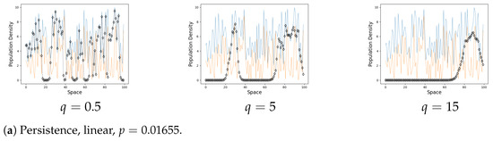
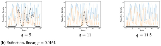
Figure 2. On the graphs the black line represents the population on each site when $t=200$. The blue line is a carrying capacity of each site. The orange line is an Allee threshold of each site. The steady state is generally near the corresponding value of k for a small q, it can drop to 0 on a rare occasion. An increase in the coupling strength q eventually leads to the formation of clusters. The populations of the same cluster tend to align as q increases.

Below are Table 1 with cases which demonstrated persistence and Table 2 with extinct cases for $q=20$ with their last q which gave the persistence, we also may show the distribution for a smaller parameter q. We note that for a better precision in a linear case we have to consider larger qs or more examples because in a quadratic model the absolute value of a coupling term grows faster. Here for the sake of uniformity we have chosen the second option. We begin both tables with the quadratic model as it is simpler in these ranges. We skip some of the examples.

Table 1. Persistence cases. The letter in the index in the column “Which $k^{\left(m\right)},{\beta }^{\left(m\right)}$” represents the dataset we use (L for linear, Q for quadratic), the number represents the iteration, the test dataset is marked by just a number.

Case No.	Model	q	Which ${\mathit{k}}^{\left(\mathit{m}\right)}, {\mathit{\beta }}^{\left(\mathit{m}\right)}$	$\overline{\mathit{k}}$	$\overline{\mathit{\beta }}$	p
1	Quadratic	20	7Q	6.0829	2.7824	0.5180
2	Quadratic	20	8Q	6.3336	2.9024	0.5287
3	Quadratic	20	9Q	6.1039	2.7939	0.5161
4	Linear	5	1	5.9931	2.7475	0.4981
5	Linear	20	1	5.9931	2.7475	0.4981
6	Linear	5	5	6.1951	3.2314	−0.2678
7	Linear	20	5	6.1951	3.2314	−0.2678
8	Linear	5	6L	5.8518	2.9176	0.0166
9	Linear	20	6L	5.8518	2.9176	0.0166
10	Linear	5	9L	5.9594	2.9715	0.0163
11	Linear	20	9L	5.9594	2.9715	0.0163
12	Linear	20	10L	6.1707	3.0772	0.0162
13	Linear	20	11L	5.9465	2.9655	0.0155
14	Linear	5	13L	5.9663	2.9750	0.0163
15	Linear	20	13L	5.9663	2.9750	0.0163
16	Linear	5	14L	5.7967	2.8902	0.0164
17	Linear	20	14L	5.7967	2.8902	0.0164
18	Linear	20	15L	5.8942	2.9389	0.0165
19	Linear	5	17L	6.1019	3.0428	0.0163
20	Linear	20	17L	6.1019	3.0428	0.0163

Table 2. Extinction cases. The letter in the index in the column “Which $k^{\left(m\right)}, {\beta }^{\left(m\right)}$” represents the dataset we use (L for linear, Q for quadratic), the number represents the iteration, the test dataset is marked by just a number. NI marks trivial cases that are not interesting.

Case No.	Model	q	Which ${\mathit{k}}^{\left(\mathit{m}\right)},{\mathit{\beta }}^{\left(\mathit{m}\right)}$	$\overline{\mathit{k}}$	$\overline{\mathit{\beta }}$	p
21	Quadratic	5	1	5.9931	2.7475	0.4981
22	Quadratic	11.5	1	5.9931	2.7475	0.4981
23 (NI)	Quadratic	1.5	2	5.8322	3.2905	−0.7489
24 (NI)	Quadratic	0.5	3	5.9883	3.0180	−0.0477
25 (NI)	Quadratic	1	3	5.9883	3.0180	−0.0477
26 (NI)	Quadratic	3.5	4	6.4793	3.2230	0.0333
27	Quadratic	0.5	5	6.1951	3.2314	−0.2678
28	Quadratic	4.5	5	6.1951	3.2314	−0.2678
29	Quadratic	4.5	6Q	6.0280	2.7574	0.5132
30	Quadratic	7.5	10Q	6.0660	2.7756	0.5147
31	Linear	9.5	2	5.8322	3.2905	−0.7489
32	Linear	5	3	5.9883	3.0180	−0.0477
33	Linear	5	4	6.4792	3.2230	0.0333
34	Linear	13	4	6.4792	3.2230	0.0333
35 (NI)	Linear	13	7L	5.4677	2.7261	0.0156
36	Linear	10	8L	5.9101	2.9469	0.0163
37	Linear	12	8L	5.9101	2.9469	0.0163
38 (NI)	Linear	8.5	12L	5.9783	2.9812	0.0159
39	Linear	5	16L	5.6687	2.8261	0.0164
40	Linear	11	16L	5.6687	2.8261	0.0164

Now we show Figure 3 corresponding to Table 1 and Figure 4 corresponding to Table 2.

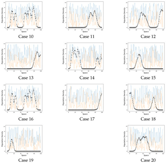
Figure 3. Persistence cases. On the graphs the black line represents the population on each site when $t=200$. The blue line is a carrying capacity of each site. The orange line is an Allee threshold of each site.

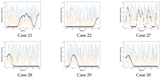
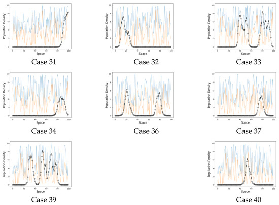
Figure 4. Extinction cases. On the graphs the black line represents the population on each site when $t=200$. The blue line is a carrying capacity of each site. The orange line is an Allee threshold of each site.

6. Discussion and Concluding Remarks

Nature has many complex and fragmented environments and there are still many open theoretical problems [11,12,15,22,32,46,62]; conditions resulting in population collapse and species extinction in a fragmented habitat have long been a focus of the metapopulation theory. Previous research has identified specific factors, such as habitat geometry and demographic/environmental stochasticity, which can contribute to metapopulation collapse under certain conditions [31,32,33,34]. This study aims to contribute to this ongoing discourse by presenting another factor that could potentially result in metapopulation extinction. We investigate a system of arbitrary connected populations; we are primarily concerned with the conditions which correspond to persistaince and extinction.

We first considered a baseline two-patch metapopulation. We continued the research done in [50] giving more sufficient conditions which can be subdivided into a condition on a system type (systems without Allee effect), a condition on extrema of growth functions $f_i$, conditions on q. Then we considered an arbitrary multi-patch system and showed that some of the conditions on q can be extended on the multi-patch system. We showed that the solution to the Cauchy problem exists and is unique, analytic and bounded. We showed that the model belongs to the class of so called monotone dynamical systems, which is very common in mathematical biology [60], and got some important corollaries from that, including another sufficient condition.

We then considered a 1D random metapopulation: a string of patches coupled by a short-distance dispersal (i.e., where each patch is coupled to its immediate neighbours) where the carrying capacity and the Allee threshold of the local population growth is a random function of space and stated a one-parameter sufficient condition. Computer simulations were supported by theoretical results. In particular, Theorem 8 basically tells us that we indeed converge to some steady-state point in Section 4. From the numerical results it can be seen that an increase in coupling may either lead to metapopulation collapse and global species extinction or to the formation of ‘persistence clusters’ (groups of patches where the subpopulations persist) separated by large stretches of empty space where the subpopulations go extinct. We emphasize that the persistence clusters are completely self- organized, as our model does not include any long-distance correlations. A slight change in the vector $\alpha$ causes a slight change in the boundary $p^{*}$ of the parameter $p=\overline{k}-2\overline{\beta }$, so this sufficient coundition is also applicable to more general systems where $\alpha \ne {(1,\dots ,1)}^T$.

Thus, the study of this conceptual model can be considered complete. This paper continues the study done in the paper [50] of the mechanism that may lead to, on one hand, metapopulation extinction or, on the other hand, pattern formation through creating persistence clusters. Although the model used in this paper is very simple, it may give a rise to some important ecological interpretations and stimulate further study. Real ecosystems are usually much more complex: there can be multiple mechanisms; moreover, they can turn on and off independently from each other under specific conditions. A single-species model is typically only applicable on certain timescales [63]. Therefore, it is worth considering more complex models to reveal whether there is similar mechanism as in this model. Despite useful insights from previous work [15,16,19], this issue remains controversial. For example adding other species with some interaction laws to the model may cause the appearence of periodic and chaotic solutions. Coupling different habitats may greatly change the dynamics leading to appearence of new mechanisms or to synchronization of mechanisms between the habitats. All these issues should be studied further in future research.

References

- Ehrlich, P.R.; Ehrlich, A.H. Extinction: The Causes and Consequences of the Disappearance of Species; Ballantine Books: New York, NY, USA, 1985. [Google Scholar]
- Keith, D.A.; Akçakaya, H.R.; Thuiller, W.; Midgley, G.F.; Pearson, R.G.; Phillips, S.J.; Regan, H.M.; Araújo, M.B.; Rebelo, T.G. Predicting extinction risks under climate change: Coupling stochastic population models with dynamic bioclimatic habitat models. Biol. Lett. 2008, 4, 560–563. [Google Scholar] [CrossRef] [PubMed]
- Brooks, T.M.; Mittermeier, R.A.; Mittermeier, C.G.; Da Fonseca, G.A.B.; Rylands, A.B.; Konstant, W.R.; Flick, P.; Pilgrim, J.; Oldfield, S.; Magin, G.; et al. Habitat Loss and Extinction in the Hotspots of Biodiversity. Conserv. Biol. 2002, 16, 909–923. [Google Scholar] [CrossRef]
- Tilman, D.; May, R.M.; Lehman, C.L.; Nowak, M.A. Habitat destruction and the extinction debt. Nature 1994, 371, 65–66. [Google Scholar] [CrossRef]
- Fahrig, L. Relative Effects of Habitat Loss and Fragmentation on Population Extinction. J. Wildl. Manag. 1997, 61, 603–610. [Google Scholar] [CrossRef]
- Wilcox, B.A.; Murphy, D.D. Conservation Strategy: The Effects of Fragmentation on Extinction. Am. Nat. 1985, 125, 879–887. [Google Scholar] [CrossRef]
- Kimura, M. “Stepping Stone” model of population. Ann. Rept. Nat. Inst. Genet. 1953, 3, 62–63. [Google Scholar]
- Renshaw, E. A survey of stepping-stone models in population dynamics. Adv. Appl. Probab. 1986, 18, 581–627. [Google Scholar] [CrossRef]
- Cox, J.T.; Durrett, R. The stepping stone model: New formulas expose old myths. Ann. Appl. Probab. 2002, 12, 1348–1377. [Google Scholar] [CrossRef]
- Jansen, V.A.; Lloyd, A.L. Local stability analysis of spatially homogeneous solutions of multi-patch systems. J. Math. Biol. 2000, 41, 232–252. [Google Scholar] [CrossRef]
- DeAngelis, D.; Zhang, B.; Ni, W.M.; Wang, Y. Carrying Capacity of a Population Diffusing in a Heterogeneous Environment. Mathematics 2020, 8, 49. [Google Scholar] [CrossRef]
- Kareiva, P.; Mullen, A.; Southwood, R. Population Dynamics in Spatially Complex Environments: Theory and Data [and Discussion]. Philos. Trans. Biol. Sci. 1990, 330, 175–190. [Google Scholar]
- Nisbet, R.; Briggs, C.; Gurney, W.; Murdoch, W.; Stewart-Oaten, A. Two-patch metapopulation dynamics. In Patch Dynamics; Springer: Berlin/Heidelberg, Germany, 1993; pp. 125–135. [Google Scholar]
- Blasius, B.; Huppert, A.; Stone, L. Complex dynamics and phase synchronization in spatially extended ecological systems. Nature 1999, 399, 354–359. [Google Scholar] [CrossRef] [PubMed]
- Solé, R.V.; Gamarra, J.G. Chaos, Dispersal and Extinction in Coupled Ecosystems. J. Theor. Biol. 1998, 193, 539–541. [Google Scholar] [CrossRef] [PubMed]
- McCann, K.; Hastings, A.; Harrison, S.; Wilson, W. Population Outbreaks in a Discrete World. Theor. Popul. Biol. 2000, 57, 97–108. [Google Scholar] [CrossRef]
- Amarasekare, P. Allee Effects in Metapopulation Dynamics. Am. Nat. 1998, 152, 298–302. [Google Scholar] [CrossRef]
- Levins, R. Some Demographic and Genetic Consequences of Environmental Heterogeneity for Biological Control1. Bull. Entomol. Soc. Am. 1969, 15, 237–240. [Google Scholar] [CrossRef]
- Levins, R. Extinction. Lectures on Mathmatics in the Life Sciences; American Mathematical Society: Providence, RI, USA, 1970; pp. 77–107. [Google Scholar]
- Pires, M.A.; Duarte Queirós, S.M. Optimal dispersal in ecological dynamics with Allee effect in metapopulations. PLoS ONE 2019, 14, e0218087. [Google Scholar] [CrossRef]
- Wang, W. Population dispersal and Allee effect. Ric. Mat. 2016, 65, 535–548. [Google Scholar] [CrossRef]
- Hanski, I. Metapopulation Ecology; Oxford University Press: Oxford, UK, 1999. [Google Scholar]
- Moran, P.A.P. The statistical analysis of the Canadian Lynx cycle. Aust. J. Zool. 1953, 1, 291–298. [Google Scholar] [CrossRef]
- Royama, T. Analytical Population Dynamics; Chapman & Hall: London, UK, 1992. [Google Scholar]
- Namba, T.; Umemoto, A.; Minami, E. The Effects of Habitat Fragmentation on Persistence of Source–Sink Metapopulations in Systems with Predators and Prey or Apparent Competitors. Theor. Popul. Biol. 1999, 56, 123–137. [Google Scholar] [CrossRef]
- Hanski, I.; Ovaskainen, O. The metapopulation capacity of a fragmented landscape. Nature 2000, 404, 755–758. [Google Scholar] [CrossRef] [PubMed]
- Allen, J.C.; Schaffer, W.M.; Rosko, D. Chaos reduces species extinction by amplifying local population noise. Nature 1993, 364, 229–232. [Google Scholar] [CrossRef] [PubMed]
- Roughgarden, J.; Iwasa, Y. Dynamics of a metapopulation with space-limited subpopulations. Theor. Popul. Biol. 1986, 29, 235–261. [Google Scholar] [CrossRef]
- Bodin, O.; Saura, S. Ranking individual habitat patches as connectivity providers: Integrating network analysis and patch removal experiments. Ecol. Model. 2010, 221, 2393–2405. [Google Scholar] [CrossRef]
- Urban, D.; Keitt, T. Landscape Connectivity: A Graph-Theoretic Perspective. Ecology 2001, 82, 1205–1218. [Google Scholar] [CrossRef]
- Kininmonth, S.; Drechsler, M.; Johst, K.; Possingham, H.P. Metapopulation mean life time within complex networks. Mar. Ecol. Prog. Ser. 2010, 417, 139–149. [Google Scholar] [CrossRef]
- With, K.A.; King, A.W. Extinction Thresholds for Species in Fractal Landscapes. Conserv. Biol. 1999, 13, 314–326. [Google Scholar] [CrossRef]
- Harrison, S.; Quinn, J.F. Correlated Environments and the Persistence of Metapopulations. Oikos 1989, 56, 293–298. [Google Scholar] [CrossRef]
- Legendre, S.; Schoener, T.W.; Clobert, J.; Spiller, D.A. How Is Extinction Risk Related to Population-Size Variability over Time? A Family of Models for Species with Repeated Extinction and Immigration. Am. Nat. 2008, 172, 282–298. [Google Scholar] [CrossRef]
- Croteau, E.K. Causes and Consequences of Dispersal in Plants and Animals. Nat. Educ. Knowl. 2010, 3, 12. [Google Scholar]
- Travis, J.M.J.; Delgado, M.; Bocedi, G.; Baguette, M.; Bartoń, K.; Bonte, D.; Boulangeat, I.; Hodgson, J.A.; Kubisch, A.; Penteriani, V.; et al. Dispersal and species’ responses to climate change. Oikos 2013, 122, 1532–1540. [Google Scholar] [CrossRef]
- Edelstein-Keshet, L. Mathematical Models in Biology; McGraw-Hill: New York, NY, USA, 1988. [Google Scholar]
- Murray, J. Mathematical Biology; Springer: Berlin/Heidelberg, Germany, 1989. [Google Scholar]
- Kot, M. Elements of Mathematical Ecology; Cambridge University Press: Cambridge, UK, 2001. [Google Scholar]
- Dennis, B. Allee Effects: Population Growth, Critical Density, and the Chance of Extinction. Nat. Resour. Model. 1989, 3, 481–538. [Google Scholar] [CrossRef]
- Stephens, P.A.; Sutherland, W.J. Consequences of the Allee effect for behaviour, ecology and conservation. Trends Ecol. Evol. 1999, 14, 401–405. [Google Scholar] [CrossRef] [PubMed]
- Lidicker, W. The Allee Effect: Its History and Future Importance. Open Ecol. J. 2010, 3, 71–82. [Google Scholar] [CrossRef]
- Berec, L. Allee effects under climate change. Oikos 2019, 128, 972–983. [Google Scholar] [CrossRef]
- Courchamp, F.; Berek, L.; Gascoigne, J. Allee Effects in Ecology and Conservation; Oxford University Press: Oxford, MA, USA, 2008. [Google Scholar]
- Lewis, M.; Kareiva, P. Allee Dynamics and the Spread of Invading Organisms. Theor. Popul. Biol. 1993, 43, 141–158. [Google Scholar] [CrossRef]
- Keitt, T.H.; Lewis, M.A.; Holt, R.D. Allee Effects, Invasion Pinning, and Species’ Borders. Am. Nat. 2001, 157, 203–216. [Google Scholar] [CrossRef]
- Boukal, D.S.; Berec, L. Single-species Models of the Allee Effect: Extinction Boundaries, Sex Ratios and Mate Encounters. J. Theor. Biol. 2002, 218, 375–394. [Google Scholar] [CrossRef]
- Sun, G.Q. Mathematical modeling of population dynamics with Allee effect. Nonlinear Dyn. 2016, 85, 1–12. [Google Scholar] [CrossRef]
- Petrovskii, S.; Li, B.L. Increased Coupling Between Subpopulations in a Spatially Structured Environment Can Lead to Population Outbreaks. J. Theor. Biol. 2001, 212, 549–562. [Google Scholar] [CrossRef]
- Althagafi, H.; Petrovskii, S. Metapopulation Persistence and Extinction in a Fragmented Random Habitat: A Simulation Study. Mathematics 2021, 9, 2202. [Google Scholar] [CrossRef]
- SciPy Documentation. Available online: https://docs.scipy.org/doc/scipy/reference/generated/scipy.integrate.solve_ivp.html. (accessed on 12 August 2023).
- Vinberg, E. A Course in Algebra, 2nd ed.; Factorial Press: Moscow, Russia, 2001. (In Russian) [Google Scholar]
- Zorich, V.A. Mathematical Analysis I, 2nd ed.; Universitext; Springer: Berlin/Heidelberg, Germany, 2015. [Google Scholar] [CrossRef]
- Kolmogorov, A.; Fomin, S. Elements of the Theory of Functions and Functional Analysis, 7th ed.; FIZMATLIT: Moscow, Russia, 2004. (In Russian) [Google Scholar]
- Zorich, V.A. Mathematical Analysis II, 2nd ed.; Universitext; Springer: Berlin/Heidelberg, Germany, 2015. [Google Scholar] [CrossRef]
- Kepley, S.; Zhang, T. A constructive proof of the Cauchy–Kovalevskaya theorem for ordinary differential equations. J. Fixed Point Theory Appl. 2021, 23, 7. [Google Scholar] [CrossRef]
- Zeidler, E. Nonlinear Functional Analysis and its Applications. I: Fixed-Point Theorems; Springer: New York, NY, USA, 1986. [Google Scholar]
- Feltrin, G.; Zanolin, F. Equilibrium points, periodic solutions and the Brouwer fixed point theorem for convex and non-convex domains. J. Fixed Point Theory Appl. 2022, 24, 68. [Google Scholar] [CrossRef]
- Bhatia, N.P.; Szego, G.P. Dynamical Systems: Stability Theory and Applications; Springer: Berlin/Heidelberg, Germany, 1967. [Google Scholar]
- Hirsch, M.W.; Smith, H. Monotone Dynamical Systems; Elsevier: Amsterdam, The Netherlands, 2005; Chapter 4. [Google Scholar]
- Ross, S.M. A First Course in Probability, 8th ed.; Pearson Prentice Hall: Upper Saddle River, NJ, USA, 2010. [Google Scholar]
- Seno, H. Effect of a singular patch on population persistence in a multi-patch system. Ecol. Model. 1988, 43, 271–286. [Google Scholar] [CrossRef]
- Ludwig, D.; Jones, D.D.; Holling, C.S. Qualitative Analysis of Insect Outbreak Systems: The Spruce Budworm and Forest. J. Anim. Ecol. 1978, 47, 315–332. [Google Scholar] [CrossRef]
Disclaimer/Publisher’s Note: The statements, opinions and data contained in all publications are solely those of the individual author(s) and contributor(s) and not of MDPI and/or the editor(s). MDPI and/or the editor(s) disclaim responsibility for any injury to people or property resulting from any ideas, methods, instructions or products referred to in the content. |
© 2023 by the authors. Licensee MDPI, Basel, Switzerland. This article is an open access article distributed under the terms and conditions of the Creative Commons Attribution (CC BY) license (https://creativecommons.org/licenses/by/4.0/).