Mean-Field Analysis with Random Perturbations to Detect Gliders in Cellular Automata

Abstract

Cellular automata are mathematical models that represent systems with complex behavior through simple interactions between their individual elements. These models can be used to study unconventional computational systems and complexity. One notable aspect of cellular automata is their ability to create structures known as gliders, which move in a regular pattern to represent the manipulation of information. This paper introduces the modification of mean-field theory applied to cellular automata, using random perturbations based on the system’s evolution rule. The original aspect of this approach is that the perturbation factor is tailored to the nature of the rule, altering the behavior of the mean-field polynomials. By combining the properties of both the original and perturbed polynomials, it is possible to detect when a cellular automaton is more likely to generate gliders without having to run evolutions of the system. This methodology is a useful approach to finding more examples of cellular automata that exhibit complex behavior. We start by examining elementary cellular automata, then move on to examples of automata that can generate gliders with more states. To illustrate the results of this methodology, we provide evolution examples of the detected automata.

1. Introduction

The study of self-reproducing systems capable of self-repairing and carrying out computational processes without the need for a central control unit led to the emergence of cellular automata (CAs). This work was pioneered by John von Neumann and Stanislaw Ulam, and later edited and completed by Arthur W. Burks in [1].

After its inception, cellular automata studies have had numerous facets, primarily benefiting from their easy computational implementation and simple mathematical specifications. This has enabled their modification, adaptation, and application in exploring theoretical concepts like new computational paradigms [2], system reversibility [3], and comprehending how complexity arises from homogeneous elements’ local interaction in a system [4]. These are just a few of the many applications of cellular automata.

The study of cellular automata has experienced significant growth, particularly in the creation of self-reproducing systems from von Neumann’s original 29-state model. The LIFE cellular automaton [5,6] has sparked further investigation into the interaction of structures moving in a fixed background and the creation of complex systems using only a two-state automaton in two dimensions. Additionally, the analysis of elementary cellular automata (ECAs) has been a breakthrough in complexity analysis.

Despite having the simplest computational implementation, they are capable of generating complex behaviors, as noted in [7,8]. ECAs’ computational capabilities are studied in detail in [9], and in [10] it is shown that ECA rule 110 can implement a universal computing system.

Various works have tackled the issue of detecting gliders in cellular automata (CAs). One such method is presented in [11], which automatically filters CA spatiotemporal patterns to identify gliders and related emergent configurations. Another study [12] comprehensively analyzes gliders in ECA rule 54. In [13], a rigorous upper bound on the number of distinct products that gliders can generate is established, particularly for ECA rule 54. Meanwhile, Ref. [14] presents a method that uses genetic programming to search for new cellular automata that can perform computational tasks using gliders. Two variants of particle kinetic models based on CAs and describing two glider species are discussed in [15]. In [16], Ameyalli’s rule, a new two-dimensional CA, is described, featuring an emergent glider gun used to construct logic gates for logical universality. A new system mixing a CA and a genetic algorithm, showing interesting behaviors and glider production, is presented in [17]. Isotropic CAs capable of producing glider-gun and eater dynamics are explained in [18]. In [19], a new approach to duplicating information flows in two-dimensional CAs based on glider-specific collisions capable of simulating logic gates is proposed. In [20], a simple triangular partitioned CA with triangular cells, each divided into three parts, and which is capable of producing gliders, is studied. New tools are introduced in [21] to study self-organization in a family of CAs containing gliders and coalescence properties according to some initial shift-ergodic measures using a limit measure to describe the asymptotic behavior of the CA. Finally, Ref. [22] investigates the use of ECAs and shifting spatiotemporal dynamics of automata-enriching cells with memory to produce complex behaviors.

Research in the detection of cellular automata with complex behaviors is a thriving area of study. The focus is mainly on ECAs, particular cases, and extended models of CAs. However, most of these works use an a posteriori point of view, which means they take a sample of CA evolutions to determine if it can generate gliders in a fixed or periodic background.

Our study uses classical mean-field theory tools and random perturbations to analyze a cellular automaton’s ability to generate gliders in a periodic background without the need for observing multiple evolutions. The proposed method offers specific advantages by eliminating the necessity for running system evolutions to detect glider generation. The evolutions presented in the study only serve to validate the complex dynamics identified by the methodology outlined in this research.

The original aspect of this study involves combining the traditional mean-field approximation method with a new approach that incorporates randomized perturbations into the mean-field polynomials. These perturbations are determined based on the behavior of the CA evolution rule, with a focus on identifying if certain types of neighborhoods occur more frequently than others. The goal is not to enhance the classical mean-field approximation technique, but rather to use it in tandem with a new set of perturbed polynomials in order to identify important criteria for detecting CA rules that can generate gliders.

Several papers have used the mean-field approximation to characterize CAs with gliders, but only for specific cases [23,24,25,26], in conjunction with other analysis tools [11] or limited to ECAs [27,28]. This paper aims to enrich the mean-field approach by identifying CAs with gliders in ECAs and automata with a larger number of states, making it a first attempt of its kind.

Random perturbation of signals has been an active field of research in several mathematics and computer science areas, for example, for the linear tracking of signals [29], for global optimization metaheuristics [30,31], for neural network synchronization [32], for optimal control of a stochastic dynamical system [33], for analyzing the transient dynamics of a predator–prey system [34], for the asymptotic covariance estimation [35], and for the study of the numerical approximation of partial differential equations [36], to mention some representative works. However, to our knowledge, this type of analysis has yet to be applied to detect complex dynamics in CAs.

The density of a CA state can be estimated using classical and perturbed mean-field polynomials, which can then be used to identify high and low classes of densities linked to every state. If the classes identified by the classical polynomials differ from those identified by the perturbed polynomials, it suggests a critical behavior in the CA dynamics. This means that the automaton can have relevant changes in its density of states during its evolution, with the high classes representing a periodic background and the low classes identifying moving structures (or “gliders”) within that background.

This study involves simulating ECAs and one-dimensional CAs with a neighborhood size of two cells, which extends the findings of the study. By utilizing this broad approach, the suggested methodology can be utilized for other CAs with a wider range of states.

The contribution of this study lies in proposing a new methodology capable of detecting mobile structures in a periodic background of a CA with a neighborhood size of 2. The methodology does not require calculating the CA evolutions in advance. This methodology is first applied for the case of ECAs simulated with four-state CAs and two-cell neighborhoods, then applied to CAs with up to nine states.

The paper is structured as follows: In Section 2, a one-dimensional CA, an ECA, and the simulation of all CA using neighborhoods of only two cells are formally described. Section 3 defines mean-field polynomials for CA with a neighborhood size of 2 and applies these polynomials to predict the dynamic behavior of the densities of states for the ECA rule 110. Section 4 explains how a random perturbation is applied to the mean-field polynomials, depending on the evolution rule’s tendency to favor the formation of one neighborhood over others. With this, a methodology is specified to detect CAs forming gliders in a periodic background, based on the analysis of the evolution rule using the classical and perturbed mean-field polynomials. In Section 5, the methodology is applied to CAs, presenting evolutions of CAs capable of generating gliders. Section 6 applies this methodology to CAs with a larger number of states, showing examples of CAs capable of producing complex behaviors. Finally, Section 7 provides the conclusions of this work.

2. Preliminaries of Cellular Automata

This paper will focus on the study of cellular automata in one dimension. A cellular automaton (CA) is defined by three main components: a set of states S, a neighborhood radius r, and an evolution rule, denoted as $\phi :S^{2r+1}\to S$. The CA takes an initial configuration or condition $c^0:{\mathbb{Z}}_m\to S$, where $c^0$ is a one-dimensional array consisting of m cells, with each cell assigned a state from S. The cell at position i is represented by $c_i^0$.

To understand the dynamics of cellular automata (CA), a block of states is defined as $w_i=\{c_{i-r}^0\dots c_{i+r}^0\}$, which consists of r neighboring cells both to the left and right of each $c_i^0$. Using this information, the new state $c_i^1$ is determined through $\phi \left(w_i\right)$. To ensure that the number of cells in $c^1$ is m, periodic boundary conditions are applied. The evolution rule $\phi$ creates a global mapping $\mathsf{\Phi }:c^j\to c^{j+1}$ between configurations, which defines the overall dynamics of the CA. An elementary cellular automaton (ECA) is the simplest type of CA capable of generating complex behaviors. In this case, $\left|S\right|=2$ and $r=1$.

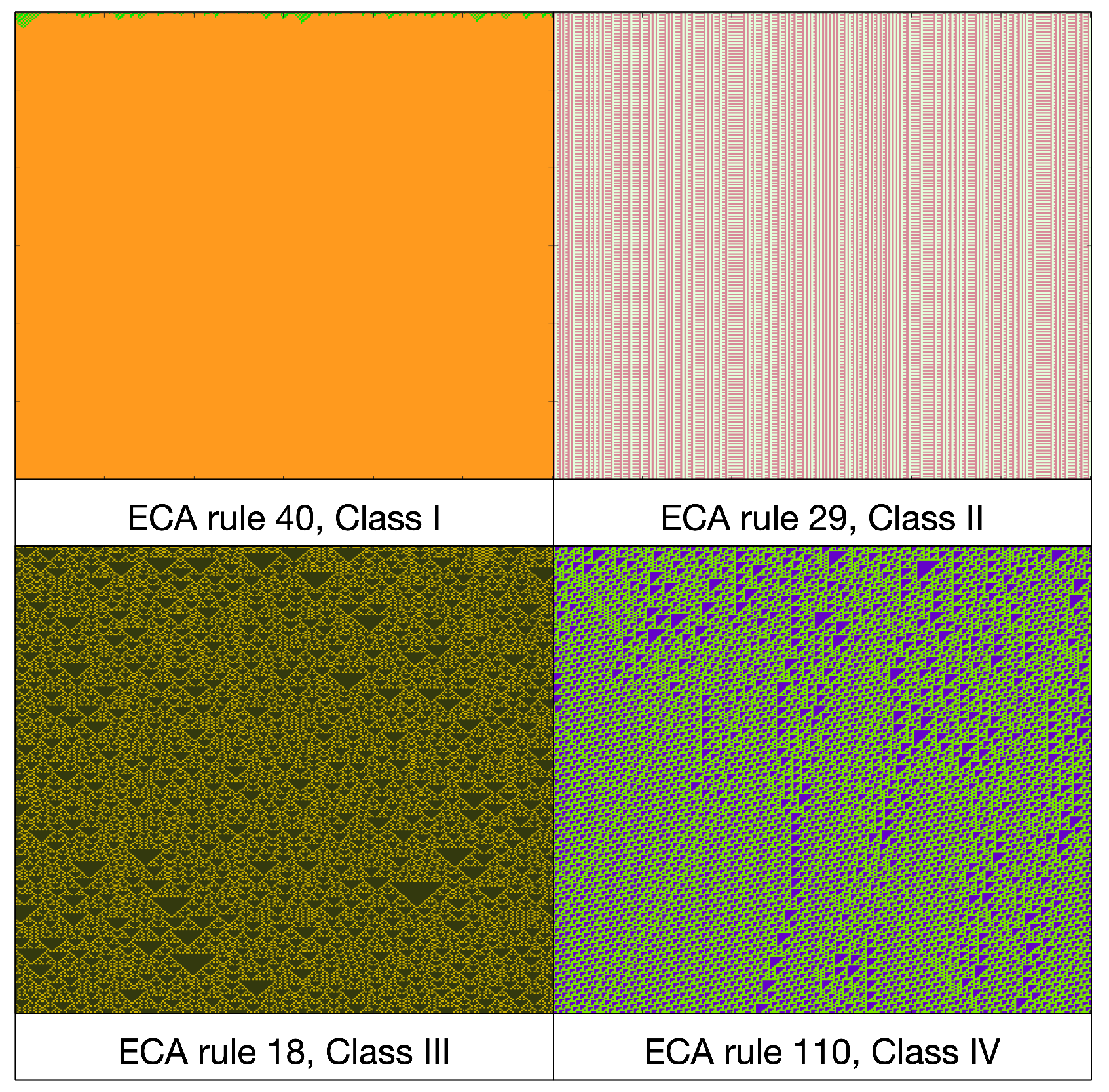
ECAs are widely studied due to their simplicity and the variety of dynamics they can produce. These dynamics can range from fixed or periodic global states to chaotic and complex behaviors. Various classifications have been proposed to categorize the dynamics of ECAs. The most well-known classification is the one by Wolfram, which defines four classes based on the observed dynamics of ECAs. These classes include Class I, which generates a fixed global state, Class II, which produces a periodic global state, Class III, which exhibits chaotic behavior, and Class IV, which results in complex evolutions [37]. To illustrate each class, Figure 1 displays an example of each class using $m=300$ and 300 evolutions.

Complexity in cellular automata (CAs) is a blend of order and chaos. The automaton’s evolution creates a stable or repeating background with moving structures called gliders. These gliders interact with one another, either cancelling each other out, creating a different type of glider, or remaining preserved. Complex cellular automata (CAs) rely on a delicate balance between two defining characteristics: periodicity and chaos. This balance ensures that neither characteristic becomes dominant. Gliders can represent information in these CAs, and logical operators can be implemented through their interactions to enforce a computing process. One-dimensional CAs have a unique property where any CA can be simulated using another CA with a neighborhood size of 2, even if it requires a significant increase in the number of states.

For a CA with a neighborhood radius of r, $\left|S\right|$ states and $\phi :S^{2r+1}\to S$ evolution rule, extending the action of $\phi$ on $S^n$ produces sequences in $S^{n-2r}$ for $n>2r$. By extending the definition of $\phi$, one can map $\phi :S^{2r+2r}\to S^{2r}$. Therefore, we can use a new set of states W with $|S^{2r}|$ states, and $\phi :W^2\to W$ to simulate a CA with $\left|S\right|$ states and a neighborhood size of 2r + 1. It is customary that the evolution of each neighborhood is centered on the following configuration for the new automaton.

While this process has an exponential growth rate that depends on r in the number of new set states, it is advantageous because the results obtained using CAs with a neighborhood size of 2 can be generalized to all other cases.

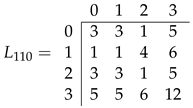
To simulate ECAs, we can use four state CAs. We will use the example of ECA rule 110 shown in Figure 2. In Figure 2A, the neighborhoods with three cells are on the left, and the evolution of the center cell in the next generation is on the right. In Figure 2B, we observe the sequences of four states and their evolutions using $\phi$. In Figure 2C, sequences of two states are renamed as follows: $00\to 0$, $01\to 1$, $10\to 2$, and $11\to 3$; this results in a new state set $W=\{0,\dots ,3\}$. Finally, in (D), we reordered the new evolution rule in matrix form, where the row and column indices are the states of W, and each entry $(w_1,w_2)$ shows the evolution of each sequence $w_1{w}_2\in W^2$. 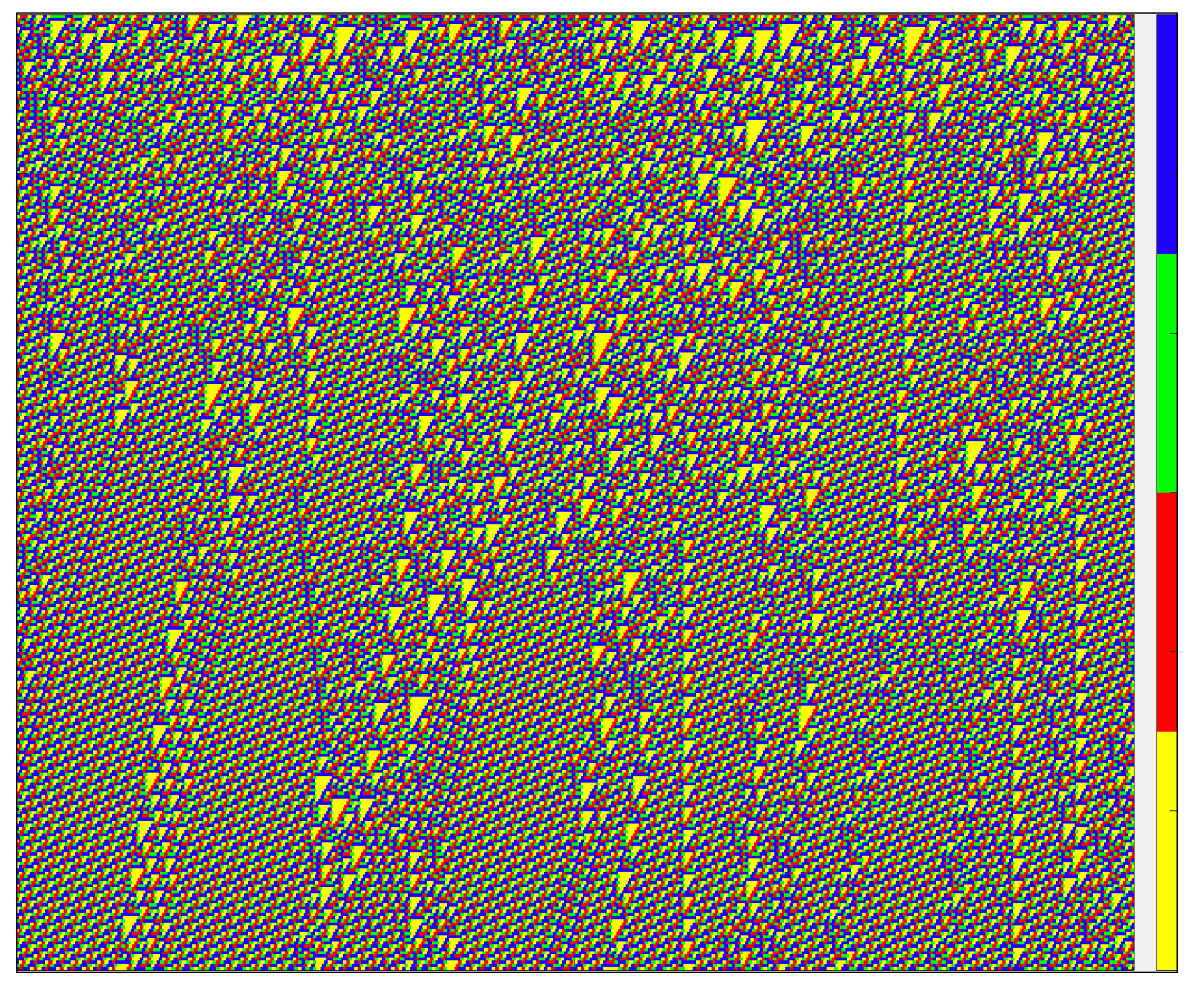Figure 3 shows an evolution of the CA that simulates the ECA rule 110.

3. Mean-Field Analysis

One method of studying the dynamic behavior of a CA is by using mean-field theory. This involves utilizing polynomials that describe how the densities of CA states change based on previous densities, in an iterative manner [38,39]. This approach is advantageous due to its ease of implementation, as the polynomials only require initial values to calculate subsequent densities. However, a disadvantage is that the polynomials tend to quickly converge to an average density, losing the small fluctuations that can occur in the CA evolutions and may indicate complex dynamics.

Here is an example of how to define mean-field polynomials for a CA with a neighborhood size of 2 and $\left|S\right|=4$. To define the polynomial for each density state, we will start by looking at the set $X=S^2$ of all possible neighborhoods such as $\{00,01,02,03,\dots ,33\}$. For $s\in S$, let $d_s^0$ be the initial density of state s in $c^0$, which can be found experimentally as:

$$d_s^0=\frac{{\sum }_{i=1}^m\alpha (c_i^0,s)}{m}$$

(1)

where

$$\alpha (c_i^0,s)=\left\{\begin{array}{cc}1\hfill & \mathrm{iff} c_i^0=s\hfill \\ 0\hfill & \mathrm{in} \mathrm{other} \mathrm{cases}\hfill \end{array}\right.$$

(2)

Using the neighborhoods in X, we will have four mean-field polynomials; one for each state, whose general definition is:

$$p\left(d_s^{k+1}\right)=\sum _{x\in X}\beta (x,s)d_x^k$$

(3)

with

$$\beta (x,s)=\left\{\begin{array}{cc}1\hfill & \mathrm{iff} \phi \left(x\right)=s\hfill \\ 0\hfill & \mathrm{in} \mathrm{other} \mathrm{cases}\hfill \end{array}\right.$$

(4)

where $k\ge 0$ denotes the iteration step of the polynomial and $d_x^k$ is the estimated density of the neighborhood x in the $c^k$ configuration. If we start by defining $c^0$ randomly, we can assume that each state in $c^0$ occurs independently. This is because the process approximates a Bernoulli distribution. Therefore, for any $x=s_i{s}_j$, we can calculate $d_x^0$ as $d_{s_i}^0{d}_{s_j}^0$, where $0\le i,j\le 3$, and $s_i\in S$. We can repeat this assumption for all subsequent values of k which makes calculations simpler using mean-field approximation.

The mean-field polynomials satisfy that ${\sum }_{s\in S}p\left(d_s^k\right)=1$, $\forall k\ge 0$. It is important to note that the independence of state occurrences in a configuration is justified when it is randomly defined. Polynomials are useful for calculating a decent approximation of density behavior, especially when configurations have a larger number of cells. However, this definition of polynomials may not fully capture the behavior of densities, especially in complex CA.

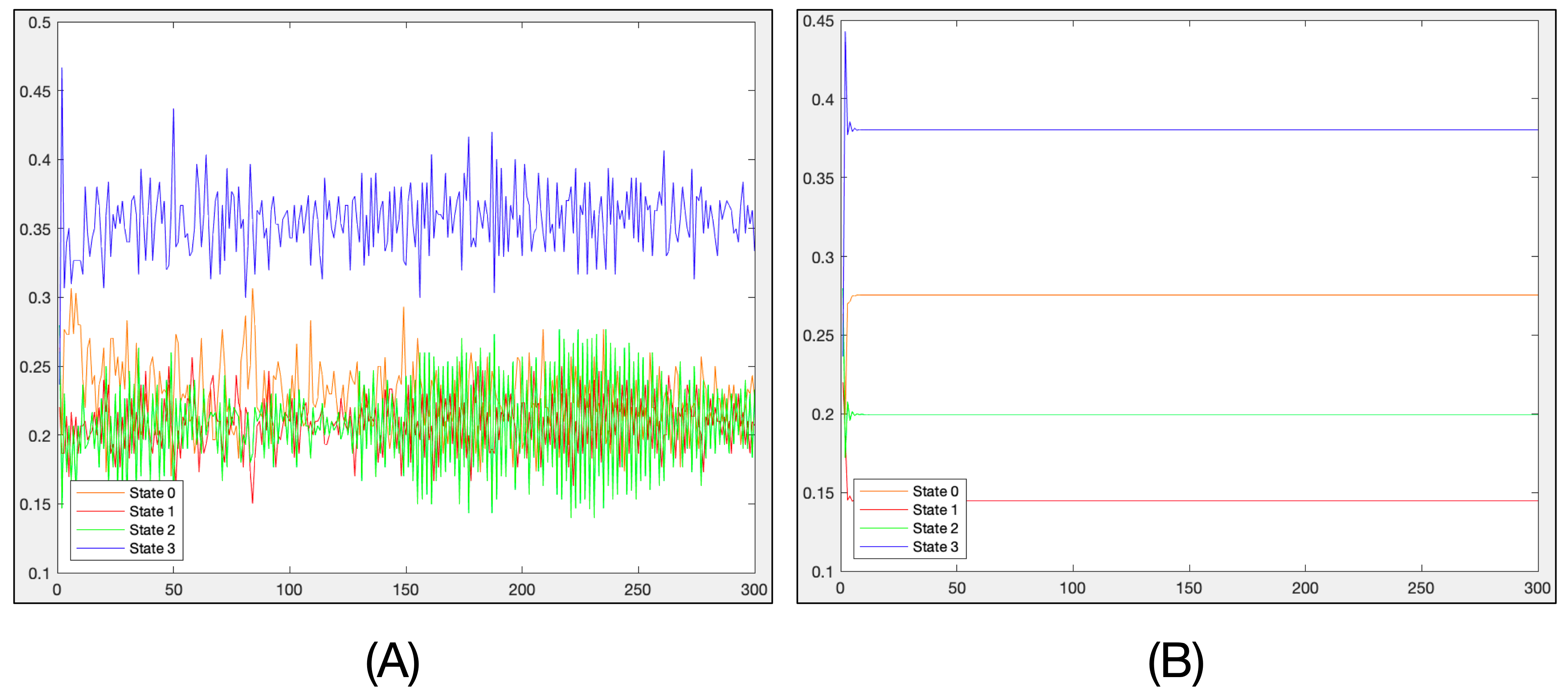
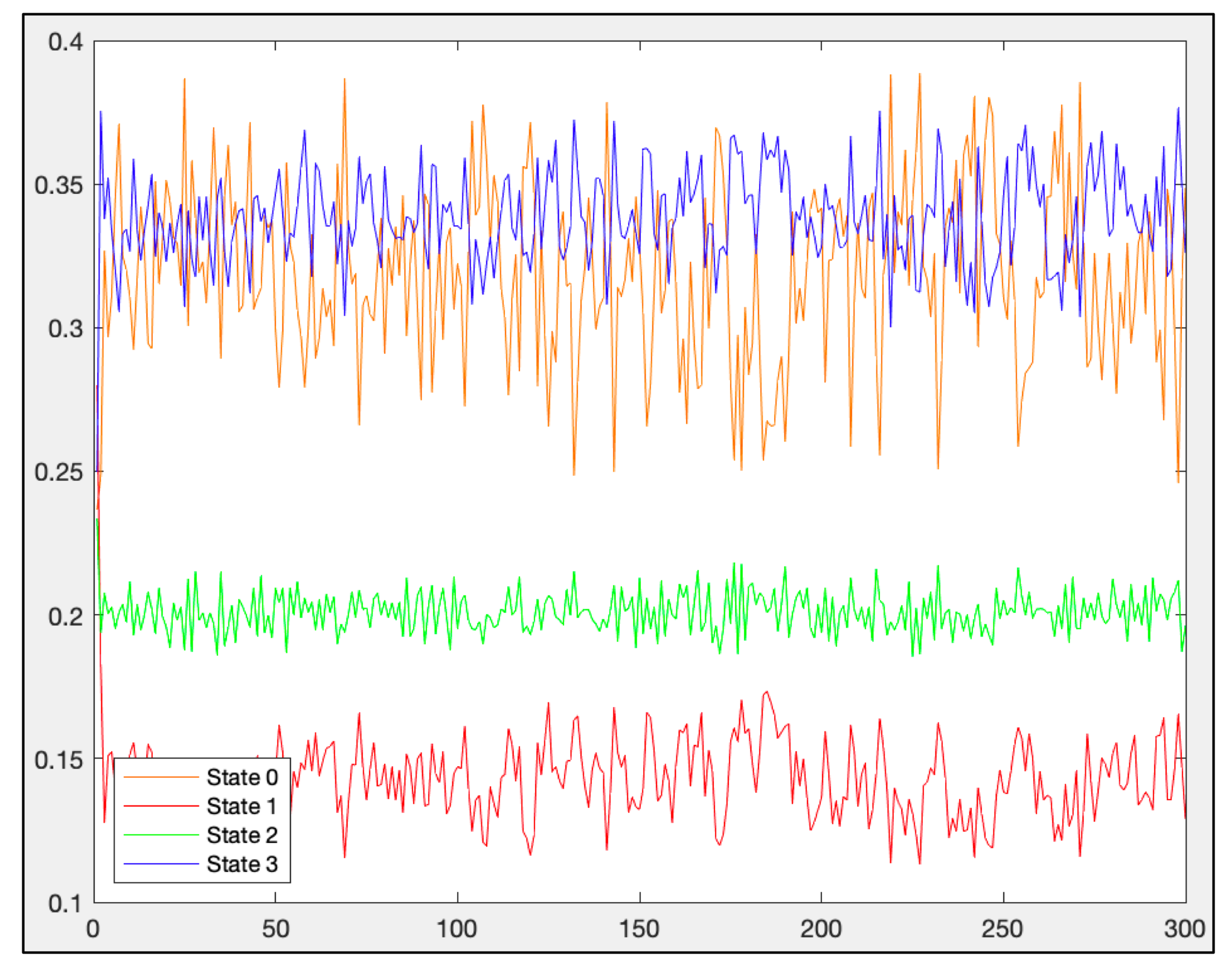
For instance, consider the CA of four states presented in Figure 2 that emulates the ECA rule 110. In Figure 4A, we can observe the experimental density of the CA when $m=300$ and 300 evolutions. Additionally, Figure 4B shows the corresponding approximation calculated by the mean-field polynomials.

We can observe from Figure 4 that while the mean-field polynomials defined in Equation (3) provide a good approximation of the mean density, they quickly reach a fixed value. In Figure 4B, the highest estimated density belongs to the 3 state, followed by the density of the 0 state, while the other states have lower estimated densities. However, experimentally, the densities of the states 0 to 2 are similar.

This reveals that mean-field polynomials can provide initial information to identify a complex CA. States with higher densities work to create periodic backgrounds, while the remaining states form gliders. Thus, a first filter to determine if a CA is complex is to check its estimated densities. If the densities are not very high (less than $0.5$) and are heterogeneous, meaning they have two distinct classes of states, with one having higher densities and the other having slight but not negligible densities (greater than $0.1$), then the CA may be able to yield complex behaviors.

4. Random Perturbation of Mean-Field Analysis

In the previous section, it was noted that the estimation of mean-field polynomials needs to be more accurate for determining the densities of states in complex CAs. Although the estimation yields two states with higher density, the experimental part shows a dominant density and others with a similar, lower density. To complement this analysis and identify whether a CA can generate complex behaviors, random perturbations are applied to the mean-field polynomials. This is performed to test the robustness of the polynomials in maintaining their high- and low-density classes. If the density estimations remain stable when small random perturbations are applied, it would indicate that the polynomials define very stable dynamics.

However, if small random perturbations cause a significant change in the polynomial estimation, such as the high-density classes being different in the original polynomials than in the perturbed polynomials, then the density dynamics are sensitive to these perturbations. This is when we can detect CAs with complex behavior.

The mean-field polynomials with random perturbations will be defined as follows:

$$d_s^{k+1}=q\left(d_s^k\right)=\sum _{x\in X}\gamma g\left(x\right)d_x^k$$

(5)

where $g\left(x\right)$ is a factor representing the tendency the evolution rule $\phi$ has to produce the neighborhood x in a CA, and $\gamma$ is a random number between 0 and ${\gamma }_{max}$.

The factor $g\left(x\right)$ depends directly on $\phi$ and is calculated as follows:

• For each element x in the set X, count the number of ancestral sequences $l_x$. Here, $l_x$ refers to the number of sequences w in $S^3$ such that $\phi \left(w\right)=x$.
• For each $x\in X$, the average number of ancestors can be calculated as ${\left|S\right|}^3/{\left|S\right|}^2=\left|S\right|$. If $l_x>\left|S\right|$, it is assumed that the $\phi$ evolution rule promotes the emergence of the x-neighborhood, while if $l_x<\left|S\right|$, it is said to discourage it.
• We define a tendency matrix M of order $\left|S\right|\times \left|S\right|$ such that each entry $m_{i,j}=\frac{l_x-\left|S\right|}{\left|S\right|}$ for all $i,j\in S$ and $x=ij$.
• Finally $g\left(x\right)=m_{i,j}$ for $x=ij$.

Finally, the random value $\gamma$ is a weighting factor for applying $g\left(x\right)$ to each density in Equation (5); in this study, we take $\gamma =0.75$.

The concept behind $g\left(x\right)$ is to assign a value of zero to the neighborhood x if it has an average number of ancestors. However, if the evolution rule favors or does not favor its formation based on the average value, $g\left(x\right)$ will have a positive or negative value. The purpose of incorporating an extra step in the computation of $l_x$ is to enhance the accuracy in the neighborhoods that the evolution rule tends to generate. This step helps in determining the random perturbations in the density of neighborhoods which are used as the foundation for calculating the mean-field approximation.

To apply $g\left(x\right)$ to each density in Equation (5), a random value called $\gamma$ is used as a weighting factor. In this study, we have chosen to use $\gamma =0.75$.

In order to maintain that ${\sum }_{s\in S}q\left(d_s^k\right)=1$, $\forall k\ge 0$ after applying the perturbations $\gamma g\left(x\right)$, we take the difference

$$e=\frac{1-{\sum }_{s\in S}q\left(d_s^k\right)}{\left|S\right|}$$

(6)

We update $d_s^k=d_s^k+e$, $\forall s\in S$. After perturbing and normalizing the polynomials, we can recalculate the densities $d_s$ through an iterative process. This results in two sets of densities: the first set obtained using the classical polynomials (refer to Equation (3)), and the second set estimated using Equations (5) and (6).

We will be utilizing both types of polynomials to detect CAs that have gliders in a periodic background. To do this, we will classify the states as either belonging to a high-estimated density class or a low-estimated density class.

• For each $s\in S$ we compute the average densities $\overline{d_s}$ after m iterations.
• The highest density ${\overline{d}}_{max}$ defines the first state s in the high-density ${\mathcal{C}}_{high}$ class.
• For $\delta ={\overline{d}}_{max}-ϵ$ the remaining densities $\overline{d_s}>=\delta$ define the remaining states in ${\mathcal{C}}_{high}$.
• The rest of the states define the class ${\mathcal{C}}_{low}$ with low densities.

In this work, we will set $ϵ$ to 0.15 for differences between ${\mathcal{C}}_{high}$ and ${\mathcal{C}}_{low}$. Using classical and perturbed polynomials, we obtain two pairs of classes: ${\mathcal{C}}_{high}^c$ and ${\mathcal{C}}_{low}^c$ from classical polynomials, and ${\mathcal{C}}_{high}^p$ and ${\mathcal{C}}_{low}^p$ from perturbed polynomials. These classes will determine the parameters needed to identify potential CAs yielding gliders.

• The maximum densities in ${\mathcal{C}}_{high}^c$ and ${\mathcal{C}}_{high}^p$ must not exceed $0.5$.
• $|{\mathcal{C}}_{high}^c|\ne |{\mathcal{C}}_{high}^p|$.
• $|{\mathcal{C}}_{low}^c|>0$ and $|{\mathcal{C}}_{low}^p|>0$.

5. Experiments with ECAs

To test the methodology explained in the previous section, we first took all ECAs from rule 0 to rule 255. Each ECA is first simulated with a CA of 4 states and 2 neighborhood size, and on this rule, the mean-field polynomials, both classical and randomly perturbed, were applied depending on the rule trends.

For the case of the 110 rule, the 64 sequences of 3 states and their evolutions were taken. Let us use $L_{110}$ as the matrix showing the number of ancestor sequences of each x neighborhood where each entry $(i,j)$ in $L_{110}$ is equal to $l_x$ for $x=ij$.

In order to test the methodology described in the previous section, we examined all ECAs from rule 0 to rule 255. Each ECA was simulated using a CA with 4 states and a neighborhood size of 2. Mean-field polynomials, both classical and randomly perturbed, were then applied based on the trends of each rule.

For the specific case of rule 110, we analyzed the 64 sequences of 3 states and their corresponding evolutions. We used a matrix called $L_{110}$ to represent the number of ancestor sequences for each x neighborhood, where each entry $(i,j)$ in $L_{110}$ is equal to $l_x$ for $x=ij$.

(7)

Taking $L_{110}$, the matrix $M_{110}$ is obtained by taking $\frac{L_{110}-4}{4}$.

(8)

Using the elements of matrix $M_{110}$, we apply random perturbations to mean-field polynomials in Equation (5) and normalize them with Equation (6). Figure 5 illustrates the behavior of estimated densities under this scheme.

Referring to Figure 4B and Figure 5, and following the class detection method explained in Section 4, we can determine that ${\mathcal{C}}_{high}^c=\left\{3\right\}$, ${\mathcal{C}}_{low}^c=\{0,1,2\}$, ${\mathcal{C}}_{high}^p=\{0,3\}$ y ${\mathcal{C}}_{low}^p=\{1,2\}$. These classes indicate that mean-field polynomials display critical behavior when subjected to random perturbations, suggesting their ability to generate gliders during their evolution.

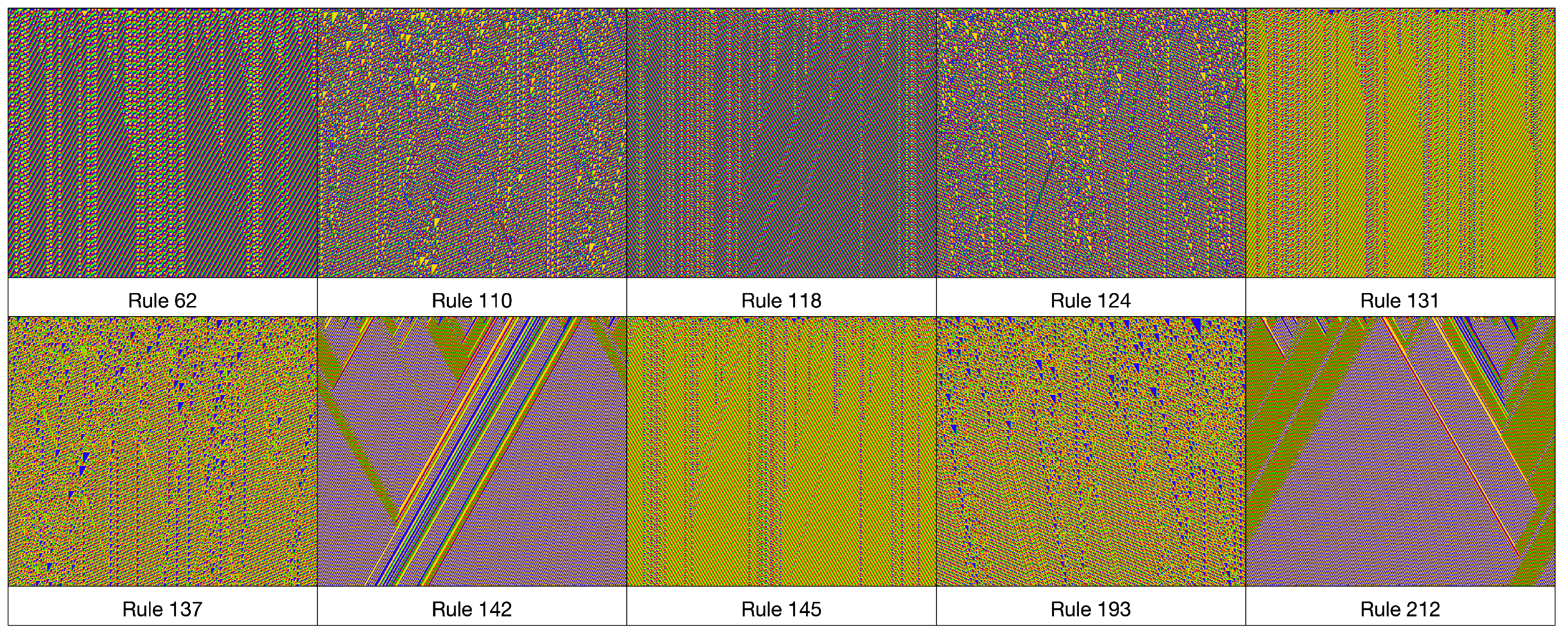
Figure 6 illustrates the ECAs identified as capable of generating gliders in a periodic background. This was determined by simulating them as 4-state CAs and using the criteria specified in the final part of Section 4, which involves classical and randomly perturbed mean-field polynomials.

6. Experiments with a Higher Number of States

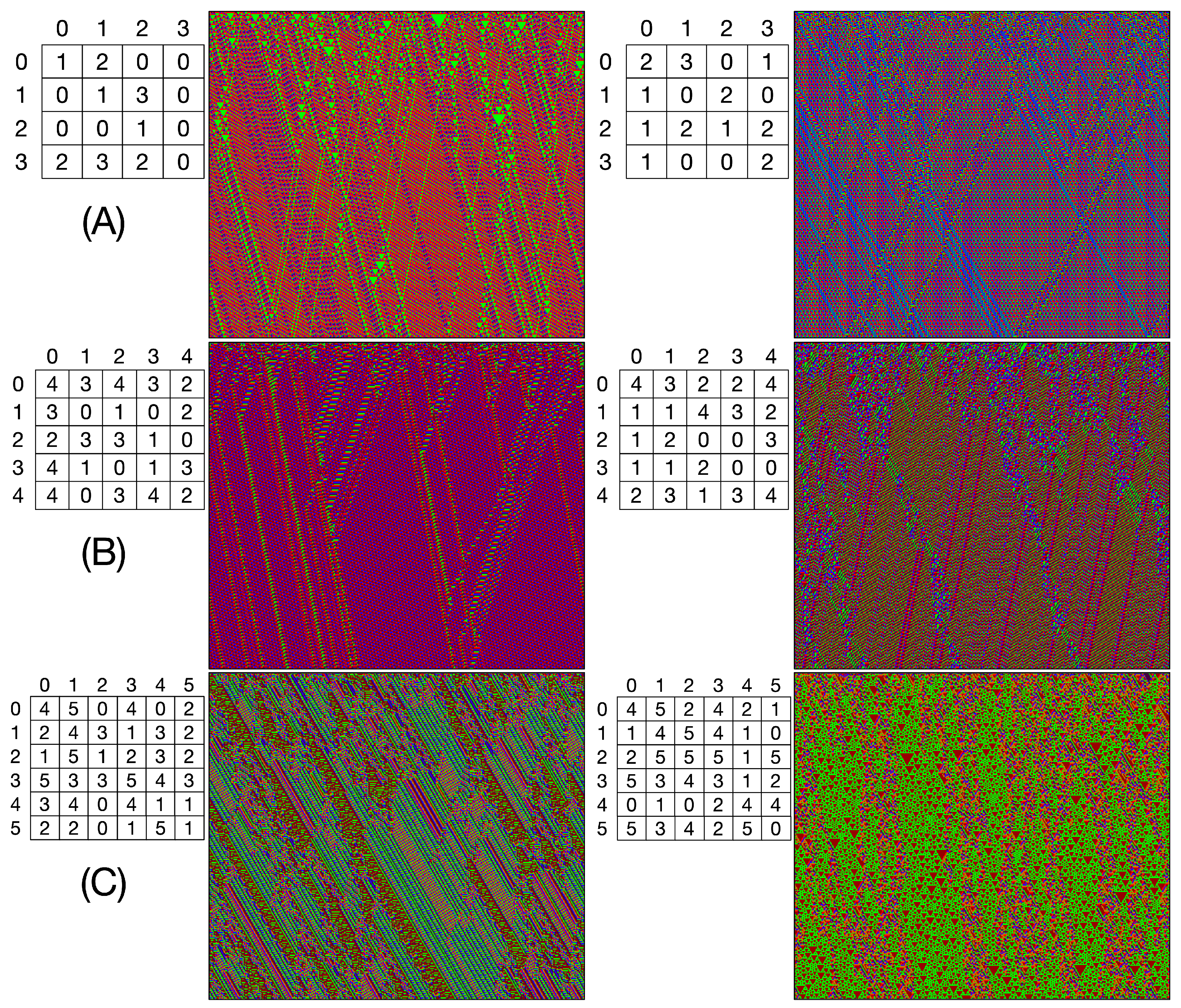
We then modified the method to identify CAs that can generate gliders with 4 to 9 states and a neighborhood size 2. Figure 7 displays two examples for each case, including 4 states (A), 5 states (B), and 6 states (C). The matrix form of the evolution rule is also provided for each case.

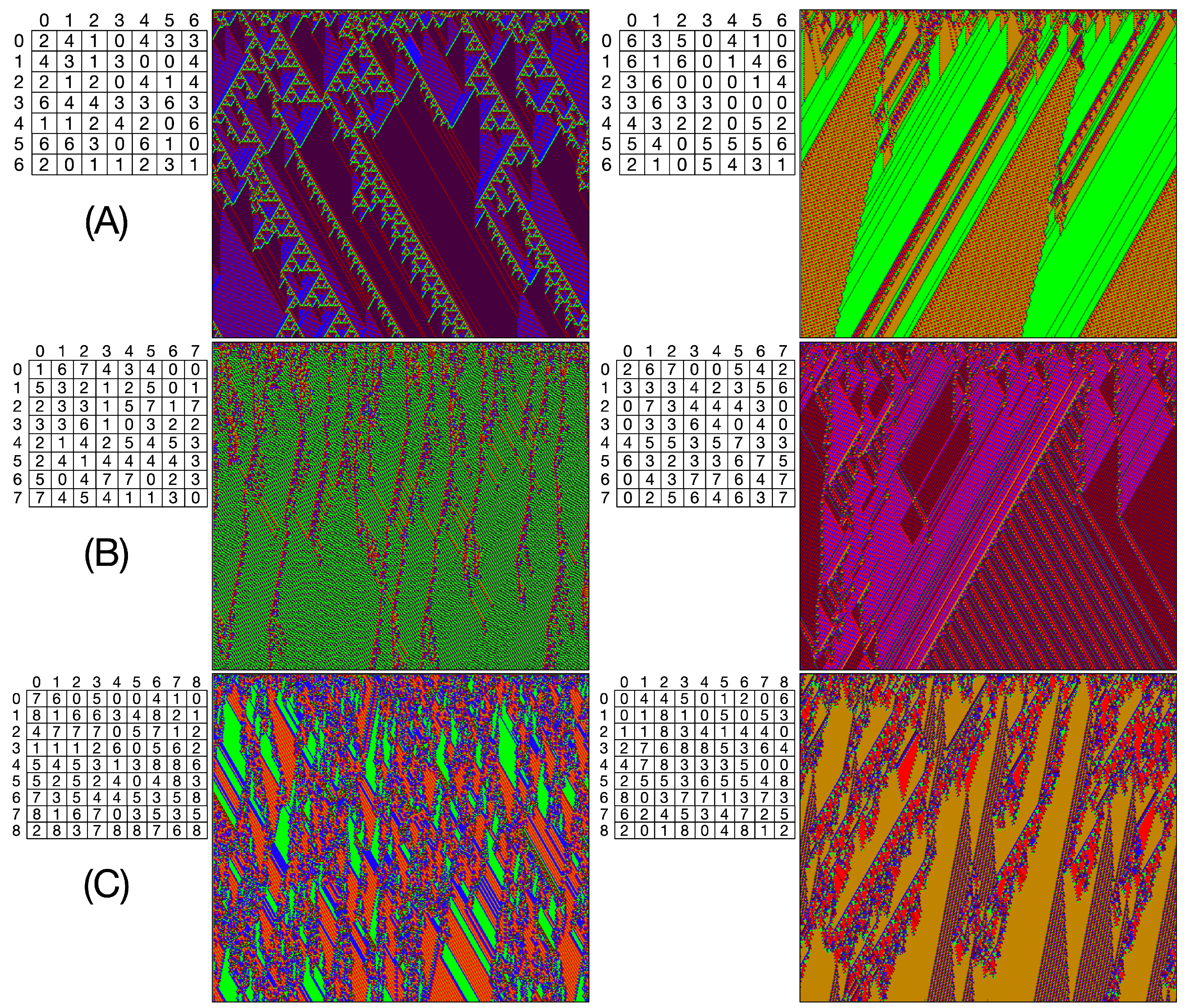
Figure 8 shows examples for 7, 8, and 9 states ((A), (B), and (C), respectively), including their associated evolution rules.

7. Conclusions

In this paper, a straightforward approach to detecting CAs that can produce gliders in a periodic background using mean-field classical polynomials and randomly perturbed polynomials has been presented. The trends of the evolution rule to produce each neighborhood have been considered.

The significant contribution of this work is the detection of CAs capable of generating gliders without the need to observe the automaton’s evolutions but by analyzing its evolution rule. The methodology has been applied to simulated ECAs with four-state CAs and then extended to CAs with from four to nine states, revealing some fascinating specimens that can generate gliders in a periodic background.

This is an initial effort to incorporate random perturbations in addition to the traditional mean-field approximation to identify CAs with gliders. As a result, several parameters in the methodology were fine-tuned through computational experimentation. One potential future work could be to automatically adjust the parameters that define the use of random perturbations. Moreover, this methodology needs further refinement to detect CAs with more complex behavior accurately, for instance, for CAs with a quasi-periodic background, as in the case of the ECA rule 54.

Future work that may arise from this research includes the application of other ways of extending mean-field polynomials to account for a more significant number of densities. It would be worth comparing all proposals that use mean-field approximation to detect gliders and other interesting dynamics in CAs, with the aim of highlighting the benefits, limitations, and research trends of this tool, or working on the state independence assumption in a different way, such as using Bayesian probability. To calculate the tendency matrix for a given evolution rule, we use additive scaling to avoid changes when a neighborhood has the same number of ancestors as the expected average. In future research, it may be worth exploring other forms of normalization, such as multiplicative ones, to improve the modeling of the evolution rule tendency in generating neighborhoods. The use of deep learning computational tools that better model the production of states and sequences of a CA is another possibility to continue this research.