Article

Numerical Computation of Distributions in Finite-State Inhomogeneous Continuous Time Markov Chains, Based on Ergodicity Bounds and Piecewise Constant Approximation

1
Department of Applied Mathematics, Vologda State University, 160000 Vologda, Russia
2
Federal Research Center “Computer Science and Control” of the Russian Academy of Sciences, 119133 Moscow, Russia
3
Vologda Research Center, Russian Academy of Sciences, 160014 Vologda, Russia
4
Moscow Center for Fundamental and Applied Mathematics, Moscow State University, 119991 Moscow, Russia
*
Author to whom correspondence should be addressed.
Mathematics 2023, 11(20), 4265; https://doi.org/10.3390/math11204265
Submission received: 13 September 2023 / Revised: 3 October 2023 / Accepted: 9 October 2023 / Published: 12 October 2023
(This article belongs to the Special Issue Stochastic Processes: Theory, Simulation and Applications)

Abstract

:
In this paper it is shown, that if a possibly inhomogeneous Markov chain with continuous time and finite state space is weakly ergodic and all the entries of its intensity matrix are locally integrable, then, using available results from the perturbation theory, its time-dependent probability characteristics can be approximately obtained from another Markov chain, having piecewise constant intensities and the same state space. The approximation error (the taxicab distance between the state probability distributions) is provided. It is shown how the Cauchy operator and the state probability distribution for an arbitrary initial condition can be calculated. The findings are illustrated with the numerical examples.

1. Introduction

Operations research possesses a great deal of applications for which continuous-time Markov chains (CTMC) with discrete state space serve as adequate mathematical models (see, for example, [1] (Section 5) and [2]). The scope of use of CTMC is broadened if one allows for inhomogeneity, i.e., if one allows some (or all) transition intensities to be non-random functions of time and depend on the state of the chain. A large body of works exists on the analysis of inhomogeneous CTMCs, which covers all the vital questions: existence, numerical solution, asymptotics, and approximations (for a systematic view see, for example, [1] and [3] (Sections 1 and 1.2)).
In this paper, we revisit the problem of the computation of the time-dependent probability distributions of inhomogeneous CTMCs. It is well-known that for such chains analytical solutions are usually not possible and one must resort to other approaches. There exist various techniques to calculate performance measures for CTMCs (See, for example, [4] (Introduction) and [5,6], for a short review related to queuing theory): point-wise stationary approximation [7], uniformization [8,9], heavy-traffic approximation [10,11], robust optimization [3] (Section 2), Monte Carlo simulation, stationary independent period by period approach, state-space enrichment, etc. Probably the most widely applicable technique (or at least popular currently due to the increasing computer power) is comprised of numerical methods for systems of ordinary differential equations (ODEs) [12,13,14,15,16]. In this paper the novel variation of the method for the computation of the Cauchy matrix is proposed for the case when the intensity matrix of a Markov chain is time–dependent. The main requirement for the method to work is that the Markov chain under consideration is weakly ergodic and the entries of its intensity matrix are locally integrable. If these conditions are satisfied then the (approximate) computation of the main characteristics of the chain can be brought down to the computation of those in another chain with the intensity matrix, having piecewise-constant entries. This method is, of course, not new and can be found already in [17]. The main contribution of this paper comes from the observation that the new chain can be considered as the perturbed version of the original chain. Therefore, the estimates for perturbed chains available from the literature can be used (see [18]). Thus, if the chains start from the same state, then the “difference” between them (in l 1 -norm) for any time t > 0 does not exceed the constant, obtained here for the first time in the literature (see (7)). Since exact solutions are rarely available, here we show what difference in the solutions can be expected (see (6)): the main contribution into the approximation error comes from approximate computation of the Cauchy operators (see (17)). These effects are illustrated in the numerical section. Here, a comparison is made with the well-known Runge–Kutta method: the numerical results show that the performance (with respect to the accuracy) is almost identical. Finally, the new approximation method can be executed in parallel and therefore can be efficiently used in a chain with a large number of states.
The paper is structured as follows. In the next section, the preliminary notation and the required definitions are given. Section 3 contains the main result of the paper, i.e., the bounds for the difference between the two chains, original with time-varying intensities and the new one with the piecewise constant intensities. Section 4 discusses the solution algorithm, which is illustrated in the Section 5 with three numerical examples. In the concluding section, a summary and further direction of research is given.

2. Preliminaries

Let X ( t ) , t 0 , be, in general, an inhomogeneous continuous-time Markov chain with a finite or countable state space E S = 0 , 1 , , S , S < . The transition probabilities for X ( t ) will be denoted p i j ( s , t ) = Pr X ( t ) = j X ( s ) = i , i , j 0 , 0 s t . Let p i ( t ) = Pr X ( t ) = i be the state probabilities of the chain and p ( t ) = p 0 ( t ) , p 1 ( t ) , T be the corresponding vector of state probabilities. In what follows, it is assumed that
Pr X t + h = j | X t = i = q i j t h + α i j t , h , i f   j i 1 k i q i k t h + α i t , h , i f   j = i ,
where all α i ( t , h ) are o ( h ) uniformly in i, that is, sup i | α i ( t , h ) | = o ( h ) . Moreover, if X ( t ) is inhomogeneous, then all its infinitesimal characteristics (intensity functions) q i j t are integrable in t on any interval [ a , b ] , 0 a b .
Denote a i j ( t ) = q j i ( t ) for j i and a i i ( t ) = j i a j i ( t ) = j i q i j ( t ) . Further, in order to be able to obtain tighter estimates, its is assumed that
| a i i ( t ) | L <
for almost all t 0 . The state probabilities then satisfy the forward Kolmogorov system
d d t p ( t ) = A ( t ) p ( t ) ,
where A ( t ) = Q T ( t ) , and Q ( t ) is the infinitesimal matrix of the process.
Let · be the usual l 1 -norm, i.e., x = | x i | , and B = sup j i | b i j | for B = ( b i j ) i , j = 0 . Denote Ω = x : x l 1 + & x = 1 . Therefore, A ( t ) = 2 sup k a k k ( t ) 2 L for almost all t 0 , and we can apply the results of [19] to Equation (3) in the space l 1 . Namely, in [19] it was shown that the Cauchy problem for Equation (3) has a unique solution for an arbitrary initial condition. Moreover, if p ( s ) Ω , then p ( t ) Ω , for any 0 s t and any initial condition p ( s ) .
By X ¯ = X ¯ ( t ) , we will denote the “perturbed” Markov chain with the same state space, state probabilities p ¯ i ( t ) , transposed infinitesimal matrix A ¯ ( t ) = a ¯ i j ( t ) i , j = 0 and the “perturbations” themselves, that is, the differences between the corresponding “perturbed” and original characteristics will be denoted by a ^ i j ( t ) , A ^ ( t ) .
Let E ( t , k ) = E X ( t ) X ( 0 ) = k be the conditional mean value of X ( t ) at an arbitrary instant t. Recall that a Markov chain X ( t ) is weakly ergodic if p * ( t ) p * * ( t ) 0 as t for any initial condition, and it has the limiting mean ϕ ( t ) if | E ( t , k ) ϕ ( t ) | 0 as t for any k.

3. Estimation through Piecewise Constant Approximation

Consider the system of linear differential equations in the vector-matrix form (3), where all the elements a i j ( t ) of the matrix A ( t ) are locally integrable non-random functions on [ 0 , ) , i.e., | a b a i j ( t ) d t | < for any ( a , b ) [ 0 , ) .
Let T be a real positive number and N be a positive integer. Put h = T / N and denote A ¯ ( t ) = A N T t T N , where x returns the largest integer less than or equal to x. Therefore, A ¯ ( t ) is the transposed intensity matrix, consisting of piecewise constant locally integrable non-random functions on [ 0 , ) , which satisfies the forward Kolmogorov system of equations
d d t p ¯ ( t ) = A ¯ ( t ) p ¯ ( t ) .
The difference between the systems (3) and (4) can be described by [18] (Theorem 1), which repeat below without the proof. The basic idea behind this result is that if one knows the rate of convergence of the original chain X ( t ) , the estimate for the difference between the systems can be calculated as well.
 Theorem 1 
([18]). Let the Markov chain X ( t ) be exponentially weakly ergodic; that is, for any initial conditions p * ( s ) Ω , p * * ( s ) Ω and any s 0 , t s , there holds the inequality
p * ( t ) p * * ( t ) 2 c e b ( t s ) .
Therefore, for the perturbations small enough ( A ( t ) A ¯ ( t ) ε for almost all t 0 ), the perturbed chain X ¯ ( t ) is also exponentially weakly ergodic, and the following perturbation bound takes place:
p ( t ) p ¯ ( t )
p ( s ) p ¯ ( s ) + ( t s ) ε , i f 0 < t s < 1 b ln c 2 , c 2 e b ( t s ) p ( s ) p ¯ ( s ) + 1 b ( ln c 2 + 1 c e b ( t s ) ) ε , i f t s 1 b ln c 2
and
lim sup t p ( t ) p ¯ ( t ) ( 1 + log ( c / 2 ) ) ε b .
Thus, if the uniform grid is used, one can apply the Theorem 1 to estimate the difference between the state vectors of the original system and of the system with the piecewise constant intensities. One can also notice the following. For large perturbations in A ( t ) (large ε ) and low rate of convergence b, the number of steps N must be large to compensate ε and decrease the right-hand side of (6). If one does not pay attention to such differences as (6), which always appear if the piecewise constant matrix replaces the original one, the error in the final result can be severely underestimated.
In what follows, we consider two ways to obtain the estimation of the state vector. One is through the discretization of the intensity matrix and exact solution of the system with constant coefficients. The other is through the discretization of the intensity matrix and the approximate calculation of the Cauchy operator.

4. Estimation of the State Probabilities

 Theorem 2. 
If conditions of the [18] (Theorem 1) are satisfied and p ( 0 ) = p ¯ ( 0 ) , then the following bound holds:
p ( T ) p ¯ ( T ) T ε , i f 0 < T < 1 b ln c 2 , 1 b ( ln c 2 + 1 c e b T ) ε , i f T 1 b ln c 2 .
 Theorem 3. 
If conditions of the [18] (Theorem 1) are satisfied and A ( t ) and A ¯ ( t ) are T-periodic, then the following bound for periodic limiting solutions of the corresponding systems (3) and (4) holds:
sup 0 t T p ( t ) p ¯ ( t ) ( 1 + log ( c / 2 ) ) ε b .
Exact solutions of the system with the constant intensities can (in principle) be found using computer algebra systems. However, as it is demonstrated in Example 1, even in the simplest cases the solution may turn out to be too cumbersome. Therefore, in what follows we dwell on the direct numerical method for the solution of the system and provide the bound of its approximation error. Firstly, from (3) and (4) we have the relations
p ( t ) = U ( t , s ) p ( s )
p ¯ ( t ) = U ¯ ( t , s ) p ¯ ( s )
which imply that
U ¯ ( h ( k + 1 ) , h k ) = U ¯ n ( h ( k + 1 ) , h k ) + G k ,
where G k is a matrix and U ¯ n ( t + h , t ) = I + k = 1 n ( A ¯ ( t ) h ) k k ! . Note that the column-sum of a column in U n ( t ) is always equal to 1 unless n is small; in the latter case, negative values may appear. Therefore, during calculations a non-negativity check is required, otherwise U n ( t ) can become larger than one. Henceforth, we can assume that U ¯ n ( h ( i + 1 ) , h i ) 0 for i and thus U ¯ n ( h ( i + 1 ) , h i ) = 1 .
Let us estimate the approximation error on [ 0 , T ] . By using the Cauchy operator’s property we have
U ¯ ( T , 0 ) = i = 0 N 1 ( U ¯ ( h ( i + 1 ) , h i ) = i = 0 N 1 ( U ¯ n ( h ( i + 1 ) , h i ) + G i ) ,
or, after the expansion and collection of the common terms,
U ¯ ( T , 0 ) = i = 0 N 1 U ¯ n ( h ( i + 1 ) , h i ) + i = 0 N 1 G i k = 0 ; k i N 1 U ¯ n ( h ( k + 1 ) , h k ) +
If one denotes G = max 0 k N 1 G k , then it follows that
U ¯ ( T , 0 ) U ¯ n ( T , 0 ) ( 1 + G ) N 1 .
Therefore, the following theorem holds.
 Theorem 4. 
If conditions of the [18] (Theorem 1), are satisfied, then for sufficiently large n, such that U ¯ n ( h ( i + 1 ) , h i ) 0 , i = 1 , , n , and if p ( 0 ) = p ¯ ( 0 ) , the following bound holds:
p ( T ) p ¯ ( T ) ( 1 + G ) N 1 + T ε , i f 0 < T < 1 b ln c 2 , 1 b ( ln c 2 + 1 c e b T ) ε , i f T 1 b ln c 2 .
Therefore, to construct the Cauchy operator it is sufficient to compute U ¯ n ( t + h , t ) = I + k = 1 n ( A ¯ ( t ) h ) k k ! and U ¯ n ( k h , 0 ) = i = 0 k 1 U ¯ n ( h ( i + 1 ) , h i ) . A specific solution is found by multiplying the Cauchy operator by the initial condition, i.e., p ( k h ) = i = 0 k 1 U ¯ n ( h ( i + 1 ) , h i ) p ( 0 ) . Using the associative property of matrices, and by multiplying them in a proper order, the computation of p ( k h ) can be performed in parallel and thus can be made quite fast. In particular, if A ( t ) contains many non-zero intensities, this method may outperform standard ones (see the Introduction).
What is left is the estimation of G. From (12), it follows that G k = i = n + 1 ( A ( h k ) h ) i i ! . Therefore,
G = max 0 k N 1 G k i = n + 1 ( A ( h k ) h ) i i ! i = n + 1 ( 2 L h ) i i ! = e 2 h L 1 Γ ( n + 1 , 2 h L ) n ! ,
where Γ ( s , x ) denotes the incomplete Gamma function.

5. Numerical Examples

Below, three examples will be considered. Firstly, we consider the example in which the original system is solved with the Runge–Kutta method and the exact solution of the system with a piecewise constant is found. In the second example, we are concerned with the computation of the value of the probability vector at a given time t = T . In the third example, the same computation is carried out, except for the fact that here the intensity matrix A ( t ) does not depend on t. This substantially reduces the approximation error: in the right part of (16), ε becomes equal to 0 (since discretization is no longer needed) and the only error left is due to (15).

5.1. Example 1

In this example, we will build the exact solution and obtain the exact form of the limiting distribution of the process with piecewise constant intensity matrix and compare it (see (20)) with the limiting distribution of the original process with the matrix A ( t ) . Assume a birth-death process has two states and the arrival and death intensities are equal to λ ( t ) = 1 cos ( t ) , μ ( t ) = 5 sin ( t ) , respectively. Break the [ 0 , 2 π ] interval into four intervals of equal length, i.e., the breakpoints are 0 , π 2 , π , 3 π 2 , 2 π . Then N = 4 , h = π 2 , and ε = 2 The solutions of the system (4) in each of the intervals are
p 0 ( t ) = 1 + e 5 t a , p 0 ( t ) = 4 5 + e 5 t b , p 0 ( t ) = 5 7 + e 7 t c , p 0 ( t ) = 6 7 + e 7 t d .
Note that this solution can be continued on the whole interval [ 0 , ) , and it will be a piecewise function comprised of elementary ones:
p 0 ( t ) = 1 + e 5 t a i 2 i π a i 2 i π + π 2 4 5 + e 5 t b i 2 i π + π 2 b i 2 i π + π 5 7 + e 7 t c i 2 i π + π c i 2 i π + 3 π 2 6 7 + e 7 t d i 2 i π + 3 π 2 d i 2 i π + 2 π
The constants must be chosen in such a way so that the solution is continuous. Ergodicity guarantees the existence of the unique (periodic) solution. Irrespectively of the initial conditions for large t, the solution will be indistinguishable from the periodic. Therefore, the idea is to construct the periodic solution, which will represent the system behavior when t is large. Note that since the (periodic) solution is unique, then the following system of algebraic equations has a unique solution:
1 + e 5 π 2 a = 4 5 + e 5 π 2 b 4 5 + e 5 π b = 5 7 + e 7 π c 5 7 + e 21 π 2 c = 6 7 + e 21 π 2 d 6 7 + e 14 π d = 1 + a
Since the solution is cumbersome, it is not stated here. The system (3) can be solved numerically. The behavior of the p 0 ( t ) probability can be seen in the Figure 1.
Since the convergence rate α ( t ) for the original process is α ( t ) = 6 sin ( t ) cos ( t ) , then for M = 1 , b = 4 , ε = 2 from (9) we obtain
sup 0 t 2 π p ( t ) p ¯ ( t ) ( 1 + log ( 1 ) ) 2 4 0.5 .

5.2. Example 2

Consider the birth–death process with 31 states, with arrival and death intensities equal to λ ( t ) = 1 sin ( t ) , μ ( t ) = 5 cos ( t ) , respectively. Break the interval [ 0 , 2 π ] interval into N intervals of equal length. Let d = 3 . Then, the convergence rate α ( t ) is equal to α ( t ) = 4 2 3 sin ( t ) 2 3 cos ( t ) . Put α = 8 3 , M = 1 , N = 50 , L = 8 , ε 0.36 . Then, for any T > 0 we have the bound
p ( T ) p ¯ ( T ) ( 1 + G ) N 1 + T ε , i f 0 < T < 1 b ln c 2 , 1 b ( ln c 2 + 1 c e b T ) ε 0.136 , i f T 1 b ln c 2 .
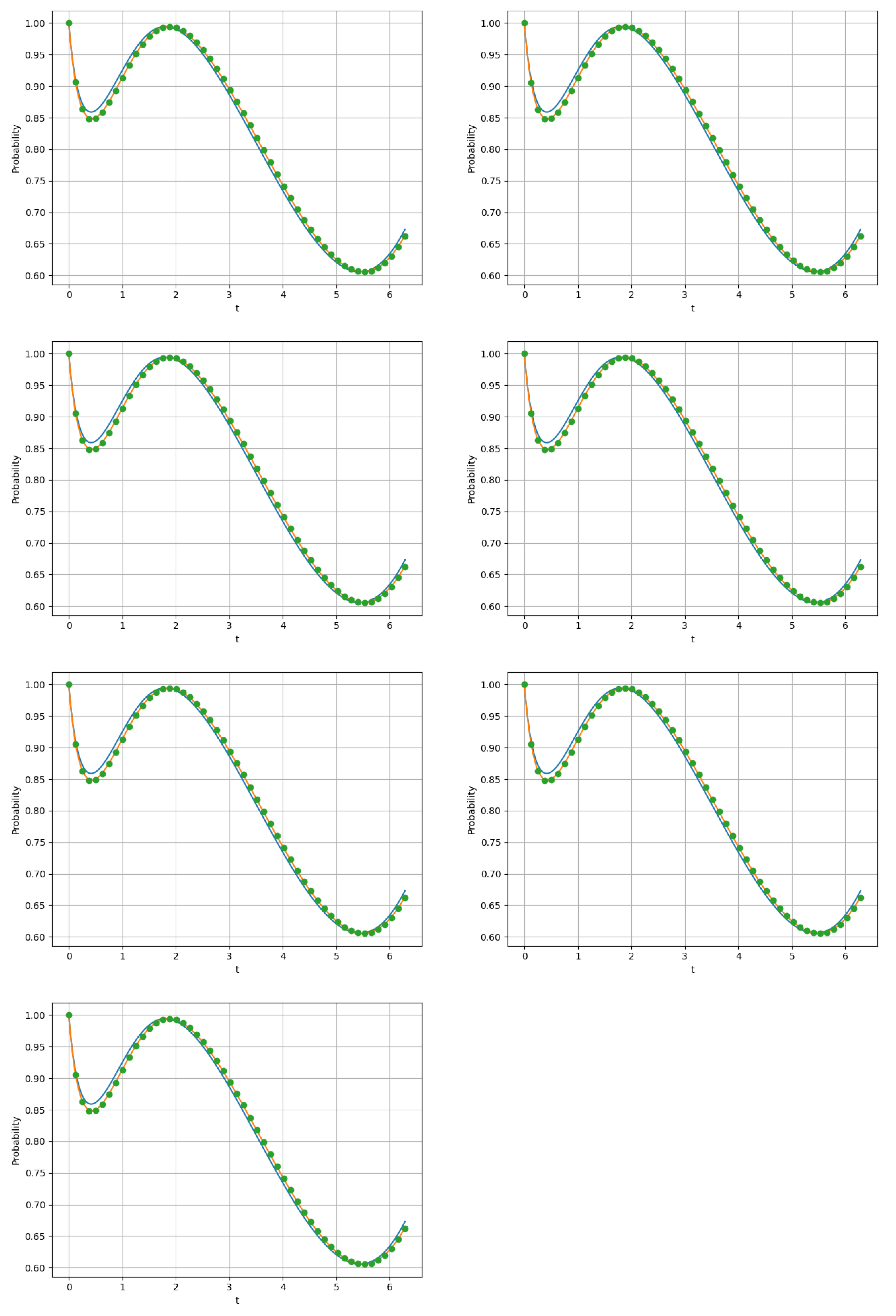
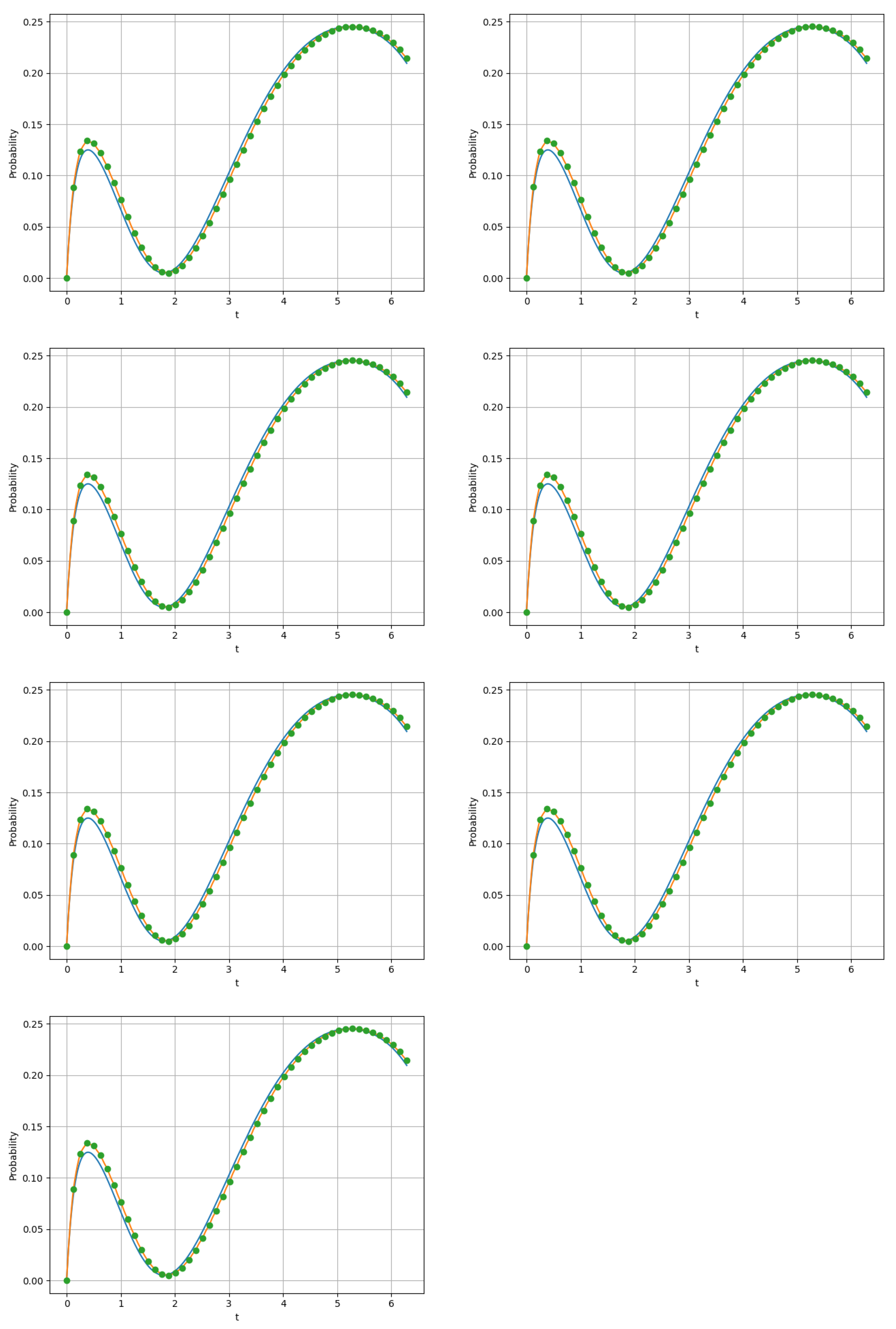
In the figures below (see Figure 2 and Figure 3), one can see the solution (blue lines) for the initial conditions X ( 0 ) = X ¯ ( 0 ) = 0 using the Runge–Kutta method and the intensity matrix A ( t ) , solution (yellow lines) using the Runge–Kutta method and the piecewise constant matrix, the solution (green dots) using matrix multiplication.
From the Table 1, it can be seen that there is no sense in increasing the value of n indefinitely, since the most significant part of the approximation error is due to the substitution of the piecewise constant matrix instead of the original one. In general, to reduce the approximation error, one should increase both n and N.

5.3. Example 3

The major contribution in the approximation error is made when the initial matrix A ( t ) is changed to the piecewise constant matrix under condition that A ( t ) changes rapidly due to the large value of ε . In this example will be made the same computation as in second example, except for the fact that here the intensity matrix A ( t ) does not depend on t. This substantially reduces the approximation error: in the right part of (16), ε becomes equal to 0 (since discretization is no longer needed) and the only error left is due to (15).
Consider the birth–death process with 31 states, with arrival and death intensities equal to λ ( t ) = 1 , μ ( t ) = 5 , respectively. Break the interval [ 0 , 2 π ] interval into N intervals of equal length. The approximation error is bounded by
p ( T ) p ¯ ( T ) ( 1 + G ) N 1 .
The Table 2 demonstrates its quality for N = 40 .
As can be seen from the second column, the solutions by the Runge–Kutta method and the matrix method are identical; the approximation error, shown in the fourth column, significantly overestimates the difference.
Note that in the considered context, i.e., when A ( t ) does not depend on t, the increase of N makes the situation worse and increases the approximation error. For example, for N = 1 and n = 10 , we have that p ( T ) p ¯ ( T ) 0.00004 .
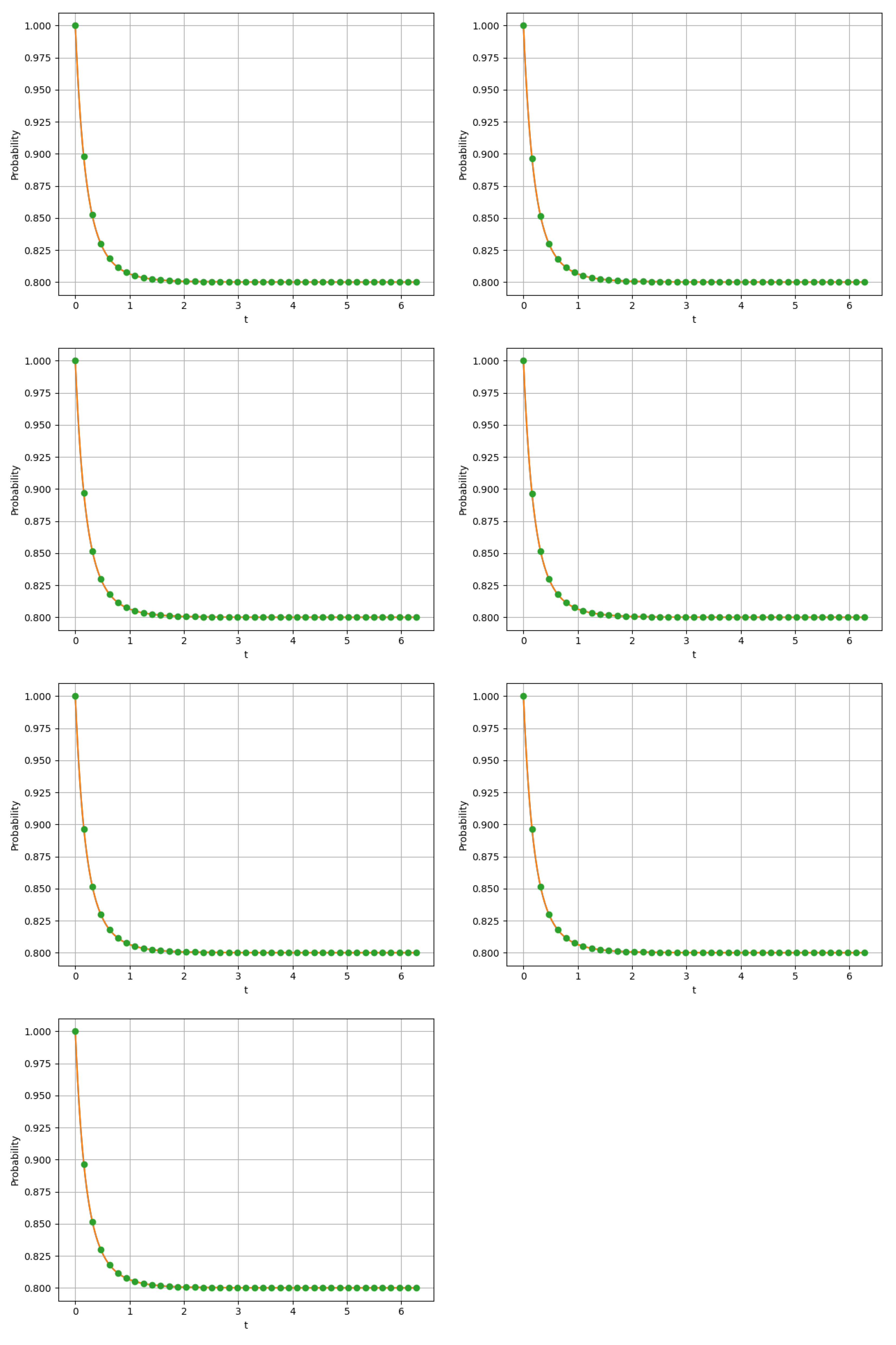
In the figures below (see Figure 4 and Figure 5), one can see the solution (yellow lines) for the initial conditions X ( 0 ) = X ¯ ( 0 ) = 0 using the Runge–Kutta method and the intensity matrix A ( t ) (one can see that the solution for the system with the piecewise constant matrix will be the same), the solution (green dots) using matrix multiplication.

6. Conclusions

In this paper, the novel variation of the well-known method for the computation of the transient distribution of the finite state time-varying Markov chains has been proposed. Its main advantage is that, if the two chains start in the same state, then within a finite horizon one can bound the difference between their probability distributions. The generalization to the countable state space is the direction for further research and it seems to be feasible since the truncation bounds are available for inhomogeneous CTMC with countable state space.

Author Contributions

Conceptualization, supervision, A.Z.; methodology, Y.S.; software, validation, visualization I.U.; investigation, writing, R.R., Y.S. and A.Z. All authors have read and agreed to the published version of the manuscript.

Funding

The research was supported by the Ministry of Science and Higher Education of the Russian Federation, project No. 075-15-2020-799.

Data Availability Statement

Not applicable.

Conflicts of Interest

The authors declare no conflict of interest.

References

  1. Schwarz, J.A.; Selinka, G.; Stolletz, R. Performance analysis of time-dependent queueing systems: Survey and classification. Omega 2016, 63, 170–189. [Google Scholar] [CrossRef]
  2. Kwon, S.; Gautam, N. Guaranteeing performance based on time-stability for energy-efficient data centers. IIE Trans. 2016, 48, 812–825. [Google Scholar] [CrossRef]
  3. Whitt, W.; You, W. Time-Varying Robust Queueing. Oper. Res. 2019, 67, 1766–1782. [Google Scholar] [CrossRef]
  4. Zeifman, A.; Satin, Y.; Kovalev, I.; Razumchik, R.; Korolev, V. Facilitating Numerical Solutions of Inhomogeneous Continuous Time Markov Chains Using Ergodicity Bounds Obtained with Logarithmic Norm Method. Mathematics 2021, 9, 42. [Google Scholar] [CrossRef]
  5. Vishnevsky, V.; Vytovtov, K.; Barabanova, E.; Semenova, O. Analysis of a MAP/M/1/N queue with periodic and non-periodic piecewise constant input rate. Mathematics 2022, 10, 1684. [Google Scholar] [CrossRef]
  6. Barabanova, E.A.; Vishnevsky, V.M.; Vytovtov, K.A.; Semenova, O.V. Methods of analysis of information-measuring system performance under fault conditions. Phys. Bases Instrum. 2022, 11, 49–59. [Google Scholar]
  7. Green, L.; Kolesar, P. The pointwise stationary approximation for queues with nonstationary arrivals. Manag. Sci. 1991, 37, 84–97. [Google Scholar] [CrossRef]
  8. Reibman, A.; Trivedi, K. Numerical transient analysis of markov models. Comput. Oper. Res. 1988, 15, 19–36. [Google Scholar] [CrossRef]
  9. Van Dijk, N.M.; van Brummelen, S.P.J.; Boucherie, R.J. Uniformization: Basics, extensions and applications. Perform. Eval. 2018, 118, 8–32. [Google Scholar] [CrossRef]
  10. Di Crescenzo, A.; Nobile, A.G. Diffusion approximation to a queueing system with time-dependent arrival and service rates. Queueing Syst. 1995, 19, 41–62. [Google Scholar] [CrossRef]
  11. Di Crescenzo, A.; Giorno, V.; Nobile, A.G.; Ricciardi, L.M. On the M/M/1 queue with catastrophes and its continuous approximation. Queueing Syst. 2003, 43, 329–347. [Google Scholar] [CrossRef]
  12. Arns, M.; Buchholz, P.; Panchenko, A. On the numerical analysis of inhomogeneous continuous-time Markov chains. INFORMS J. Comput. 2010, 22, 416–432. [Google Scholar] [CrossRef]
  13. Taaffe, M.R.; Ong, K.L. Approximating Nonstationary Ph(t)/M(t)/s/c queueing systems. Ann. Oper. Res. 1987, 8, 103–116. [Google Scholar] [CrossRef]
  14. Clark, G.M. Use of Polya distributions in approximate solutions to nonstationary M/M/s queues. Commun. ACM 1981, 24, 206–217. [Google Scholar] [CrossRef]
  15. Massey, W.; Pender, J. Gaussian skewness approximation for dynamic rate multiserver queues with abandonment. Queueing Syst. 2013, 75, 243–277. [Google Scholar] [CrossRef]
  16. Burak, M.R.; Korytkowski, P. Inhomogeneous CTMC Birth-and-Death Models Solved by Uniformization with Steady-State Detection. ACM Trans. Model. Comput. Simul. 2020, 30, 1–18. [Google Scholar] [CrossRef]
  17. Faddy, M. A note on the general time-dependent stochastic compartmental model. Biometrics 1976, 32, 443–448. [Google Scholar] [CrossRef]
  18. Zeifman, A.; Korolev, V.; Satin, Y. Two Approaches to the Construction of Perturbation Bounds for Continuous-Time Markov Chains. Mathematics 2020, 8, 253. [Google Scholar] [CrossRef]
  19. Daleckii, J.L.; Krein, M.G. Stability of solutions of differential equations in Banach space. Am. Math. Soc. 2002, 43, 1024–1102. [Google Scholar]
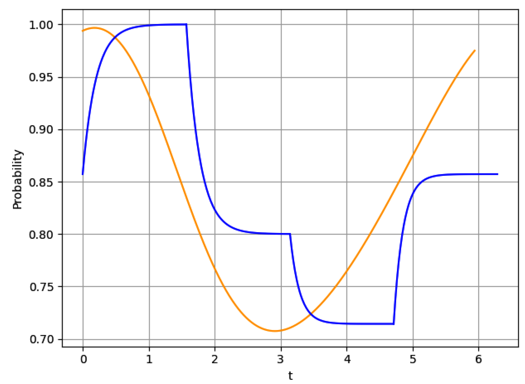
Figure 1. Example 1. Behavior of p 0 ( t ) : blue line—exact solution, orange line—approximate solution.
Mathematics 11 04265 g001
Figure 2. Behavior of p 0 ( t ) for various values of n.
Mathematics 11 04265 g002
Figure 3. Behavior of p 1 ( t ) for various values of n.
Mathematics 11 04265 g003
Figure 4. Behavior of p 0 ( t ) for various values of n. The initial conditions are X ( 0 ) = X ¯ ( 0 ) = 0 .
Mathematics 11 04265 g004
Figure 5. Behavior of p 1 ( t ) for various values of n. The initial conditions are X ( 0 ) = X ¯ ( 0 ) = 0 .
Mathematics 11 04265 g005
Table 1. Example 2: approximation error for various values of n.
n p ( 2 π ) p ¯ ( 2 π ) G ( 1 + G ) N 1 ( 1 + G ) N 1 + 0.136
40.02144931153977276≤0.41≤28,903,845≤28,903,846
50.02137755886467509≤0.13≤450≤451
60.02138771528374614≤0.035≤5≤6
70.021386393661019132≤0.009≤0.57≤0.706
80.021386550440098923≤0.002≤0.11≤0.245
90.021386533366325292≤0.0004≤0.021≤0.157
100.02138653508102207≤0.00007≤0.004≤0.14
Table 2. Example 3: approximation error for various values of n.
n p ( 2 π ) p ¯ ( 2 π ) G ( 1 + G ) N 1
4≤4 × 10 10 ≤0.28321,333
5≤2 × 10 11 ≤0.0931
6≤7 × 10 13 ≤0.022 1.34
7≤3 × 10 14 ≤0.005 0.23
8≤9.99 × e 14 ≤0.002 0.09
9≤9.99 × e 14 ≤0.0002 0.009
10≤9.99 × e 14 ≤0.00004 0.002
Disclaimer/Publisher’s Note: The statements, opinions and data contained in all publications are solely those of the individual author(s) and contributor(s) and not of MDPI and/or the editor(s). MDPI and/or the editor(s) disclaim responsibility for any injury to people or property resulting from any ideas, methods, instructions or products referred to in the content.