Mathematical Modeling Reveals Mechanisms of Cancer-Immune Interactions Underlying Hepatocellular Carcinoma Development

Abstract

Understanding the relationship between hepatocellular carcinoma (HCC) and immunity is crucial for HCC immunotherapy. However, the existing research has solely focused on a novel population of primary tumor-induced non-leukocytes called Ter-cells and their circulating components in distant organs, neglecting the examination of immunity’s impact on cancer. In order to thoroughly examine the dynamics of Ter cells, HCC, and the known regulatory elements in the immunological milieu, we used a mathematical model in the form of a system of differential equations in this work. According to simulation studies, tumor cells cannot be completely eliminated by either the effective killing of HCC by cytotoxic T lymphocytes (CTL) or the inhibition of tumor cell proliferation. Nonetheless, continuous CTL activation and TGF-$\beta$-induced differentiation of CTL facilitated a transition from a high steady-state of HCC quantity to an unstable state, followed by a low state of HCC quantity, aligning with the three phases of the cancer immunoediting concept (escape, equilibrium, and elimination). Our survival study revealed that the ratio of CTL proliferation to CTL killing and relative TGF-$\beta$-induced differentiation of CTL have a significant impact on cancer-free survival. Sensitivity and bifurcation analysis of these parameters demonstrated that the rate of CTL proliferation, as well as the number of HCCs when the production rate reaches half of one, strongly affects the number of HCCs. Our findings highlight the critical role of immune system activation in cancer therapy and its potential impact on HCC treatment.

1. Introduction

The second greatest cause of cancer-related deaths globally is hepatocellular carcinoma (HCC) [1]. It is characterized by high lethality, a significant risk of intra- and extrahepatic metastasis, and post-surgical recurrence [2]. Extensive efforts have been devoted to understanding the pathophysiology and treatment of HCC due to its significance. Previous clinical and biological experimental data have linked various genetic events, such as the inactivation of the tumor suppressor p53, mutations in the $\beta$-catenin and TGF-$\beta$ pathway genes, and overexpression of ErbB receptor family members (ERBB1, ERBB3, etc.) and the MET receptor, to HCC development [3,4,5]. Therapeutic interventions targeting these genes and their associated gene expressions have shown promise in treating cancer.

From an immunotherapy perspective, tumor development undergoes three distinct phases known as the cancer immunoediting process, namely “elimination”, “equilibrium”, and “escape” [6,7,8]. The cancer immunoediting concept aims to integrate the dual effect of the immune system on advanced tumor formation. Notably, the immune system not only suppresses tumor formation by eliminating cancer cells but also facilitates the survival of specific cancer cells by establishing conditions within the tumor microenvironment [9]. This concept provides a novel research perspective for cancer therapy.

Significant progress has been made in the field of HCC immunotherapy through in-depth studies. For instance, spontaneous T cell responses against numerous tumor antigens, including alpha-fetoprotein (AFP), glypican-3 (GPC3), NY-ESO-1, SSX-2, MAGE-A10, and p53, have been detected in HCC patients [10,11,12]. Overactive signaling of TGF-$\beta$ contributes to immunosuppression [3]. However, the failure of the immune system to respond appropriately is likely due to multiple immune-suppressive mechanisms regulated by the tumor itself [13]. Increased populations of immunosuppressive myeloid and lymphoid cells, suppression of natural killer (NK) cells, and up-regulation of immune checkpoint pathways have been reported to impair the normal function of cellular immunity [14,15,16]. Notably, the number of T regulatory cells (Tregs) rises in both the peripheral blood and the tumor, and Treg accumulation is often associated with poor prognosis [17,18].

Hepatocellular carcinoma can be treated in a variety of ways, including chemotherapy, immunotherapy, targeted therapy, immune checkpoint inhibitors, gene therapy, radiotherapy, and combination therapy [19,20,21,22,23]. A population of tumor-inducible erythroblast-like cells (Ter-cells) that are enriched in the spleen of HCC-bearing mice were recently discovered by Han et al. [24]. TGF-$\beta$-activated Ter-cells promote tumor progression by secreting the neurotrophic factor artemin into the bloodstream. And scientists continue to explore just how they impact HCC. The treatment of dynamic diseases will be aided by a full understanding of the related mechanisms of action, which will provide insight into biological processes, which is in contrast to other techniques for spotting the onset of cancer, like the study of High throughput screening data analysis, single cell analysis, microarray datasets, and RNA seq data.

Discovering the mechanisms underlying cancer treatment has been substantially facilitated by dynamic modeling, which is regarded as an efficient mathematical tool for analyzing dynamic interactions [25,26]. A pharmacokinetic-pharmacodynamic model was utilized to relate drug exposure to tumor growth inhibition (TGI) and time to tumor progression (TTP) via sVEGFR2 kinetics using the angiogenic biomarker sunitinib [27]. As a reference medication for the treatment of advanced hepatocellular carcinoma (HCC), sorafenib inhibits the RAF-MEK-ERK cascade response in HCC cells. Based on prior research demonstrating that sorafenib is a potent inhibitor of this cascade in HCC cells, the regulatory mechanisms were investigated using mathematical modeling and ordinary differential equations [28]. Additionally, mathematical models [29] based on the dynamic biological interactions between the immune system and the tumor simulate the application of a combined regimen of immune checkpoint inhibitors (ICIs) and radiation therapy (RT) to clinical experimental studies of patients with HCC. Another mathematical model [30] that quantifies the immunostimulatory and immunosuppressive effects of radiation therapy and simulates the effects of immune checkpoint inhibitors and radiation therapy is also based on the predator-prey model. Combining chemotherapy and immunotherapy, a six-dimensional system in which the cancer cells have a logistic growth type has been established in [31] that can be can provide the dynamic interactions between the tumor cells, immune system, and drug-response systems, a non-autonomous ODE system can help to gain insight into the cooperative interaction between anti-TGF-$\beta$ and vaccine treatments [32] by taking into account the three variables tumor, CTL, and TGF-$\beta$.

Each biological connection in this complex web may be represented in various ways. However, for the sake of simplifying the model and facilitating theoretical analysis in this article, our primary objective is to quantitatively analyze the dynamics of HCC, Ter cells, and HCC-derived circulating factors in the immune environment through dynamic modeling. This analysis is built upon existing discoveries in the field. In the complicated tumor microenvironment, interactions between various cells and cytokines are frequent occurrences. The findings we have reached here solely emphasize the role of cytotoxic T lymphocytes (CTLs) in the development of hepatocellular carcinoma (HCC) and do not delve into the functions of other cell types. Specifically, we aim to address the relationship among cytotoxic T cell (CTL), HCC, and Ter cells together with the circulating factors serum artemin and serum TGF-$\beta$, and realize the goal of controlling and curing cancer through affecting the five research objects and their interactions to gain insights into the progression of HCC and the potential impact of immunotherapy approaches. We also understand how variations in baseline settings and interactions between individuals impact survival rates. Standard treatments for HCC, including pharmaceutical therapy, chemotherapy, and surgical resection, have intrinsic limitations. Our research emphasizes the critical function of cellular immunity in the treatment of HCC and demonstrates that activating CTL is the most efficient way to get rid of HCC, offering a promising avenue for the development of targeted immunotherapies against this aggressive cancer.

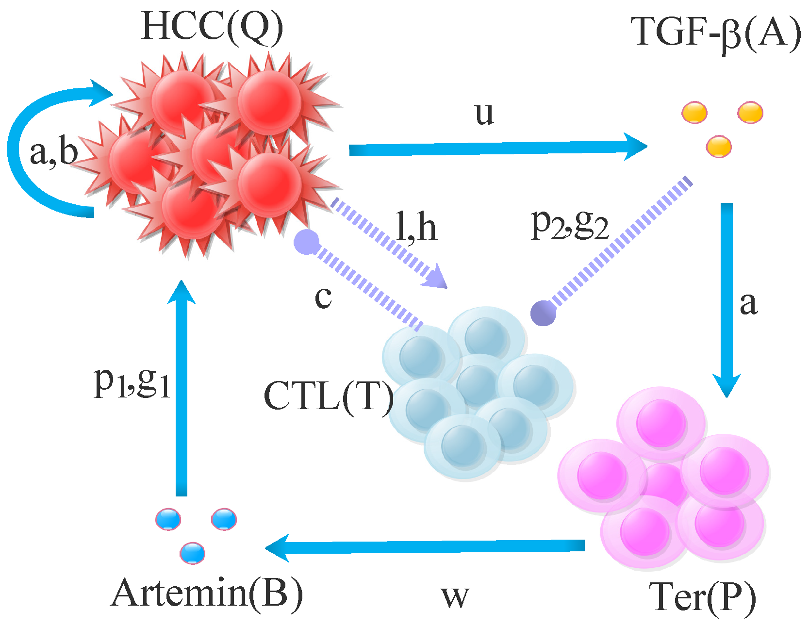
2. Mathematical Modeling

During HCC development and progression, new erythroid-like cells (Ter cells) encourage tumor growth by secreting the neurotrophic factor Artemin. Additionally, Ter cell generation is significantly influenced by TGF-$\beta$ activation [24]. Hepatocellular carcinoma cells that express TGF-$\beta$ encourage the development of Ter cells, whereas Ter cells that produce Artemin protein encourage the growth of tumors [24]. Inflammation, fibrogenesis, and immunomodulation in the HCC microenvironment are all significantly influenced by dysregulated signaling in the TGF-$\beta$ pathway. Effector T cells, which have been discovered to have a specialized immunological role against hepatocellular carcinoma cells, have been shown to be transformed by TGF-$\beta$ into regulatory T cells, which have the capacity to stifle immunity and the inflammatory response [33]. It makes sense to speculate that TGF-$\beta$ inhibits the generation of cytotoxic T cells, and at the same time, we speculate that hepatocellular carcinoma cells encourage the proliferation and aggregation of cytotoxic T cells, that cytotoxic T cells promote hepatocellular carcinoma cells’ apoptosis, and that hepatocellular carcinoma cells have the ability to self-proliferate. Since serum can, be obtained in other ways besides injection, it can be believed that both sera are continuously produced. By integrating them into the current regulatory network [24], we can establish plausible connections between Ter-cells, HCC, CTLs, serum TGF-$\beta$, and serum artemin (Figure 1).

We first have developed a novel set of five-variable ordinary differential equations (ODEs) based on our network model. The variables in the equations represent the counts of HCC cells, Ter cells, and CTLs, as well as the concentrations of serum TGF-$\beta$ and serum artemin, denoted as Q, P, T, A, and B, with respect to time $\tau$ respectively.

$$\begin{array}{c}\hfill \left\{\begin{array}{c}\frac{dQ}{d\tau }=\underset{\mathrm{HCC}\mathrm{proliferation}}{\underbrace{aQ(1-bQ)}}+\underset{\mathrm{artemin}\mathrm{induced}\mathrm{proliferation}}{\underbrace{\frac{p_{1}BQ}{g_1+B}}}-\underset{\mathrm{HCC}\mathrm{killed}\mathrm{by}\mathrm{CD}8+\mathrm{T}\mathrm{cell}}{\underbrace{cTQ}},\hfill \\ \frac{dP}{d\tau }=\underset{\mathrm{promotion}\mathrm{by}\mathrm{TGF}\text{-}\beta }{\underbrace{\alpha A}}-\underset{\mathrm{death}}{\underbrace{rP}},\hfill \\ \frac{dT}{d\tau }=\underset{\mathrm{activation}\mathrm{by}\mathrm{HCC}}{\underbrace{\frac{lQT}{h+Q}}}-\underset{\mathrm{inhibition}\mathrm{by}\mathrm{TGF}\text{-}\beta }{\underbrace{\frac{p_{2}AT}{g_2+A}}}-\underset{\mathrm{death}}{\underbrace{eT}},\hfill \\ \frac{dA}{d\tau }=\underset{\mathrm{activation}\mathrm{by}\mathrm{HCC}}{\underbrace{uQ}}-\underset{\mathrm{degradation}}{\underbrace{vA}}+\underset{\mathrm{production}}{\underbrace{d_1}},\hfill \\ \frac{dB}{d\tau }=\underset{\mathrm{activation}\mathrm{by}\mathrm{Ter}}{\underbrace{wP}}-\underset{\mathrm{degradation}}{\underbrace{kB}}+\underset{\mathrm{production}}{\underbrace{d_2}}.\hfill \end{array}\right.\end{array}$$

(1)

To simplify the analysis and reduce the number of parameters, we introduce constants $A_0$ and $B_0$. Furthermore, we non-dimensionalize the model using the following substitutions:

$$\begin{array}{c}X=bQ,Y=bP,Z=bT,L=\frac{A}{100A_0},M=\frac{B}{B_0},t=e\tau .\end{array}$$

where $\frac{1}{b},e,A_0,B_0$ represent tumor carrying capacity, death rate of CTL, initial concentration of TGF-$\beta$, initial concentration of artemin.

The simplified model takes the following form:

$$\begin{array}{c}\hfill \left\{\begin{array}{c}\frac{dX}{dt}=k_{1}X(1-X)+\frac{k_{2}XM}{k_3+M}-k_{4}XZ,\hfill \\ \frac{dY}{dt}=k_{5}L-k_{6}Y,\hfill \\ \frac{dZ}{dt}=\frac{k_{7}XZ}{k_8+X}-\frac{k_{9}LZ}{k_{10}+L}-Z,\hfill \\ \frac{dL}{dt}=k_{11}X-k_{12}L+k_{13},\hfill \\ \frac{dM}{dt}=k_{14}Y-k_{15}M+k_{16}.\hfill \end{array}\right.\end{array}$$

(2)

where

$$\begin{array}{cc}\hfill & k_1=\frac{a}{e},k_2=\frac{p_1}{e},k_3=\frac{g_1}{B_0},k_4=\frac{c}{be},k_5=\frac{100A_{0}b\alpha }{e},k_6=\frac{r}{e},\hfill \\ \hfill & k_7=\frac{l}{e},k_8=bh,k_9=\frac{p_2}{e},k_{10}=\frac{g_2}{100A_0},k_{11}=\frac{u}{100A_{0}be},\hfill \\ \hfill & k_{12}=\frac{v}{e},k_{13}=\frac{d_1}{100A_{0}e},k_{14}=\frac{w}{B_{0}be},k_{15}=\frac{k}{e},k_{16}=\frac{d_2}{B_{0}e}.\hfill \end{array}$$

(3)

All parameters and their biological meaning are listed in

Table A1. The Optimal Parameters.

Symbol	Units	Biological Meanings
a	${\mathrm{day}}^{-1}$	Tumor growth rate
b	${\mathrm{cell}}^{-1}$	$\frac{1}{b}=$ tumor carrying capacity
c	${\mathrm{cell}}^{-1}{\mathrm{day}}^{-1}$	Killing rate of T cells on tumor cells
$p_1$	${\mathrm{day}}^{-1}$	The maximum rate that artemin activates tumor cell
$g_1$	$\mathrm{ng}·{\mathrm{mL}}^{-1}$	Steepness coefficient of the HCC proliferation curve
$\alpha$	$\frac{\mathrm{cells}·\mathrm{mL}}{\mathrm{ng}·\mathrm{day}}$	Rate at which Ter cells are generated by TGF-$\beta$
r	${\mathrm{day}}^{-1}$	Death rate of Ter cells
l	${\mathrm{day}}^{-1}$	The proliferation rate of tumor-specific CTL
h	$\mathrm{cell}$	Number of HCC when the producing rate reaches half of l
$p_2$	${\mathrm{day}}^{-1}$	TGF-$\beta$ related differentiation of CTL
$g_2$	$\mathrm{ng}·{\mathrm{mL}}^{-1}$	Coefficient of CTL differentiation
e	${\mathrm{day}}^{-1}$	Death rate of CTL
u	$\frac{\mathrm{ng}}{\mathrm{mL}·\mathrm{cells}·\mathrm{day}}$	Producing rate of TGF-$\beta$ by HCC
v	${\mathrm{day}}^{-1}$	Death rate of TGF-$\beta$
w	$\frac{\mathrm{ng}}{\mathrm{mL}·\mathrm{cells}·\mathrm{day}}$	Producing rate of artemin by Ter cell
k	${\mathrm{day}}^{-1}$	Death rate of artemin
$A_0$	$\mathrm{ng}·{\mathrm{mL}}^{-1}$	Initial concentration of TGF-$\beta$
$B_0$	$\mathrm{ng}·{\mathrm{mL}}^{-1}$	Initial Concentration artemin
$d_1$	$\mathrm{ng}·{\mathrm{mL}}^{-1}·{\mathrm{day}}^{-1}$	Production rate of TGF-$\beta$
$d_2$	$\mathrm{ng}·{\mathrm{mL}}^{-1}·{\mathrm{day}}^{-1}$	Production rate of artemin

. And Every parameter function is bounded and nonnegative. All subsequent analyses are conducted based on the dimensionless model (Equation (2)). Next we perform a new theoretical analysis regarding the five-dimensional system (2) we have established.

3. Theoretical Properties of the Model

3.1. Nonnegativity of Solutions

The dimensionless model exhibits the following fundamental properties, as stated by

Theorem 1. 

For any nonnegative initial value ${\varphi }_0=(X\left(0\right),Y\left(0\right),Z\left(0\right),L\left(0\right),M\left(0\right))$, each solution $\varphi \left(t\right)=\left(X\right(t),Y(t),Z(t),L(t),M(t\left)\right)$ of system (2) remains nonnegative through ${\varphi }_0$ for all $t\ge 0$.

Proof. 

Let the initial values ${\varphi }_0$ of the variables of the system (2) be nonnegative,

$$\begin{array}{c}\frac{dX}{dt}{|}_{X=0}=0,\frac{dY}{dt}{|}_{Y=0}=k_{5}L\ge 0,\frac{dZ}{dt}{|}_{Z=0}=0,\\ \frac{dL}{dt}{|}_{L=0}=k_{11}X+k_{13}\ge 0,\frac{dM}{dt}{|}_{M=0}=k_{14}Y+k_{16}\ge 0.\end{array}$$

It is feasible to draw the conclusion that based on the comparison principle and the dependence on the initial value. □

Theorem 1 indicates that if the system is initiated from an interior point of $R_5^{+}$, then the five variables remain non-negative, making the region $R_5^{+}$ an invariant set. Furthermore, we can assert that the invariant set is constrained within a more specific region, specifically a non-negative invariant region.

3.2. Nonnegative Invariant

Theorem 2. 

For any initial value ${\varphi }_0=(X\left(0\right),Y\left(0\right),Z\left(0\right),L\left(0\right),M\left(0\right))\in \Gamma$, system (2) has a unique nonnegative bounded solution $\varphi \left(t\right)=\left(X\right(t),Y(t),Z(t),L(t),M(t\left)\right)$ through ${\varphi }_0$ for all $t\ge 0$, where

$$\begin{array}{c}\Gamma =[0,1]\times [0,\frac{k_5{k}_{11}+k_5{k}_{13}}{k_6{k}_{12}}]\times [0,+\infty )\times [0,\frac{k_{11}+k_{13}}{k_{12}}]\times [0,\frac{k_5{k}_{14}{k}_{11}+k_5{k}_{13}{k}_{14}+k_6{k}_{12}{k}_{16}}{k_6{k}_{12}{k}_{15}}].\end{array}$$

is nonnegative invariant set.

Proof. 

Firstly we assume that the initial values of the variables ${\varphi }_0$ are non-negative, and we can give the following notation: $\varphi \left(t\right)$ is a solution of the system (2), and $G\left(\varphi \right)$ is the vector field described by (2) with $\varphi \in \Gamma$. The third equation of (2) shows that when t is close to 0,

$$-(k_9+1)Z\le \frac{dZ}{dt}=\frac{k_{7}XZ}{k_8+X}-\frac{k_{9}LZ}{k_{10}+L}-Z\le (k_7-1)Z$$

which indicates that $Z\left(t\right)\ge 0$ using the standard comparison theory for differential inequalities. Let $\overline{Z}=max\left(Z\left(t\right)\right)$, so $0<\overline{Z}<+\infty$,

$$(k_1-k_4\overline{Z})X-k_1{X}^2\le \frac{dX}{dt}=k_{1}X(1-X)+\frac{k_{2}XM}{k_3+M}-k_{4}XZ\le (k_1+k_2)X-k_1{X}^2.$$

By employing the comparison theory for differential inequalities, we derive the inequalities $H_2\left(t\right)\le X\left(t\right)\le H_1\left(t\right)$, where $H_2\left(0\right)=X\left(0\right)=H_1\left(0\right),H_2\left(t\right)\ge 0,H_1\left(t\right)$ monotonically approaches $1+\frac{k_2}{k_1}$. Considering the biological meaning, where X(t) represents the dimensionless tumor size, it can be concluded that $X\left(t\right)\le 1$. In biological terms, this means that the dimensionless tumor size, X, should remain below the relative maximum tumor carrying capacity −1. Similarly, we can establish upper and lower bounds for the variables Y, L, and M. These properties persist as long as all variables remain non-negative. Consequently, we define the domain $\Gamma$ as the region from which the system (2) originates and from which it will never escape.

Since $G\left(\varphi \right)$ is a continuously differentiable function, we can infer that $G\left(\varphi \right)$ is locally Lipschitz continuous, then we can conclude that there exists a unique solution $\varphi \left(t\right)\in \Gamma$ of the system (2). □

Corollary 1. 

If $k_7\le 1$, the invariant set of the system (2) becomes

$$\begin{array}{c}{\Gamma }_0=[0,1]\times [0,\frac{k_5{k}_{11}+k_5{k}_{13}}{k_6{k}_{12}}]\times [0,ϵ)\times [0,\frac{k_{11}+k_{13}}{k_{12}}]\times [0,\frac{k_5{k}_{14}{k}_{11}+k_5{k}_{13}{k}_{14}+k_6{k}_{12}{k}_{16}}{k_6{k}_{12}{k}_{15}}],\\ \forall 0<ϵ\le 1.\end{array}$$

Corollary 1 indicates that the relative counts of CTLs (Z)-the third variable in the equation become very small and positive if the relative proliferation rate of tumor-specific CTL($k_7$) is less than 1.

3.3. Existence and Local Stability of Equilibrium Points

Our objective is to identify the equilibrium points of the ordinary differential equations (ODEs) that correspond to the biological process of cancer immunity. To assess the local stability of these equilibrium points, we examine the corresponding eigenvalues of the Jacobian Matrix.

Theorem 3. 

There always exists an unstable equilibrium solution

$$E_0=(0,\frac{k_5{k}_{13}}{k_6{k}_{12}},0,\frac{k_{13}}{k_{12}},\frac{k_5{k}_{13}{k}_{14}+k_6{k}_{12}{k}_{16}}{k_6{k}_{12}{k}_{15}}),$$

for the system (2) in nonnegative invariant set Γ.

Proof. 

Finding an expression for the equilibrium solution $E_0$ is obvious when looking for a cancer-free equilibrium solution where X = 0. Furthermore, the Jacobian Matrix

$$\begin{array}{cc}\hfill J& =\left[\begin{array}{ccccc}{k}_1+\frac{k_2(k_5{k}_{13}{k}_{14}+k_6{k}_{12}{k}_{16})}{k_3{k}_6{k}_{12}{k}_{15}+k_5{k}_{13}{k}_{14}+k_6{k}_{12}{k}_{16}}& 0& 0& 0& 0\\ 0& -k_6& 0& k_5& 0\\ 0& 0& \frac{-k_9{k}_{13}}{k_{10}{k}_{12}+k_{13}}-1& 0& 0\\ k_{11}& 0& 0& -k_{12}& 0\\ 0& k_{14}& 0& 0& -k_{15}\end{array}\right].\hfill \end{array}$$

It is evident that one of the Jacobi matrix’s eigenvalues is

$$k_1+\frac{k_2(k_5{k}_{13}{k}_{14}+k_6{k}_{12}{k}_{16})}{k_3{k}_6{k}_{12}{k}_{15}+k_5{k}_{13}{k}_{14}+k_6{k}_{12}{k}_{16}}>0.$$

Thus the equilibrium solution $E_0$ has been proven to be unstable. □

One notable equilibrium point in the model represents a cancer-free state ($E_0$), which is unstable but indicates a possible consequence of HCC evolution.

Another state, immune escape ($E_{*}=(X_{*},Y_{*},0,L_{*},M_{*})$), implies the absence of tumor-specific cellular immunity, leading to tumorigenesis. However, the equilibrium solution for this state does not exist. Furthermore, we have demonstrated the existence of an additional equilibrium point under certain conditions. Firstly, let

$$\begin{array}{c}\overline{\mathcal{A}}=k_{10}(k_7-1),\overline{\mathcal{B}}=k_8{k}_{10},\overline{\mathcal{C}}=k_8(k_9+1),\overline{\mathcal{D}}=k_9+1-k_7,\\ \mathcal{A}=k_{11}\overline{\mathcal{D}},\mathcal{B}=k_{11}\overline{\mathcal{C}}+k_{13}\overline{\mathcal{D}}-k_{12}\overline{\mathcal{A}},\mathcal{C}=k_{13}\overline{\mathcal{C}}+k_{12}\overline{\mathcal{B}},\Delta ={\mathcal{B}}^2-4\mathcal{A}\mathcal{C},\\ a_1=-k_1{X}_1,a_3=-k_4,a_5=\frac{k_2{k}_3{X}_1}{{(k_3+M_1)}^2},b_2=-k_6,b_4=-k_5,\\ c_1=\frac{k_7{k}_8{Z}_1}{{(k_8+X_1)}^2},c_4=-\frac{k_9{k}_{10}{Z}_1}{{(k_{10}+L_1)}^2},d_1=k_{11},d_4=-k_{12},e_2=k_{14},e_5=-k_{15},\\ R_2=a_5{b}_4{e}_2,P_2=b_2{e}_5,P_1=b_2+e_5,Q_1=a_1+d_4,Q_2=a_1{d}_4-a_3{c}_1,\\ Q_3=a_3{c}_4{d}_1,N_1=P_1+Q_1,N_2=Q_2+P_2+P_1{Q}_1,\\ N_3=Q_3+P_2{Q}_1+P_1{Q}_2,N_4=P_2{Q}_2+P_1{Q}_3-R_2,N_5=P_2{Q}_3.\end{array}$$

Assume the following conditions:

$\left(H_1\right):k_9+1-k_7<0,k_7-1<0,\Delta >0,2\mathcal{A}+\mathcal{B}\ge 0,\mathcal{A}+\mathcal{B}+\mathcal{C}\ge 0,$

$\left(H_2\right):k_9+1-k_7<0,k_7-1<0,\Delta >0,2\mathcal{A}+\mathcal{B}\le 0$,

$\left(H_3\right):k_9+1-k_7>0,k_7-1>0,\Delta \ge 0,2\mathcal{A}+\mathcal{B}\ge 0,\mathcal{A}+\mathcal{B}+\mathcal{C}\ge 0,\mathcal{B}<0,$

$\left(H_4\right)$: All the solutions have negative real parts for the equation

$${\lambda }^5-N_1{\lambda }^4+N_2{\lambda }^3-N_3{\lambda }^2+N_4\lambda -N_5=0.$$

(4)

Theorem 4. 

System (2) possesses another type of positive equilibrium point, denoted as  $E_1=(X_1,Y_1,Z_1,L_1,M_1)$, where $X_1$ satisfies the equation

$$\mathcal{A}{X}^2+\mathcal{B}X+\mathcal{C}=0.$$

(5)

The existence of non-negative real equilibrium points is determined by the solution to this equation. Additionally, the values of $Y_1,Z_1,L_1,$ and $M_1$ are determined by specific expressions provided in the following

$$\begin{array}{c}\hfill Y_1=\frac{k_5}{k_6{k}_{12}}(k_{11}{X}_1+k_{13}),Z_1=\frac{1}{k_4}[k_1(1-X_1)+\frac{k_2{M}_1}{k_3+M_1}],\\ \hfill L_1=\frac{k_{11}{X}_1+k_{13}}{k_{12}}=\frac{k_{10}(\frac{k_7{X}_1}{k_8+X_1}-1)}{k_9-(\frac{k_7{X}_1}{k_8+X_1}-1)},M_1=\frac{k_5{k}_{14}(k_{11}{X}_1+k_{13})+k_6{k}_{12}{k}_{16}}{k_6{k}_{12}{k}_{15}}.\end{array}$$

Within the nonnegative invariant set $\Gamma$ for the system (2), we can draw the following conclusions:

(1) 

If assumption $\left(H_1\right)$ or $\left(H_2\right)$ is satisfied, the system (2) possesses an equilibrium solution of the $E_1$ type.

(2) 

If assumption $\left(H_3\right)$ is satisfied, there exist two equilibrium solutions of the $E_1$ type for the system (2). Furthermore, the equilibrium solution $E_1$ exists and is locally stable if assumption $\left(H_4\right)$ is satisfied.

Proof. 

If $(k_9+1-k_7)(k_7-1)>0,$ then $L=\frac{k_{10}(\frac{k_{7}X}{k_8+X}-1)}{k_9-(\frac{k_{7}X}{k_8+X}-1)}\ge 0.$ And for equation

$$\frac{k_{11}X+k_{13}}{k_{12}}=\frac{k_{10}(\frac{k_{7}X}{k_8+X}-1)}{k_9-(\frac{k_{7}X}{k_8+X}-1)},$$

(6)

if

$$\Delta \ge 0,\frac{\mathcal{C}}{\mathcal{A}}<0,$$

then Equation (6) exists one positive solution, and if

$$\Delta \ge 0,\frac{\mathcal{C}}{\mathcal{A}}>0,-\frac{\mathcal{B}}{\mathcal{A}}>0,$$

then Equation (6) exist two positive solutions, and the presence interval of these positive solutions of Equation (6) are given in the [0, 1], in consequence, we can assume conditions $\left(H_1\right)-\left(H_3\right)$, there exists equilibrium solution $E_1$ for the Equation (5). Furthermore, the Jacobian Matrix

$$\begin{array}{cc}\hfill J& ={\left[\begin{array}{ccccc}{k}_1-2k_{1}X-k_{4}Z+\frac{k_{2}M}{k_3+M}& 0& -k_{4}X& 0& \frac{k_2{k}_{3}X}{{(k_3+M)}^2}\\ 0& -k_6& 0& k_5& 0\\ \frac{k_7{k}_{8}Z}{{(k_8+Z)}^2}& 0& \frac{k_{7}X}{k_8+X}-\frac{k_{9}L}{k_{10}+L}-1& \frac{-k_9{k}_{10}Z}{{(k_{10}+L)}^2}& 0\\ k_{11}& 0& 0& -k_{12}& 0\\ 0& k_{14}& 0& 0& -k_{15}\end{array}\right]}_{{|}_{E_1}},\hfill \\ \hfill & =\left[\begin{array}{ccccc}{a}_1& 0& a_3& 0& a_5\\ 0& b_2& 0& b_4& 0\\ c_1& 0& 0& c_4& 0\\ d_1& 0& 0& d_4& 0\\ 0& e_2& 0& 0& e_5\end{array}\right].\hfill \end{array}$$

If all the solutions of corresponding eigenequations of Equation (4) have negative real parts, then the equilibrium solution $E_1$ is locally stable, which can equal assumption $\left(H_4\right)$. □

Theorem 4 elucidates that the number of non-negative equilibrium points is contingent upon the variables defined by assumptions $\left(H_1\right)-\left(H_3\right)$. Furthermore, Corollary 2, derived from Theorem 4, states the following:

Corollary 2. 

System (2) possesses a unique equilibrium point, $E_0$, only when $k_7\le 1$ and $\Delta =0$.

Corollary 2 underscores that HCC will inevitably reach an unstable equilibrium state if $\Delta =0$ and $k_7$ is less than 1, thereby highlighting the significance of $k_7$ for subsequent discussions.

4. Numerical Results

The theoretical analysis results presented earlier demonstrate that the system (2) exhibits the potential to attain two distinct stable states under specific parameter configurations, each corresponding to a unique steady state. Consequently, in this section, we will delve into the dynamic behavior of the system (2) under various initial conditions. For our analysis and numerical simulations of the dynamical system, we employed MATLAB software due to its capabilities in numerical simulation and programming. Additionally, for bifurcation analysis, we utilized XPPAUT software, known for its effectiveness in such analyses.

4.1. Sensitivity Analysis of Parameters

Global sensitivity analysis determines how the system responds to parameter perturbations in the model. To quantify the sensitivity of input parameters on all variables in the model (2), we utilize the partial rank correlation coefficient (PRCC) [34]. We employ Latin Hypercube Sampling (LHS) to generate 5000 samples for calculating PRCC and p-values of the five variables: X (HCC), Y (Ter), Z (CTL), L (TGF-$\beta$), and M (Artemin). Figure 2 illustrates that the variable X (HCC) is most sensitive to the perturbation of parameter $k_8$ (the relative number of HCC when the producing rate reaches half of l) and $k_7$ (The relative proliferation rate of tumor-specific CTL), suggesting that controlling Z, which is activated by HCC, is effective in the short-term control of HCC. Among the 16 parameters associated with various biological processes listed in Table A1, $k_2$ exhibits a significant influence on Z (CTL).

4.2. Numerical Simulations Reveal Possible Methods of Cancer Treatment

To simulate the development of HCC in the presence of immunity, we set the initial values of the system (2) as $[0.1,0.1,0.1,0.1,0.2]$. Figure 3 depicts the trajectories in three-dimensional phase space for the system with different initial values. Eventually, they converge to the point (0.43, 0.73, 0.08) as t approaches infinity.

We conducted simulations to investigate the impact of medication on reducing the proliferation rate of HCC. Figure 4a,b indicate that inhibiting HCC proliferation in the early stage, by administering treatment at the moment of maximum HCC (t = 4.887), can temporarily alleviate tumor progression without altering the final stable state. However, if treatment is missed at the maximum moment of HCC (t = 4.887), Figure 4a–c, demonstrate a significant reduction in HCC at every moment after treatment at another time point, t = 9.774. The treatment effect at t = 9.774 is superior to that at the maximum moment of HCC (t = 4.887) in the early stage, but it does not affect the final stable state. We believe that inhibiting HCC proliferation after reaching the maximum number of cancer cells at the beginning of cancer can extend survival. However, escaping immunosurveillance leads to more aggressive proliferation. Additionally, we explore the impact of chemotherapy, specifically the direct killing of HCC cells. Figure 4d,f reveal that an increase in the relative killing rate of HCC alters the rising trend of relative HCC cell counts, resulting in a longer patient lifespan. However, the tumor relief achieved through chemotherapy is transient. In the long term, HCC cell counts eventually reach the same relatively high steady state.

We also simulate tumor resection, which corresponds to a reduction in tumor cells. It is observed that relative HCC cell counts return to pre-treatment levels at a relative time of t = 6 after “tumor resection” (Figure 4e). We assume that surgical treatment has limited efficacy in eliminating HCC due to its infinite proliferation and inefficient killing. To investigate the role of cellular immunity in autonomous anticancer mechanisms, we simulate the dynamics of HCC with different proliferation rates of CTL at different stages of HCC development (Figure 4g,h). The results indicate that increasing the proliferation rate of CTL leads to a transition from a high steady state of HCC to a low steady state, accompanied by a decrease in peak cell counts. Based on the preceding theoretical analysis, we believe that increasing the HCC proliferation rate may play a crucial role in transitioning the system from a high to a low steady state. Furthermore, treatment at the moment of maximum HCC (t = 4.887) in the early stage, combined with increased CTL proliferation, can alleviate tumor progression and stabilize the steady state.

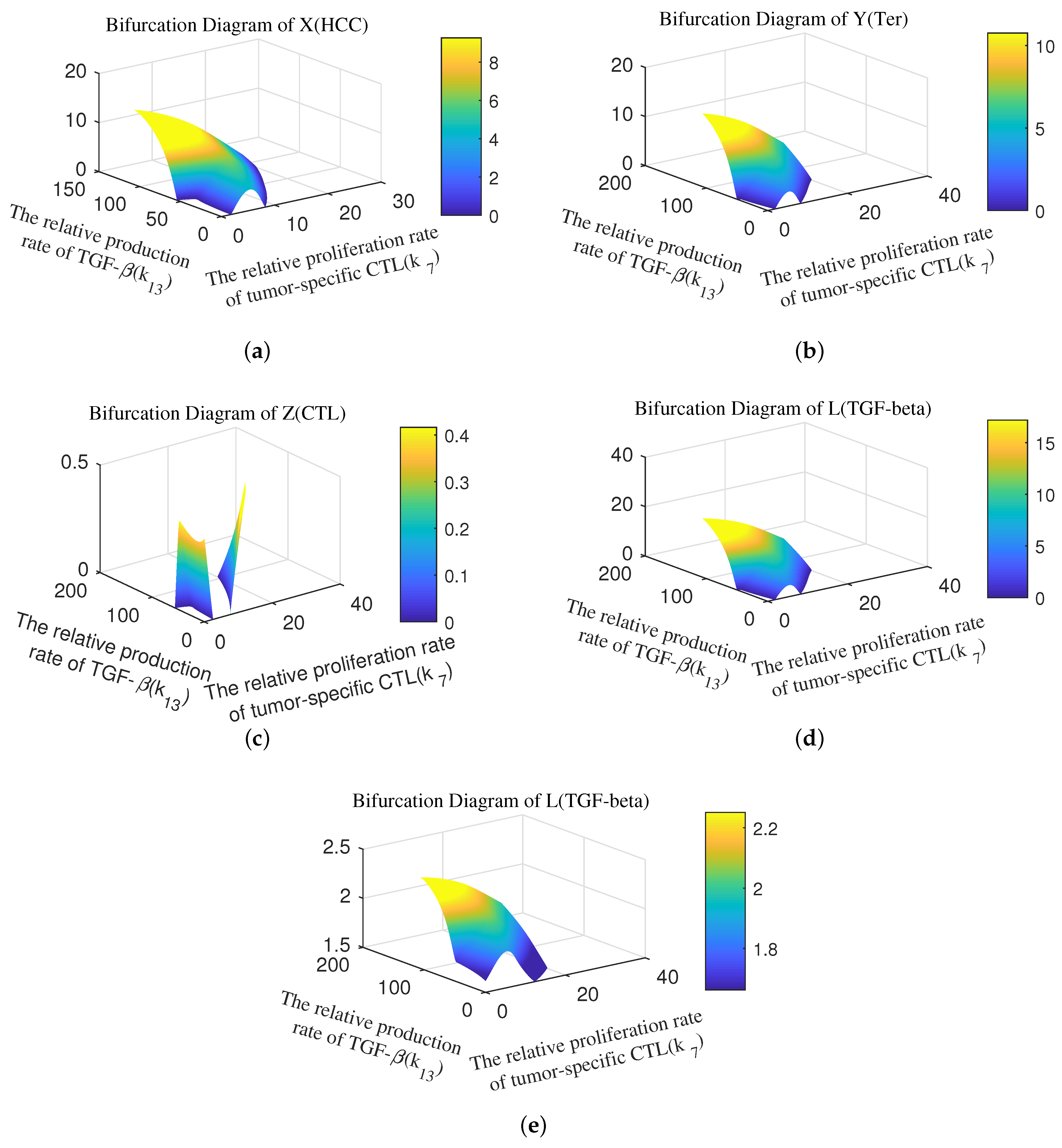
4.3. One-Parameter Bifurcation Analysis Reveals the Significant Effect of Immunity Activation

We performed a one-parameter study with a focus on $k_7$, which indicates the ratio of CTL proliferation rate to CTL killing rate, in order to further examine the impact of CTL activation on the growth of HCC. Figure 5a,b show how the ODE model (Equation (2)) behaves when it bifurcates with regard to $k_7$. The model contains one stable equilibrium point, $E_1$, when $k_7<7.95$. The system experiences bifurcation when $k_7$ steadily rises, producing two stable equilibrium points and one unstable equilibrium point. With greater values of $k_7$, the bigger stable equilibrium point grows while the smaller one stays constant. A limit point and a branch point are found at $k_7$ = 7.95 and 9.27, respectively. The bigger stable equilibrium point increases as $k_7$ is raised, whereas the smaller stable equilibrium point decreases. Similar bifurcation trend with regard to $k_9$ (the relative TGF-$\beta$-induced differentiation of CTL) is shown in Figure 5c,d. The system has one stable equilibrium point, $E_1$, when $k_9>41.46$. Bifurcation, which creates one unstable equilibrium point and two stable equilibrium points, happens when $k_9$ drops. Lower values of $k_9$ result in a smaller stable equilibrium point while the bigger one diminishes. A limit point and a branch point are found at $k_9$ = 41.46 and 38.2, respectively. The bigger stable equilibrium point rises when $k_9$ is further reduced, whereas the smaller stable equilibrium point falls. For the remaining 14 parameters, we also conducted bifurcation analysis, but no appreciable bifurcation occurrences were observed.

For various choices of $k_7$, numerical simulations show how X (HCC) changes from a highly stable equilibrium state to an unstable state and then goes to a low equilibrium state. We link these several states, defined by varying levels of X (HCC), with the “escape”, “equilibrium”, and “elimination” stages of the immunoediting concept. This shows that HCC elimination depends on CTL activation or cellular immunity as indicated by CTL accumulation. However, for $k_9$, one can come to the opposite conclusion. To manage cancer, we can change $k_7$ within the low steady-state interval $[-\infty ,38.2]$ or $k_9$ throughout the low steady-state period $[9.27,+\infty ]$.

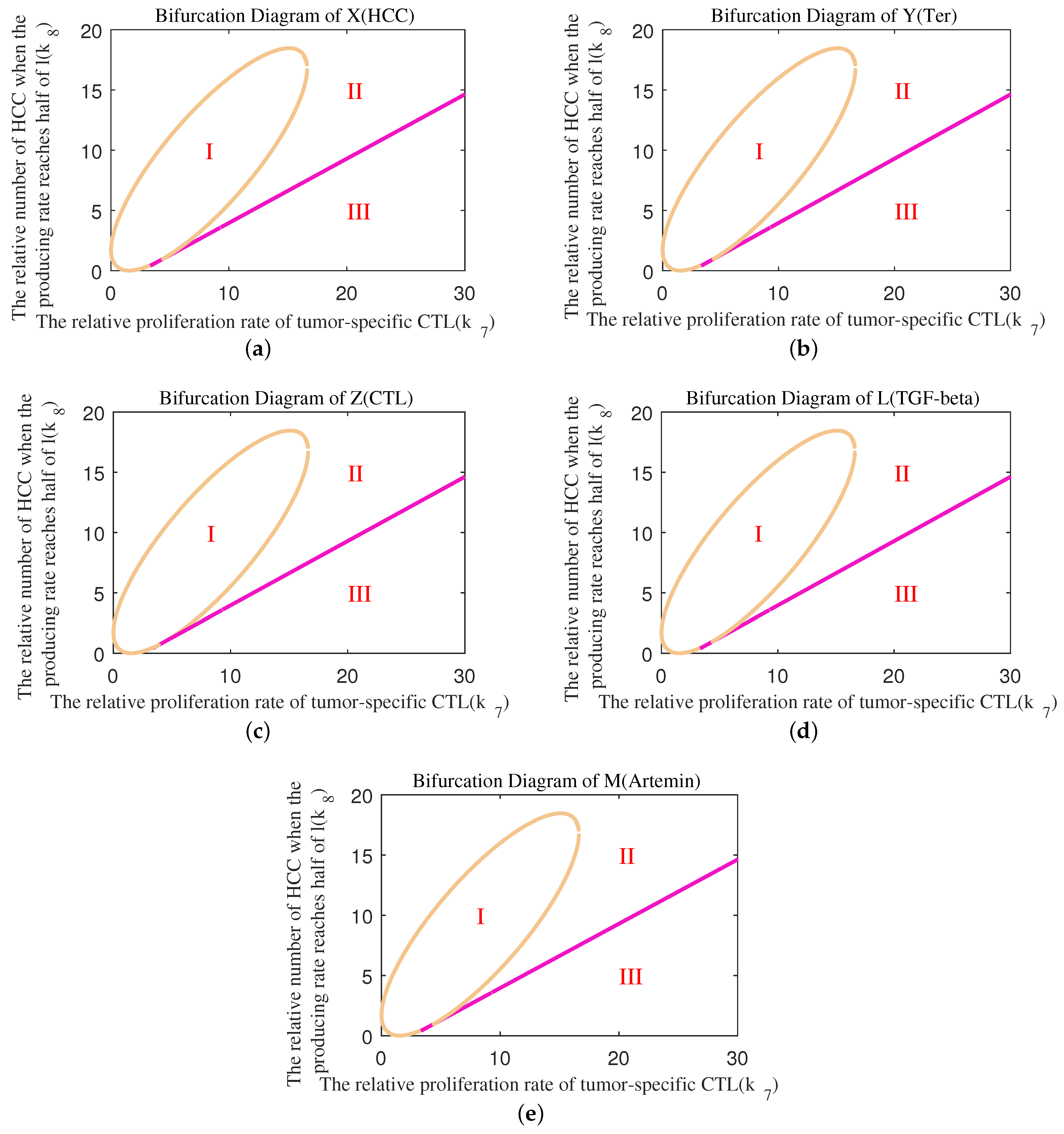
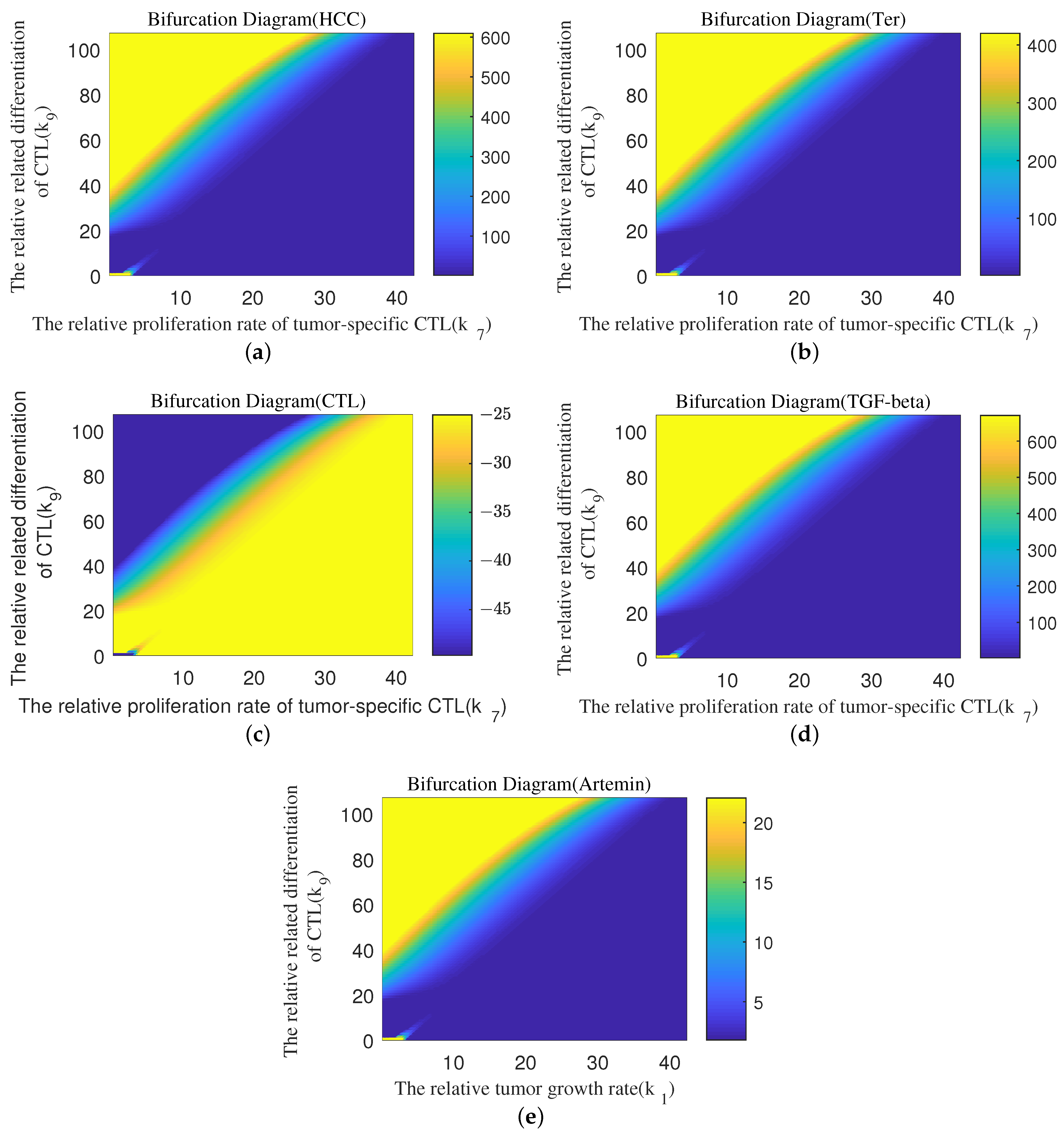
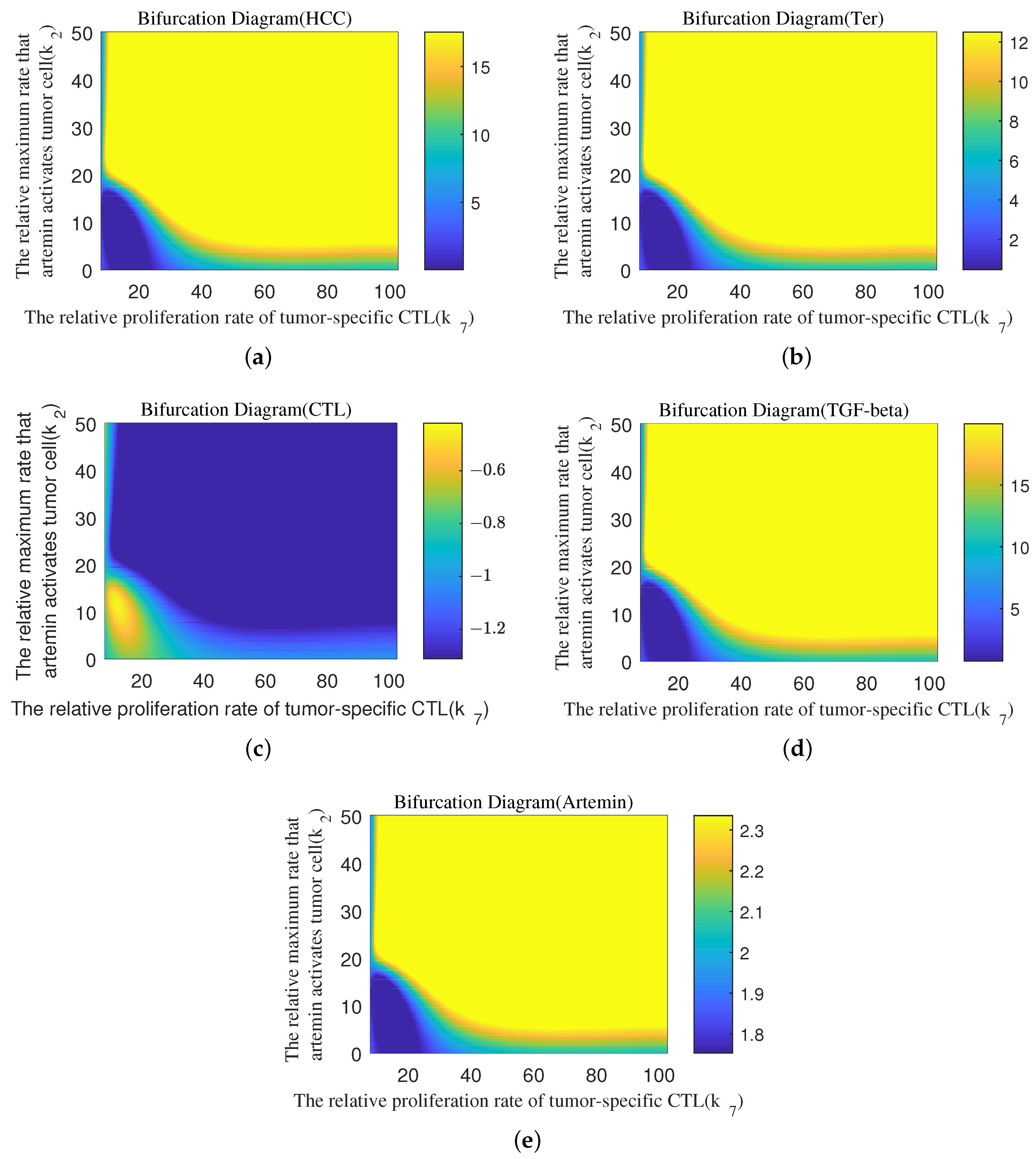
4.4. Quantitative Analysis of Parameter Interactions

We are interested in learning how various biological processes impact HCC development while the immune response is keeping an eye on the system (2). Figure 6a,b show that X (HCC) maintains a high steady state when $k_7$ is within the range [0, 7.95] and $k_9$ is less than 1. X (HCC) remains in a low steady state when $k_9$ varies in the range [1, 38.2], regardless of how $k_7$ varies. However, as $k_7$ rises, the system shifts from a high to a low steady state when $k_9$ is in the range $[38.2,+\infty ]$. In Figure 7a, the system displays a low level of X (HCC) when $k_7$ is below the 12 threshold regardless of how $k_1$ varies. In contrast, a high amount of X is kept when $k_7$ is greater than 13. This shows that, in comparison to CTL activation, the growth rate of HCC does not affect on HCC progression. On the other hand, if $k_9$ is below 10, the carcinoma level is persistently high regardless of changes in $k_1$, and if $k_9$ is above 25, HCC remains at a low steady-state regardless of changes in $k_1$ (Figure 7c). In Figure 7b, a low steady state is maintained when $k_6$ surpasses 1, independent of changes in $k_7$, but a high steady state is produced when $k_6$ remains below 0.5. When $k_7$ is smaller than 9.27, Figure 7d shows a different pattern in which the system changes from a low to a high steady state as $k_{15}$ rises. However, the system remains in a low steady-state regardless of changes in $k_{15}$ when $k_7$ is greater than 9.27.

The impact of $k_2$ and $k_7$ on the five variables is depicted in Figure 8. It follows the same pattern for X, Y, L, and M. Regardless of changes in $k_2$, the system maintains a low steady state when $k_7$ is within the range [0, 9.72]. But when $k_2$ is between [0, 20] and $k_7$ is greater than 9.72, HCC progressively moves from a low to a high steady state as $k_7$ rises. The system continues in a high steady state when $k_2$ is higher than 20 and $k_7$ is higher than 9.72. Notably, given the shift in Z, the other variables remain in low steady-state regions when $k_2$ and $k_7$ fall within the circular high steady-state area $[0,20]\times [0,20]$.

In Figure 9a,b, we suggest that $k_7$ within the range [0, 9.72] and $k_{13}$ within the range [0, 80] can be controlled to successfully control HCC. The two-dimensional region is additionally divided into three parts by $k_7$ and $k_8$, one of which forms a unique circular area. X (HCC) must be smaller than 1 in accordance with nondimensionalized parameters and fundamental biological concepts. We can see an unstable equilibrium point ($E_0$) in the region I and both stable and unstable equilibrium points ($E_0$) in the region II in Figure 9c,d. This finding also applies to area III. We can successfully treat cancer and reach a low stable state by modulating $k_7$ and $k_8$ in regions II and III.

Our model reveals that immune-suppressive mechanisms regulated by the tumor itself, such as TGF-$\beta$ secretion that converts CTLs into regulatory T-cells, resulting in the challenge of higher CTL activation thresholds. This explains why the number of T regulatory cells (Tregs) increases in both peripheral blood and tumors, often associated with poor prognosis [35,36].

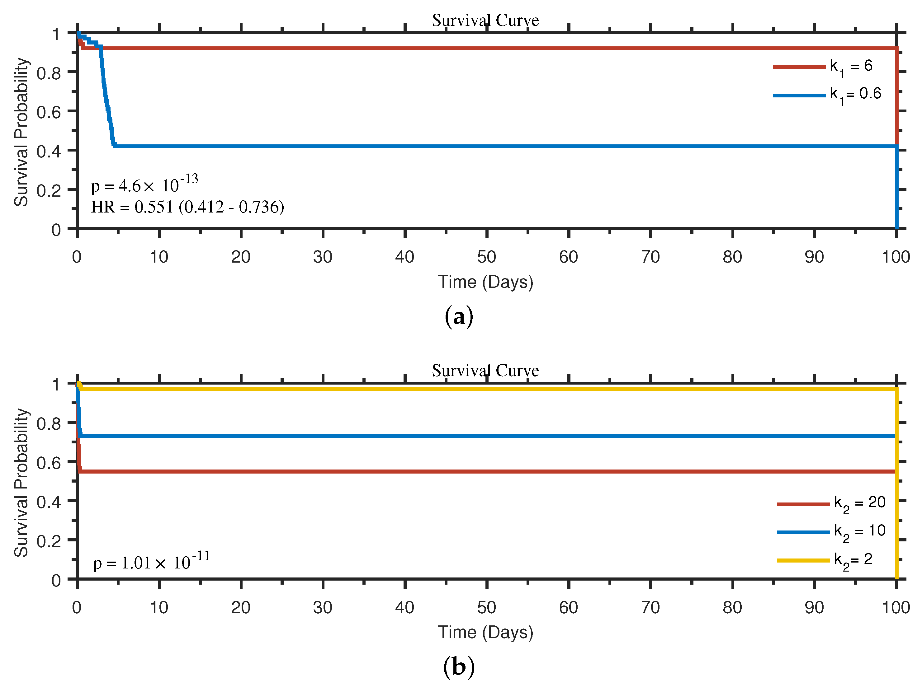
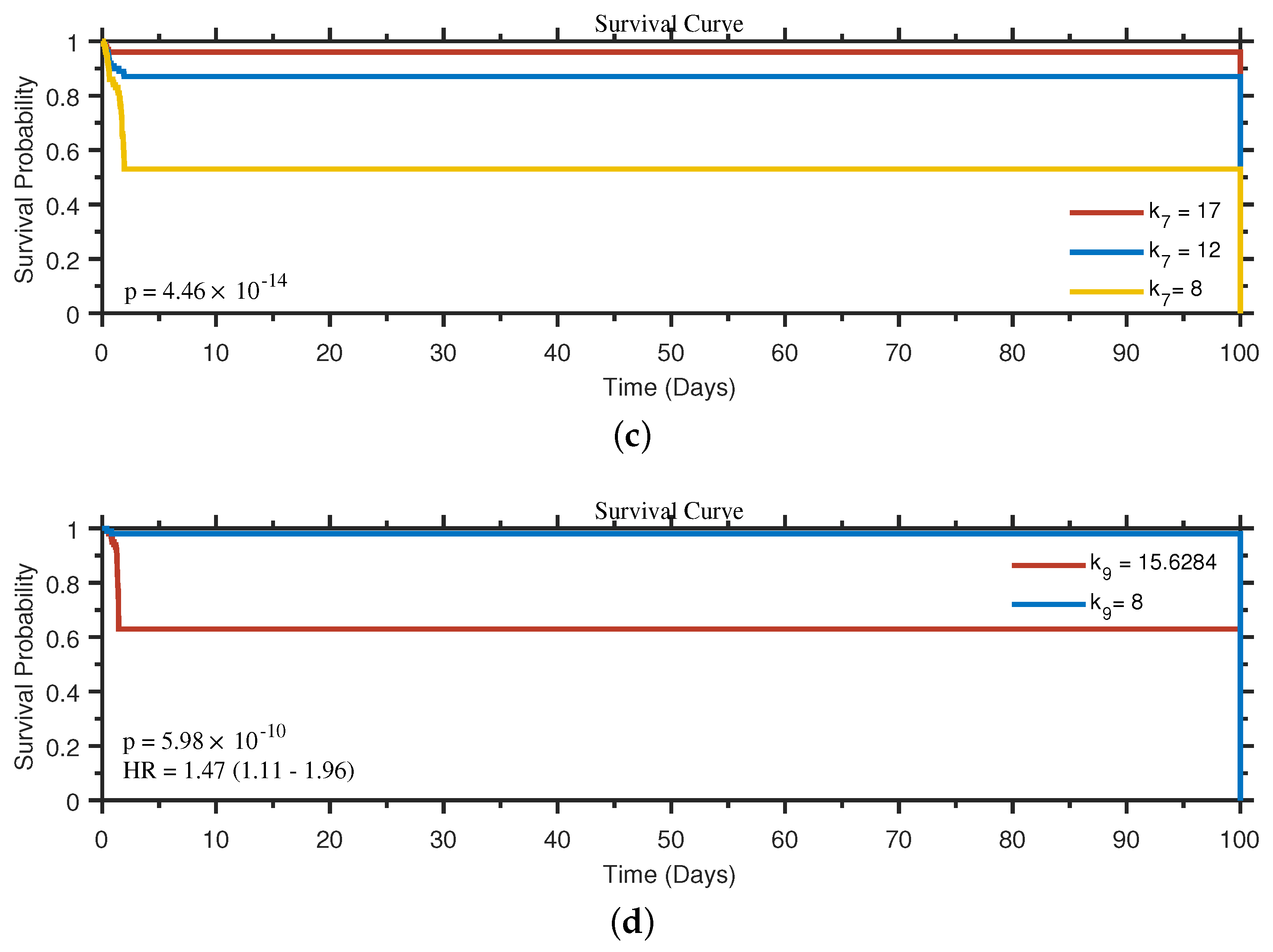
4.5. Survival Analysis Based on the Influence of Biological Processes

Although the system does not change from having a high level of X (HCC) to having a low level of relative HCC cell counts as a result of the increase in $k_4$ (relative death rate of HCC) (Figure 4d,e), this does not mean that treatments that aim to destroy HCC, such as radiotherapy, is worthless for patients. With varied $k_4$ and $k_7$ values, we ran simulations of the system dynamics and noted the moment at which the relative HCC cell counts first hit one, which we took to be the death threshold of X. An individual’s survival time is represented by the period that has been documented.

Figure 10 shows that when $k_7$ surpasses 20 (equivalent to the cutoff in Figure 5b), an individual will die from HCC. On the other hand, if $k_7$ is lower than 9.72, the person will pass away from cancer. It’s interesting to note that raising $k_4$ can prolong the interval of X (HCC) in the low steady state, prolonging individual survival time. This result defies the common sense that suggests a larger relative HCC death rate is preferable when trying to slow tumor growth. It highlights the fact that cancer, like HCC, is a systemic disease that requires dynamic analysis techniques. Overall, a decline in $k_7$ increases survival time.

We created 100 individuals with distributed initial values and recorded their survival times under various settings to obtain the survival time of individuals through numerical simulations. When comparing the relative HCC proliferation rates ($k_1$) of these people across time, we discovered that a lower $k_1$ correlates with a lower survival rate. According to our hypothesis, rapid HCC proliferation causes CTL to become activated and accumulate, which in turn speeds up the removal of HCC (Figure 4a and Figure 11a). The long-term survival rate is not encouraging (relative time 100), notwithstanding the possibility that varying relative HCC proliferation rates could affect short-term survival rates. In line with the finding that serum artemin encourages HCC progression [24], we also noticed that relative artemin-induced HCC proliferation lowers the survival rate (Figure 11b). We conclude that the proliferation rate of CTL has a considerable effect on population survival rates in light of the large influence of $k_7$ on survival time (Figure 5a). Figure 11c shows that increased CTL proliferation rates are associated with observable increases in long-term survival rates. Additionally, we found that the TGF-$\beta$-induced CTL differentiation rate has a significant impact on survival rates (Figure 11d). Figure 12 shows the survival curves of Ter cells, CTLs, serum artemin, and serum TGF-$\beta$ under various starting circumstances. For all variables of the double parameter you can refer to Figure A1, Figure A2, Figure A3, Figure A4, Figure A5, Figure A6, Figure A7 and Figure A8 in the Appendix B.

5. Conclusions & Discussion

In this study, we developed a mathematical ODE model based on the core cancer-immune interaction network, which includes HCC, Ter cells, CTL, serum TGF-$\beta$, and serum artemin. Through simulations, we validated the accuracy of the model and the constructed network.

Our research showed that altering the final stage of HCC development would not be possible by reducing HCC proliferation or raising HCC mortality rates (Figure 4a,f). In order to properly treat HCC, standard therapies such as medication therapy, chemotherapy, and surgical resection have inherent limitations. Our findings highlight the crucial role of cellular immunity in the therapy of HCC and show that activating CTL is the most effective strategy to eradicate HCC (Figure 5). Apart from $k_7$ (the ratio of CTL proliferation rate to death rate) and $k_9$ (related to TGF-$\beta$-mediated CTL differentiation), changes in the other 14 parameters did not result in transitions from an equilibrium state with high HCC cell counts to an equilibrium state with low relative HCC cell counts, according to the bifurcation analysis of the 16 parameters. It’s interesting to note that HCC was shown to be in an intermediate unstable condition, which matches the idea of an “equilibrium state” in the cancer immunoediting theory. Inhibiting HCC growth and raising the mortality rate of HCC had limitations in identifying the long-term steady state of HCC cell counts, but they had a considerable impact on short-term individual survival, according to a survival rate analysis of simulation data from the model (Figure 11a,b). Additionally, survival curves under various beginning circumstances confirmed the common sense observation that people with more HCC cells and fewer CTLs typically live shorter lifetimes (Figure 12). We deduced from Figure 11c that the activation of cellular immunity, or a faster creation and accumulation of CTLs (higher proliferation constant l), would inhibit and suppress the growth of HCC. Additionally, only when CTL proliferation was sufficiently triggered did the presence of serum TGF-$\beta$, a protein associated with hepatocellular cancer, affect survival time. Through a linear function, CTL activation and differentiation together impacted the development of HCC (Figure A8b,c).

Although substantial progress has been achieved by clinical and theoretical studies, the molecular, cellular, and environmental factors influencing HCC pathogenesis are still poorly understood. In addition, current therapeutic options such as surgical resection, liver transplantation, and ablative therapies, only partially improve certain clinical outcomes [37,38]. This research offers fresh perspectives and approaches to improve our comprehension of the driving forces behind the development of HCC. To analyze systemic disorders like HCC, mathematical modeling is a useful technique in our opinion.

The synergy between mathematics and biology is particularly evident in the development of computational models. These models act as virtual laboratories, enabling researchers to simulate complex biological processes, understand underlying mechanisms, and predict outcomes under various conditions. In this article, we highlight key areas where mathematical modeling can enhance our approach to cancer treatment and prediction.

The approach in this paper primarily relies on mathematical modeling which is mainly from a dynamical perspective, and we can consider high throughput based data in the future. This integrated approach combines data, such as cancer volume, high-throughput screening data, single-cell data, microarray datasets, and RNA seq data, with mathematical models to predict future cancer developments and devise effective treatment plans [26,39]. The symbiosis between mathematical modeling and data analysis, encompassing techniques from sequencing data analysis to cancer volume measurements, can provide robust evidence for cancer diagnosis and screening strategies in the realm of medical research. However, it is important to note that integrating diverse data sources poses several challenges, including the need to harmonize disparate data types and select appropriate modeling techniques. Moreover, we anticipate the incorporation of targeted therapies, such as CAR-T cells and CAR-NK cells, which are promising cellular immunotherapy approaches that identify specific tumor antigens. By combining these targeted therapies with other treatment modalities, including CTL, drug therapy, and non-systemic chemotherapy, and incorporating various data types into our modeling, we can pave the way for interdisciplinary research. Recent advances in understanding molecular and cellular mechanisms, including immune escape, tumorigenesis, drug resistance, and cancer metastasis, further underscore the importance of this interdisciplinary approach. Ultimately, combination therapy offers distinct advantages over single treatment strategies and holds promise for improving cancer treatment outcomes.

In many biological models, time delays are a common phenomenon that can significantly impact the stability of systems over time [40,41,42]. It is essential to analyze the existence of bounded invariant sets, which represent sets of values that remain within certain bounds over time, and nonnegative system solutions, which are solutions that remain nonnegative for all time. This analysis helps in assessing local and global stability in biological systems. When dealing with a system exhibiting the same time delay, one may refer to the proof procedure outlined in Reference [43]. Conversely, for systems with different time delays, the findings and proof methods presented in References [44,45] can be applied. Additionally, by introducing periodic dynamics [46,47] through the incorporation of periodic components into the model, researchers can calculate important parameters such as the basic regeneration number and determine the possibilities of extinction and persistence of equilibrium solutions.

Numerous functions may be used to describe biological relationships, and even the same function can be expressed in several ways. Fractional order differential operators, known for their ability to succinctly describe complex mechanical and physical processes, have become essential tools in mathematical modeling. They offer accurate descriptions of processes with historical memory and spatial global correlation. Further research into the bifurcation problem of fractional order models, including their application to model (1), represents a promising future direction [48,49,50]. Additionally, exploring the theoretical aspects of fractional order models warrants consideration.

References

1. Llovet, J.M.; Kelley, R.K.; Villanueva, A.; Singal, A.G.; Pikarsky, E.; Roayaie, S.; Lencioni, R.; Koike, K.; Zucman-Rossi, J.; Finn, R.S. Hepatocellular carcinoma. Nat. Rev. Dis. Prim. 2021, 7, 6. [Google Scholar] [CrossRef]
2. Vogel, A.; Meyer, T.; Sapisochin, G.; Salem, R.; Saborowski, A. Hepatocellular carcinoma. Lancet 2022, 400, 1345–1362. [Google Scholar] [CrossRef] [PubMed]
3. Gingold, J.A.; Zhu, D.; Lee, D.F.; Kaseb, A.; Chen, J. Genomic Profiling and Metabolic Homeostasis in Primary Liver Cancers. Trends Mol. Med. 2018, 24, 395–411. [Google Scholar] [CrossRef]
4. The Cancer Genome Atlas Research Network. Comprehensive and integrative genomic characterization of hepatocellular carcinoma. Cell 2017, 176, 1327–1341.e23. [Google Scholar] [CrossRef]
5. Lin, H.; Xie, Y.; Kong, Y.; Yang, L.; Li, M. Identification of molecular subtypes and prognostic signature for hepatocellular carcinoma based on genes associated with homologous recombination deficiency. Sci. Rep. 2021, 11, 24022. [Google Scholar] [CrossRef] [PubMed]
6. Hajibabaie, F.; Abedpoor, N.; Haghjooy Javanmard, S.; Hasan, A.; Sharifi, M.; Rahimmanesh, I.; Shariati, L.; Makvandi, P. The molecular perspective on the melanoma and genome engineering of T-cells in targeting therapy. Environ. Res. 2023, 237, 116980. [Google Scholar] [CrossRef] [PubMed]
7. O’Donnell, J.S.; Teng, M.W.; Smyth, M.J. Cancer immunoediting and resistance to T cell-based immunotherapy. Nat. Rev. Clin. Oncol. 2019, 16, 151–167. [Google Scholar] [CrossRef]
8. Łuksza, M.; Sethna, Z.M.; Rojas, L.A.; Lihm, J.; Bravi, B.; Elhanati, Y.; Soares, K.; Amisaki, M.; Dobrin, A.; Hoyos, D.; et al. Neoantigen quality predicts immunoediting in survivors of pancreatic cancer. Nature 2022, 606, 389–395. [Google Scholar] [CrossRef]
9. Gubin, M.M.; Vesely, M.D. Cancer Immunoediting in the Era of Immuno-oncology. Clin. Cancer Res. 2022, 28, 3917–3928. [Google Scholar] [CrossRef]
10. Sangro, B.; Sarobe, P.; Hervás-Stubbs, S.; Melero, I. Advances in immunotherapy for hepatocellular carcinoma. Nat. Rev. Gastroenterol. Hepatol. 2021, 18, 525–543. [Google Scholar] [CrossRef] [PubMed]
11. Pinato, D.J.; Guerra, N.; Fessas, P.; Murphy, R.; Mineo, T.; Mauri, F.A.; Mukherjee, S.K.; Thursz, M.; Wong, C.N.; Sharma, R.; et al. Immune-based therapies for hepatocellular carcinoma. Oncogene 2020, 39, 3620–3637. [Google Scholar] [CrossRef]
12. Ruf, B.; Heinrich, B.; Greten, T.F. Immunobiology and immunotherapy of HCC: Spotlight on innate and innate-like immune cells. Cell. Mol. Immunol. 2021, 18, 112–127. [Google Scholar] [CrossRef]
13. Tsuchiya, N.; Sawada, Y.; Endo, I.; Uemura, Y.; Nakatsura, T. Potentiality of immunotherapy against hepatocellular carcinoma. World J. Gastroenterol. 2015, 21, 10314–10326. [Google Scholar] [CrossRef] [PubMed]
14. Hepatobiliary malignancies have distinct peripheral myeloid-derived suppressor cell signatures and tumor myeloid cell profiles. Sci. Rep. 2020, 10, 18848. [CrossRef] [PubMed]
15. Mantovani, S.; Oliviero, B.; Varchetta, S.; Mele, D.; Mondelli, M.U. Natural Killer Cell Responses in Hepatocellular Carcinoma: Implications for Novel Immunotherapeutic Approaches. Cancers 2020, 12, 926. [Google Scholar] [CrossRef]
16. Kalathil, S.G.; Thanavala, Y. Natural Killer Cells and T Cells in Hepatocellular Carcinoma and Viral Hepatitis: Current Status and Perspectives for Future Immunotherapeutic Approaches. Cells 2021, 10, 1332. [Google Scholar] [CrossRef] [PubMed]
17. Langhans, B.; Nischalke, H.D.; Krämer, B.; Dold, L.; Lutz, P.; Mohr, R.; Vogt, A.; Toma, M.; Eis-Hübinger, A.M.; Nattermann, J.; et al. Role of regulatory T cells and checkpoint inhibition in hepatocellular carcinoma. Cancer Immunol. Immunother. 2019, 68, 2055–2066. [Google Scholar] [CrossRef] [PubMed]
18. Yu, S.; Wang, Y.; Hou, J.; Li, W.; Wang, X.; Xiang, L.; Tan, D.; Wang, W.; Jiang, L.; Claret, F.X.; et al. Tumor-infiltrating immune cells in hepatocellular carcinoma: Tregs is correlated with poor overall survival. PLoS ONE 2020, 15, e0231003. [Google Scholar] [CrossRef] [PubMed]
19. Cheng, A.L.; Hsu, C.; Chan, S.L.; Choo, S.P.; Kudo, M. Challenges of combination therapy with immune checkpoint inhibitors for hepatocellular carcinoma. J. Hepatol. 2020, 72, 307–319. [Google Scholar] [CrossRef]
20. Wu, T.C.; Shen, Y.C.; Cheng, A.L. Evolution of systemic treatment for advanced hepatocellular carcinoma. Kaohsiung J. Med. Sci. 2021, 37, 643–653. [Google Scholar] [CrossRef] [PubMed]
21. Finn, R.S.; Zhu, A.X. Evolution of Systemic Therapy for Hepatocellular Carcinoma. Hepatology 2021, 73, 150–157. [Google Scholar] [CrossRef] [PubMed]
22. Llovet, J.M.; Pinyol, R.; Kelley, R.K.; El-Khoueiry, A.; Reeves, H.L.; Wang, X.W.; Gores, G.J.; Villanueva, A. Molecular pathogenesis and systemic therapies for hepatocellular carcinoma. Nat. Cancer 2022, 3, 386–401. [Google Scholar] [CrossRef] [PubMed]
23. Llovet, J.M.; Castet, F.; Heikenwalder, M.; Maini, M.K.; Mazzaferro, V.; Pinato, D.J.; Pikarsky, E.; Zhu, A.X.; Finn, R.S. Immunotherapies for hepatocellular carcinoma. Nat. Rev. Clin. Oncol. 2022, 19, 151–172. [Google Scholar] [CrossRef]
24. Han, Y.; Liu, Q.; Hou, J.; Gu, Y.; Zhang, Y.; Chen, Z.; Fan, J.; Zhou, W.; Qiu, S.; Zhang, Y.; et al. Tumor-Induced Generation of Splenic Erythroblast-like Ter-Cells Promotes Tumor Progression. Cell 2018, 173, 634–648. [Google Scholar] [CrossRef]
25. Shen, J.; Yao, Z.; Tan, X.; Zou, X. Mathematical Modeling and Dynamical Analysis for Tumor Cells and Tumor Propagating Cells Controlled by G9a Inhibitors. Int. J. Bifurc. Chaos 2023, 33, 2350006. [Google Scholar] [CrossRef]
26. Tu, X.; Zhang, Q.; Zhang, W.; Zou, X. Single-cell data-driven mathematical model reveals possible molecular mechanisms of embryonic stem-cell differentiation. Math. Biosci. Eng. 2019, 16, 5877–5896. [Google Scholar] [CrossRef]
27. Ait-Oudhia, S.; Mager, D.E.; Pokuri, V.; Tomaszewski, G.; Groman, A.; Zagst, P.; Fetterly, G.; Iyer, R. Bridging sunitinib exposure to time-to-tumor progression in hepatocellular carcinoma patients with mathematical modeling of an angiogenic biomarker. CPT Pharmacometrics Syst. Pharmacol. 2016, 5, 297–304. [Google Scholar] [CrossRef]
28. Saidak, Z.; Giacobbi, A.S.; Louandre, C.; Sauzay, C.; Mammeri, Y.; Galmiche, A. Mathematical modelling unveils the essential role of cellular phosphatases in the inhibition of RAF-MEK-ERK signalling by sorafenib in hepatocellular carcinoma cells. Cancer Lett. 2017, 392, 1–8. [Google Scholar] [CrossRef] [PubMed]
29. Sung, W.; Grassberger, C.; McNamara, A.L.; Basler, L.; Ehrbar, S.; Tanadini-Lang, S.; Hong, T.S.; Paganetti, H. A tumor-immune interaction model for hepatocellular carcinoma based on measured lymphocyte counts in patients undergoing radiotherapy. Radiother. Oncol. 2020, 151, 73–81. [Google Scholar] [CrossRef]
30. Sung, W.; Hong, T.S.; Poznansky, M.C.; Paganetti, H.; Grassberger, C. Mathematical Modeling to Simulate the Effect of Adding Radiation Therapy to Immunotherapy and Application to Hepatocellular Carcinoma. Int. J. Radiat. Oncol. Biol. Phys. 2022, 112, 1055–1062. [Google Scholar] [CrossRef]
31. Unni, P.; Seshaiyer, P. Mathematical Modeling, Analysis, and Simulation of Tumor Dynamics with Drug Interventions. Comput. Math. Methods Med. 2019, 2019, 4079298. [Google Scholar] [CrossRef] [PubMed]
32. Wilson, S.; Levy, D. A Mathematical Model of the Enhancement of Tumor Vaccine Efficacy by Immunotherapy. Bull. Math. Biol. 2012, 74, 1485–1500. [Google Scholar] [CrossRef]
33. Xue, V.W.; Chung, J.Y.F.; Córdoba, C.A.G.; Cheung, A.H.K.; Kang, W.; Lam, E.W.F.; Leung, K.T.; To, K.F.; Lan, H.Y.; Tang, P.M.K. Transforming Growth Factor-β: A Multifunctional Regulator of Cancer Immunity. Cancers 2020, 12, 3099. [Google Scholar] [CrossRef] [PubMed]
34. Marino, S.; Hogue, I.B.; Ray, C.J.; Kirschner, D.E. A methodology for performing global uncertainty and sensitivity analysis in systems biology. J. Theor. Biol. 2008, 254, 178–196. [Google Scholar] [CrossRef] [PubMed]
35. Teng, C.F.; Li, T.C.; Wang, T.; Liao, D.C.; Wen, Y.H.; Wu, T.H.; Wang, J.; Wu, H.C.; Shyu, W.C.; Su, I.J.; et al. Increased infiltration of regulatory T cells in hepatocellular carcinoma of patients with hepatitis B virus pre-S2 mutant. Sci. Rep. 2021, 11, 1136. [Google Scholar] [CrossRef] [PubMed]
36. Sachdeva, M.; Arora, S. Prognostic role of immune cells in hepatocellular carcinoma. EXCLI J. 2020, 19, 718–733. [Google Scholar] [CrossRef] [PubMed]
37. Cucarull, B.; Tutusaus, A.; Rider, P.; Hernáez-Alsina, T.; Cuño, C.; García de Frutos, P.; Colell, A.; Marí, M.; Morales, A. Hepatocellular Carcinoma: Molecular Pathogenesis and Therapeutic Advances. Cancers 2022, 14, 621. [Google Scholar] [CrossRef] [PubMed]
38. Da, B.L.; Suchman, K.I.; Lau, L.; Rabiee, A.; He, A.R.; Shetty, K.; Yu, H.; Wong, L.L.; Amdur, R.L.; Crawford, J.M.; et al. Pathogenesis to management of hepatocellular carcinoma. Genes Cancer 2022, 13, 72–87. [Google Scholar] [CrossRef]
39. Qiu, X.; Zhang, Y.; Martin-Rufino, J.D.; Weng, C.; Hosseinzadeh, S.; Yang, D.; Pogson, A.N.; Hein, M.Y.; Hoi (Joseph) Min, K.; Wang, L.; et al. Mapping transcriptomic vector fields of single cells. Cell 2022, 185, 690–711.e45. [Google Scholar] [CrossRef]
40. Khajanchi, S.; Nieto, J.J. Mathematical modeling of tumor-immune competitive system, considering the role of time delay. Appl. Math. Comput. 2019, 340, 180–205. [Google Scholar] [CrossRef]
41. Nouni, A.; Hattaf, K.; Yousfi, N. Dynamics of a mathematical model for cancer therapy with oncolytic viruses. Commun. Math. Biol. Neurosci. 2019, 237. [Google Scholar] [CrossRef]
42. Nouni, A.; Hattaf, K.; Yousfi, N. Dynamics of a Virological Model for Cancer Therapy with Innate Immune Response. Complexity 2020, 2020, 8694821. [Google Scholar] [CrossRef]
43. Liu, Z.; Li, W.; Xu, C.; Liu, C.; Mu, D.; Xu, M.; Ou, W.; Cui, Q. Bifurcation mechanism and hybrid control strategy of a finance model with delays. Bound. Value Probl. 2023, 2023, 82. [Google Scholar] [CrossRef]
44. Li, P.; Gao, R.; Xu, C.; Shen, J.; Ahmad, S.; Li, Y. Exploring the Impact of Delay on Hopf Bifurcation of a Type of BAM Neural Network Models Concerning Three Nonidentical Delays. Neural Process. Lett. 2023. [Google Scholar] [CrossRef]
45. Ou, W.; Xu, C.; Cui, Q.; Liu, Z.; Pang, Y.; Farman, M.; Ahmad, S.; Zeb, A. Mathematical study on bifurcation dynamics and control mechanism of tri-neuron bidirectional associative memory neural networks including delay. Math. Methods Appl. Sci. 2023, 1–25. [Google Scholar] [CrossRef]
46. Huang, M.; Wu, S.L.; Zhao, X.Q. Propagation Dynamics for Time–Space Periodic and Partially Degenerate Reaction–Diffusion Systems with Time Delay. J. Dyn. Differ. Equat. 2023. [Google Scholar] [CrossRef]
47. Malinzi, J.; Soltani, M. Mathematical Analysis of a Mathematical Model of Chemovirotherapy: Effect of Drug Infusion Method. Comput. Math. Methods Med. 2019, 2019, 15–20. [Google Scholar] [CrossRef]
48. Li, P.; Peng, X.; Xu, C.; Han, L.; Shi, S. Novel extended mixed controller design for bifurcation control of fractional-order Myc/E2F/miR-17-92 network model concerning delay. Math. Methods Appl. Sci. 2023, 1–21. [Google Scholar] [CrossRef]
49. Xu, C.; Liu, Z.; Li, P.; Yan, J.; Yao, L. Bifurcation Mechanism for Fractional-Order Three-Triangle Multi-delayed Neural Networks. Neural Process. Lett. 2022, 55, 6125–6151. [Google Scholar] [CrossRef]
50. Li, P.; Lu, Y.; Xu, C.; Ren, J. Insight into Hopf Bifurcation and Control Methods in Fractional Order BAM Neural Networks Incorporating Symmetric Structure and Delay. Cogn. Comput. 2023, 1–43. [Google Scholar] [CrossRef]
Figure 1. Illustration of Ter-cells-HCC-CTLs-TGF- β -Artemin system. The core regulatory networks we have constructed. The arrows indicate promotion, while the blunt edges indicate inhibition.
Mathematics 11 04261 g001
Figure 2. The sensitivity analysis to the perturbation of parameters in the model. (a) The sensitivity of X (HCC) to every single parameter. (b) The Y (Ter) sensitivity to all parameters. (c) The Z (CTL) sensitivity to all factors. (d) The L (TGF- β ) sensitivity with respect to all parameters. (e) The M (Artemin) sensitivity with regard to all parameters. The sensitivity of the variable at relative times 100, 200, 500 is depicted by each of the three colors.
Mathematics 11 04261 g002
Figure 3. The curves in different color with different initial points finally approach the same equilibrium point E 1 ( 0.43 , 0.73 , 0.08 ) in the three-dimensional space formed by variables X, Y and Z.
Mathematics 11 04261 g003
Figure 4. Effects of Therapies on Relative HCC Cell Counts. (a) Simulation of X (HCC) with varying relative proliferation rates. (b) and (c) Changing the relative proliferation rate of HCC at relative times 4.887 and 9.774 to simulate the effect of anti-proliferation drugs on tumors, respectively. (d) Simulation of X (HCC) with different relative killing rates. (e) Effect of HCC resection at relative time 4.887 of HCC development. (f) Changing the relative killing rate of HCC at relative times 3 and 8 to simulate the effect of chemotherapy on tumors. (g) and (h) Simulating the effect of immune system activation on X (HCC) at relative times 0 and 4.887, respectively.
Mathematics 11 04261 g004aMathematics 11 04261 g004b
Figure 5. (a) Bifurcation diagram with respect to k 7 . (b) Dynamics of HCC with increasing k 7 (represented in different colors). (c) Bifurcation diagram with respect to k 9 . (d) Dynamics of HCC with different k 9 (represented in different colors). LP denotes a limit point, and BR denotes a branch point.
Mathematics 11 04261 g005aMathematics 11 04261 g005b
Figure 6. The steady level of X (HCC) and Z (CTL) of the model with different values k 7 and k 9 . (a) The steady level of X (HCC) of the model with different values k 7 and k 9 . (b) The steady level of Z (CTL) of the model with different values k 7 and k 9 . The blue region indicates a low level of X (or Z) and the yellow region indicates a high level of X (or Z).
Mathematics 11 04261 g006
Figure 7. (a) The steady level of X (HCC) of the model with different values k 7 and k 1 . (b) The steady level of X (HCC) of the model with different values k 7 and k 6 . (c) The steady level of X (HCC) of the model with different values k 9 and k 1 . (d) The steady level of X (HCC) of the model with different values k 7 and k 15 . The blue region indicates a low level of X and the yellow region indicates a high level of X.
Mathematics 11 04261 g007
Figure 8. Bifurcation diagram of k 7 and k 2 . (a) The steady level of X (HCC) of the model with different values k 7 and k 2 . (b) The steady level of Y (Ter) of the model with different values k 7 and k 2 . (c) The steady level of Z (CTL) of the model with different values k 7 and k 2 . (d) The steady level of L (TGF- β ) of the model with different values k 7 and k 2 . (e) The steady level of M (Artemin) of the model with different values k 7 and k 2 .
Mathematics 11 04261 g008
Figure 9. Bifurcation diagram of two parameters. (a) The steady level of X (HCC) of the model with different values k 7 and k 13 . (b) The steady level of Z (CTL) of the model with different values k 7 and k 13 . (c) The steady level of X (HCC) of the model with different values k 7 and k 8 . (d) The steady level of Z (CTL) of the model with different values k 7 and k 8 . In region I, there is a stable equilibrium with an X (HCC) greater than 1 and an unstable equilibrium E 0 , in region II, a stable equilibrium and an unstable equilibrium E 0 , a stable equilibrium with X (HCC) greater than 1 and unstable E 0 in region III.
Mathematics 11 04261 g009
Figure 10. The lifespans of samples with the change of k 4 and k 7 . The bright yellow region indicates a relative lifespan of 100 which was set as the cancer-free survival.
Mathematics 11 04261 g010
Figure 11. The comparison between Kaplan-Meier survival curves of cancer-free survival was conducted using 100 samples for each curve. The samples were generated from a uniform distribution within the initial value range of the five variables. In (a), the red solid curve represents the survival of 100 samples with k1 equal to 0.6, while the blue dashed curve represents the survival of 100 samples with k 1 equal to 6. (b) displays the red solid curve, blue dashed curve, and black dotted curve, which represent the survival of 100 samples with k 2 equal to 2, 10, and 20, respectively. In (c), the red solid curve, blue dashed curve, and black dotted curve represent the survival of 100 samples with k 7 equal to 8, 12, and 17, respectively. Finally, (d) shows the red solid curve and blue dashed curve, which represent the survival of 100 samples with k 9 equal to 8 and 15.6284, respectively. p-values were calculated using the Log-rank test.
Mathematics 11 04261 g011aMathematics 11 04261 g011b
Figure 12. Kaplan-Meier survival curves for disease-free survival (100 samples per curve). The samples were generated from a uniform distribution within the initial value range of the five variables. (a) The solid red survival curve represents the survival of samples with a lower level of Ter cells compared to the dashed blue curve. (b) The solid red survival curve represents the survival of samples with more CTLs compared to the dashed blue curve. (c) The solid red survival curve represents the survival of samples with a lower level of serum TGF- β compared to the dashed blue curve. (d) The solid red survival curve represents the survival of samples with fewer artemin compared to the dashed blue curve. p-values were calculated using the Log-rank test.
Mathematics 11 04261 g012aMathematics 11 04261 g012b
Disclaimer/Publisher’s Note: The statements, opinions and data contained in all publications are solely those of the individual author(s) and contributor(s) and not of MDPI and/or the editor(s). MDPI and/or the editor(s) disclaim responsibility for any injury to people or property resulting from any ideas, methods, instructions or products referred to in the content.