Article

Parametrization and Optimal Tuning of Constrained Series PIDA Controller for IPDT Models †

1
Institute of Automotive Mechatronics, Faculty of Electrical Engineering and Information Technology, Slovak University of Technology in Bratislava, SK-812 19 Bratislava, Slovakia
2
Department of Systems and Control, J. Stefan Institute, SI-1000 Ljubljana, Slovenia
*
Author to whom correspondence should be addressed.
This paper is an extended version of our paper published in the 36th International Conference on Electrical Drives and Power Electronics EDPE 2023, The High Tatras, Slovakia, 25–27 September 2023.
Mathematics 2023, 11(20), 4229; https://doi.org/10.3390/math11204229
Submission received: 28 July 2023 / Revised: 3 October 2023 / Accepted: 6 October 2023 / Published: 10 October 2023
(This article belongs to the Special Issue Advances in Nonlinear Dynamical Systems and Control Systems)

Abstract

:
The new modular approach to constrained control of higher-order processes with dominant first-order dynamics using generalized controllers with automatic resets (ARCs) is addressed. The controller design is based on the multiple real dominant pole (MRDP) method for the integrator plus dead time (IPDT) process models. The controller output constraints are taken into account by inserting the smallest numerator time constant of the controller transfer function into the positive feedback loop representing the automatic reset (integral) term. In the series realization of the proportional–integral–derivative–acceleration (PIDA) controller (and other controllers with even derivative degree), the time constant mentioned is complex, so only the real part of the time constant has been used so far. Other possible conversions of a complex number to a real number, such as the absolute value (modulus), can be covered by introducing a tuning parameter that modifies the calculated real time constant and generalizes the mentioned conversion when designing controllers with constraints. In this article, the impact of the tuning parameter on the overall dynamics of the control loop is studied by simulation. In addition, an evaluation of the stability of the closed-loop control system is performed using the circle criterion in the frequency domain. The analysis has shown that the approximation of the complex zero by its real part and modulus leads to a near optimal response to the set point tracking. The disturbance rejection can be significantly improved by increasing the tuning parameter by nearly 50%. In general, the tuning parameter can be used to find a compromise between servo and regulatory control. The robustness and applicability of the proposed controller is evaluated using a time-delayed process with first-order dominant dynamics when the actual transfer function is much more complicated than the IPDT model. A comparison of the proposed MRDP-PIDA controller with series PI, PID and PIDA controllers based on a modified SIMC method has shown that the MRDP-PIDA controller performs better than the SIMC method, although the SIMC uses a more complex process model.

1. Introduction

Proportional–integral–derivative–acceleration (PIDA) controllers, also referred to by the order of derivatives applied (e.g., PIDD 2 or PIDD2), and the PID controllers with serial compensation (PIDC) [1,2,3] are increasingly becoming the focus of current research. The increased number of controller parameters usually requires more sophisticated approaches for controller tuning. Some of the approaches use optimization methods and/or artificial intelligence to tune the increased number of coefficients of the controller [4,5,6,7]. Other approaches use controller optimization considering sensitivity constraints [8,9,10,11] or controller design by internal model control (IMC) [12,13,14,15,16,17]. Using a significantly different approach, it is also possible to design higher-order controllers using fractional calculus [18,19,20,21,22,23,24,25]. However, the basic goal of such a design remains the same to increase the degrees of freedom in tuning to achieve better overall performance.
This paper focuses on the design of parameterized PIDA controllers with constrained series structure using the modified Multiple Real Dominant Pole (MRDP) method. By this effort, it complements several recent papers that have focused on higher order controllers. Thereby, the series structure was chosen regarding its acceptance in industrial control systems. The MRDP method presented in [26,27,28,29] showed that the series PI and PID controllers can be extended to the whole family of constrained controllers with higher-order derivatives. In this way, we can create an alternative to the higher order PID controllers that realize fractional order PID control [23]. However, the controllers with even derivative degree (an example is the PIDA controller) and with constrained controller output have certain specifics that need to be carefully studied. PIDA controllers are mainly developed for high-end applications where PID controllers cannot guarantee the required control performance and sufficient robustness of the control loop. As one of the examples, we can mention the load frequency control of single or several power systems [12,30], where even a 1% improvement in performance can bring a great economic effect. However, it should be noted that in such high-end applications, the controller design must meet a number of different requirements. The main contribution of this paper is the analysis of the substitution of the complex zero of the controller transfer function derived with MRDP and the generalization of the substitution, based on the modulus or the real part of the zero, to a general tuning parameter that can be used to improve the closed-loop disturbance performance. The analysis significantly expands and deepens the previous results of the simulation in the time domain and from the application of the circle criterion of absolute stability in the frequency domain.
The article is organized as follows. A detailed introduction to the control requirements is given in Section 2. The formulation of the problem of a free tuning parameter and its solution are described in Section 3. Section 4 gives a brief introduction to the SIMC controller design [31] and its possible generalization. Examples of the possible application of the developed constrained series PIDA controller and its comparison with SIMC controllers are discussed in Section 5 and Section 6. Discussion of the obtained results is given in Section 7, while possible future work is outlined in the conclusions.

2. MRDP-Based PIDA Controller Design

Hardware implementation of PID controllers began to take shape in the 1930s. The interest of the manufacturers was to keep the proprietary solutions to themselves. Therefore, the descriptions of the operations were somewhat obfuscated [32]. As a result, published interpretations may not always be accurate or concise. Today’s technology offers tremendous implementation possibilities, so a re-evaluation of the aforementioned interpretations could be valuable.

2.1. Parallel PIDA and PIDA Controllers with Automatic Reset

In [1,2], parallel PIDA controllers defined by the linear relation between the transfer functions of a controller output U ( s ) and an input E ( s ) were discussed:
R ( s ) = U ( s ) E ( s ) = K P + K D s + K A s 2 + K I s
where the difference between the setpoint W ( s ) and the output Y ( s )
E ( s ) = W ( s ) Y ( s )
is called the control error. Note that some low-pass filters are additionally used in the derivative and acceleration terms. The goal was to use the root-locus method to obtain a third-order closed-loop transfer function with a desired dominant root region and the closed-loop root locations in the s-plane. For the third-order process, the state-space control design (see, e.g., [33,34]) leads to a controller with a three-dimensional state vector. A special case of the state vector can consist of the process output and its first two derivatives. The addition of a parallel integrative component is already somewhat speculative, even though its purpose is quite clear: In steady states, it is expected to reject constant input (load) disturbances. If the poles of the closed loop are stable and within the specified area, the transients will ensure the required settling time and peak time and will not exceed the allowable overshoot. However, such a design says nothing at all about the performance of the system in the case of constrained control, where excessive integration (windup) is known to occur. In such cases, additional heuristic (anti-windup) measures must be taken to prevent such integration.
Several recent works have shown that it is possible to design higher order constrained controllers. These structures combine stabilizing controllers (using higher-order derivatives) with automatic reset, guaranteeing disturbance reconstruction and compensation of disturbances [26,27,35]. Automatic-reset and hyper-reset (pre-act)-based controllers were invented before the World War II, although they have largely disappeared from the literature due to the dominance of linear control theory. However, to this day their digital realizations, referred to (somewhat confusingly) as series PI and PID controllers [36], can be found in industrial controllers. If one studies the inner workings of series controllers (see, e.g., [37,38]), their advantages become clearer. Namely, the automatic resetting mimics an experienced process operator attempting to determine the unknown constant value of the input disturbance by evaluating the detected steady-state value of the controller output. The simplest transfer function that mimics the aforementioned operator is a first-order filter F R ( s ) with a time constant T i (Figure 1).
Due to the interpretations by linear control theory, even the series controllers are not well understood in practice. As a result, users are not aware of the role of disturbance observers in automatic reset controllers, although it is important for optimal controller tuning and constrained system control (see also [26,27,35,39]). Recently, clarification of some key conceptual differences between series and parallel controllers with higher-order derivatives has enabled substantial progress in the design of constrained controllers for the simplest processes that can be adequately approximated by the first-order models with dead time.
A stabilizing proportional-derivative acceleration (PDA) controller (see Figure 1)
R P ( s ) = K p + K d s + K a s 2
can form a series PIDA controller by introducing a positive feedback loop including a low-pass filter with a time constant T i (see, e.g., [26,27,35])
F R ( s ) = 1 1 + T i s
In general, this feedback is determined from a possibly constrained controller output. For linear control, it is possible to calculate the resulting transfer function of the PIDA controller as follows:
R ( s ) = U ( s ) E ( s ) = R P ( s ) 1 F R ( s ) = ( K p + K d s + K a s 2 ) ( 1 + T i s ) T i s = = K P + K D s + K a s 2 + K i s ; K P = K p + K d T i ; K D = K d + K a T i ; K i = K p T i .
Thus, the equivalence with the parallel PIDA controller (1) is possible only for the linear control approaches. Moreover, the resulting coefficients of the proportional and derivative components K P and K D change in comparison with the coefficients K p and K d of the stabilizing controller R P ( s ) . As a result, it is not possible to achieve all parameter values of the parallel PIDA controller (1) with the series controller (5).
Remark 1 
(Automatic reset controller does not use an integrator). The PIDA transfer function (5) describes the effect of the positive feedback loop from the output of the PDA controller in the proportional band of the control when the total output of the controller does not exceed the prescribed limits, i.e., when
u [ U m i n , U m a x ] .
However, outside the range of proportional control, the automatic reset behaves completely differently from the parallel PIDA controller with an explicit integrator. In order to prevent the redundant integration of an explicit integrator from causing the controller windup, various anti-windup measures must be applied [26,40]. On the other hand, some authors discuss anti-windup measures [32,41] also for series PI and PID controllers, although they have inherent anti-windup protection. When designing controllers with constraints, it is expected that the process output will not overshoot the specified setpoint by more than the case without constraints when the saturation nonlinearity is activated. This can be quantified experimentally by the performance measures introduced later in the time domain. In the frequency domain, when a PIDA series controller is used, correct operation under constraints can be guaranteed by satisfying the absolute stability conditions imposed on the saturation nonlinearity block
u t = s a t u L = / U m a x ; u L ; U m i n ; u > U m a x U m i n u L U m a x , u < U m i n
and a modified linear part of the loop describing the relationship between u and u L (see Section 2.6).

2.2. Process Approximation by IPDT Model

Next, we will solve the problem of optimal setting of PIDA controllers for time-delayed systems with dominant first-order dynamics. In numerous applications, they can be successfully approximated by an integrator plus dead time (IPDT) process model [42] in Laplace form. In the next, we will solve the problem of optimal setting of PIDA controllers for time-delayed systems with dominant dynamics of the first order. In numerous applications, they can be successfully approximated by an integrator plus dead-time (IPDT) model [42] with the output y ( t ) and the input u ( t ) related in Laplace transform by the transfer function
S ( s ) = Y ( s ) U ( s ) = S 0 ( s ) e T d p s ; S 0 ( s ) = K s p s
Here U ( s ) and Y ( s ) are the Laplace transforms of the input and output signals of the process. The model is specified by only two parameters: a gain K s p and a dead time T d p . The “nominal” IPDT system is denoted by omitting the subscripts p in (8). Despite the very simple model, for precise overtuned approximations (see e.g., [43]), PIDA controllers derived from an IPDT model (8) can provide excellent performance for a much wider range of processes possibly of higher order.

2.3. Speed- and Shape-Related Performance Measures

To compute the performance measures, we need to define a point in time at which the steady state is reached. Of course, we do not have to wait indefinitely for the process to settle, but it is sufficient to wait until the process settles around the new steady state. Since this settling time is not well defined, we should choose such performance measures that do not depend critically on the chosen time of the experiment. One of these performance measures is the integral of the absolute error (IAE)
I A E = 0 e ( t ) d t ; e ( t ) = w ( t ) y ( t )
In this paper, I A E s corresponds to setpoint steps with d i ( t ) = 0 , w ( t ) = 1 and y ( 0 ) = 0 . I A E d denotes the I A E value for the input disturbance steps with w ( t ) = 0 , d i ( t ) = 1 and y ( 0 ) = 0 .
However, I A E optimization usually leads to overshooting of the output and therefore must be limited by some additional constraints. In the last decades, the SIMC approach [31] (acronym for SIMple Control) has been discussed in numerous papers dealing with the design of PID controllers. Its great influence is also due to the consistent and comprehensive evaluation of the control performance. The SIMC method was one of the pioneering approaches that considered the speed of transients (in terms of absolute error ( I A E )) along with the applied control effort. The control effort was measured in terms of total variation ( T V ), which is represented by the sum of the absolute values of all increments of the controller output:
T V = i = 0 u i + 1 u i
However, the T V measure does not distinguish between useful control increments (to bring the process to the new steady state) and superfluous increments, which represent excessive control effort. To focus entirely on the excessive effort, the T V measure is reduced by the useful control increments. Such a measure also has a clear geometric interpretation in terms of monotonicity of responses. Such modified T V measures can also be used to adjust the required process output increments with respect to the expected ideal output shapes [27,44,45] and even for setpoint and input disturbance steps. There are recent improvements to the SIMC method by adding sensitivity constraints [46].
To evaluate the deviation from monotonicity (usually applied to process output after setpoint steps), T V 0 is defined by reducing T V by the sum of all signal increments corresponding to the monotonic signal change from an initial value y 0 = 0 to a final value y w .
Some ideal signal shapes may have more than one monotonic interval. For example, the response of the process output to a disturbance signal change can be described by the one-pulse (1P) shape. It has two monotonic intervals because the process output starting from the initial value y 0 w deviates from the reference value to a maximum or minimum value y m and then returns to the final value y (ideally equal to the reference value w). The monotonicity of such a signal can be measured using the T V 1 measure, which considers two separate monotonic intervals. For example, the response of the process output to a setpoint change ( y s ) and a disturbance change ( y d ) can be evaluated using the T V 0 and T V 1 measures as follows:
T V 0 ( y s ) = i = 0 y i + 1 y i y y 0 T V 1 ( y d ) = i y i + 1 y i 2 y m y y 0 ; y m ( y 0 , y )
Similarly, for a purely integrating process, the optimal process input corresponds to the 1P waveform for both setpoint and disturbance step signals. The corresponding T V 1 ( u ) measure is therefore defined in a similar way as T V 1 ( y d ) at the process output [44].
Remark 2 
(Ideal responses with multiple input pulses). When the pure time delay e T d s is added to the loop with a single integrator and replaced by a finite number of terms of the Taylor expansion, the degree of the corresponding process transfer function increases. As a consequence, the dimensions of the state vector and the corresponding state controller also increase [35]. PIDA controllers are particularly suitable for the third-order model. The question arises whether the output of the controller should be evaluated according to the ideal 1P shape (given by the delay-free process) or according to the ideal 3P shape (with four monotonic intervals) by the T V 3 ( u ) measure [45] according to Feldbaum’s theorem [47].
For various reasons, it is not easy to take a generally valid position on the above question. For example, the PIDA controller may represent only one of the possible control solutions. Therefore, using different performance measures to evaluate the output of the particular controller (with different derivative orders) could be confusing in such a context.
The second reason for using T V 1 ( u ) is its proposed application to processes with dominant first-order dynamics.
The third reason arises from a practical point of view. Namely, if performance measures are applied to processes with non-negligible measurement noise, the differences could become insignificant at higher indices of the performance measures.
From the above, we can conclude that in the search for the optimal controller, it is reasonable to allow some reasonable deviations by reducing the penalty for multiple pulses of the evaluated control signal.
Moreover, in addition to finding the minimum I A E values that are achieved while maintaining the allowable deviations from the ideal shapes, we often want to evaluate the price that must be paid for fast transients (in terms of the resulting excessive controller effort). A realistic step response optimization should then use a cost function J k that combines the speed of the transients, expressed as I A E , with the input consumption described by T V 1 ( u ) :
J k = I A E k T V 1 ( u )
The weighting coefficient k can be determined by the application requirements.

2.4. MRDP-PIDA Controllers for IPDT Models

For a nominal plant (8) with parameters K s and T d , the series PIDA controller provides the closed loop transfer function
F c ( s ) = Y ( s ) W ( s ) = R ( s ) S ( s ) 1 + R ( s ) S ( s ) = K s ( K p + K d s + K a s 2 ) ( 1 + T i s ) s 2 T i e T d s + K s ( K a s 2 + K d s + K p ) ( 1 + T i s ) F i ( s ) = Y ( s ) D i ( s ) = S ( s ) 1 + R ( s ) S ( s ) = s K s s 2 T i e T d s + K s ( K a s 2 + K d s + K p ) ( 1 + T i s ) ;
Tuning the higher order PID controllers based on the MRDP method provides the fastest possible closed loop response with nearly ideal smooth shapes [40]. Because the speed of transients dominantly depends on the slowest components of the solution, the responses corresponding to MRDP can be considered as the fastest possible with nearly ideal smooth shapes. The series MRDP-optimal PIDA controller corresponds to five-fold real dominant pole s o . The time constant T o = 1 / s o is given by the parameters
s o = 2 / T d ; T o = 1 / s o = T d / 2
K p = 0.9323 K s T d ; K d = 0.3885 K s ; K a = 0.0451 T d K s ; T i = 2.5832 T d
The corresponding time constants of the controller are
T D = K d / K p = 0.4168 T d ; T A 2 = K a / K p = 0.0484 T d 2
The multiplicity of the dominant pole is given by the number of unknown parameters of the controller plus one more unknown, namely the position of the pole itself. Thus, for the PIDA controller, there are five unknowns in total. To achieve the given dominant pole, you have to make sure that the equations are satisfied:
d i d s i A ( s ) s = s o = 0 ; i = 0 , 1 , . . . , 4
where
A ( s ) = s 2 T i e T d s + ( K s K a s 2 + K s K d s + K s K p ) ( 1 + T i s )
is the characteristic quasi-polynomial of (13). The advantage is that the multiple poles condition is (relatively) easy to satisfy. From d 4 A ( s ) / d s 4 = ( 12 + 8 T d s + T d 2 s 2 ) T i T d 2 e T d s , one obtains two roots 6 / T d and 2 / T d . The position of the dominant pole s o is closer to the imaginary axis, which specifies (14), together with the equivalent time constant T o . By solving the remaining equations (17), one obtains the controller parameters (15) and (16) [26].
As shown in [26,27,35], when run in the linear domain, and combined with an appropriate implementation filter, parameters (14)–(16) guarantee excellent transients for both the setpoint and the disturbance step responses.

2.5. Design of Controller Filters

One of the most important and long-standing problems in the use of PID controllers and their generalization to higher derivatives is filtering [27,40]. The design of ideal PDA controllers with an improper transfer function (3) is not feasible and requires an implementation with low-pass filters so that the augmented controller is at least represented by a proper transfer function.
Remark 3 
(Alternatives to solve the filter problem). Most of the existing works dealing with the design of PID, PDA and PIDA controllers either do not solve this problem at all or solve it inadequately. Namely, the filters must already be taken into account when approximating the process with the IPDT or FOTD model, as in [35,39]), or the filtering problem is solved separately for the derivative and for the acceleration component of the controller [14,16,17,48]. This unnecessarily increases the number of filter time constants, and the inclusion of different delays in specific controller channels complicates the analytical design. Therefore, to reduce the number of parameters and simplify the solution, it is much easier to filter all controller terms with a single binomial filter Q n ( s )
Q n s = Y f ( s ) / Y ( s ) = 1 / T f s + 1 n = 1 / P n ( s ) ; n 2
with relative degree n 2 [35]. The delay of the filter can be approximated by a chosen delay equivalence [26,49], thus increasing the process delay T d p by an “equivalent” filter delay T e into the “total” loop dead time
T d = T d p + T e
Different equivalences can be proposed to calculate T e , specified by the weighting parameter N [49]
T e = n N T f ; N [ 0.5 , 1 ]
For simplicity, only the T e = n T f equivalence (with N = 1 ) is considered in this paper.
The filter parameters are important in tuning the controller parameters because they change the dominance of the computed multiple pole. This relationship has been neglected in most publications based on the MRDP methodology (see, e.g., [27,50,51]).
Remark 4 
(Dominance of proposed poles). The closed-loop system with transport delay generally has an infinite number of complex conjugate poles that can affect the stability of the closed-loop system. The stability of the dominant poles (14) is guaranteed by their negative sign. The stability and performance of the entire closed loop can be most easily checked by evaluating the shape of the Nyquist curve (see Figure 2). When the angular velocity ω (parameter of the Nyquist curve) increases for all considered n, the curve passes through the critical point ( 1 , 0 j ) on the left side with a sufficient margin. As can be seen from the Nyquist curves, the neglected complex poles of the circuit represented by the cycles around the origin, with the crossing points with the negative real axis closer to the critical point, obviously do not reduce the stability. Thus, although there are infinitely many stable conjugate complex poles, they do not significantly affect the linear step responses. These remain smooth with a minimum number of monotonic intervals for setpoint and disturbance step responses (see Figure 3). However, if the calculated T e is further reduced, the influence of neglected poles could already lead to a shift of the intersection points of the Nyquist curve closer to the critical point. In the time domain, this would contribute to a deformation of the ideal waveforms and could even lead to an instability of the loop.
Since small distortions in the control signal u ( t ) already occur at T e / T d p = 0.2 (see Figure 3), the following proposal can be formulated with respect to the settings of the PIDA controller.
Proposition 1 
(Controller tuning considering the implementation filter). In order to ensure stable closed-loop responses, the equivalent filter delay T e used in controller tuning according to (20) cannot be reduced arbitrarily. In terms of stability and monotonic responses, it is recommended to use the value T e T d p / 5 , even in a situation with relatively low measurement noise and process uncertainties. For higher measurement noise amplitudes, T e should be increased accordingly.
Compared to PI and the PID control, the PIDA controller contributes to the acceleration of the transient response. This means that the need to deal with control signal limitations increases. Large abrupt changes in the setpoint and disturbance variables can cause overshoot of the process input and output signals without appropriate modifications to the controller [26].

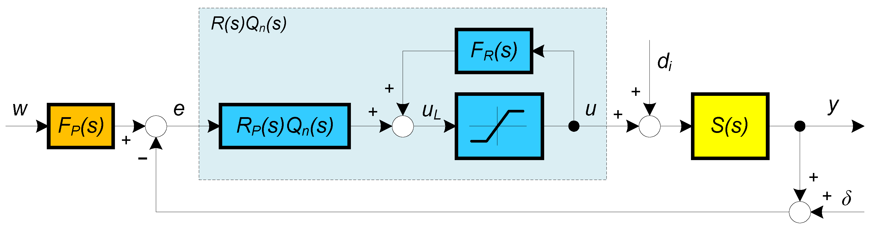
2.6. Basic Constrained Series MRDP-PIDA Modifications

In solving the MRDP optimal setting of constrained series PID controllers, it has been shown that the typical overshoots in the process output and input signals caused by the control constraints, can be eliminated. This is accomplished by selecting the smallest numerator time constant of the MRDP optimal controller transfer function as the time constant T i within the automatic reset filter (4) [27,39].
Contrary to popular belief, [39] has also shown that controllers based on simpler IPDT process models can perform better than controllers based on more complex first-order time-delayed (FOTD) models.
MRDP-optimal PID controller design can also be extended to constrained controllers with higher order derivatives [26,27,35]. However, for controllers with even derivatives (such as the PIDA controller), only approximate factorization can be performed by replacing complex numerator zeros with real ones. The aim of this article is to analyze in more detail the problem of approximating the complex zeros of the PIDA controller (started in [28]) and its impact on the obtained control performance. In addition, this article also investigates the limitations of the IPDT model in more complex time-delayed systems with dominant first-order dynamics and compares its performance with alternative design methods.
In [26], the optimal removal of overshoots in the case of constrained control was investigated using the performance portrait method. This was accomplished by examining the closed-loop responses for a grid of controller parameters using a “computer-aided trial-and-error method”. For a grid with a large number of PIDA controller parameters, the number of simulations required to obtain an estimate of the desired optimum was also very high. The number of trials required to obtain a relatively accurate optimal controller setting was over 10,000 [26].
From a practical point of view, this is very time consuming and it is better to find suboptimal tuning methods. Of course, these should be sufficiently accurate with a much smaller number of simulations. One possible approach is to modify the setup presented in [26,35], where the automatic reset time constant T i is chosen as the smallest time constant in the controller’s numerator. An attempt to generalize this approach to the PIDA controller encountered the problem of the complex conjugate controller numerator. Since the controller numerator (5) T A 2 s 2 + T D s + 1 = 0.0484 s 2 T d 2 + 0.4168 T d s + 1 gives the complex zeros
s 1 , 2 = ( 4.305785124 ± 1.456492874 j ) / T d = 4.5455 e ± j 0.3262 / T d ,
it does not allow us to assign the corresponding time constant to the automatic reset. However, neglecting the imaginary part, one obtains a double real pole s 1 , 2 = 4.305785124 / T d and the corresponding double real time constant T 2 < < T i = 2.5832 T d , enumerated as
T 2 = T d / 4.305785124 = 0.232 T d
Of course, we should remember that replacing a complex number with its real part (23) is only one possibility. Another way is to replace a complex number by its absolute value (module) s 1 , 2 = 4.5455 / T d . It would then be possible to deal with the corresponding double real time constant
T 2 = T d / 4.5455 = 0.22 T d
For the MRDP-PIDA controller parameters T i , K p , T D , T A 2 (15) and a new automatic reset time constant T ¯ i = T 2 , the new set of controller parameters specified as T ¯ i , K ¯ p , T ¯ D , T ¯ A 2 , or T ¯ i , K ¯ p , K ¯ d , K ¯ a , which nearly preserve the MRDP-optimal controller transfer function, can be calculated as follows:
K ¯ p = K p T 2 T i ; T ¯ D = T i + T 2 ; K ¯ d = K ¯ p T ¯ D ; T ¯ A 2 = T i T 2 ; K a = K ¯ p T ¯ A 2 ; T ¯ i = T 2 .
After replacing the numerator of controller (5) with T A 2 s 2 + T D s + 1 = 0.0484 s 2 T d 2 + 0.4168 T d s + 1 ( T 2 s + 1 ) 2 , the new controller parameters (denoted by overline) correspond to a new automatic reset time constant T ¯ i = T 2 . At the same time, the previously derived transfer function of the MRDP controller specified by parameters (15) was retained, as can be seen from the comparison of the corresponding parameters of the approximating and the new controller:
K P ( 1 + T 2 s ) 2 ( 1 + T i s ) T i s = = K ¯ P ( 1 + T 2 s ) ( 1 + T i s ) ( 1 + T 2 s ) T 2 s = K ¯ P ( 1 + T ¯ D s + T ¯ A 2 s 2 ) ( 1 + T ¯ i s ) T ¯ i s
The substitution of T 2 (23) and the MRDP parameters (15) yields a new set of parameters:
T ¯ i = 0.232 T d ; K ¯ p = 0.9323 0.232 2.5832 K s T d = 0.0837 K s T d ; T ¯ D = 2.815 T d ; K ¯ d = 0.236 K s ; T ¯ A 2 = 0.599 T d 2 ; K ¯ a = 0.0502 T d K s ;
By replacing the complex numerator zero (22) with its module (suggested by an anonymous reviewer) corresponding to the simpler numerical value τ 2 = 0.22 (24), we add the second possible “basic” set of controller parameters:
T ¯ i = 0.22 T d ; K ¯ p = 0.9323 0.22 2.5832 K s T d 0.0794 K s T d ; T ¯ D ( 0.22 + 2.58 ) T d = 2.8 T d ; K ¯ d = 0.2223 K s ; T ¯ A 2 = 0.22 2.5832 T d 2 0.568 T d 2 ; K ¯ a = 0.0451 T d K s ;
The contribution of the two modified controller settings (27) and (28) can be verified by simulation, but also by the circle criterion of absolute stability.

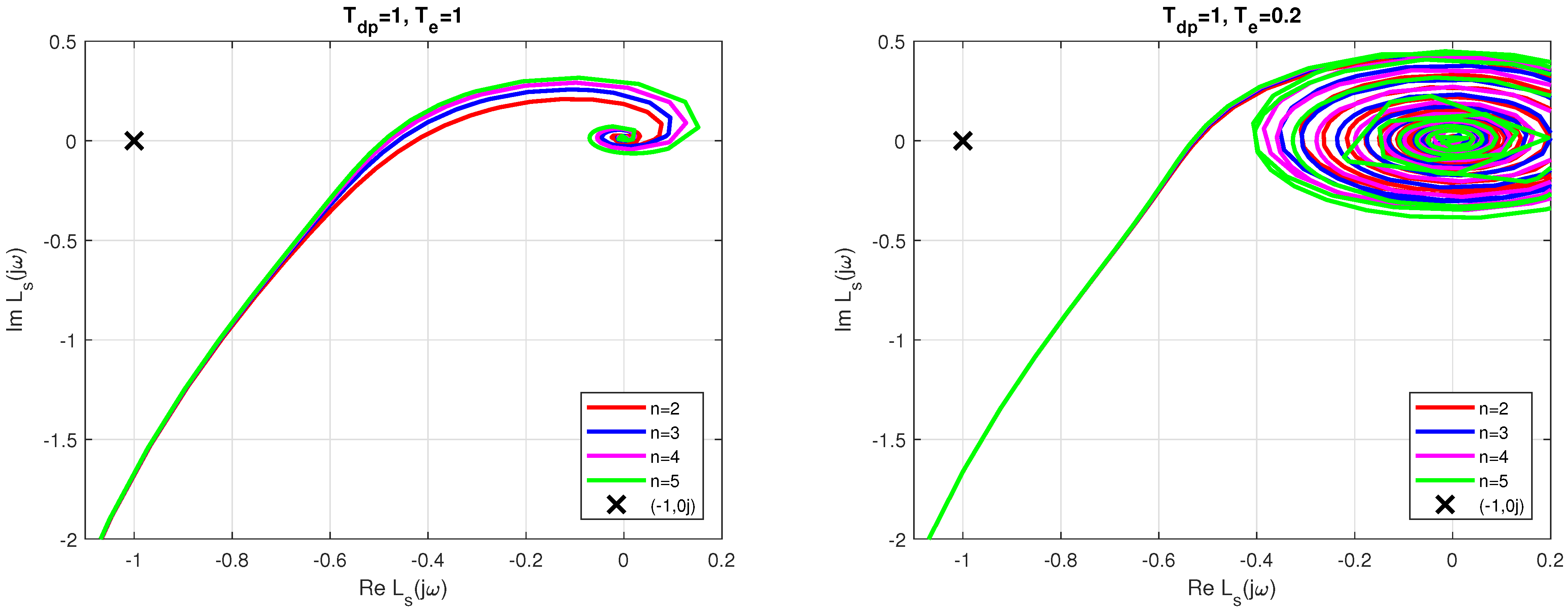
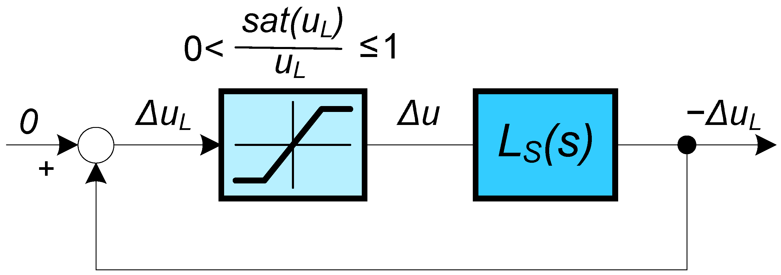
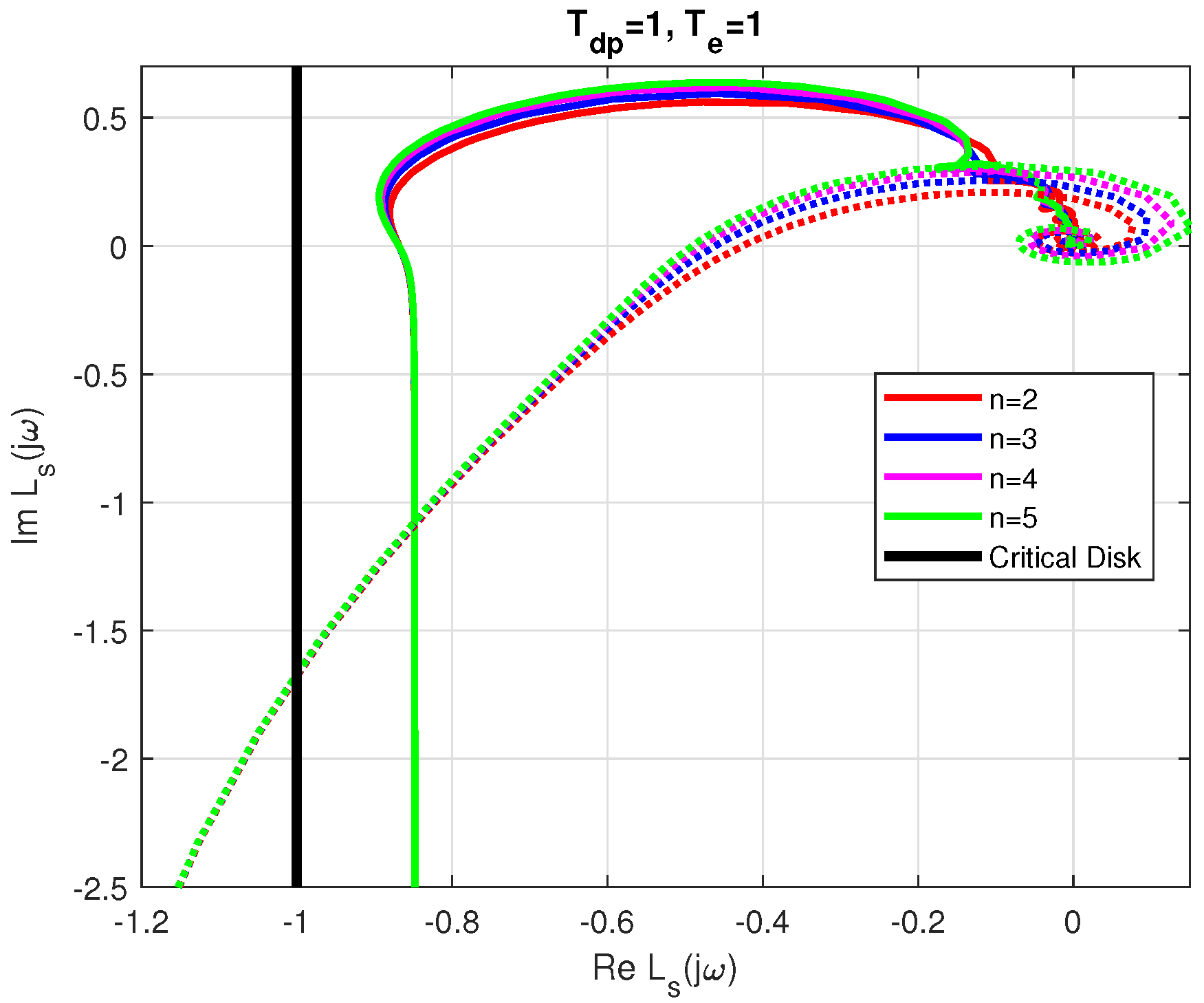
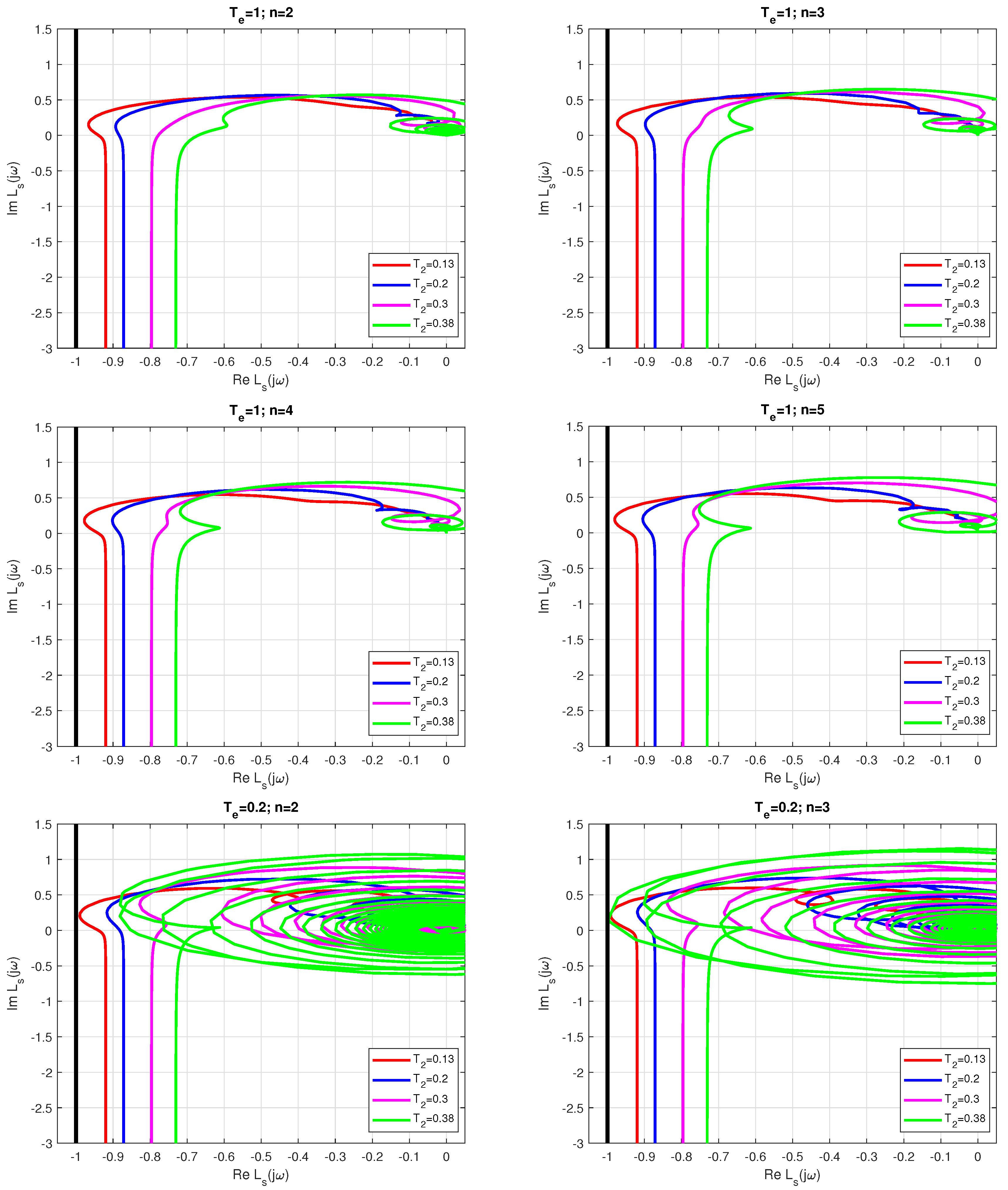
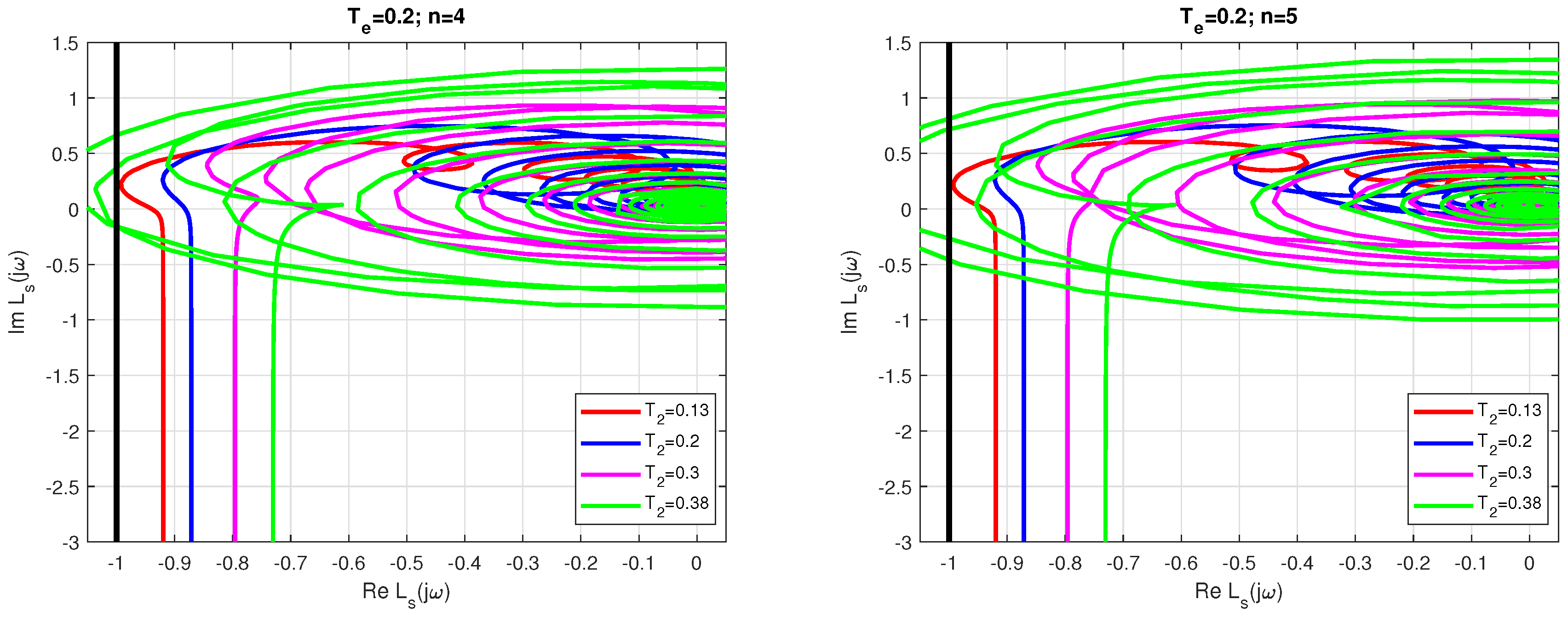
2.7. Absolute Stability Test

The saturation nonlinearity u = s a t ( u L ) represents a special case of the sector nonlinearity [ α , β ] , when for all u L holds α < s a t ( u L ) / u L β , where for large values u L α 0 and β = 1
0 < Δ u Δ u L 1
Thus, the critical circle intersecting the points ( 1 , 0 j ) and ( 1 / ϵ , 0 j ) and corresponding to the sector [ ϵ , 1 ] is projected for ϵ 0 onto the circle with an infinite radius as a vertical line passing through the point ( 1 , 0 j ) .
The circle criterion of absolute stability can be considered as a generalization of the Nyquist criterion for nonlinear time-varying circuits, which can be transformed into a sector nonlinearity and a linear part ([52,53,54,55,56], see Figure 4).
Definition 1 
(Absolute stability). Absolute stability (introduced by [57]) means that we can find c > 0 and δ > 0 such that any closed loop solution of the system x ( t ) satisfies the following relation of a monotonic decrease
| x ( t ) | c e δ t | x ( 0 ) | , t > 0
In other words, the envelope of the resulting solution x ( t ) is expected to have an exponential decay, typical for systems with dominant first-order dynamics with a time constant of 1 / δ . The circle criterion of absolute stability allows us to check the conditions for its fulfillment based on the position of the Nyquist curve with respect to the critical circle. In this case, the critical point ( 1 , 0 j ) of the Nyquist criterion is replaced by the critical circle, which has as its diameter the segment [ 1 / α , 1 / β ] on the real axis.
Considering series PIDA controller [26,27] with the filter Q n ( s ) (19), the PDA controller (3) and the positive feedback F R ( s ) = 1 / ( 1 + T i s ) (4) from the controller output, we obtain an equivalent linear system:
L s ( s ) = Δ u L Δ u = 1 1 + T i s R P ( s ) Q n ( s ) S ( s )
With respect to the critical point ( 1 , 0 j ) , the Nyquist curve of the MRDP-PIDA controller (15) in Figure 5 satisfies the stability condition in linear control. However, due to the presence of the saturation nonlinearity (which is a sector nonlinearity), the loop with the MRDP-PIDA controller does not satisfy the absolute stability requirement (30). This can lead to more complex responses with oscillations or even instability. On the other hand, the critical loop is not affected by the Nyquist curves of the modified PIDA controller with tuning in expression (27). Thus, satisfying the conditions of absolute stability for arbitrarily large u L when α 0 is in good agreement with the ideal shapes of the step responses obtained by simulation.
For the modified controller tuning (28), the corresponding Nyquist curves are almost unchanged.

2.8. Design of Prefilter

Since the one degree of freedom (1DoF) PIDA controller leads to setpoint step responses with high overshoots, a 2DoF controller can be designed by introducing a reference filter (prefilter) that removes the zeros from the F c ( s ) (13)
F P ( s ) = N p ( s ) D p ( s ) = b 3 s 3 + b 2 s 2 + b 1 s + 1 ( T A 2 s 2 + T D s + 1 ) ( T i s + 1 )
For constrained control, the simplest and most robust choice is to set:
b 3 = 0 ; b 2 = 0 ; b 1 = 0 ; N p ( s ) = 1
Following [58], accelerated setpoint step responses can be achieved by having the numerator of F P ( s ) cancel a closed loop time constant T o (14)
b 3 = 0 ; b 2 = 0 ; b 1 = T o = T d / 2 .

3. Problem Formulation

When setting up constrained series MRDP-PIDA controllers for IPDT models, the applied low-pass filter of the stabilizing controller and the setpoint prefilter must also be considered. The selected performance measures are used to evaluate transients with the optional T 2 parameter. In addition, the specified control constraints should allow the achievement and maintenance of a steady state for all constant inputs considered. To verify the effect of the control constraints, the evaluations should be repeated with different control limits, or the obtained simulation results should be analyzed with the circle criterion of absolute stability.
In this regard, the existence of two basic mappings of the complex controller zero into the real value motivated the study of the properties of the controller factorization considering a wider interval of T 2 values in [28]. In this work, this analysis is extended in terms of optimality by trying to improve the constrained performance of MRDP-PIDA by modifying the basic solutions, i.e., by choosing T 2 0.232 T d , or T 2 0.22 T d .

3.1. Effects of the Tuning Parameters on Absolute Stability

The first step in developing the parameterized constrained controller MRDP-PIDA with a free tuning parameter T 2 (25) is to test whether the constrained IPDT process is absolutely stable using controller tuning (25) for all values T e / T d p [ 0.2 , 1 ] (recommended for linear unconstrained control according to Proposition 1). The parameter τ 2 = T 2 / T d is thus extended to a wider range of values, including mappings of the complex controller numerator zero (23).
The canonical circuit in Figure 6, which consists of the linear part L s ( s ) (31) generated by the modified constrained MRDP-PIDA controller with tuning (25) and saturation nonlinearity from sector [ 0 , 1 ] , is absolutely stable at least for all τ 2 = T 2 / T d p [ 0.2 , 0.3 ] .
The absolute stability is graphically proven by the Nyquist curves in Figure 6, which for the given values lie to the right of the vertical line passing through the point ( 1 , 0 j ) representing the limiting case of the critical circle centered in ( , 0 j ) and radius R . For T e / T d p = 0.2 and T 2 / T d p = 0.13 , the Nyquist curve almost touches the critical circle. For T e / T d p = 0.2 and T 2 / T d p = 0.38 , the Nyquist curve already intersects the critical circle. This proves that a further increase in the value of T 2 / T d p is generally no longer useful.
At T e / T d p = 1 , of course, the safety margin increases. In this case, it would be possible to partially extend the range of usable values of T 2 (see Figure 7). It can also be shown that for higher values of T e / T d p , the area of absolute stability with respect to T 2 / T d p increases further.

3.2. Quantitative Evaluation of the Effects of the Tuning Parameters

The cost function for optimizing the controller with respect to the free tuning parameter can be based on the setpoint step responses:
J s = I A E s ,
disturbance step responses with the cost function
J d = I A E d ,
or on a combined cost function by selecting a trade-off between servo and regulatory control with m [ 0 , 1 ] :
J m = m I A E s I A E s , m i n + ( 1 m ) I A E d I A E d , m i n ; m [ 0 , 1 ] .
Here, I A E s , m i n and I A E d , m i n represent the minimum values that can be obtained under the shape-related constraints in the form
T V 0 ( y s ) ϵ y s ; T V 1 ( y d ) ϵ y d ; T V 1 ( u s ) ϵ u s ; T V 1 ( u d ) ϵ u d .
Remark 5 
(Acceptable deviations from ideal step responses). An optimal PIDA controller should guarantee the minimum of the chosen cost function J that is achievable under the given constraints on the shape-related deviations of the input and output variables (38).
Similarly, as stated in [44], the optimal PIDA performance should be defined by the tolerable deviations from ideal responses, ideally by
ϵ = ϵ y s = ϵ y d = ϵ u s = ϵ u d 0 .
The closed-loop responses with the linear MRDP-optimal PIDA controller (15) and (16) with the filter (19) tuned according to (20), where T e = n T f , and with a sufficiently long T e (e.g., T e T d p ), seem to satisfy the requirements. To verify the closed-loop properties in the constrained case, a simulation is usually used. However, due to the limited precision of computer simulations, some “sufficiently” small positive limits should be chosen instead. For example, to allow multiple control pulses at the output of the controller, its allowable deviations should be chosen proportionally higher than at the process output, e.g., according to
ϵ y = ϵ y s = ϵ y d = 0.001 ; ϵ u = ϵ u s = ϵ u d = 10 ϵ y = 0.01
Obviously, this“ad hoc” choice has a significant impact on the resulting performance, but it represents a compromise between performance in practice and computational cost and does not preclude additional refinements by choosing other relevant limits. For practical purposes, the looser requirements for allowable shape deviations
ϵ y = ϵ y s = ϵ y d = 0.004 ; ϵ u = ϵ u s = ϵ u d = 10 ϵ y = 0.04
can also be tested.
Note that the above weakening of the control signal shapes requirements can provide additional degrees of freedom in optimizing higher order controller modes. This is similar to the weakening of the absolute stability requirements (30).

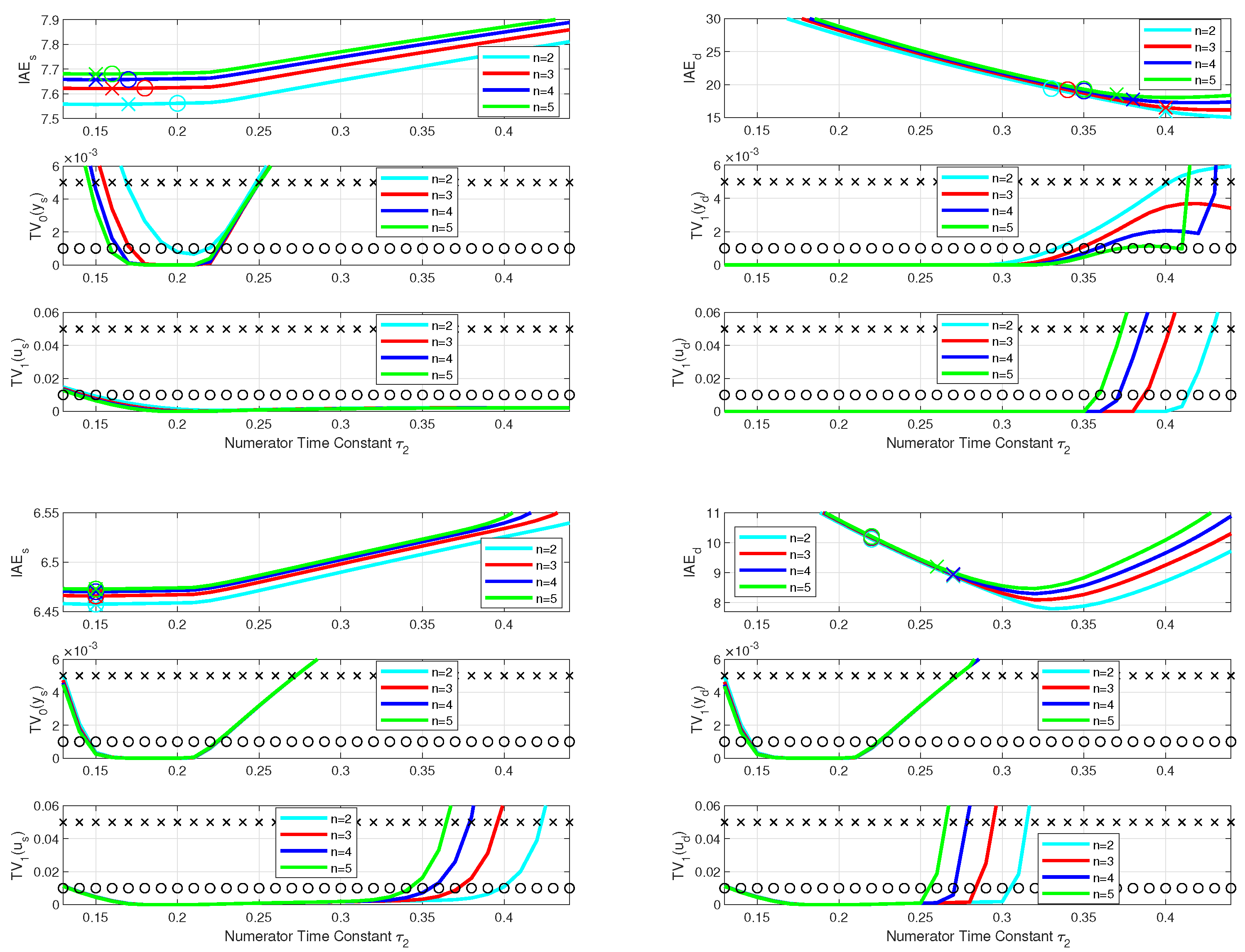
3.3. One-Dimensional Performance Test

Here, we will analyze the effects of the free parameter T 2 in (25) and determine the range of its allowable values under constraints. The deviations at the plant input and output are defined by the performance limits (40) and (41), for n [ 2 , 5 ] , T f = T e / n and T e / T d p [ 0.2 , 1.0 ] , T d p = 1 , K s p = 1 . We will also test the difference between the realizations (23) and (24).
The analysis of the influence of the tuning parameter τ 2 = T 2 / T d is an extension of the original study from [28]. By considering a wider range of filters and performance measures, it shows several new results. The first extension is defined by the range of the dimensionless parameter
τ 2 = T 2 / T d [ 0.13 , 0.44 ] ; Δ τ 2 = 0.01
Any evaluation of the setpoint and input disturbance step responses corresponding to some values τ 2 requires appropriate controller transfer functions with R P ( s ) extended by a filter Q n ( s ) , n 2 . Since the filter of the controller suppresses the measurement noise, four different values of n [ 2 , 5 ] are considered in the analysis. However, to determine the influence of the filters on the closed-loop response, the analysis is initially performed without the measurement noise.
The benefits of the modified setting become apparent only when the control signal saturates. In order to study the responses under different constraints, the limits for the setpoint step responses are set:
U m a x = 0.1 , U m i n = 0.1
selected separately from the limits for the response to input disturbance:
U m a x = 0.1 , U m i n = 1.1
This choice makes it possible to obtain stable steady states with a sufficient control signal span before and after the transients.

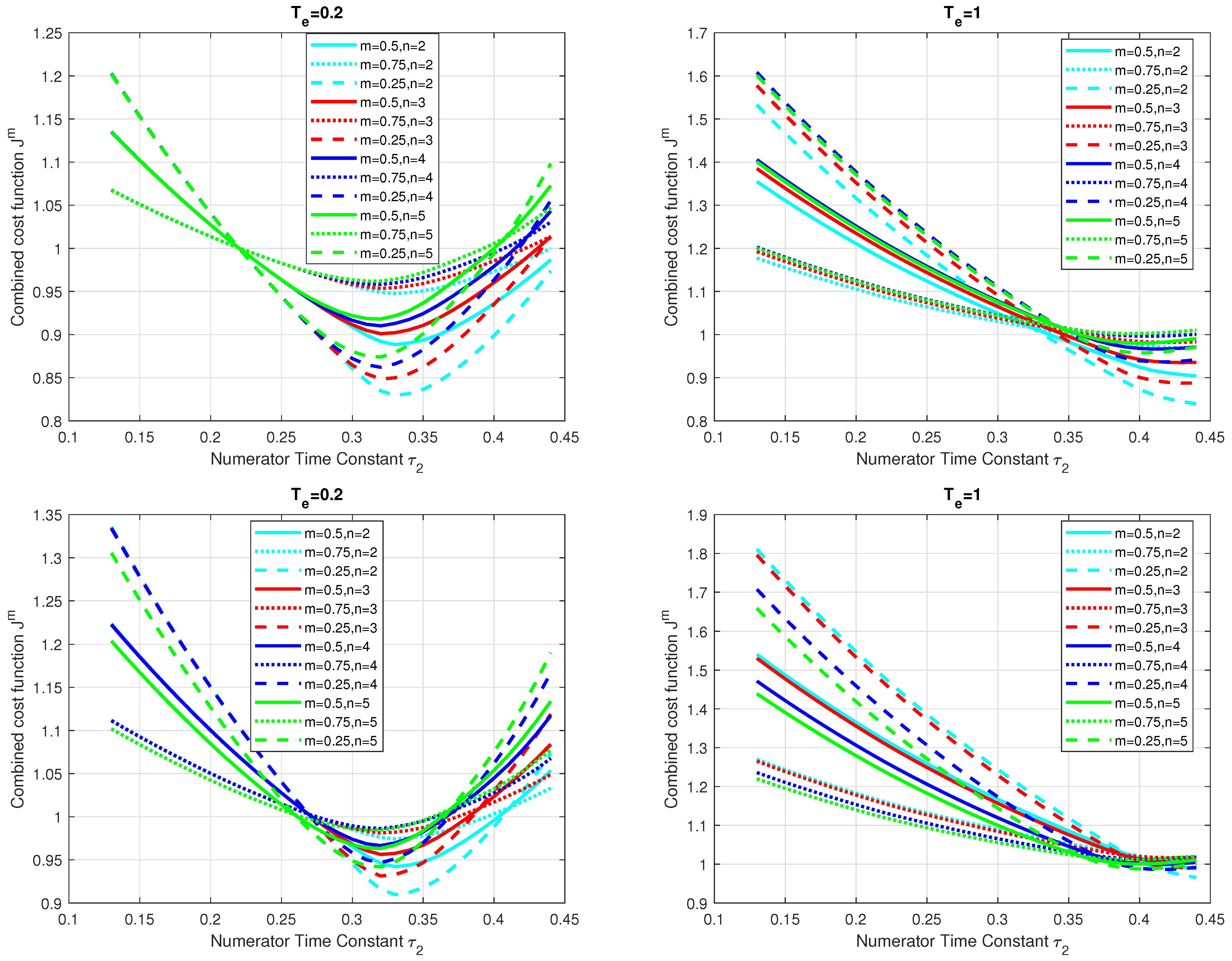
3.4. Evaluation of the Controller Tuning

The choice of the equivalent delay of the filter T e and the time constant T 2 leads to a set of tuning pairs that can be used to set the appropriate closed loop dynamics. To reduce the number of experiments, we will use a relatively aggressive controller with T e / T d p = 0.2 and a“softer” controller with T e / T d p = 1 . This second setting will be referred to as the “default” in the following text.
The effects of the tuning parameter τ 2 = T 2 / T d p on the cost functions (35)–(37) for the allowable shape deviations defined by (40) and (41) are shown in Figure 7 and Figure 8.
By reducing T e , it was possible to reduce both I A E values: I A E s (from about 7.6 to 6.46) and even more I A E d (from 20 to 10). Reducing T e not only improves I A E values, but also allows specified shape deviations with lower τ 2 values.
For T e = 1 and ϵ y = 0.001 , the allowable shape deviations of the target responses (depending on n) for τ 2 are achieved in the range of 0.16–0.20 and up to 0.23. For the disturbance responses, the allowable range is 0.13–0.33. For ϵ y = 0.004 , the τ 2 intervals corresponding to the allowable shape deviations increase to 0.15–0.25 for the setpoint responses. For the disturbance responses, the allowable range is 0.13–0.37 and up to 0.4.
For T e / T d p = 0.2 and ϵ y = 0.001 , the allowable shape deviations of the setpoint responses (depending on n) for τ 2 are reached between 0.15–0.23. For the disturbance responses, the allowable range is 0.13–0.22. For ϵ y = 0.004 , τ 2 increases to 0.15–0.27 for the setpoint responses and to 0.13–0.27 and up to 0.28 for the disturbance responses, corresponding to the allowable shape deviations.
Using the combined cost function (37) under the allowable constraints (40) and (41) shows that it is possible to increase the value of τ 2 by about 50% (to τ 2 0.3 ) from the values recommended for the setpoint step responses, while the slope of the reduction increases as the weighting coefficient m is reduced. Such modification of the controller corresponds to improved disturbance rejection performance. Therefore, taking into account the simplest possible numerical parameters, the following proposition can be formulated.
Proposition 2 
(Recommended numerator time constant of the controller τ 2 = T 2 / T d p ). “MRDP-optimal” values for the setpoint step responses are τ 2 = 0.232 (23), or τ 2 = 0.22 (24)–(28). The values increased by 50% ( τ 2 = 0.348 and τ 2 = 0.33 , respectively) can be recommended as“near optimal” for the disturbance step responses.
Based on experiments, the recommended values could be even simpler: τ 2 = T 2 / T d p = 0.2 for the near-optimal tracking response and τ 2 = 0.3 for the near-optimal disturbance rejection response.
The above approximations were obtained by evaluating the simulations with “smooth” T e = T d p (20) and “aggressive” T e = T d p / 5 . For the setpoint responses (see Figure 7, top left), the lowest values of the I A E s from the experiments agree well with the values corresponding to the controller zero approximations using the module approach (24).
For T V 0 ( y s ) , it would be more accurate to consider τ 2 0.232 (23) for n = 2 , but to make it easier to remember, we can choose τ 2 = 0.22 as the (optimal) default value. This is also suitable for a much more aggressive controller setting given by the filtering parameter T e = T d p / 5 (Figure 7, bottom left). Since the experimentally determined optimal I A E s values lie in the flat part of the measured dependencies, we can simply choose the default value τ 2 = 0.2 .
For disturbance suppression, the I A E d value decreases as soon as τ 2 increases sufficiently (depending on T e ). For the smoother setting with T e = T d p , the optimal values are τ 2 > 0.35 , but for a more aggressive setting of T e , the default value of τ 2 = 0.33 can be chosen. This is 1.5 times the value recommended by the optimal setpoint responses (see Figure 7, right). Therefore,
τ 2 = 0.2 * 1.5 = 0.3
can be recommended as a simplified default setting.
Proposition 3 
(Three sets of recommended PIDA controller settings). Settings (27) and (28) are denoted by the symbols PIDA w 0 , or PIDA w m , respectively. They ensure near-minimum values of the I A E s for the setpoint step responses, with allowable deviations from the ideal shapes of the input and output process signals. The setting corresponding to the numerically simplest value τ 2 = 0.2 can be calculated as follows:
T ¯ i = 0.2 T d ; K ¯ p = 0.0722 K s T d ; T ¯ D = 2.7832 T d ; K ¯ d = 0.2009 K s ; T ¯ A 2 = 0.5166 T d 2 ; K ¯ a = 0.0373 T d K s ;
For the disturbance responses, the recommended settings when increasing the value of τ 2 (23) by a factor of 1.5 are as follows:
T ¯ i = 0.348 T d ; K ¯ p = 0.126 K s T d ; T ¯ D = 2.931 T d ; K ¯ d = 0.368 K s ; T ¯ A 2 = 0.899 T d 2 ; K ¯ a = 0.113 T d K s ;
and are indicated by the symbol PIDA d 0 . The abbreviation PIDA d m can be used for modified settings based on (24) and corresponding to the following values:
T ¯ i = 0.33 T d ; K ¯ p 0.1191 K s T d ; T ¯ D = 2.91 T d ; K ¯ d = 0.3466 K s ; T ¯ A 2 = 0.8525 T d 2 ; K ¯ a = 0.1015 T d K s ;
Finally, the simplified setting that complements PIDA w , specified by (45)
T ¯ i = 0.3 T d ; K ¯ p = 0.1083 K s T d ; T ¯ D = 2.8832 T d ; K ¯ d = 0.3122 K s ; T ¯ A 2 = 0.7750 T d 2 ; K ¯ a = 0.0839 T d K s
can be designated as PIDA d .
It is obvious that the controller tuning PIDA d 0 , PIDA d m and PIDA d result in a “tighter” control with a more noisy controller output than PIDA w 0 , PIDA w m and PIDA w . Similarly, a pair of settings based on approximating the complex zero by its real part will result in slightly tighter control than when replaced by the modulus. Of course, the parameter τ 2 [ 0.2 , 0.33 ] can still be considered as a free tuning parameter, used to modify the overall dynamics of the closed loop in terms of the trade-off between servo and control [44,59,60,61,62,63].

4. SIMC Controller Design

The first method for setting controllers with automatic reset and derivative terms was published shortly after hyper-reset controllers were introduced to the market [64]. In the following decades, a large number of different “optimal” methods have been proposed for the design of both controllers with automatic reset and PID controllers with parallel integral action. O’Dwyer attempted to summarize these efforts in his publication [42], but since many more have been added recently, it is not possible to compare even the most basic approaches. Since this paper focuses on the design of constrained series PIDA controllers for IPDT models, the new approach will be compared with the SIMC method. When the SIMC method was developed, it had the ambition to become “probably the best simple PID tuning rules in the world” [31,65]. The motivation to choose this approach is due to some similarities with the proposed approach. The SIMC method is also based on the required first-order closed-loop dynamics, it deals with the design of series PIDs (i.e., with automatic reset), and its results have already been compared with several other well-known control design methods, which further increases the impact of the obtained evaluation. Last but not least, we wanted to ensure that the proposed methodology successfully improves the dead-time approximation. Therefore, it can be an alternative for building a modular approach that allows the gradual increase in the controller order and its efficiency.

4.1. Simplified Process Modeling

This last expectation may not be obvious, because the method incorporates several aspects of process modeling and performance evaluation to simplify calculations. The application to higher order process transfer functions begins with a reduction in process order by applying the so-called “half-rule” method. In the simplest case, a first-order time-delayed transfer function (FOTD)
F 1 ( s ) = Y ( s ) U ( s ) = K e T d s 1 + T 1 s
is achieved. It consists of the largest original process time constant in the denominator. The second largest neglected time constant in the denominator of the original process transfer function is partially added to the original process time delay (if any) and to the already mentioned largest time constant equally. Any shorter time constants in the original process denominator are added exclusively to the time delay by increasing it to a new estimate of T d .
To obtain the FOTD model (50), the zeros of the original process can also be substituted. For example, for a stable process with zero
P ( s ) = 2 15 s + 1 ( 20 s + 1 ) ( 1 s + 1 ) ( 0.1 s + 1 ) 2
according to ( 15 s + 1 ) / ( 20 s + 1 ) 3 / 4 and the half rule, [31] gives the FOTD model
F 1 ( s ) = 1.5 e 0.15 s 1.05 s + 1 .
F 1 ( s ) (52) is preferably used for the design of series PI controller.
The series PID controller usually starts with the transfer function of the second-order time-delay (SOTD) model
F 2 ( s ) = Y ( s ) U ( s ) = K e T d s ( 1 + T 1 s ) ( 1 + T 2 s ) .
The reduction of the denominator of the process begins by dividing the third largest time constant and adding it to the second largest original constant and to the time delay in equal parts. For the process (51), this results in
F 2 ( s ) = 1.5 e 0.05 s ( s + 1 ) ( 0.15 s + 1 ) .
By generalizing the above procedures, the series PIDA series controller can begin with the third-order time-delay (TOTD) model transfer function
F 3 ( s ) = Y ( s ) U ( s ) = K e T d s ( 1 + T 1 s ) ( 1 + T 2 s ) ( 1 + T 3 s ) .
For (51), for example, one could obtain a simplified third-order model:
F 3 ( s ) = 1.5 ( s + 1 ) ( 0.1 s + 1 ) 2 .

4.2. Design of the SIMC Controller

The next step following the SIMC method is to define the desired closed loop transfer function. To minimize the number of optional parameters, a simple FOTD model with the time constant T c l was chosen:
F c l ( s ) = Y ( s ) W ( s ) = 1 1 + T c l s e T d s .
While the process time delay T d is usually unavoidable and therefore kept the same as in the process, the time constant T c l can be used as a tuning parameter. The exponential term of the pure time delay in the controller
R ( s ) = F c l ( s ) ( 1 F c l ( s ) ) F ( s )
can be approximated with different approaches. It is therefore possible to obtain different types of controllers.
In the simplest case, the first-order Taylor series expansion according to
e T d s 1 T d s
results into the series proportional-integral (PI) controller:
1 R 1 ( s ) = U ( s ) E ( s ) = 1 + T 1 s K ( T c l + T d ) s = K c ( 1 + 1 T i s ) , T i = T 1 > 0 ; K c = T 1 K ( T c l + T d ) .
In the controller form with automatic reset, it is implemented with a gain C 1 ( s ) = K c and with a feedback filter
F A R ( s ) = 1 1 + T i s .
The first-order Padé approximation of the dead-time term with:
e T d s 1 s T d / 2 1 + s T d / 2
yields a PID controller transfer function:
1 R 2 ( s ) = K c 1 + 1 T i s 1 + T D s 1 + T f 1 s , T i = T 1 ; T D = T d / 2 ; K c = T 1 K ( T c l + T d ) ; T f 1 = T c l T d 2 ( T c l + T d ) ,
which consists of a filtered PD controller C 2 ( s ) = K c ( 1 + T D s ) / ( 1 + T f 1 s ) and is augmented by an automatic reset (61) that modifies its output.
Similarly, the second-order Padé approximation
e T d s 1 T d / 2 s + T d 2 s 2 / 12 1 + T d / 2 s + T d 2 s 2 / 12
results into the proportional–integral–derivative–acceleration (PIDA) controller [45]
1 R 3 ( s ) = K c 1 + 1 T i s 1 + T D 1 s + T D 2 s 2 1 + T f 1 s + T f 2 s 2 ; T D 1 = T d 2 ; T D 2 = T d 2 12 ; T = T c l + T d ; T i = T 1 ; K c = T 1 K T ; T f 1 = T c l T d 2 T ; T f 2 = 0.0833 T c l T d 2 T .
It may consist of a PDA controller C 3 ( s ) = K c ( 1 + T D 1 s + T D 2 s 2 ) / ( 1 + T f 1 s + T f 2 s 2 ) and an automatic reset (61) with a positive feedback loop.
Remark 6 
(Basic SIMC constraint). Note that the model-based design (58), which is based on the cancellation of the process transfer function F ( s ) , is applicable only to stable models. Therefore, the SIMC method [31] has been significantly improved in practice by an ad hoc requirement of a double real dominant pole of a delay-free loop. In this way, the applicability of the method could be extended at least for integrating process models. Such models can also be interpreted as a limiting case of systems with a long dominant time constant, if, e.g.,
S 1 ( s ) = Y ( s ) U ( s ) = K / T 1 e T d s s + 1 / T 1 K s e T d s s .
The application to IPDT models proposed in [31] for a delay-free process (8) ( T d = 0 ) leads to a double real dominant pole of the closed loop with
T i = 4 / ( K s K c ) ; K c = 1 / ( 2 K s T c l )
For a nominal process (8) with T d > 0 and T c l = T d in (57), expressions (66), (67) and (60) yield a simple SIMC tuning
K c = 1 / ( 2 K s T d ) ; T i = 8 T d
To further demonstrate the impact of the choice of T c l , we also consider T c l = T d / 2 , which leads to the following results:
K c = 2 / ( 3 K s T d ) ; T i = 6 T d

4.3. SIMC Design for Higher-Order Models

In attempting to generalize SIMC design [31] for higher order process models, we encounter several unsystematic steps in [31]. This complicates the application and generalization of the solutions already proposed [45].
  • The first-order transfer function requirement (57) for the second-order plant models (53) in [31] leads to an improper controller that is not feasible in practice.
  • The actual controller design for second-order processes (53), with a minimum number of optional parameters, can be implemented [45] by choosing
    2 F c l ( s ) = 1 ( 1 + T c 2 s ) 2 e T d s .
  • Once the desired closed-loop transfer function (57) has been chosen, the filter time constant T f , which is required to implement the controller, should be systematically added to the process model using the aforementioned half-rule. Instead, the implementation of a series PID controller with an additional first order filter T f = T D / 100 was proposed in [31]
    U ( s ) = K c T i s + 1 T i s W ( s ) T D s + 1 T f s + 1 Y ( s )
    The author admitted that in practice (especially for noisy processes) larger values of T f [ T D / 10 , T D / 5 ] have to be used. However, it is not clear why the filter was not systematically included in the design using the half rule. Indeed, the design of the controller without considering T f is not accurate, especially if you use a higher-order filter to reduce the noise level.
  • The controller design is based on the setpoint response requirements, so the performance of disturbance responses can only be considered indirectly.
  • The SIMC design does not address possible control signal (or state) constraints.
  • As pointed out in [45] and in Remark 5, when higher order models are used, adjustments to the performance measures are required. The use of total variation proposed in [31] penalizes control responses with multiple control intervals, which are required in higher order process models.
For a consistent comparison of the proposed MRDP-PIDA with the SIMC design, several aspects in the SIMC approach need to be changed or added. Therefore, it is more appropriate to rename it as the comparison with the SIMC-inspired design. There are several ways to achieve the necessary generalizations when higher order process models are used. Here, the modifications that require minimal changes to the original design are preferred, e.g., using the required closed-loop transfer function (57) for higher-order process models as well, with the aim to obtain the dominant first-order dynamics. In addition, the filters required to achieve feasible controller transfer functions will already be included in the process model and the setpoint prefilters will also be used.
For the second-order plant models (53) and the dead time approximated by Taylor, [31] derived the second type of series PID controller
2 R 2 ( s ) = K c 1 + 1 T i s 1 + T D s ( 1 + T f s ) n ; T i = T 1 ; T D = T 2 ; K c = T 1 K ( T c l + T d ) ; n 1 .
By using the first-order Padé approximation (62), it might be possible to derive the second type of PIDA controllers.
2 R 3 ( s ) = K c 1 + 1 T i s ( 1 + T D 1 ) ( 1 + T D 2 s ) ( 1 + T f 1 s ) ( 1 + T f s ) n ; T i = T 1 ; T D 1 = T 2 ; T D 2 = T d 2 ; T f 1 = T c l T d 2 ( T c l + T d ) ; K c = T 1 K ( T c l + T d ) ; n 1 .
In both cases, the n-tuple filter time constant T f must be included in the process model (53), according to the half-life rule.
Similarly, for the third-order plant models (55), one could derive the third type of PIDA controller
3 R 3 ( s ) = K c 1 + 1 T i s ( 1 + T D 1 s ) ( 1 + T D 2 s ) ( 1 + T f s ) n , T i = T 1 ; T D 1 = T 2 ; T D 2 = T 3 ; K c = T 1 K ( T c l + T d ) ; n 2 .
together with the inclusion of the n-tuple filter time constant T f in the process model (55).
For the processes with a long time constant T 1 and for integrating processes, a modification can also be derived along the lines of (66), (67) and (60).

4.4. Prefilter in SIMC Design

In [31], no prefilter F P ( s ) is considered to remove the zeros from the F c ( s ) (such as (32)) necessary to eliminate overshoot. However, such a prefilter can always be added with a denominator equal to the controller used and a numerator equal to N p ( s ) = 1 . The use of the controller (71) avoids the differentiation of the setpoint signal and represents another possible alternative to eliminate the initial control overshoots in setpoint step responses.

5. IPDT System Control

A brief comparison of the responses of SIMC-PI and the entire family of series-automatic based controllers with derivative degree m [ 0 , 5 ] was discussed in [27]. The comparison is now extended with modified MRDP-based constrained series PIDA w 0 and PIDA d 0 controllers and with SIMC-based PI, PID, and PIDA controllers derived for an IPDT model (denoted 1 R 1 , 1 R 2 and 1 R 3 , respectively). For the setpoint and disturbance step responses, the control signal constraints were chosen differently to allow the final steady states to be reached. Of the three options recommended in Proposition 3, the most aggressive controller setting (PIDA w 0 and PIDA d 0 ) was chosen to highlight the differences between the compared methods.

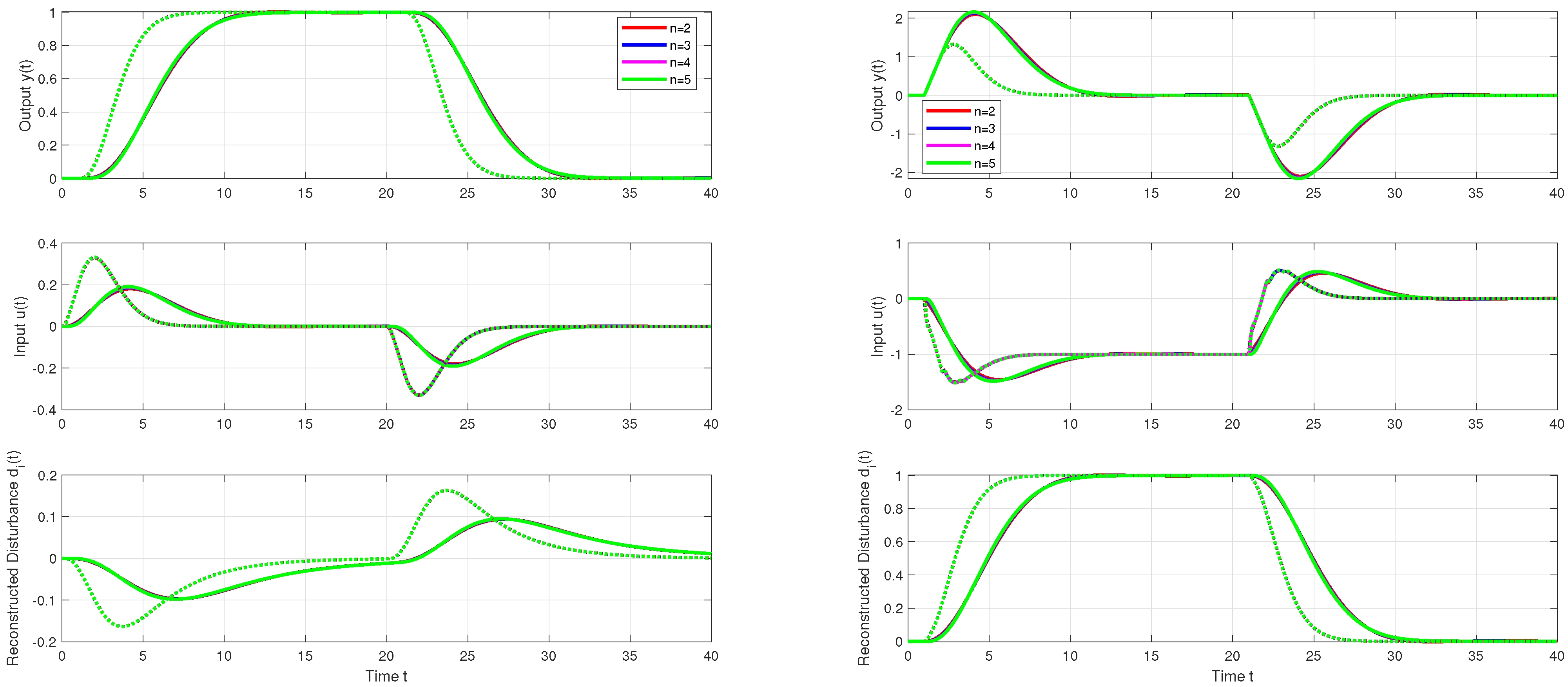
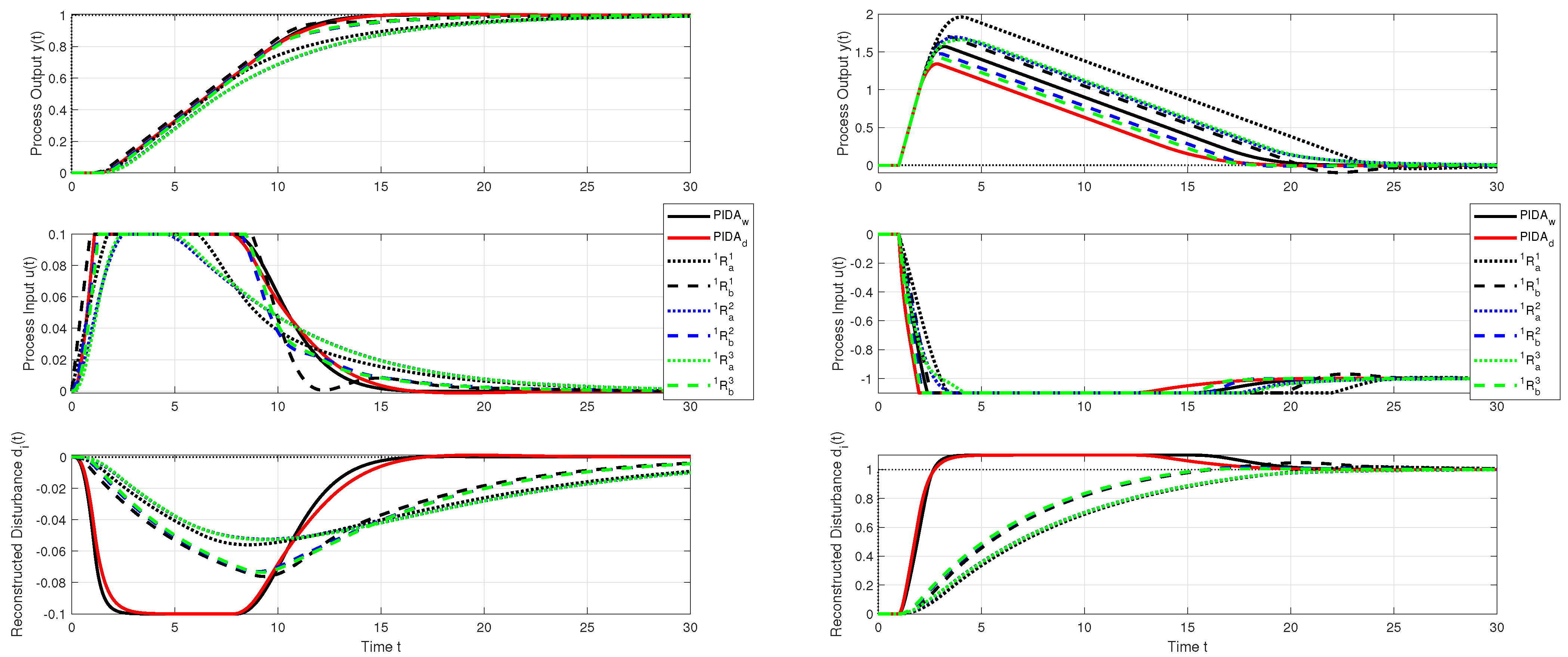
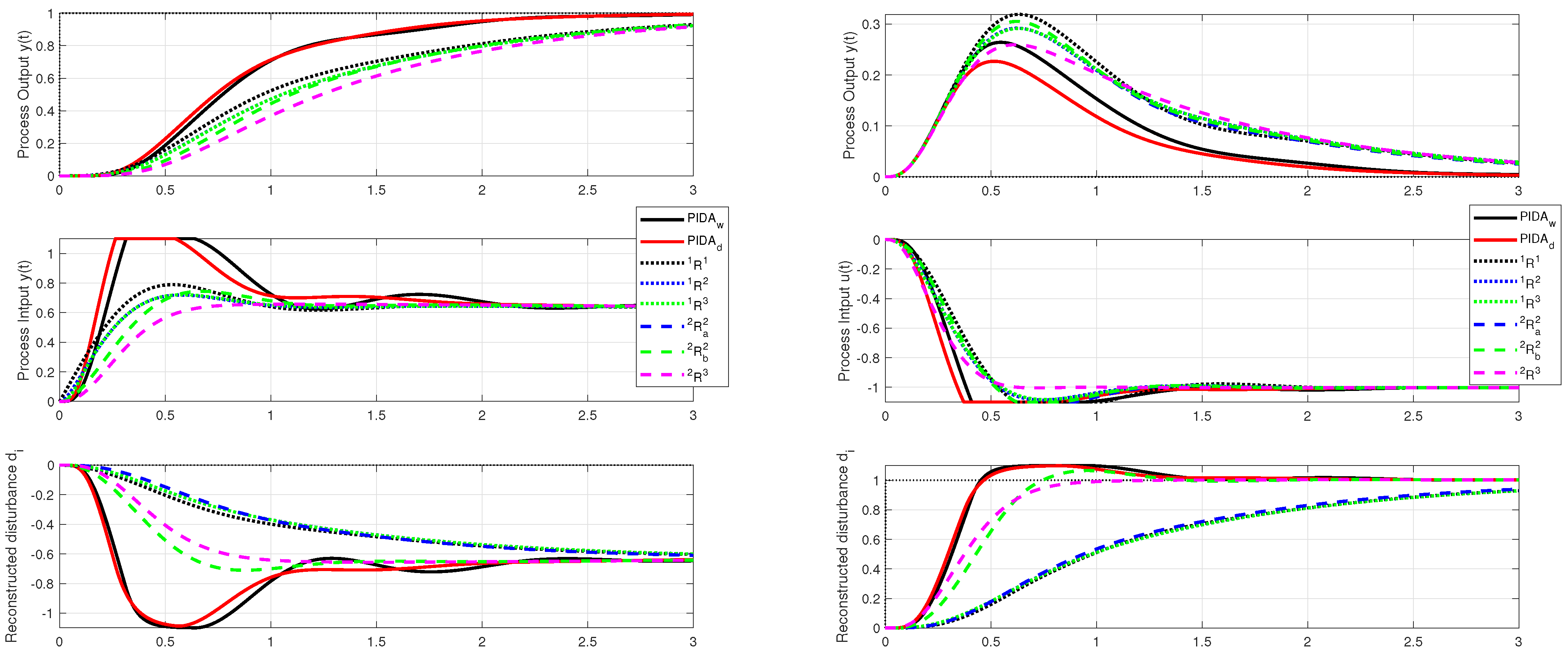
5.1. Setpoint and Disturbance Responses without Measurement Noise

As can be seen in Figure 9, the setpoint step responses of the PIDA w 0 and PIDA d 0 controllers (index 0 omitted for simplicity) for the IPDT process are almost indistinguishable. However, PIDA d 0 has a much better disturbance rejection response. The advantages of the MRDP design are most evident in the higher speed of disturbance reconstruction in the setpoint step responses.
As shown by the setpoint step responses of the SIMC controllers (Figure 9) with T c l = T d , the use of higher order dead time approximations in 1 R 2 and 1 R 3 does not yield significant improvements compared to the 1 R 1 controller. A partial improvement was achieved in the disturbance rejection by 1 R 2 and 1 R 3 . The advantages of using the 1 R 2 and 1 R 3 SIMC-PID and PIDA controllers become more apparent when faster closed-loop responses with T c l = T d / 2 (dashed responses) are selected. In such cases, however, the PI controller shows a slight overshoot.
It has already been stated in [27] that “the SIMC-PI controller derived using ad hoc assumptions for the IPDT model gives quite good results”. We can also agree with [31] that the choice of a double real pole in the closed loop in the original model-based approach for a delay-free system is one of the main advantages of the SIMC approach compared to IMC.

5.2. Measurement Noise Generated by the Uniform Random Number Noise Generator

In Matlab/Simulink, the measurement noise was generated by the Uniform Random Number block with sampling period T s = 0.001 and amplitude Δ n = 0.01 . To improve signal filtering, the equivalent filter time constant was increased to T e = 1 . The shapes of the responses are similar to those without noise, except that the control signals are covered by noise (in some cases it is very high). Therefore, the responses in Table 1 and Table 2 are interpreted quantitatively.
The fastest control speed for setpoint step changes (low I A E s ) is achieved with the 1 R b 1 controller with T c l = T d / 2 . However, the advantage of a simple PI-controller structure (which does not use filtering) is lost due to the presence of measurement noise (high T V 1 ( u ) value). Disturbance rejection is most optimal with PIDA d 0 (with the lowest value of maximum deviation) at the cost of high excessive control effort. However, using the combined cost function (12) can give you the freedom to choose the optimal solution. If you use the cost function J 1 with a relatively low weight for I A E , the optimum depends mainly on T V 1 ( u ) . If you use a relatively high weight for I A E ( J 10 ), the optimum depends mainly on I A E , which (for the disturbance responses) also correlates with lower values of m a x ( | e | ) .
Thus, the conclusion is that although the constrained PIDA w 0 and PIDA d 0 controllers give optimal performance in some cases, their design is more complex. Since, in this paper, only the modification with derivative degree m = 2 and a specific configuration of the implementation filter ( n = 4 , T e = 1 , T f = T e / n ) is addressed, the real impact of the proposed innovation will only become clear after a more comprehensive evaluation of the capabilities of the new modular system. This will allow us to choose the most appropriate solution for each practical situation, whereby the simplest alternatives will not be excluded.
Therefore, we proceed with the robustness test of the two new PIDA modifications and a comparative SIMC control created by controlling a stable process (51) considered in [31,66].

6. Stable Process Control

The SIMC design in [31] was illustrated using a transfer function (51) with significantly different time constants. Obtaining such a model with sufficient accuracy from real experiments is difficult. Moreover, such an approach is also questionable due to the simplifications of the obtained process model in the next stage. Finally, it leads to models (52), (54), or (56), which still need to be modified due to the controller filter required for the physical implementation and noise attenuation.

6.1. Step Response Based Approximation of Stable Process by IPDT Model

For the design of MRDP-PIDA, the IPDT model (8) of the process (51) can be obtained from its open-loop step response by generalizing the method of Ziegler and Nichols [35,39,67]. The original approach of Ziegler and Nichols uses the tangent line passing through the inflection point of the measured process response. However, due to the poor numerical properties of such an approach and the robust stability analysis in [43], the following approximation
F ( s ) = 1.01 e 0.12 s
is used in [29]. It successively approximates segments of the measured step response of different lengths by the IPDT model using the least squares method. Finally, following [43], the solution with the maximum possible value of the parameter K s was chosen.

6.2. Setpoint and Disturbance Responses—No Noise

An overview of the compared controllers can be found in Figure 10.
When setting the PIDA w 0 and PIDA d 0 controllers, the values n = 4 and T f = T e / n were again chosen, where T e = T d p = 0.12 corresponds to the IPDT model (75). The SIMC PI, PID and PIDA controllers labeled 1 R 1 , 1 R 2 and 1 R 3 are based on the FOTD transfer function (52) with T c l = 0.75 T d p , where T d p = 0.15 . Other types of PID and PIDA controllers labeled 2 R 2 and 2 R 3 then correspond to the SOTD model (54). They use T c l = 0.5 T d p , where T d p = 0.05 + T e . T e = T f = 0.12 is used to set the controller filter to the same equivalent delay as the PIDA w 0 and PIDA d 0 controllers. Controllers 2 R a 2 and 2 R b 2 have mutually exchanged the numerical values of model time constants T 1 and T 2 .
Although the adjustment of the PIDA d 0 controller was obtained to optimize the disturbance responses of the IPDT system, the higher robustness of this solution in controlling a stable system with internal feedback acting as a disturbance is reflected in Table 3 by a lower value of I A E s . However, smaller gains of the PIDA w 0 controller are reflected in a lower value of the excessive controller effort T V 1 u , which finally leads to the lowest value of J 1 for this controller. At the same time, the PIDA w 0 controller also has the highest T V 0 y value, which is due to a very low overshoot (less than 0.0072 / 2 ). Thanks to the higher robustness of the PIDA d 0 controller, its maximum output deviation is lower. However, it should be noted that these overshoots are much lower than the amplitude of the measurement noise Δ n = 0.01 . The noise of the controller is completely smoothed at the output thanks to the filtering properties of the process. However, as you can see from the T V 1 u values, the noise at the controller output can be quite high for some controllers. It is also worth noting that controllers 2 R b 2 and 2 R 3 provide the fastest reconstruction of the equivalent disturbance. The reconstructed disturbance at steady state is different from zero for all tested setpoint step responses, although the actual disturbance is zero. This happens because the reconstruction of a disturbance from the steady states is based on integrating models, even though the controller design is based on a stable process model [37].
Some relatively small overshoots are also detected by the T V 1 y values for disturbance responses with PIDA y 0 and PIDA d 0 controllers (see Table 4). PIDA d 0 also provides the minimum value of I A E , m a x ( | e | ) and J 10 for disturbance responses. However, PIDA d 0 is slightly more noisy than the PIDA y 0 controller. The latter provides the lowest values for T V 1 u and J 1 . Again, the 2 R 3 controller provides the fastest reconstruction of the equivalent disturbance.

7. Discussion of the Results Obtained

In terms of a more complex design, the advantages of the new MRDP-based constrained PIDA modifications do not seem entirely obvious when controlling the IPDT system. However, when applied to the stable process, the performance of the new proposed method is surprisingly much better. This observation holds even for setpoint responses where the required shape of the signals is included in the SIMC design. The problem with the IPDT system is that the required curve of setpoint responses (57) does not adequately describe the curves (obtained with the PIDA w 0 and PIDA d 0 controllers) that we consider optimal. The corresponding optimal control waveforms, which approach the rectangular shapes of the time-optimal control as the degree of derivative increases, cannot be approximated with sufficient accuracy by the first-order waveforms resulting from the required output shape (57).
Remark 7 
(Differences in strictly first-order and dominant first-order dynamics). While the proposed methods for setpoint and disturbance rejection responses allow faster modes for controlling real processes with higher orders, the SIMC method does not have such an option. Moreover, refinement of the dead-time element approximation by higher-order controllers in SIMC leads to excessive controller effort due to the mismatch between the actual and desired first-order dynamics.
Therefore, the success of the model-based SIMC approach based on requirement (57) is limited to the simplest situations where such a requirement is sufficient. And the success of the SIMC design for integrating processes and processes with long time constants is due to the fact that it has partially abandoned this restrictive requirement and replaced it with a looser requirement of several equally fast terms of delay-free response. This actually represents a step toward MRDP-based design. Otherwise, providing more accurate information about the process and using a higher order approximation of the dead time term only leads to an unnecessary increase in excessive control effort.
The requirements for first-order delayed responses could be reasonable at the control hardware level of the distant past. Today, however, embedded controls, a variety of programmable devices, or field-programmable arrays (FPAAs) make it possible to increase the requirements even further. Of course, this is only possible if there is a clear technological and economic benefit. As the SIMC method is updated to meet increasing control performance requirements, it should have to accept more complex target system behavior.

8. Conclusions

For a long time, PI and PID controllers were industrial tools that focused on smoothing transients rather than speed of response. To increase closed-loop speed, relay (on-off or bang-bang) controllers [47,68] were used instead.
Alternatively, variable-structure controllers were used, in which time-optimal control was applied only when there were large deviations from the setpoint [69,70]. With constrained series PID controllers with higher order derivatives, it is possible to extend the automatic reset methodology to time-optimal control including disturbance compensation. Such an approach increases the robustness of the controller in dealing with external and internal disturbances resulting from the imperfection of the process model used. However, the extension of traditional PI and PID controllers to minimum time control definitely required the addition of performance measures traditionally used in different areas of control.
The work [27] showed that for the IPDT models, it is possible to design a whole family of controllers with an increasing degree of derivatives that improve the control performance and speed up transients. All of these controllers were tuned using the MRDP method. In this paper, we extend it to controllers with even powers of the highest derivative (e.g., the PIDA controller). It is shown that we can modify the MRDP parameters to eliminate overshoots that occur in constrained control. For setpoint step responses, the applied modification, introducing a double dominant numerator zero, in which the imaginary part of the complex numerator zero is neglected, has been shown to be sufficient [28]. The complex numerator can also be replaced by an absolute value (module), or by a more general tuning parameter. The controller parameters are recalculated so that the automatic reset time T i is defined by the time constant corresponding to the created double zero of the controller numerator. The transfer function of the controller remains almost unchanged compared to the MRDP method.
In terms of disturbance behavior, it seems optimal to increase the value of T i calculated by the modification of the MRDP method by a factor of 1.5 (i.e., by about 50%, [28]). Modifications of constraint controllers for higher even orders of derivative degrees can be solved in a similar way. A comparison with SIMC design showed the advantages and disadvantages of both approaches. SIMC assumes first order closed loop dynamics with a delay. The controller is calculated by approximating the delay with Taylor or Padé series. As it stands, it is suitable for the simplest applications without additional signal filtering. However, it turns out that the use of more accurate dead-time approximations is ineffective because, due to the given dynamics of the first-order closed-loop dynamics, the control performance cannot be increased. Therefore, the higher order approximations only lead to an excessive controller effort. It was also shown that the proposed solution significantly increases the robustness even when tuned for disturbance rejection, especially when compared to the design of constrained PIDA controllers based on the IPDT model. Further work should include comparison with fractional order PID control [18,19,20,21,22,23,24,25]. The latter is similar to the design of automatic reset controllers with higher order constraints by its objectives and the use of higher-order controller approximations. It would also be interesting to compare the disturbance observer in automatic reset controllers with the state-space approach [48], with active disturbance rejection control (ADRC) solutions [71,72,73,74,75], or with intelligent PID using finite impulse response filters (FIR) to reconstruct disturbances [76]. Robust control of constrained systems is also solved using sliding mode control (SMC) [77,78,79,80,81,82,83], in which permanent oscillations can be deliberately imposed on the circuit, reminding constrained PIDA controllers with more aggressive settings. Similarly, comparisons with recent modifications of the Smith predictor would also be interesting [84,85]. Various applications in time-delayed systems [84,86,87,88,89,90,91,92] and Industry 4.0 (as in [93]) are also envisioned. In addition, extensions of the proposed method based on double integrator plus dead-time models compared to alternative approaches (e.g., Model Predictive Control (MPC) [94,95,96]) are also in preparation.

Author Contributions

Writing—original draft preparation, M.H. and D.V. Simulations, M.H. Editing, D.V., M.H. and P.B. Project administration, M.H. and P.B. All authors have read and agreed to the published version of the manuscript.

Funding

This research was supported in part by the following grants: research program P2-0001 financed by the Slovenian Research Agency; “Developing a laboratory of mechatronics, based on smart technologies” (No.: 030STU-4/2021) financed by the Cultural and Educational Grant Agency of the Slovak Republic (KEGA); Grant 1/0107/22 financed by the Scientific Grant Agency of the Ministry of Education, Research and Sport of the Slovak Republic; and “Advancing University Capacity and Competence in Research, Development and Innovation” (ITMS project code: 313021X329) supported by Operational Programme Integrated Infrastructure and funded by the European Regional Development Fund.

Data Availability Statement

Not applicable.

Acknowledgments

Supported by E-Academia Slovaca, a non-profit organization, Sadmelijská 1, 831 06 Bratislava, Slovakia.

Conflicts of Interest

The authors declare no conflict of interest.

Abbreviations

The following abbreviations are used in this manuscript:
1POne-Pulse, response with 2 monotonic segments (1 extreme point)
3PThree-Pulse, response with 4 monotonic segments (3 extreme points)
ARCAutomatic-Reset Controller
FOTDFirst-Order Time-Delayed
I A E Integral of Absolute Error
IMCInternal Model Control
IPDTIntegrator Plus Dead-Time
MRDPMultiple Real Dominant Pole
PDAProportional-Derivative-Accelerative
PIProportional-Integral
PIDAProportional-Integral-Derivative-Accelerative
SIMCSIMple Control
SOTDSecond-Order Time-Delayed
TOTDThird-Order Time-Delayed
TVTotal Variation
TV 0 Deviation from Monotonicity
TV 1 Deviation from 1P Shape
TV 3 Deviation from 3P Shape

References

  1. Jung, S.; Dorf, R.C. Novel Analytic Technique for PID and PIDA Controller Design. IFAC Proc. Vol. 1996, 29, 1146–1151. [Google Scholar] [CrossRef]
  2. Jung, S.; Dorf, R. Analytic PIDA controller design technique for a third order system. In Proceedings of the 35th IEEE Conference on Decision and Control, Kobe, Japan, 11–13 December 1996; Volume 3, pp. 2513–2518. [Google Scholar]
  3. Ukakimaparn, P.; Pannil, P.; Boonchuay, P.; Trisuwannawat, T. PIDA Controller designed by Kitti’s Method. In Proceedings of the 2009 ICCAS-SICE, Fukuoka, Japan, 18–21 August 2009; pp. 1547–1550. [Google Scholar]
  4. Sahib, M.A. A novel optimal PID plus second order derivative controller for AVR system. Eng. Sci. Technol. Int. J. 2015, 18, 194–206. [Google Scholar] [CrossRef]
  5. Oladipo, S.; Sun, Y.; Wang, Z. An effective hFPAPFA for a PIDA-based hybrid loop of Load Frequency and terminal voltage regulation system. In Proceedings of the 2021 IEEE PES/IAS PowerAfrica, Nairobi, Kenya, 23–27 August 2021; pp. 1–5. [Google Scholar]
  6. Arulvadivu, J.; Manoharan, S.; Lal Raja Singh, R.; Giriprasad, S. Optimal design of proportional integral derivative acceleration controller for higher-order nonlinear time delay system using m-MBOA technique. Int. J. Numer. Model. 2022, 35, e3016. [Google Scholar] [CrossRef]
  7. Zandavi, S.M.; Chung, V.; Anaissi, A. Accelerated Control Using Stochastic Dual Simplex Algorithm and Genetic Filter for Drone Application. IEEE Trans. Aerosp. Electron. Syst. 2022, 58, 2180–2191. [Google Scholar] [CrossRef]
  8. Mandic, P.D.; Boskovic, M.C.; Sekara, T.B.; Lazarevic, M.P. A new optimisation method of PIDC controller under constraints on robustness and sensitivity to measurement noise using amplitude optimum principle. Int. J. Control. 2021, 1–15. [Google Scholar] [CrossRef]
  9. Boskovic, M.C.; Sekara, T.B.; Rapaic, M.R. Novel tuning rules for PIDC and PID load frequency controllers considering robustness and sensitivity to measurement noise. Int. J. Electr. Power Energy Syst. 2020, 114, 105416. [Google Scholar] [CrossRef]
  10. Boskovic, M.C.; Sekara, T.B.; Rapaic, M.R. An Optimal Design of 2DoF FOPID/PID Controller using Non-symmetrical Optimum Principle for an AVR System with Time Delay. In Proceedings of the 2022 21st International Symposium INFOTEH-JAHORINA, INFOTEH 2022, East Sarajevo, Bosnia and Herzegovina, 16–18 March 2022. [Google Scholar] [CrossRef]
  11. Veinović, S.; Stojić, D.; Ivanović, L. Optimized PIDD2 controller for AVR systems regarding robustness. Int. J. Electr. Power Energy Syst. 2023, 145, 108646. [Google Scholar] [CrossRef]
  12. Kumar, M.; Hote, Y.V. Robust PIDD2 Controller Design for Perturbed Load Frequency Control of an Interconnected Time-Delayed Power Systems. IEEE Trans. Control. Syst. Technol. 2021, 29, 2662–2669. [Google Scholar] [CrossRef]
  13. Kumar, M.; Hote, Y.V. Real-Time Performance Analysis of PIDD2 Controller for Nonlinear Twin Rotor TITO Aerodynamical System. J. Intell. Robot. Syst. Theory Appl. 2021, 101, 55. [Google Scholar] [CrossRef]
  14. Kumar, M.; Hote, Y.V. PIDD2 Controller Design Based on Internal Model Control Approach for a Non-Ideal DC-DC Boost Converter. In Proceedings of the 2021 IEEE Texas Power and Energy Conference, TPEC 2021, College Station, TX, USA, 2–5 February 2021. [Google Scholar]
  15. Kumar, M.; Hote, Y.V.; Sikander, A. A Novel Cascaded CDM-IMC based PIDA Controller Design and its Application. In Proceedings of the 2023 IEEE IAS Global Conference on Renewable Energy and Hydrogen Technologies (GlobConHT), Male, Maldives, 11–12 March 2023; pp. 1–7. [Google Scholar]
  16. Ferrari, M.; Visioli, A. A software tool to understand the design of PIDA controllers. IFAC-PapersOnLine 2022, 55, 249–254. [Google Scholar] [CrossRef]
  17. Visioli, A.; Sánchez-Moreno, J. A relay-feedback automatic tuning methodology of PIDA controllers for high-order processes. Int. J. Control. 2022, 1–8. [Google Scholar] [CrossRef]
  18. Podlubny, I. Fractional-order systems and PI/sup /spl lambda//D/sup /spl mu//-controllers. IEEE Trans. Autom. Control. 1999, 44, 208–214. [Google Scholar] [CrossRef]
  19. Efe, M.O. Fractional Order Systems in Industrial Automation: A Survey. IEEE Trans. Ind. Inf. 2011, 7, 582–591. [Google Scholar] [CrossRef]
  20. Lanusse, P.; Malti, R.; Melchior, P. CRONE control system design toolbox for the control engineering community: Tutorial and case study. Philos. Trans. R. Soc. 2013, 371, 20120149. [Google Scholar] [CrossRef] [PubMed]
  21. Precup, R.E.; Angelov, P.; Costa, B.S.J.; Sayed-Mouchaweh, M. An overview on fault diagnosis and nature-inspired optimal control of industrial process applications. Comput. Ind. 2015, 74, 75–94. [Google Scholar] [CrossRef]
  22. Mousavi, Y.; Alfi, A. A memetic algorithm applied to trajectory control by tuning of Fractional Order Proportional-Integral-Derivative controllers. Appl. Soft Comput. 2015, 36, 599–617. [Google Scholar] [CrossRef]
  23. Tepljakov, A.; Alagoz, B.B.; Yeroglu, C.; Gonzalez, E.; HosseinNia, S.H.; Petlenkov, E. FOPID Controllers and Their Industrial Applications: A Survey of Recent Results. IFAC-PapersOnLine 2018, 51, 25–30. [Google Scholar] [CrossRef]
  24. Thomson, D.; Padula, F. Introduction to Fractional-Order Control: A Practical Laboratory Approach. IFAC-PapersOnLine 2022, 55, 126–131. [Google Scholar] [CrossRef]
  25. Cökmez, E.; Kaya, I. An analytical solution of fractional order PI controller design for stable/unstable/integrating processes with time delay. Turk. J. Electr. Eng. Comput. Sci. 2023, 31, 626–645. [Google Scholar] [CrossRef]
  26. Huba, M.; Bistak, P.; Vrancic, D. Series PIDA Controller Design for IPDT Processes. Appl. Sci. 2023, 13, 2040. [Google Scholar] [CrossRef]
  27. Huba, M.; Bisták, P.; Vrančić, D. Series PID Control with Higher-Order Derivatives for Processes Approximated by IPDT Models. IEEE TASE 2023, accepted. [Google Scholar] [CrossRef]
  28. Huba, M.; Bisták, P.; Vrančić, D. Optimizing constrained series PIDA controller for speed loops inspired by Ziegler-Nichols. In Proceedings of the EDPE, High Tatras, Slovakia, 25–27 September 2023. [Google Scholar]
  29. Huba, M.; Bisták, P.; Vrančić, D. Designing automatic-reset controllers with higher-order derivatives. In Proceedings of the EDPE, High Tatras, Slovakia, 25–27 September 2023. [Google Scholar]
  30. Kumar, M.; Hote, Y.V. Robust CDA-PIDA Control Scheme for Load Frequency Control of Interconnected Power Systems. IFAC-PapersOnLine 2018, 51, 616–621. [Google Scholar] [CrossRef]
  31. Skogestad, S. Simple analytic rules for model reduction and PID controller tuning. J. Process. Control. 2003, 13, 291–309. [Google Scholar] [CrossRef]
  32. Åström, K.J.; Hägglund, T. PID Controllers: Theory, Design, and Tuning, 2nd ed.; Instrument Society of America, Research Triangle Park: Durham, NC, USA, 1995. [Google Scholar]
  33. Ogata, K. Modern Control Engineering, 3rd ed.; Marcel Dekker: New York, NY, USA, 1997. [Google Scholar]
  34. Brogan, W.L. Modern Control Theory, 3rd ed.; Prentice-Hall, Inc.: Upper Saddle River, NJ, USA, 1991. [Google Scholar]
  35. Bisták, P.; Huba, M.; Chamraz, S.; Vrančić, D. IPDT Model-Based Ziegler-Nichols Tuning Generalized to Controllers with Higher-Order Derivatives. Sensors 2023, 23, 3787. [Google Scholar] [CrossRef]
  36. Bennett, S. The Past of PID Controllers. IFAC Proc. Vol. 2000, 33, 1–11. [Google Scholar] [CrossRef]
  37. Huba, M.; Gao, Z. Uncovering Disturbance Observer and Ultra-Local Plant Models in Series PI Controllers. Symmetry 2022, 14, 640. [Google Scholar] [CrossRef]
  38. Huba, M.; Bisták, P. Should We Forget the PID Control? In Proceedings of the 2022 20th International Conference on Emerging eLearning Technologies and Applications (ICETA), Stary Smokovec, Slovakia, 20–21 October 2022; pp. 225–230. [Google Scholar]
  39. Huba, M.; Chamraz, S.; Bisták, P.; Vrančić, D. Making the PI and PID Controller Tuning Inspired by Ziegler and Nichols Precise and Reliable. Sensors 2021, 18, 6157. [Google Scholar] [CrossRef]
  40. Huba, M.; Vrančić, D.; Bisták, P. PID Control with Higher Order Derivative Degrees for IPDT Plant Models. IEEE Access 2021, 9, 2478–2495. [Google Scholar] [CrossRef]
  41. Kothare, M.; Campo, P.J.; Morari, M.; Nett, C.V. A Unified Framework for the Study of Anti-windup Designs. Automatica 1994, 30, 1869–1883. [Google Scholar] [CrossRef]
  42. O’Dwyer, A. Handbook of PI and PID Controller Tuning Rules, 3rd ed.; Imperial College Press: London, UK, 2009. [Google Scholar]
  43. Huba, M.; Bistak, P.; Vrancic, D. Robust Stability Analysis of Filtered PI and PID Controllers for IPDT Processes. Mathematics 2023, 11, 30. [Google Scholar] [CrossRef]
  44. Huba, M. Performance measures, performance limits and optimal PI control for the IPDT plant. J. Process. Control. 2013, 23, 500–515. [Google Scholar] [CrossRef]
  45. Huba, M.; Vrančić, D. Extending the Model-Based Controller Design to Higher-Order Plant Models and Measurement Noise. Symmetry 2021, 2021, 798. [Google Scholar] [CrossRef]
  46. Grimholt, C.; Skogestad, S. Optimal PI and PID control of first-order plus delay processes and evaluation of the original and improved SIMC rules. J. Process. Control. 2018, 70, 36–46. [Google Scholar] [CrossRef]
  47. Feldbaum, A. Optimal Control Systems; Academic Press: New York, NY, USA, 1965. [Google Scholar]
  48. Li, Y.; Bi, J.; Han, W.; Tan, W. Tuning of PID/PIDD2 controllers for integrating processes with robustness specification. ISA Trans. 2023, 140, 224–236. [Google Scholar] [CrossRef] [PubMed]
  49. Huba, M.; Vrančić, D. Delay Equivalences in Tuning PID Control for the Double Integrator Plus Dead-Time. Mathematics 2021, 9, 328. [Google Scholar] [CrossRef]
  50. Viteckova, M.; Vitecek, A.; Janacova, D. Time transformation and robustness of PI controller tuning for integrating plants with time delay. In Proceedings of the 30th International Conference on Cybernetics and Informatics, Velké Karlovice, Czech Republic, 29 January–1 February 2020. [Google Scholar]
  51. Viteckova, M.; Vitecek, A. Robust Tuning of PI and PID Controllers for Integrating Plants with Time Delay. In Proceedings of the 22nd International Carpathian Control Conference, ICCC, Ostrava, Czech Republic, 31 May–1 June 2021. [Google Scholar]
  52. Glattfelder, A.; Schaufelberger, W. Control Systems with Input and Output Constraints; Springer: Berlin/Heidelberg, Germany, 2003. [Google Scholar]
  53. Khalil, H. Nonlinear Systems, 2nd ed.; Prentice Hall Int.: London, UK, 1996. [Google Scholar]
  54. Föllinger, O. Nichtlineare Regelungen; R. Oldenbourg Verlag: München, Germany, 1993. [Google Scholar]
  55. Haddad, W.M.; Chellaboina, V. Nonlinear Dynamical Systems and Control: A Lyapunov-Based Approach; Princeton University Press: Princeton, NJ, USA, 2011. [Google Scholar]
  56. Lima, T.A. Contributions to the Control of Input-Saturated Systems: Time Delay and Allocation Function Cases; Universidade Federal Do Ceará: Fortaleza, Brazil, 2021. [Google Scholar]
  57. Popov, V. On the absolute stability of nonlinear control systems. Avtom. Telemekh. 1961, 22, 961–979. [Google Scholar]
  58. Vítečková, M.; Víteček, A. 2DOF PID controller tuning for integrating plants. In Proceedings of the 2016 17th International Carpathian Control Conference (ICCC), High Tatras, Slovakia, 29 May–1 June 2016; pp. 793–797. [Google Scholar]
  59. Arrieta, O.; Vilanova, R. Simple PID Tuning Rules with Guaranteed Ms Robustness Achievement. IFAC Proc. Vol. 2011, 44, 12042–12047. [Google Scholar] [CrossRef]
  60. Alcántara, S.; Zhang, W.; Pedret, C.; Vilanova, R.; Skogestad, S. IMC-like analytical design with S/SP mixed sensitivity consideration: Utility in PID tuning guidance. J. Process. Control. 2011, 21, 976–985. [Google Scholar] [CrossRef]
  61. Alcántara, S.; Vilanova, R.; Pedret, C.; Skogestad, S. A look into robustness/performance and servo/regulation issues in PI tuning. IFAC Proc. Vol. 2012, 45, 181–186. [Google Scholar] [CrossRef]
  62. Grimholt, C.; Skogestad, S. Optimal PI-Control and Verifcation of the SIMC Tuning Rule. IFAC Proc. Vol. 2012, 45, 11–22. [Google Scholar]
  63. Jin, Q.; Liu, Q. Analytical IMC-PID design in terms of performance/robustness tradeoff for integrating processes: From 2-Dof to 1-Dof. J. Process. Control. 2014, 24, 22–32. [Google Scholar] [CrossRef]
  64. Bennett, S. Development of the PID controller. Control. Syst. IEEE 1993, 13, 58–62. [Google Scholar]
  65. Skogestad, S. Probably the best simple PID tuning rules in the world. In Proceedings of the AIChE Annual Meeting, Reno, NV, USA, 4–9 November 2001. [Google Scholar]
  66. Åström, K.J.; Panagopoulos, H.; Hägglund, T. Design of PI Controllers based on Non-Convex Optimization. Automatica 1998, 34, 585–601. [Google Scholar] [CrossRef]
  67. Ziegler, J.G.; Nichols, N.B. Optimum settings for automatic controllers. Trans. ASME 1942, 64, 759–768. [Google Scholar] [CrossRef]
  68. Athans, M.; Fabl, P. Optimal Control; McGraw-Hill: New York, NY, USA, 1966. [Google Scholar]
  69. Smith, O. Feedback Control Systems; McGraw-Hill: New York, NY, USA, 1958. [Google Scholar]
  70. Jemeljanov, S. Teorija Sistem s Preremennoj Strukturoj; Nauka Moskva: Moskow, Russia, 1970. [Google Scholar]
  71. Gao, Z. On the centrality of disturbance rejection in automatic control. ISA Trans. 2014, 53, 850–857. [Google Scholar] [CrossRef] [PubMed]
  72. Wu, Z.; Gao, Z.; Li, D.; Chen, Y.; Liu, Y. On transitioning from PID to ADRC in thermal power plants. Control. Theory Technol. 2021, 19, 3–18. [Google Scholar] [CrossRef]
  73. Lin, P.; Wu, Z.; Fei, Z.; Sun, X.M. A Generalized PID Interpretation for High-Order LADRC and Cascade LADRC for Servo Systems. IEEE Trans. Ind. Electron. 2022, 69, 5207–5214. [Google Scholar] [CrossRef]
  74. Sun, Y.; Su, Z.G.; Sun, L.; Zhao, G. Time-Delay Active Disturbance Rejection Control of Wet Electrostatic Precipitator in Power Plants. IEEE Trans. Autom. Sci. Eng. 2022, 20, 2748–2760. [Google Scholar] [CrossRef]
  75. Wang, R.; Li, X.; Zhang, J.; Zhang, J.; Li, W.; Liu, Y.; Fu, W.; Ma, X. Speed Control for a Marine Diesel Engine Based on the Combined Linear-Nonlinear Active Disturbance Rejection Control. Math. Probl. Eng. 2018, 2018, 7641862. [Google Scholar] [CrossRef]
  76. Fliess, M.; Join, C. An alternative to proportional-integral and proportional-integral-derivative regulators: Intelligent proportional-derivative regulators. Int. J. Robust Nonlinear Control. 2021, 32, 9512–9524. [Google Scholar] [CrossRef]
  77. Young, K.; Utkin, V.; Ozguner, U. A control engineer’s guide to sliding mode control. IEEE Trans. Control. Syst. Technol. 1999, 7, 328–342. [Google Scholar] [CrossRef]
  78. Sabanovic, A. Variable Structure Systems With Sliding Modes in Motion Control—A Survey. IEEE Trans. Ind. Inf. 2011, 7, 212–223. [Google Scholar] [CrossRef]
  79. Shao, K.; Tang, R.; Xu, F.; Wang, X.; Zheng, J. Adaptive sliding mode control for uncertain Euler-Lagrange systems with input saturation. J. Frankl. Inst. 2021, 358, 8356–8376. [Google Scholar] [CrossRef]
  80. Shao, K.; Zheng, J.; Tang, R.; Li, X.; Man, Z.; Liang, B. Barrier Function Based Adaptive Sliding Mode Control for Uncertain Systems With Input Saturation. IEEE/ASME Trans. Mechatronics 2022, 27, 4258–4268. [Google Scholar] [CrossRef]
  81. Camacho, C.; Camacho, O. A Dynamic Sliding Mode Controller Approach for Open-Loop Unstable Systems. In Proceedings of the 2022 IEEE International Autumn Meeting on Power, Electronics and Computing (ROPEC), Ixtapa, Mexico, 9–11 November 2022; Volume 6, pp. 1–6. [Google Scholar]
  82. Laware, A.R.; Awaze, S.K.; Bandal, V.S.; Talange, D.B. Experimental Validation of the Non-Singular Terminal Sliding Mode Controller for a Process Control System. ECTI Trans. Electr. Eng. Electron. Commun. 2023, 21, 248553. [Google Scholar] [CrossRef]
  83. Yu, L.; Huang, J.; Luo, W.; Chang, S.; Sun, H.; Tian, H. Sliding-Mode Control for PMLSM Position Control—A Review. Actuators 2023, 12, 31. [Google Scholar] [CrossRef]
  84. Hölzl, S.L. The case for the Smith-Åström predictor. J. Process. Control. 2023, 128, 103026. [Google Scholar] [CrossRef]
  85. Ranjan, A.; Mehta, U. Fractional-Order Tilt Integral Derivative Controller Design Using IMC Scheme for Unstable Time-Delay Processes. J. Control Autom. Electr. Syst. 2023, 34, 907–925. [Google Scholar] [CrossRef]
  86. Pekar, L.; Gazdos, F. A Potential Use of the Balanced Tuning Method for the Control of a Class of Time-Delay Systems. In Proceedings of the 2019 22nd International Conference on Process Control, PC 2019, Strbske Pleso, Slovakia, 11–14 June 2019; pp. 161–166. [Google Scholar]
  87. Boskovic, M.C.; Sekara, T.B.; Rapaic, M.R. A New Analytical Design Method of Controllers in Modified Parallel Cascade Structure for Stable, Integrating and Unstable Industrial Primary Processes including Time Delay under Robustness Constraints. In Proceedings of the 2023 22nd International Symposium INFOTEH-JAHORINA (INFOTEH), East Sarajevo, Bosnia and Herzegovina, 15–17 March 2023; pp. 1–6. [Google Scholar] [CrossRef]
  88. Kou, W.; Park, S.Y. A Distributed Energy Management Approach for Smart Campus Demand Response. IEEE J. Emerg. Sel. Top. Ind. Electron. 2023, 4, 339–347. [Google Scholar] [CrossRef]
  89. Miao, W.; Xu, B. Application of Feedforward Cascade Compound Control Based on Improved Predictive Functional Control in Heat Exchanger Outlet Temperature System. Appl. Sci. 2023, 13, 7132. [Google Scholar] [CrossRef]
  90. Silva, E.A.; Mozelli, L.A.; Leles, M.C.R.; Campos, V.C.S.; Palazzo, G. A study on Non-parametric Filtering in Linear and Nonlinear Control Loops using the Singular Spectrum Analysis. In Proceedings of the 2023 IEEE International Systems Conference (SysCon), Vancouver, BC, Canada, 17–20 April 2023; pp. 1–8. [Google Scholar]
  91. Swedan, M.B.; Abougarair, A.J.; Emhemmed, A.S. Stabilizing of Quadcopter Flight Model. In Proceedings of the 2023 IEEE 3rd International Maghreb Meeting of the Conference on Sciences and Techniques of Automatic Control and Computer Engineering (MI-STA), Benghazi, Libya, 19–21 May 2023; pp. 254–260. [Google Scholar]
  92. Zaki, D.; Hasanien, H.; Alharbi, M.; Ullah, Z.; Sameh, M. Hybrid Driving Training and Particle Swarm Optimization Algorithm-Based Optimal Control for Performance Improvement of Microgrids. Energies 2023, 16, 4355. [Google Scholar] [CrossRef]
  93. Tepljakov, A. Intelligent Control and Digital Twins for Industry 4.0. Sensors 2023, 23, 4036. [Google Scholar] [CrossRef] [PubMed]
  94. Richalet, J.; Rault, A.; Testud, J.; Papon, J. Model predictive heuristic control: Applications to industrial processes. Automatica 1978, 14, 413–428. [Google Scholar] [CrossRef]
  95. De Keyser, R. Model Based Predictive Control for Linear Systems. In Control Systems, Robotics and Automation; Unbehauen, H., Ed.; Eolss Publishers: Oxford, UK, 2003. [Google Scholar]
  96. Mayne, D.Q. Model predictive control: Recent developments and future promise. Automatica 2014, 50, 2967–2986. [Google Scholar] [CrossRef]
Figure 1. Automatic-reset-based controller with the positive feedback filter F R ( s ) , prefilter F P ( s ) , input disturbance d i and the measurement noise δ .
Mathematics 11 04229 g001
Figure 2. Nyquist curves of the loop with IPDT process and PIDA-controllers tuned according to (15) with T e = 1 and T e = 0.2 ; K s = 1 ; T d p = 1 ; filter Q n ( s ) , n [ 2 , 5 ] with T f = T e / n .
Mathematics 11 04229 g002
Figure 3. Unit setpoint and disturbance step responses of the IPDT system (8) ( T d p = 1 , K s p = 1 ) with PIDA controllers, n [ 2 , 5 ] , T e = 1 (full curve) and T e = 0.2 (dotted), T f = T e / n , T s = 0.001 , no noise.
Mathematics 11 04229 g003
Figure 4. Nonlinear standard form of the loop with the linear part L s ( s ) (31) and the saturation nonlinearity from the sector [ ϵ , 1 ] , ϵ > 0 .
Mathematics 11 04229 g004
Figure 5. Nyquist curve of the linear part L s ( s ) (31) for the modified PIDA tuning (27) (full) and MRDP tuning (15) calculated with (21) for n [ 2 , 5 ]   ( dotted ) , T f = T e / n ; T e = T d p = 1 .
Mathematics 11 04229 g005
Figure 6. Verification of absolute stability of PIDA-controllers tuned according to (25) with τ 2 = T 2 / T d [ 0.13 , 0.38 ] , (20) for different orders of the filter Q n ( s ) (19), T f = T e / n , n [ 2 , 5 ] and T e = 1 (above) and T e = 0.2 (below); K s = 1 ; T d p = 1 .
Mathematics 11 04229 g006aMathematics 11 04229 g006b
Figure 7. Performance measures of constrained series PIDA-controller tuned according to (25) with τ 2 = T 2 / T d [ 0.13 , 0.44 ] , Δ τ 2 = 0.01 , (20) and T e = 1 (above) and T e = 0.2 (below); K s = 1 ; T d p = 1 ; filter Q n ( s ) , T f = T e / n , n [ 2 , 5 ] , T s = 0.001 and prefilter (33); U m a x = 0.1 , U m i n = 0.1 for setpoint responses and U m a x = 0.1 , U m i n = 1.1 for disturbance step responses with the minimal I A E values determined for admissible shape deviations (40) and (41) denoted by o and x.
Mathematics 11 04229 g007
Figure 8. Combined cost function (37) of constrained series PIDA-controllers tuned according to (25) with τ 2 = T 2 / T d [ 0.13 , 0.44 ] , Δ τ 2 = 0.01 , (20) and T e = 1 (right) and T e = 0.2 (left); K s = 1 ; T d p = 1 ; filter Q n ( s ) , T f = T e / n , n [ 2 , 5 ] , T s = 0.001 and prefilter (33); U m a x = 0.1 , U m i n = 0.1 for setpoint responses and U m a x = 0.1 , U m i n = 1.1 for disturbance step responses; I A E s , m i n and I A E d , m i n correspond to (40) (above) and (41) (below).
Mathematics 11 04229 g008
Figure 9. Unit setpoint and disturbance step responses of the IPDT system (8) ( T d p = 1 , K s p = 1 ) with the constrained PIDA w 0 and PIDA d 0 controllers with n = 4 , T e = 0.5 , T f = T e / n and SIMC-PI, PID and PIDA controllers ( 1 R 1 , 1 R 2 and 1 R 3 ) with T c l = T d p (dotted) and T c l = T d p / 2 (dashed), u [ 0.1 , 0.1 ] for setpoint responses and u [ 1.1 , 0.1 ] for disturbance responses, T s = 0.001 , no noise.
Mathematics 11 04229 g009
Figure 10. Unit setpoint and disturbance step responses of the stable process (51) with the constrained PIDA w 0 and PIDA d 0 controllers, n = 4 , T d p = 0.12 , K s p = 1.01 , T e = T d p , n = 4 , T f = T e / n , and SIMC-PI, PID and PIDA controllers based on the first-order models (52) with T c l = 0.75 T d p , T d p = 0.15 (dotted) and the second-order models (54) with T c l = 0.5 T d p , T d p = 0.05 + T f , T f = 0.12 (dashed), u [ 1.1 , 1.1 ] , T s = 0.001 , no noise.
Mathematics 11 04229 g010
Table 1. IPDT system: Performance measures of unit setpoint step responses of PIDA w 0 , PIDA d 0 , 1 R a 1 , 1 R b 1 , 1 R a 2 , 1 R b 2 , 1 R a 3 and 1 R b 3 controllers introduced in Figure 9 left in the case of measurement noise with amplitude of the Uniform Random Number noise generator Δ n = 0.01 ; T e = 1 . Minimum (best) values are marked in bold and maximum (worst) in red.
Contr.PIDA w 0 PIDA d 0 1 R a 1 1 R b 1 1 R a 2 1 R b 2 1 R a 3 1 R b 3
I A E s 7.58257.73008.09126.79928.97007.40498.97467.4864
T V 0 y 0.02580.06200.00480.02970.01910.06300.02020.0661
T V 1 u 64.9307148.622984.771497.4245193.2384206.3019190.3595203.8954
J 1 . 10 3 0.49231.14890.68590.66241.73331.52761.70841.5264
J 10 . 10 11 0.40791.13211.01940.20576.51641.02266.45221.1275
Table 2. IPDT system: Performance measures of unit input disturbance step responses of PIDA w 0 , PIDA d 0 , 1 R a 1 , 1 R b 1 , 1 R a 2 , 1 R b 2 , 1 R a 3 and 1 R b 3 controllers introduced in Figure 9 right in the case of measurement noise with amplitude of the Uniform Random Number noise generator Δ n = 0.01 ; T e = 1 . Minimum (best) values are marked in bold and maximum (worst) in red.
Contr.PIDA w 0 PIDA d 0 1 R a 1 1 R b 1 1 R a 2 1 R b 2 1 R a 3 1 R b 3
m a x ( | e | ) 1.57011.34091.96131.70081.69641.47481.65831.4253
I A E d 14.799810.918123.613717.530818.392212.929318.614312.0474
T V 1 y 0.04310.13800.04730.17630.00980.07930.01140.0746
T V 1 u 137.269358.860736.420555.4752104.4270140.6965106.0107146.4343
J 1 . 10 3 2.03163.91810.86000.97251.92061.81911.97331.7641
J 10 . 10 15 0.06920.00861.96330.15210.46250.01840.52940.0094
Table 3. System (51): Performance measures of unit setpoint step responses of PIDA w 0 , PIDA d 0 , 1 R 1 , 1 R 2 , 1 R 3 , 2 R a 2 , 2 R b 2 and 2 R 3 controllers introduced in Figure 10 left in the case of measurement noise with amplitude of the Uniform Random Number noise generator Δ n = 0.01 and measured for t [ 0 , 6 ] . Minimum (best) values are marked in bold and maximum (worst) in red.
Contr.PIDA w 0 PIDA d 0 1 R 1 1 R 2 1 R 3 2 R a 2 2 R b 2 2 R 3
I A E s 0.91430.88531.29111.36611.36611.38521.38521.5053
T V 0 y 0.00720.00450.00000.00000.00000.00000.00000.0000
T V 1 u 0.77061.4956104.4903247.3481245.3201128.4475128.4475390.3932
J 1 0.70451.3241134.9062337.8936335.1256177.9287177.9287587.6513
J 10 . 10 4 0.00000.00000.13450.55980.55520.33410.33412.3317
Table 4. System (51): Performance measures of unit input disturbance step responses of PIDA w 0 , PIDA d 0 , 1 R 1 , 1 R 2 , 1 R 3 , 2 R a 2 , 2 R b 2 and 1 R 3 controllers introduced in Figure 10 right in the case of measurement noise with amplitude of the Uniform Random Number noise generator Δ n = 0.01 , measured for t [ 0 , 6 ] . Minimum (best) values are marked in bold and maximum (worst) in red.
Contr.PIDA w 0 PIDA d 0 1 R 1 1 R 2 1 R 3 2 R a 2 2 R b 2 2 R 3
m a x ( | e | ) 0.26390.22670.31920.29220.29150.30540.30540.2598
I A E d 0.25230.21010.40020.39400.39390.38510.3920.3827
T V 1 y 0.00570.00520.00000.00000.00000.00000.00000.0002
T V 1 u 0.69151.571197.3952244.2080242.4337123.0300124.4798389.8184
J 1 0.17440.330138.978796.210295.496447.373548.8860149.1859
J 10 0.00000.00000.01030.02200.02180.00880.01090.0263
Disclaimer/Publisher’s Note: The statements, opinions and data contained in all publications are solely those of the individual author(s) and contributor(s) and not of MDPI and/or the editor(s). MDPI and/or the editor(s) disclaim responsibility for any injury to people or property resulting from any ideas, methods, instructions or products referred to in the content.

