Article

Propagation Search Algorithm: A Physics-Based Optimizer for Engineering Applications

1
Centre for Advances in Reliability and Safety, Hong Kong, China
2
Electrical Power and Machines Department, Faculty of Engineering, Ain Shams University, Cairo 11517, Egypt
3
Electrical Engineering Department, College of Engineering, King Saud University, Riyadh 11421, Saudi Arabia
4
Department of Electronic and Information Engineering, The Hong Kong Polytechnic University, Hong Kong, China
*
Author to whom correspondence should be addressed.
Mathematics 2023, 11(20), 4224; https://doi.org/10.3390/math11204224
Submission received: 15 September 2023 / Revised: 29 September 2023 / Accepted: 3 October 2023 / Published: 10 October 2023
(This article belongs to the Special Issue Metaheuristic Algorithms)

Abstract

:
For process control in engineering applications, the fewer the coding lines of optimization algorithms, the more applications there are. Therefore, this work develops a new straightforward metaheuristic optimization algorithm named the propagation search algorithm (PSA), stirred by the wave propagation of the voltage and current along long transmission lines. The mathematical models of the voltage and current are utilized in modeling the PSA, where the voltage and current are the search agents. The propagation constant of the transmission line is the control parameter for the exploitation and exploration of the PSA. After that, the robustness of the PSA is verified using 23 famous testing functions. The statistical tests, comprising mean, standard deviation, and p-values, for 20 independent optimization experiments are utilized to confirm the robustness of the PSA to find the best result and the significant difference between the outcomes of the PSA and those of the compared algorithms. Finally, the proposed PSA is applied to find the optimum design parameters of four engineering design problems, including a three-bar truss, compression spring, pressure vessel, and welded beam. The outcomes show that the PSA converges to the best solutions very quickly, which can be applied to those applications that require a fast response.

1. Introduction

Metaheuristic optimization algorithms have been extensively utilized in several engineering applications to reduce costs. They have used either an optimal design or online process control. For optimal design problems, it does not pose a significant problem if the optimization algorithm is complex and takes a long time to find the best design parameters. However, for online process control, it is required that optimization algorithms have a fast response and less computation complexity. For example, energy harvesting from solar and wind resources or the optimal power flow in large electrical networks require fast online tracking of power variations, which increases system efficiency. Therefore, particle swarm optimization (PSO) has been utilized in most engineering applications because of its simplicity of coding and capability to find an optimum local or global solution. However, many metaheuristic algorithms with high computational complexity and long codes have recently emerged to achieve optimum solutions, which can be applied to optimal design problems but not in online control processes. Therefore, proposing new metaheuristic algorithms with less computational complexity is very much welcome for engineering applications.
In the literature review, many metaheuristic optimization algorithms have been stimulated by nature, biological behavior, or physical actions. For biological behavior, algorithms are inspired by different behaviors, either social communities, reproduction, food finding, or survival instinct. In 1975, Holland invented the genetic algorithm (GA), the first metaheuristic algorithm version that uses random searches to produce a new set of offspring [1]. After that, in 1995, Kennedy and Eberhart presented a new simple algorithm, the PSO algorithm, stimulated by the swarming performance of birds and fish [2]. Then, in 1995, Dorigo and Caro proposed the ant colony optimization (ACO) algorithm, which is motivated by the manners of ants to find a straight path between the colony and food position [3]. After that, many optimization algorithms emerged, such as the artificial bee colony (ABC) [4], which is stimulated by the swarming deeds of honeybees; firefly algorithm (FA) [5], which is stimulated by the blinking light of fireflies for communicating and attracting prey; and cuckoo search (CS) algorithm [6], which is stimulated by the levy walk and intrusions on the nests of other birds.
Furthermore, there are many recent metaheuristic algorithms that have been stimulated by alive creatures’ behaviors, such as the grey wolf optimizer (GWO), which was stimulated by the hierarchy of guidance and hunting [7]; the whale optimization algorithm (WOA), which was stimulated by producing spiral bubbles around a school of fish [8]; the salp swarm algorithm (SSA), which was stimulated by the teeming of salps to track food [9]; Harris hawk optimization (HHO), which was stimulated by the teeming work of many hawks to attack prey [10]; the mantis search algorithm (MSA), which was inspired by the foraging process of mantises [11]; the nutcracker optimization algorithm (NOA), which was stimulated by the seasonal deeds of nutcrackers in finding, storing, and memorizing food [12]; the Aquila optimizer (AO), which was stimulated by the hunting style of Aquila [13]; the black widow optimizer (BWO), which was stimulated by the mating and flesh-eating of black widow spiders [14]; and the Tunicate swarm algorithm (TSA), which was stimulated by the swarming manners of tunicates in tracking food [15]. Consequently, many algorithms are stimulated by the conduct of living creatures, for example, dolphins [16], white sharks [17], vultures [18], orcas [19], starlings [20], rabbits [21], frogs [22], butterflies [23], hyenas [24], reptiles [25], coati [26], leopards [27], and eagles [28].
Physicists such as Newton, Einstein, etc., were attracted by the physical phenomena in the universe, which led them to find mathematical laws and paradigms after a long study. Therefore, many algorithms have been proposed based on their physical models, such as the annealing process of metals [29]; the law of gravity by Newton [30]; the law of gas by William Henry [31]; the heat transfer between materials and ambient [32]; the collision of bodies [33]; the pull and repulsion forces between atoms [34]; the laws of electrostatic and dynamic charges by Coulomb and Newton [35]; the migrant light between mediums with different intensities [36]; the transient behavior of first- and second-order electrical circuits [37]; the motion and speed of planets by Kepler [38]; the electrical trees and figures of lightning by Lichtenberg [39]; the electromagnetic field [40]; circles geometry [41]; and the electrical field [42]. Moreover, many metaheuristic algorithms were inspired by the gravity effect on the motion of planets and stars [43]; the centrifugal forces and gravity relations [44]; ion motions [45]; and the orbits of electrons around the nucleus inside atoms [46].
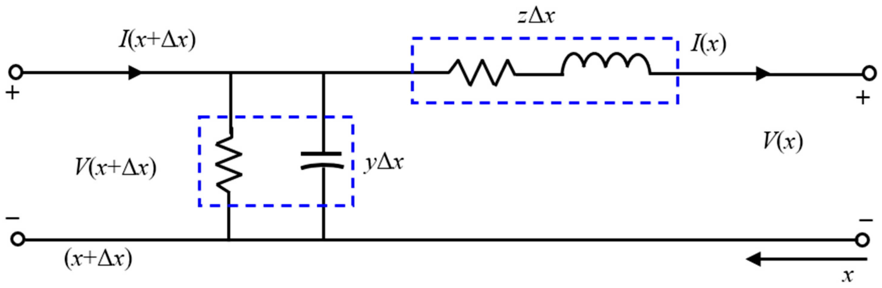
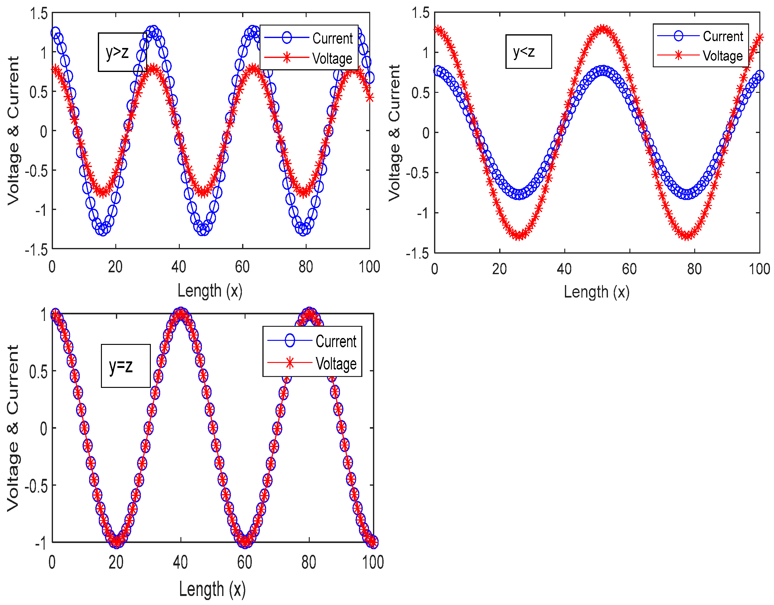
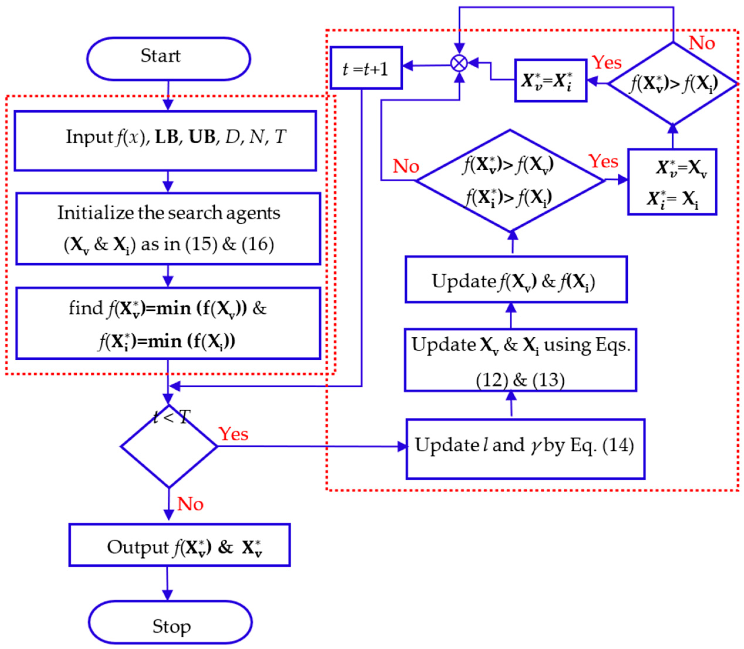
The research gap is defined by the no-free lunch theorem, which states that there is no single algorithm that can succeed in solving all optimization problems. In addition, the mathematical modeling and program coding of some recent metaheuristic algorithms are complex and cannot be easily applied to the online process control of engineering applications. Moreover, some models of algorithms are not investigated by related scientists. Therefore, using a studied mathematical model, simple software code, and fast convergence motivated us to propose a new metaheuristic optimizer called the propagation search algorithm (PSA), stimulated by the propagation of the waveforms of the electrical voltage and current along long transmission lines. Scientists previously offered mathematical voltage and current models at any transmission line section. Then, we adapted these models to be randomized models for random transmission lines with random impedances and admittances. The voltage and current are considered the search agents of the PSA, where they propagate based on their previous values and the propagation constant of the transmission line. These search agents rely on each other’s values, which helps them to encircle the best solution.
The main contributions of this paper are summarized below:
  • Developing a new physics-based metaheuristic algorithm called the propagate search algorithm (PSA), inspired by voltage and current waveform propagation along long transmission lines.
  • Testing the PSA using the 23 famous testing functions and comparing the outcomes with eight famous metaheuristic algorithms.
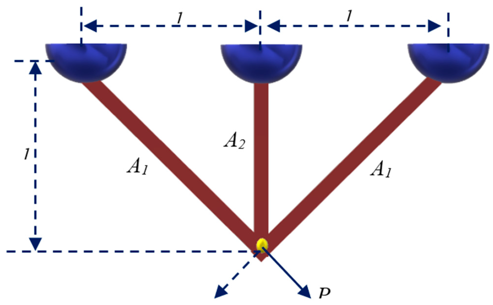
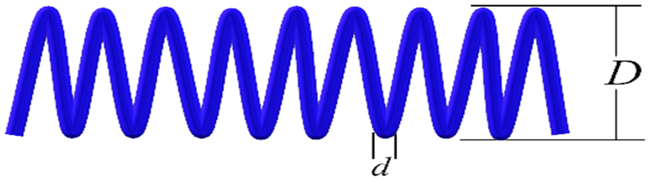
  • Applying the PSA to find the optimum design of four famous engineering problems and comparing it with other metaheuristic algorithms.
The remainder of this paper is designed as follows: Section 2 describes the background, the mathematical modeling, and the flowchart of the proposed PSA; Section 3 describes the testing results; Section 4 shows the application of the proposed PSA to different engineering applications; and Section 5 presents a brief conclusion about the contribution and the results of this paper.

2. Propagation Search Algorithm

The PSA is a physics-based metaheuristic optimization algorithm that is stimulated by the propagation of electrical voltage (V) and current (I) waveforms along long transmission lines, as shown in Figure 1. The parameters of the transmission line, series impedance (z), and shunt admittance (y) play essential roles in the propagation of the voltage and current. For y > z, V(x + Δx) is higher than I(x + Δx); however, for y < z, V(x + Δx) is lower than I(x + Δx), and for y = z, V(x + Δx) is equal to I(x + Δx), as shown in Figure 2. In this work, we will introduce the mathematical modeling of the presented PSA based on the mathematical modeling of the propagation of the voltage and current along the transmission line.

2.1. Background

For a long transmission line, its impedance (z) and admittance (y) are uniformly distributed along its length and cannot be lumped. Therefore, the voltage (V) and current (I) can be calculated at each line section (Δx), as shown in Figure 1. The voltage at any distance can be calculated using Kirchhoff’s voltage law as follows [47]:
V ( x + Δ x ) = ( z Δ x ) I ( x ) + V ( x ) V ( x + Δ x ) V ( x ) Δ x = z I ( x )   lim Δ x 0 V ( x + Δ x ) V ( x ) Δ x = d V ( x ) d x = z I ( x )
For electrical current calculation, Kirchhoff’s current law can be applied as follows:
I ( x + Δ x ) = ( y Δ x ) V ( x + Δ x ) + I ( x ) I ( x + Δ x ) I ( x ) Δ x = y V ( x + Δ x )   lim Δ x 0 I ( x + Δ x ) I ( x ) Δ x = d I ( x ) d x y V ( x )
where V(x + Δx) ≈ V(x), by taking the differential of (1) and substituting it in (2), we can obtain the following:
d 2 V ( x ) d x 2 = z d I ( x ) d x = z y V ( x ) d 2 V ( x ) d x 2 z y V ( x ) = 0
Then, the second-order linear differential equation in (3) can be solved to find V(x), as follows [47]:
V ( x ) = A 1 e z y x + A 2 e z y x
Then, to find the current expression, we will differentiate (4) and compare it with (1), as follows:
d V ( x ) d x = A 1 z y e z y x A 2 z y e z y x = z I ( x )
I ( x ) = z y A 1 e z y x A 2 e z y x z = A 1 e γ x A 2 e γ x Z c
where Zc is the characteristic impedance of the transmission line, Z c = z z y , γ is the propagation constant, γ = z y , and A1 and A2 are constants that can be obtained by solving (6) and (4) for V(0) =VR and I(0) = IR, where VR and IR are the receiving end voltage and current, respectively. Then, we achieve A1 and A2 as follows:
A 1 = V R + Z c I R 2   &   A 2 = V R Z c I R 2
Then, substitute (7) into (4) and (6) to obtain the following:
V ( x ) = V R + Z c I R 2 e γ x + V R Z c I R 2 e γ x = V R e γ x + e γ x 2 + Z c I R e γ x e γ x 2
I ( x ) = V R + Z c I R 2 Z c e γ x V R Z c I R 2 Z c e γ x = V R Z c e γ x e γ x 2 + e γ x + e γ x 2 I R
Then, the hyperbolic functions can be used to represent the exponential expressions as follows:
V ( x ) = V R cosh ( γ x ) + Z c I R sinh ( γ x )
I ( x ) = V R Z c sinh ( γ x ) + I R cosh ( γ x )
For long transmission lines, the series and shunt resistances can be neglected, and only inductance (L) and capacitor (C) are considered. Therefore, z = jωL and y = jωC, so Z c = L / C and γ = j ω L C .

2.2. PSA Inspiration

The PSA is a physics-based metaheuristic optimization algorithm stimulated by the propagation performance of the voltage and current waveforms through a long transmission line. The search agents of the PSA imitate the behavior of the voltage and current. The mathematical model of the PSA is developed based on Equations (10) and (11) with some modifications, as in (12) and (13). The modifications assumed that L = C then Zc = 1 and γ = C, the propagation constant γ is expressed as a random number as in (14), the voltage VR is expressed as Xv, and the current IR is expressed as Xi. The length of the transmission line (l) is the shrinking variable that decreases from 1 to 0, as described in (14).
X v ( t + 1 ) = X v * ( t ) X v ( t ) V R cosh ( γ l ) + ( X i * ( t ) X i ( t ) ) I R sinh ( γ l )
X i ( t + 1 ) = X i * ( t ) X i ( t ) I R cosh ( γ l ) + ( X v * ( t ) X v ( t ) ) V R sinh ( γ l )
l = 1 t / T         t < 0.5 T 1 t / T         t 0.5 T   &   γ = r 1 π r 2         t < 0.5 T r n π 2 r 3         t 0.5 T
where t is the current iteration; T is the total iterations; r1, r2, and r3 are random numbers uniformly distributed between 0 and 1; and rn is a random number generally distributed with a mean of zero. The search agents of the PSA algorithm are Xv and Xi, and the best agents are X v * and X i * .

2.2.1. Search Agents Initialization

The PSA first initializes the vector of the search agent randomly between the lower and upper bounds (LB and UB) with the dimension (1 × D) of a cost function. Initialization plays a vital part in successfully helping the proposed algorithm find the global optimum solution. There are two types of initialization: symmetrical and nonsymmetrical methods. For symmetrical initialization, all elements of the search agent vector are multiplied by the same random number. For the nonsymmetrical initialization, every element is multiplied by a different random number. For the PSA, there are two search agent vectors, Xv and Xi, which can be initialized by any initialization method or by both initialization methods, as in (15).
X v = L B + r × ( U B L B )
X i = L B + R × ( U B L B )
where Xv = [xv1, xv2, xv3, … xvd]T, Xi = [xi1, xi2, xi3, … xid]T, UB = [ub1, ub2, ub3, … ubd]T, LB = [lb1, lb2, lb3, … lbd]T, and R = [r1, r2, r3, … rd]T. The initialization can be conducted for a number n of search agents, so the dimension of all search agents is (N × D).

2.2.2. Exploration and Exploitation of PSA

For better exploration, firstly, the search agents Xv and Xi are initialized differently, as in (15) and (16), which will widen the search areas of the PSA. Secondly, these agents are updated using (12) and (13), where they search in opposite directions for VRIR, as shown in Figure 3. For exploitation of the PSA, the changes of both search agents converge to zero for VR = IR, as shown in Figure 3. Moreover, both search agents are designed to encircle the best solution due to the presence of VR = X v in (12) and IR = X i in (13). The balance between exploration and exploitation is managed by (14), where the first half of total iterations is used for exploitation, and the second half of iterations is utilized for exploration, where the search agents can be diverted using normally distributed random numbers.
For more explanation about exploitation and exploration, two common functions, the Rosenbrock and Rastrigin functions, are used to test the exploration and exploitation of the PSA. Figure 4 shows how the search agents found the best voltage immediately after 10 iterations for the Rastrigin function; however, they were stuck in a local solution for the Rosenbrock function. After t ≥ 0.5 T (at t = 300), the exploration capability of the PSA was activated, and the search agents moved to the best voltage.

2.2.3. Encircling Behavior of PSA

Even though the search agents Xv and Xi of the PSA go in opposite directions, as shown in Figure 3, in the end, they encircle the best solution (X*) because each agent relies on the update step of the other best agent, as shown in (12) and (13). We can notice that the term VR exists in the search agent Xi and the term IR exists in the search agent Xv. Therefore, both search agents encircle the best position, X*. The flowchart of the proposed PSA is depicted in Figure 5.

2.2.4. Computational Complexity of PSA

The complexity of the algorithms varies with the number of loops, the number of search agents (N), and the number of fitness function evaluations. Big O Notation is utilized to measure the computational complexity of PSA. As shown in Figure 4, it starts with the loop of initialization for two kinds of search agents, Xv and Xi, and then the PSA has O(2N) complexity. For the update process and function evaluations, the PSA has O(T × 2N). Therefore, the total complexity of the PSA is O(2N + 2T × N), which can be reduced to the term with the largest order, such as O(2T × N).

3. Optimization Results of Testing Functions

First of all, the robustness of the proposed PSA should be tested using the 23 well-known testing functions. These functions are utilized to verify the exploration and exploitation behaviors of all previously published algorithms. Some of these functions are utilized to test the exploitation ability of the algorithms because they are convex and have one lowest solution, such as the unimodal functions (F1–F7) displayed in Table 1. Other functions are utilized to verify the exploration capability of algorithms to escape being trapped in a local minimum solution because they have different local minimum solutions rather than the global minimum solution, such as the multimodal functions (F8–F23) displayed in Table 2 and Table 3. Then, the minimum values of these functions found by the PSA are compared with those of other renowned algorithms.
In this section, we used eight metaheuristic optimization algorithms besides the PSA. These are the particle swarm optimization (PSO), grey wolf optimizer (GWO), whale optimization algorithm (WOA), sine-cosine algorithm (SCA), transient search optimization (TSO), salp swarm algorithm (SSA), cuckoo search algorithm (CS), and artificial electric field algorithm (AEFA). These algorithms are carefully selected based on the most popular algorithms applied in different engineering applications, such as PSO, GWO, and the WOA. Some of these algorithms are selected because they are inspired by physical behaviors, such as TSO and the AEFA. The remaining algorithms are selected randomly for more comparisons. The values of the algorithms’ parameters are displayed in Table 4.
In this work, the testing experiments are implemented using MATLAB R2023a on Windows 10 64 bits on a Core i7, 16 GB RAM laptop. For an unbiased evaluation, all compared algorithms have a similar number of search agents, N = 30, and the same total number of iterations, T = 500, and all algorithms have the same initialized search agents.

3.1. Statistical Analysis

Due to the random operation of all metaheuristic algorithms, we need to test these algorithms in many independent optimization experiments. Therefore, all optimization algorithms are executed 20 times for each testing function in this paper. Then, the robustness of an algorithm is confirmed by applying different statistical methods, for example, mean (m) and standard deviation (σ) and nonparametric testing methods. Table 5 displays the m and σ of 20 independent runs for all 23 testing functions using the offered PSA and other compared algorithms. The outcomes proved that the offered PSA is competitive with different algorithms and obtained the optimum outcomes for 16 functions out of 23. However, the second competitive algorithm is the CS algorithm, which achieves 9 best functions out of 23 functions.
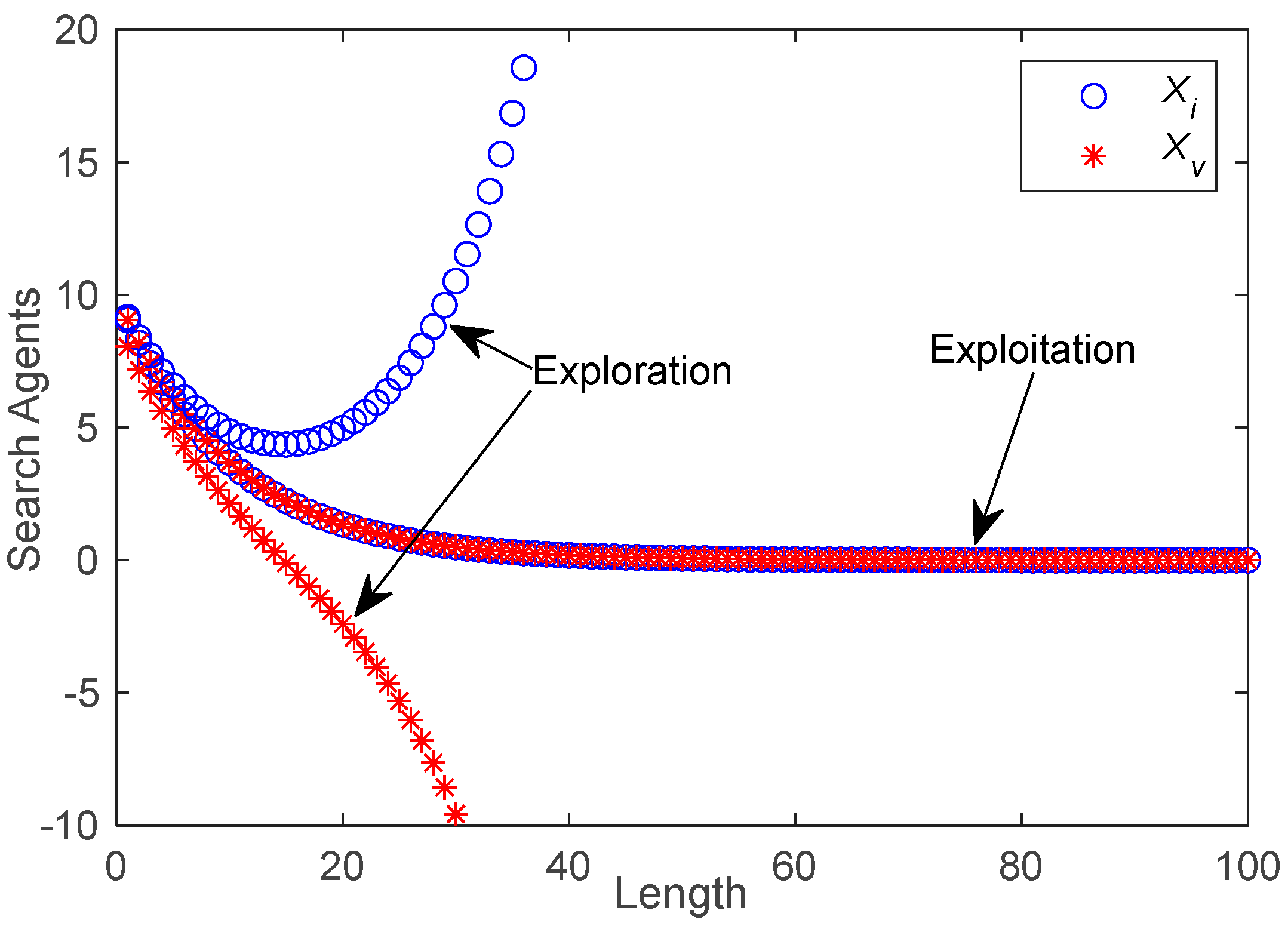
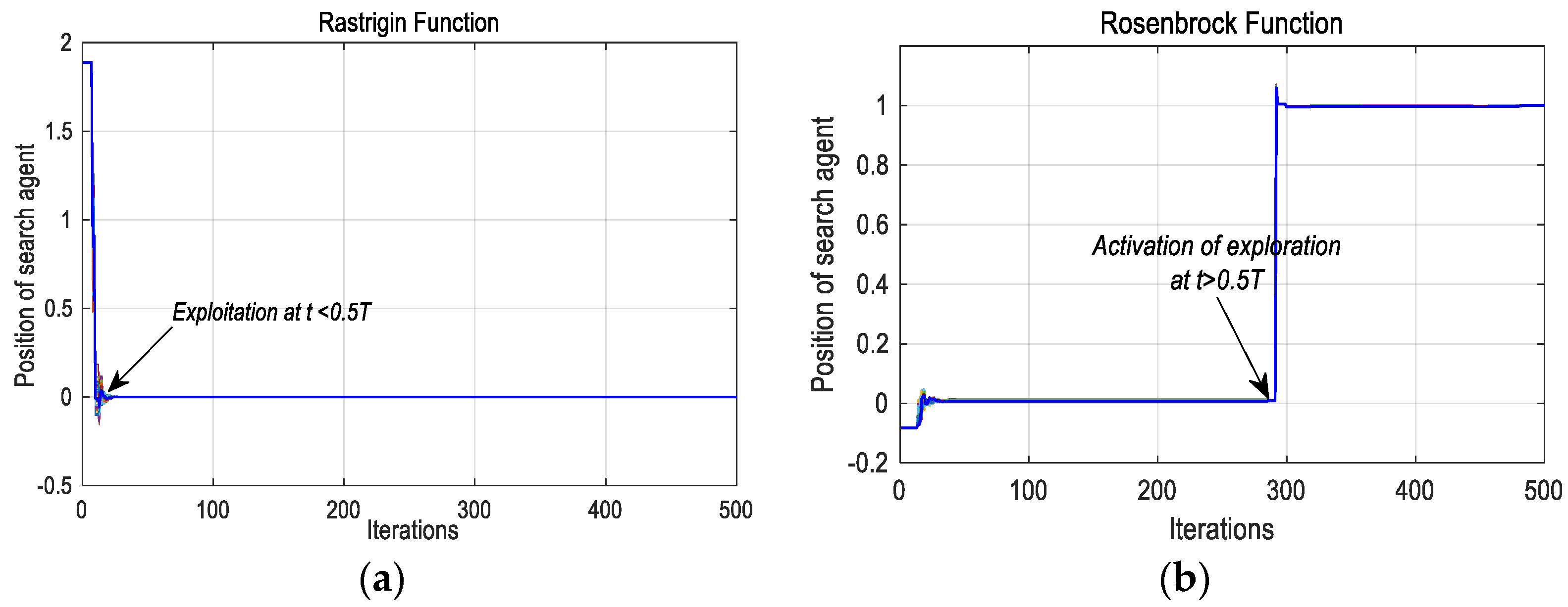
The exploitation of the algorithms is measured using unimodal functions (F1–F8), where the proposed PSA achieved the best outcomes for seven out of eight functions, which proved the exploitation capability of the PSA among other algorithms. On the other side, the exploration capability of the PSA is measured using the multimodal functions (F9–F23). The results show that the PSA obtained the 10 best results out of 15, whereas the CS algorithm achieved second place with the 9 best results out of 15. To check the equilibrium between exploration and exploitation, Rosenbrock (F5) and Rastrigin (F9) are used because they are contrasted, and no algorithm can solve both of them successfully. The results verified that the PSA succeeded in obtaining better results than other algorithms in both types of functions.
Additionally, the Wilcoxon signed-rank test with a 5% significance level is utilized to verify the significance of the PSA among other compared algorithms. This test is a null hypothesis test, which hypothesizes that the results of the PSA and other algorithms are the same if the p-value is higher than 0.05. Table 6 shows the p-values and the denial of the null hypothesis (h = true) or acceptance of it (h = false). We can notice that the most dominant decision is h = true, meaning a significant difference exists between the PSA and other algorithms.
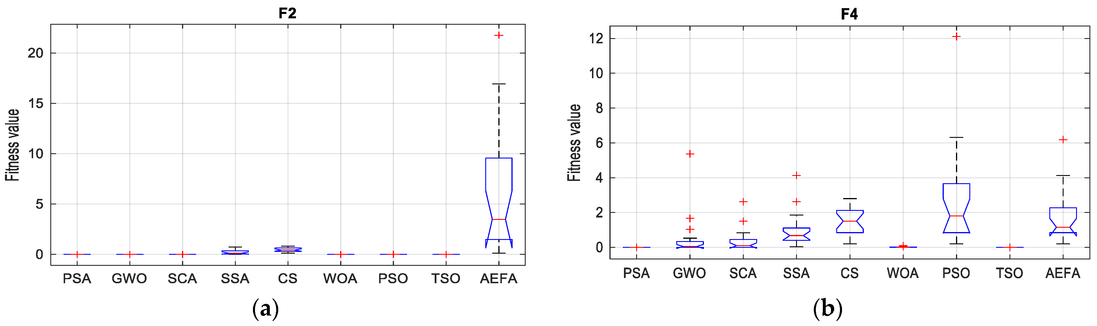
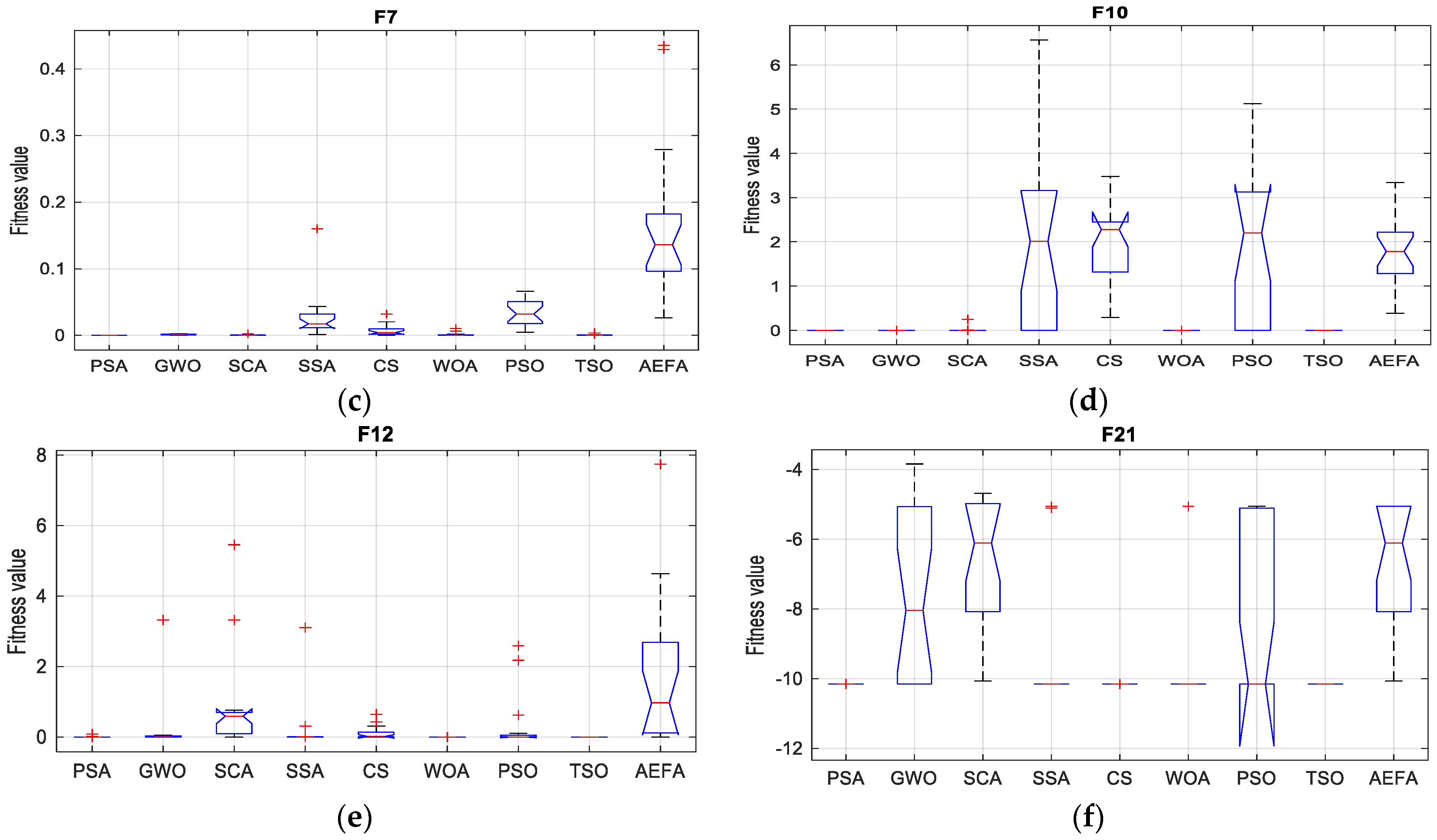
Finally, a boxplot is used for further statistical analysis to verify the performance of the PSA during 20 independent experiments. Figure 6a–f shows the boxplot for six benchmark functions (F2, F4, F8, F10, F12, and F21). The boxplot analysis shows that the PSA has obtained a very small deviation between the maximum and minimum values of 20 experiments. Moreover, it is noticeable that there are outlier points, which are labeled by (+), for all compared algorithm except PSA. Therefore, the boxplot proved the robustness of the PSA over other algorithms.

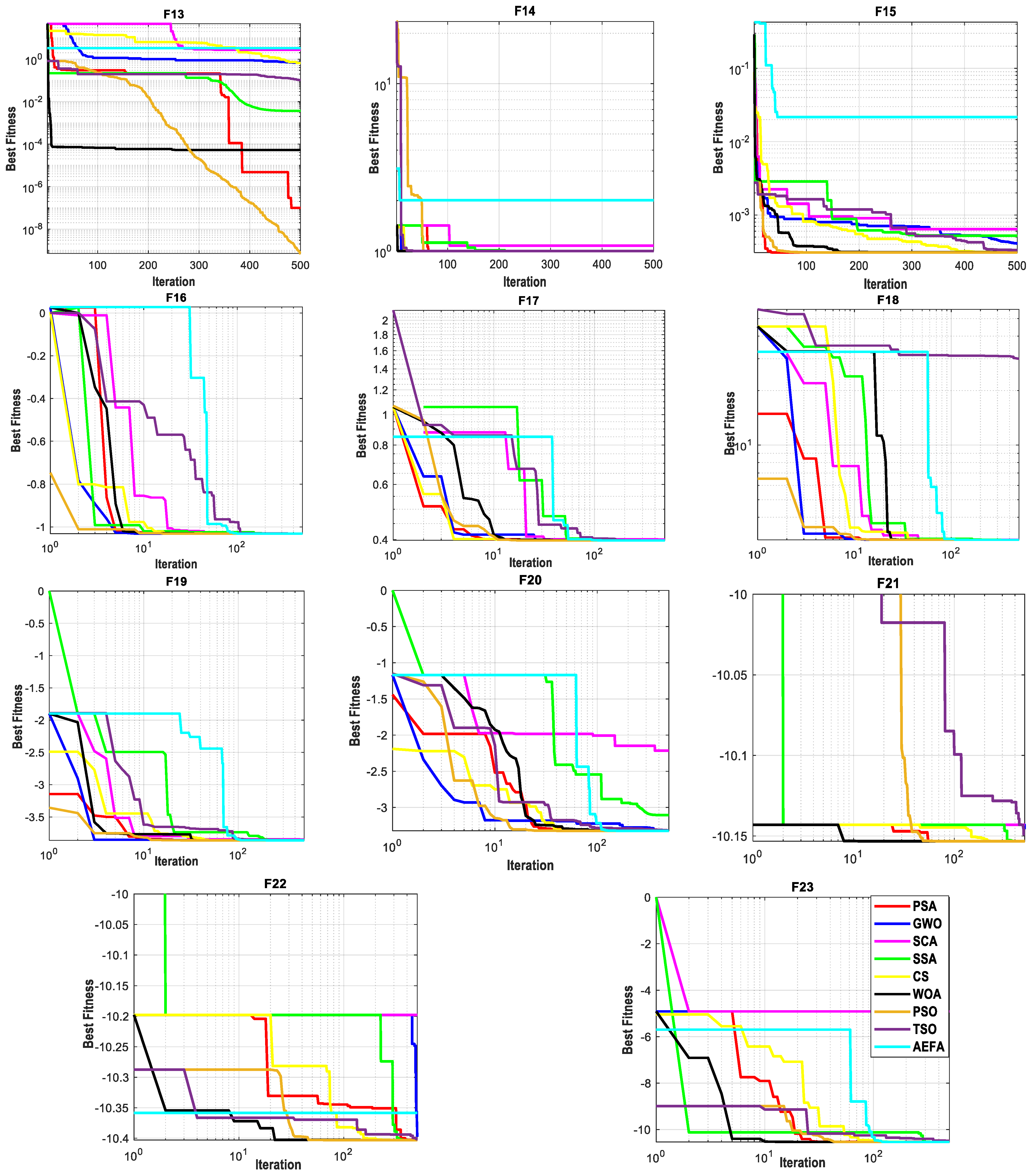
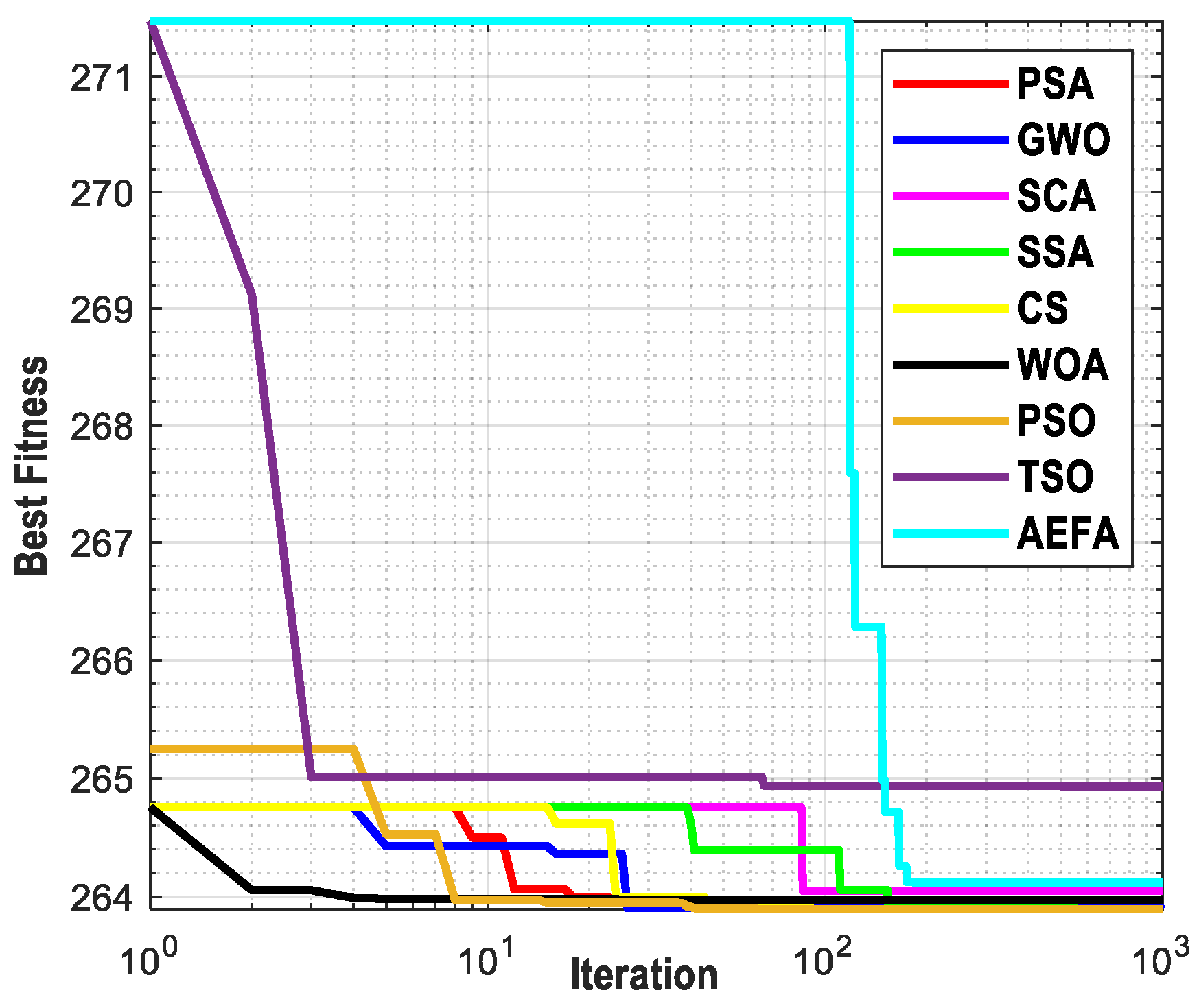
3.2. Optimization Convergence

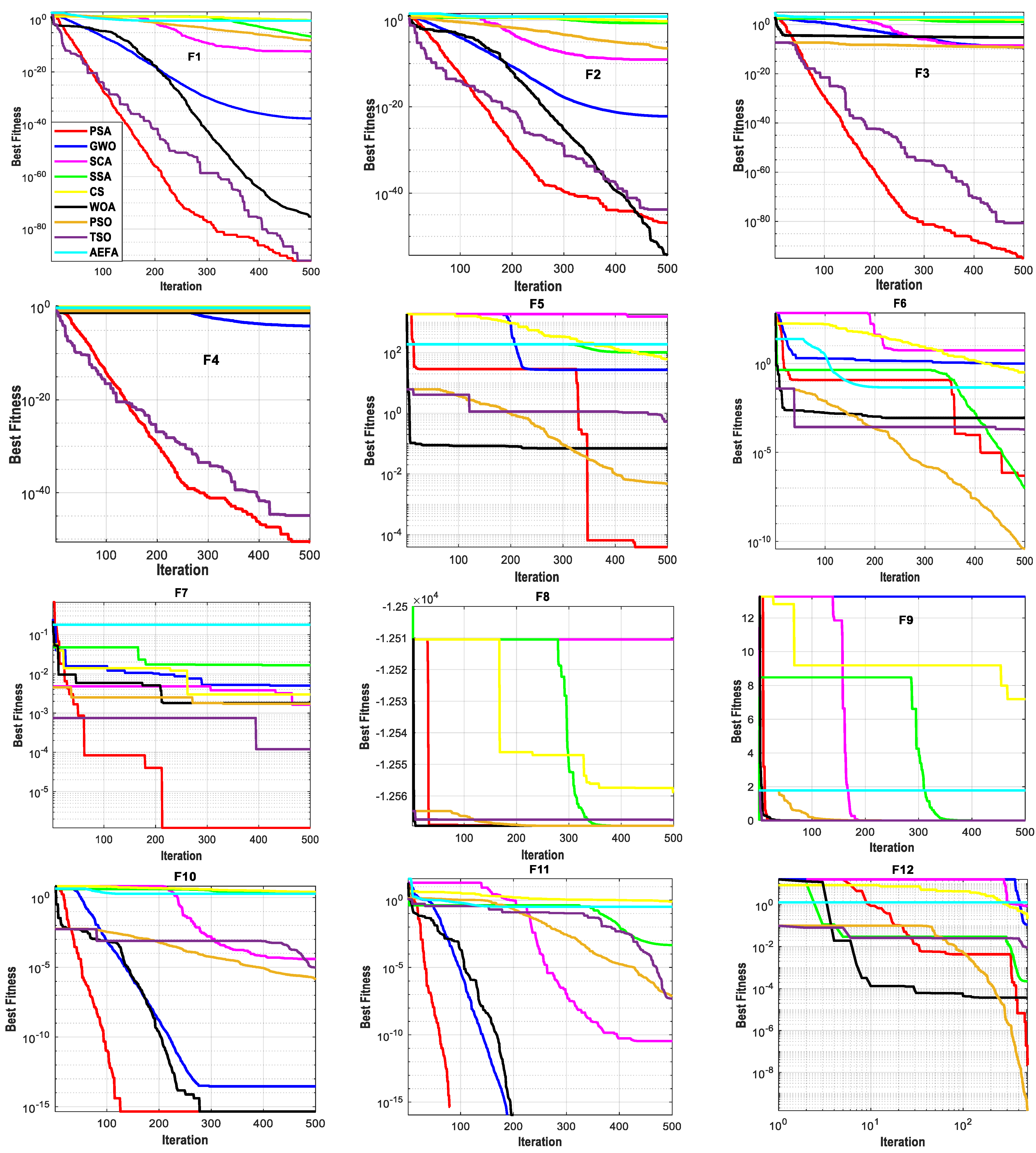
The speed of finding the best solution plays a critical role in control systems, so we need to check the behavior of algorithms with each increment of iterations. Table 7 displays the total elapsed time for all compared algorithms during each independent experiment. However, Figure 7 shows the convergence behavior for all compared algorithms toward the best minimum solution. It is noticeable that all algorithms start from the same initial point for unbiased comparison. The proposed PSA shows fast convergence for the testing functions F1–F8, and then at the middle of total iterations (t = 250) it becomes slower because of changes in the values of the propagation constant (γ). For the remaining functions, the PSA competes with the other algorithms in searching for global solutions; particularly, at t = 250 the PSA escapes being trapped in a local solution.

4. Renowned Engineering Problems

In this section, the offered PSA and other algorithms are utilized to obtain the optimum design of four famous engineering problems, including a three-bar truss structure, a compression spring, a pressure vessel, and a welded beam. The optimization experiments are conducted on MATLAB 2023a on a Windows 10 Core-i7 laptop. The number of search agents is 200, and the total number of iterations is 1000. The mean and standard deviation are calculated for 20 independent code runs.

4.1. Three-Bar Truss Design

Figure 8 depicts the structure of this truss, which is constructed of three bars with different cross-sectional areas (A1, A2, and A3), where A1 = A3. These bars meet at a common node, where a P load is connected to this node. The dimensions between the supporting points of the three bars are equal, which is l, and the vertical dimension between the supporting points and the common node is l too. Reducing the weight of the truss structure is the chief objective, and the design parameters are A1 and A2. The objective function is shown in (17), and the subjected constraints are shown in (18). The PSA is applied to obtain the optimal cross-sectional areas that result in the minimum weight of the three-bar truss. Table 8 displays the outcomes of the optimal areas and the minimum weights obtained using eight algorithms. The statistical results (m and σ) show that the offered PSA has a performance that is comparable with other algorithms, and even better. Moreover, Figure 9 indicates that the PSA converges to the minimum result after only 85 iterations, which is quicker than most of the compared algorithms.
min f ( x = [ A 1 , A 2 ] ) = 2 2 A 1 + A 2 × l
g 1 ( x ) = 2 2 A 1 + A 2 2 A 1 2 + 2 A 1 A 2 P σ 0   &   g 2 ( x ) = A 2 2 A 1 2 + 2 A 1 A 2 P σ 0 g 3 ( x ) = 1 A 1 + 2 A 2 P σ 0   ,   P = 2   kN ,   σ = 2   kN / cm 2 ,   l = 100   cm

4.2. Compression Spring Design

The structure of the compression spring, which is made of steel wire in a spiral form with several coils (N), a material diameter (d), and outer diameter of coil (D), is depicted in Figure 10. Reducing the weight of the compressional spring is the chief objective, where the controlling design parameters are D, d, and N. However, there are constraints to minimizing the weight of the spring, such as the torsional stress, deflection, traveling waves, and dimension. The objective function and the constraint functions of the compression spring design are expressed in (19) and (20). The PSA and other algorithms are applied to find the minimum weight of the compression spring, and the optimal outcomes are presented in Table 9. Furthermore, Figure 11 compares the PSA’s convergence speed with other algorithms, showing that the PSA offers a quicker convergence than most of the compared algorithms, and the PSA converges to the minimum solution after 10 iterations only.
min f ( x = [ D , d , N ] ) = D 2 d ( N + 2 )
g 1 ( x ) = 1 d 3 N 71785 D 4 0   and   g 2 ( x ) = 4 d 2 D d 12566 D 3 ( d D ) + 1 5108 D 2 1 0 g 3 ( x ) = 1 140.45 D N d 2 0   and   g 4 ( x ) = D + d 1.5 1 0 0.05 D 2   &   0.25 d 1.3   &   2.00 N 15

4.3. Welded Beam Design

The structure of the welded beam, which is made by welding a beam to a rigid support member, is depicted in Figure 12. Therefore, reducing the fabrication cost of the welded beam, including labor and material costs, is the main objective, where the controlling design parameters are the dimensions of welding (h) and (l) and the dimensions of the member bar (t) and (b), as shown in Figure 10. However, there are constraints to lessening the cost of the welded beam, such as the weld stress (τ), bending stress (σ), and bar buckling load (Pc). The objective function and the constraint functions of welded beam design are expressed in (21) and (22). The PSA and other algorithms are utilized to find the minimum cost of the welded beam design, and the optimal outcomes are shown in Table 10. Furthermore, Figure 13 compares the PSA algorithm’s convergence speed with other algorithms, showing that the PSA offers a faster convergence speed than most different algorithms, and the PSA converges to the best minimum after only 40 iterations.
min f ( x = [ h   l   t   b ] ) = 1.10471 × h 2 × l + 0.04811 t × b ( 14.0 + l )
g 1 ( x ) = τ τ max 0   and   g 2 ( x ) = σ σ max 0 g 3 ( x ) = δ δ max 0   and   g 4 ( x ) = h b 0 g 5 ( x ) = P P c 0   and   g 6 ( x ) = 0.125 h 0 g 7 ( x ) = 0.10471 × h 2 + 0.04811 × l × b × ( 14.0 + l ) 5.0 0 0.1 h 2   &   0.1 l 10   &   0.1 t 10   &   0.1 b 2
where
P = 6 , 000   l b ; L = 14   i n ; E = 30 × 10 6   p s i ; G = 12 × 10 6   p s i τ max = 13 , 600   p s i ; σ max = 30 , 000   p s i ; δ max = 0.25   i n M = P ( L + l 2 ) ; R = l 2 4 + ( h + t 2 ) 2 ; τ = P 2 h × l ; τ " = M R J
J = 2 2 h × l ( l 2 12 + ( h + t 2 ) 2 ) ; τ = τ 2 + τ τ " l R + τ " 2 P c = 4.013 E L 2 t 2 × b 6 36 ( 1 t 2 L E 4 G ) σ = 6 P L b × t 2 ; δ = 4 P L 3 E × b × t 2

4.4. Pressure Vessel Design

The structure of the pressure vessel, which is made of stainless steel plates that are welded to form a cylindrical shape, is depicted in Figure 14. Therefore, reducing the weight of the pressure vessel is the chief objective, where the controlling design parameters are the dimensions of the vessel, comprising the thickness of the shell (ts), thickness of the head (th), inner radius (r), and length of the vessel (l). However, there are constraints to minimizing the cost of the pressure vessel design, such as the inner volume and the overall size of the vessel. The cost function and the constraint functions of pressure vessel design are expressed in (23) and (24). The PSA and other algorithms are utilized to find the lowest weight of the pressure vessel, and the optimal outcomes are shown in Table 11. Additionally, Figure 15 compares the convergence curve of the PSA with other algorithms, where the PSA offers a quicker convergence than the most of compared algorithms, and the PSA converges to the best minimum after only 50 iterations.
min f ( x = [ T s , T h , R , L ] ) = 0.6224 T s T h L + 1.7781 T h R 2 + 3.1661 T s 2 L + 19.84 T s 2 R
g 1 ( x ) = T s + 0.0193 R 0   &   g 2 ( x ) = T h + 0.00954 R 0 g 3 ( x ) = π R 2 L 4 3 π R 3 + 1 , 296 , 000 0   &   g 4 ( x ) = L 240 0 0 T s 99   &   0 T h 99   &   10 R 200   &   10 L 200

5. Conclusions

In this work, a new physics-based metaheuristic optimization algorithm named the propagation search algorithm (PSA) is offered and utilized to optimize different engineering design problems. First, the exploration and exploitation capabilities of the PSA are confirmed using 23 famous testing functions. The obtained outcomes for the Rosenbrock and Rastrigin functions have confirmed that the PSA has a balanced capability between exploration and exploitation in the optimization procedure. The propagation constant of the PSA controls this balancing capability. The statistical tests are applied to verify the superiority of the PSA among other compared algorithms. The PSA has succeeded in finding the optimal solution for 17 functions out of 23; however, the second-ranked algorithm solved only 9 functions. The Wilcoxon signed-ranked test is applied to confirm the significance level of the outcomes of the PSA compared with those of other algorithms, where 90% of the computed p-values are less than 5%. The PSA and the compared algorithms are utilized to obtain the optimum design of four famous engineering problems, including the three-bar truss, compression spring, welded beam, and pressure vessel. The PSA has succeeded in finding competitive results and fast convergence to the minimum fitness values. The optimization results have shown that the proposed PSA is a promising optimizer that can be easily applied in engineering fields. Finally, the simple form of the PSA limits its performance in some engineering applications. Therefore, the future work will present different enhancements to the PSA and will apply it in power systems.

Author Contributions

Conceptualization, M.H.Q. and H.M.H.; methodology, M.H.Q. and S.A.; software, M.H.Q. and K.H.L.; validation, M.H.Q. and H.M.H.; formal analysis, H.M.H.; investigation, K.H.L. and S.A.; resources, S.A. and H.M.H.; data curation, M.H.Q.; writing—original draft preparation, M.H.Q.; writing—review and editing, H.M.H., K.H.L. and S.A.; visualization, K.H.L. and H.M.H.; supervision, K.H.L., H.M.H. and S.A.; project administration, K.H.L. and M.H.Q. All authors have read and agreed to the published version of the manuscript.

Funding

This research was funded by the Deputyship for Research and Innovation, “Ministry of Education” in Saudi Arabia (IFKSUOR3-328-1).

Data Availability Statement

Not applicable.

Acknowledgments

The authors extend their appreciation to the Deputyship for Research and Innovation, “Ministry of Education”, in Saudi Arabia for funding this research (IFKSUOR3-328-1).

Conflicts of Interest

The authors declare no conflict of interest.

References

  1. Holland, J.H. Genetic Algorithms. Sci. Am. 1992, 267, 66–73. [Google Scholar] [CrossRef]
  2. Kennedy, J.; Eberhart, R. Particle swarm optimization. In Proceedings of the ICNN’95—International Conference on Neural Networks, Perth, Australia, 27 November–1 December 1995; Volume 4, pp. 1942–1948. [Google Scholar]
  3. Dorigo, M.; Di Caro, G. Ant colony optimization: A new meta-heuristic. In Proceedings of the 1999 Congress on Evolutionary Computation-CEC99 (Cat. No. 99TH8406), Washington, DC, USA, 6–9 July 1999; Volume 2, pp. 1470–1477. [Google Scholar]
  4. Karaboga, D.; Basturk, B. On the performance of artificial bee colony (ABC) algorithm. Appl. Soft Comput. 2008, 8, 687–697. [Google Scholar] [CrossRef]
  5. Yang, X.-S. Firefly Algorithms for Multimodal Optimization BT—Stochastic Algorithms: Foundations and Applications; Watanabe, O., Zeugmann, T., Eds.; Springer: Berlin/Heidelberg, Germany, 2009; pp. 169–178. [Google Scholar]
  6. Yang, X.S.; Deb, S. Cuckoo search via Lévy flights. In Proceedings of the 2009 World Congress on Nature and Biologically Inspired Computing, NABIC 2009, Coimbatore, India, 9–11 December 2009; pp. 210–214. [Google Scholar]
  7. Mirjalili, S.; Mirjalili, S.M.; Lewis, A. Grey Wolf Optimizer. Adv. Eng. Softw. 2014, 69, 46–61. [Google Scholar] [CrossRef]
  8. Mirjalili, S.; Lewis, A. The Whale Optimization Algorithm. Adv. Eng. Softw. 2016, 95, 51–67. [Google Scholar] [CrossRef]
  9. Mirjalili, S.; Gandomi, A.H.; Mirjalili, S.Z.; Saremi, S.; Faris, H.; Mirjalili, S.M. Salp Swarm Algorithm: A bio-inspired optimizer for engineering design problems. Adv. Eng. Softw. 2017, 114, 163–191. [Google Scholar] [CrossRef]
  10. Heidari, A.A.; Mirjalili, S.; Faris, H.; Aljarah, I.; Mafarja, M.; Chen, H. Harris hawks optimization: Algorithm and applications. Future Gener. Comput. Syst. 2019, 97, 849–872. [Google Scholar] [CrossRef]
  11. Abdel-Basset, M.; Mohamed, R.; Zidan, M.; Jameel, M.; Abouhawwash, M. Mantis Search Algorithm: A novel bio-inspired algorithm for global optimization and engineering design problems. Comput. Methods Appl. Mech. Eng. 2023, 415, 116200. [Google Scholar] [CrossRef]
  12. Abdel-Basset, M.; Mohamed, R.; Jameel, M.; Abouhawwash, M. Nutcracker optimizer: A novel nature-inspired metaheuristic algorithm for global optimization and engineering design problems. Knowl.-Based Syst. 2023, 262, 110248. [Google Scholar] [CrossRef]
  13. Abualigah, L.; Yousri, D.; Abd Elaziz, M.; Ewees, A.A.; Al-qaness, M.A.A.; Gandomi, A.H. Aquila Optimizer: A novel meta-heuristic optimization algorithm. Comput. Ind. Eng. 2021, 157, 107250. [Google Scholar] [CrossRef]
  14. Hayyolalam, V.; Pourhaji Kazem, A.A. Black Widow Optimization Algorithm: A novel meta-heuristic approach for solving engineering optimization problems. Eng. Appl. Artif. Intell. 2020, 87, 103249. [Google Scholar] [CrossRef]
  15. Kaur, S.; Awasthi, L.K.; Sangal, A.L.; Dhiman, G. Tunicate Swarm Algorithm: A new bio-inspired based metaheuristic paradigm for global optimization. Eng. Appl. Artif. Intell. 2020, 90, 103541. [Google Scholar] [CrossRef]
  16. Kaveh, A.; Farhoudi, N. A new optimization method: Dolphin echolocation. Adv. Eng. Softw. 2013, 59, 53–70. [Google Scholar] [CrossRef]
  17. Braik, M.; Hammouri, A.; Atwan, J.; Al-Betar, M.A.; Awadallah, M.A. White Shark Optimizer: A novel bio-inspired meta-heuristic algorithm for global optimization problems. Knowl.-Based Syst. 2022, 243, 108457. [Google Scholar] [CrossRef]
  18. Abdollahzadeh, B.; Gharehchopogh, F.S.; Mirjalili, S. African vultures optimization algorithm: A new nature-inspired metaheuristic algorithm for global optimization problems. Comput. Ind. Eng. 2021, 158, 107408. [Google Scholar] [CrossRef]
  19. Jiang, Y.; Wu, Q.; Zhu, S.; Zhang, L. Orca predation algorithm: A novel bio-inspired algorithm for global optimization problems. Expert Syst. Appl. 2022, 188, 116026. [Google Scholar] [CrossRef]
  20. Zamani, H.; Nadimi-Shahraki, M.H.; Gandomi, A.H. Starling murmuration optimizer: A novel bio-inspired algorithm for global and engineering optimization. Comput. Methods Appl. Mech. Eng. 2022, 392, 114616. [Google Scholar] [CrossRef]
  21. Wang, L.; Cao, Q.; Zhang, Z.; Mirjalili, S.; Zhao, W. Artificial rabbits optimization: A new bio-inspired meta-heuristic algorithm for solving engineering optimization problems. Eng. Appl. Artif. Intell. 2022, 114, 105082. [Google Scholar] [CrossRef]
  22. Eusuff, M.; Lansey, K.; Pasha, F. Shuffled frog-leaping algorithm: A memetic meta-heuristic for discrete optimization. Eng. Optim. 2006, 38, 129–154. [Google Scholar] [CrossRef]
  23. Qi, X.; Zhu, Y.; Zhang, H. A new meta-heuristic butterfly-inspired algorithm. J. Comput. Sci. 2017, 23, 226–239. [Google Scholar] [CrossRef]
  24. Dhiman, G.; Kumar, V. Spotted hyena optimizer: A novel bio-inspired based metaheuristic technique for engineering applications. Adv. Eng. Softw. 2017, 114, 48–70. [Google Scholar] [CrossRef]
  25. Abualigah, L.; Elaziz, M.A.; Sumari, P.; Geem, Z.W.; Gandomi, A.H. Reptile Search Algorithm (RSA): A nature-inspired meta-heuristic optimizer. Expert Syst. Appl. 2022, 191, 116158. [Google Scholar] [CrossRef]
  26. Dehghani, M.; Montazeri, Z.; Trojovská, E.; Trojovský, P. Coati Optimization Algorithm: A new bio-inspired metaheuristic algorithm for solving optimization problems. Knowl.-Based Syst. 2023, 259, 110011. [Google Scholar] [CrossRef]
  27. Rabie, A.H.; Mansour, N.A.; Saleh, A.I. Leopard seal optimization (LSO): A natural inspired meta-heuristic algorithm. Commun. Nonlinear Sci. Numer. Simul. 2023, 125, 107338. [Google Scholar] [CrossRef]
  28. Mohammadi-Balani, A.; Dehghan Nayeri, M.; Azar, A.; Taghizadeh-Yazdi, M. Golden eagle optimizer: A nature-inspired metaheuristic algorithm. Comput. Ind. Eng. 2021, 152, 107050. [Google Scholar] [CrossRef]
  29. van Laarhoven, P.J.M.; Aarts, E.H.L. Simulated Annealing: Theory and Applications; Springer: Dordrecht, The Netherlands, 1987; pp. 7–15. ISBN 978-94-015-7744-1. [Google Scholar]
  30. Rashedi, E.; Nezamabadi-pour, H.; Saryazdi, S. GSA: A Gravitational Search Algorithm. Inf. Sci. 2009, 179, 2232–2248. [Google Scholar] [CrossRef]
  31. Hashim, F.A.; Houssein, E.H.; Mabrouk, M.S.; Al-Atabany, W.; Mirjalili, S. Henry gas solubility optimization: A novel physics-based algorithm. Future Gener. Comput. Syst. 2019, 101, 646–667. [Google Scholar] [CrossRef]
  32. Kaveh, A.; Dadras, A. A novel meta-heuristic optimization algorithm: Thermal exchange optimization. Adv. Eng. Softw. 2017, 110, 69–84. [Google Scholar] [CrossRef]
  33. Kaveh, A.; Mahdavi, V.R. Colliding bodies optimization: A novel meta-heuristic method. Comput. Struct. 2014, 139, 18–27. [Google Scholar] [CrossRef]
  34. Zhao, W.; Wang, L.; Zhang, Z. Atom search optimization and its application to solve a hydrogeologic parameter estimation problem. Knowl.-Based Syst. 2019, 163, 283–304. [Google Scholar] [CrossRef]
  35. Kaveh, A.; Talatahari, S. A novel heuristic optimization method: Charged system search. Acta Mech. 2010, 213, 267–289. [Google Scholar] [CrossRef]
  36. Kaveh, A.; Khayatazad, M. A new meta-heuristic method: Ray Optimization. Comput. Struct. 2012, 112–113, 283–294. [Google Scholar] [CrossRef]
  37. Qais, M.H.; Hasanien, H.M.; Alghuwainem, S. Transient search optimization: A new meta-heuristic optimization algorithm. Appl. Intell. 2020, 50, 3926–3941. [Google Scholar] [CrossRef]
  38. Abdel-Basset, M.; Mohamed, R.; Azeem, S.A.A.; Jameel, M.; Abouhawwash, M. Kepler optimization algorithm: A new metaheuristic algorithm inspired by Kepler’s laws of planetary motion. Knowl.-Based Syst. 2023, 268, 110454. [Google Scholar] [CrossRef]
  39. Pereira, J.L.J.; Francisco, M.B.; Diniz, C.A.; Antônio Oliver, G.; Cunha, S.S.; Gomes, G.F. Lichtenberg algorithm: A novel hybrid physics-based meta-heuristic for global optimization. Expert Syst. Appl. 2021, 170, 114522. [Google Scholar] [CrossRef]
  40. Abedinpourshotorban, H.; Mariyam Shamsuddin, S.; Beheshti, Z.; Jawawi, D.N.A. Electromagnetic field optimization: A physics-inspired metaheuristic optimization algorithm. Swarm Evol. Comput. 2016, 26, 8–22. [Google Scholar] [CrossRef]
  41. Qais, M.H.; Hasanien, H.M.; Turky, R.A.; Alghuwainem, S.; Tostado-Véliz, M.; Jurado, F. Circle Search Algorithm: A Geometry-Based Metaheuristic Optimization Algorithm. Mathematics 2022, 10, 1626. [Google Scholar] [CrossRef]
  42. Anita; Yadav, A. AEFA: Artificial electric field algorithm for global optimization. Swarm Evol. Comput. 2019, 48, 93–108. [Google Scholar] [CrossRef]
  43. Muthiah-Nakarajan, V.; Noel, M.M. Galactic Swarm Optimization: A new global optimization metaheuristic inspired by galactic motion. Appl. Soft Comput. J. 2016, 38, 771–787. [Google Scholar] [CrossRef]
  44. Formato, R.A. Central force optimization: A new nature inspired computational framework for multidimensional search and optimization. Stud. Comput. Intell. 2008, 129, 221–238. [Google Scholar] [CrossRef]
  45. Javidy, B.; Hatamlou, A.; Mirjalili, S. Ions motion algorithm for solving optimization problems. Appl. Soft Comput. J. 2015, 32, 72–79. [Google Scholar] [CrossRef]
  46. Azizi, M. Atomic orbital search: A novel metaheuristic algorithm. Appl. Math. Model. 2021, 93, 657–683. [Google Scholar] [CrossRef]
  47. Glover, J.D.; Overbye, T.; Sarma, M.S. Power System Analysis and Design, 6th ed.; Cengage Learning: Boston, MA, USA, 2016. [Google Scholar]
Figure 1. Line section of a long transmission line.
Mathematics 11 04224 g001
Figure 2. Effect of z and y on the trajectories of voltage and current.
Mathematics 11 04224 g002
Figure 3. Exploration and exploitation of PSA.
Mathematics 11 04224 g003
Figure 4. Examples of exploitation and exploration of PSA as in (a,b).
Mathematics 11 04224 g004
Figure 5. The flowchart of the PSA.
Mathematics 11 04224 g005
Figure 6. Statistical analysis using boxplot for all compared algorithms.
Mathematics 11 04224 g006aMathematics 11 04224 g006b
Figure 7. The optimization convergence of testing functions using different algorithms.
Mathematics 11 04224 g007aMathematics 11 04224 g007b
Figure 8. Three-bar truss structure.
Mathematics 11 04224 g008
Figure 9. Convergence speed of algorithms to the minimum weight of the three-bar truss design.
Mathematics 11 04224 g009
Figure 10. Compression spring structure.
Mathematics 11 04224 g010
Figure 11. Convergence speed of algorithms to the minimum weight of the compression spring design.
Mathematics 11 04224 g011
Figure 12. Welded beam structure.
Mathematics 11 04224 g012
Figure 13. Convergence speed of algorithms to the minimum cost of the welded beam design.
Mathematics 11 04224 g013
Figure 14. Cylindrical pressure vessel structure.
Mathematics 11 04224 g014
Figure 15. Convergence speed of algorithms to the minimum weight of the pressure vessel design.
Mathematics 11 04224 g015
Table 1. Unimodal testing functions with unfixed dimensions (d).
No.NameFormulaDimension [LB, UB]Minimum
F1Sphere i = 1 d y i 2 d = 30[−100, 100] d0
F2Shwefel
2.22
i = 1 d y i + i = 1 d y i d = 30[−10, 10] d0
F3Shwefel
1.2
i = 1 d ( j = 1 i y j ) 2 d = 30[−100, 100] d0
F4Schwefel
2.21
max i { y i , 1 i d } d = 30[−100, 100] d0
F5Rosenbrock i = 1 d [ 100 ( y i + 1 y i 2 ) 2 + ( y i 1 ) 2 ] d = 30[−30, 30] d0
F6Step i = 1 d ( y i + 0.5 ) 2 d = 30[−100, 100] d0
F7Quartic
Noise
i = 1 d i . y i 4 + r a n d o m [ 0 , 1 ) d = 30[−1.28, 1.28] d0
Table 2. Multimodal testing functions with unfixed dimensions (d).
No.NameFormulaDimension[LB, UB]Minimum
F8Schwefel 2.26 i = 1 d y i sin ( y i ) d = 30[−500, 500] d−418.98 × d
F9Rastrigin i = 1 n [ y i 2 10 cos ( 2 π y i ) + 10 ] d = 30[−5.12, 5.12] d0
F10Ackley 20 exp ( 0.2 1 d j = 1 d y j ) exp ( 1 n cos ( 2 π y j ) ) + 20 + e d = 30[−32, 32] d0
F11Griewank 1 4000 i = 1 d y i 2 i = 1 d cos ( y i i ) + 1 d = 30[−600, 600] d0
F12Penalized π d { 10 sin ( π y 1 ) + i = 1 d ( y i 1 ) 2 [ 1 + 10 sin 2 ( π y i + 1 ) ] + ( y d 1 ) 2 } + i = 1 d u ( x i , 10 , 100 , 4 ) y i = 1 + x i + 1 4   &   u ( x i , a , k , m ) = k ( x i a ) m                   x i > a 0                                                 a < x i < a k ( x i a ) m             x i < a d = 30[−50, 50] d0
F13Generalized Penalized 0.1 × { 10 sin 2 ( 3 π y 1 ) + i = 1 d ( y i 1 ) 2 [ 1 + sin 2 ( 3 π y i + 1 ) ] + ( y d 1 ) 2 [ 1 + sin 2 ( 2 π y d ) ] } + i = 1 d u ( y i , 5 , 100 , 4 ) d = 30[−50, 50] d0
Table 3. Fixed-dimension (d) multimodal testing functions.
No.NameFormulaDimension[LB, UB]Best Solution
F14De Jong Fifth ( 1 500 + i = 1 25 1 i + j = 1 2 ( y i a i j ) 6 ) 1 d = 2[−65, 65] d1
F15 i = 1 11 [ a i y i ( b i 2 + b i y 2 ) b i 2 + b i y 3 + y 4 ] 2 d = 4[−5, 5] d0.00030
F16Six-Hump Camel 4 y 1 2 2.1 y 1 4 + 1 3 y 1 6 + y 1 y 2 4 y 2 2 + 4 y 2 4 d = 2[−5, 5] d−1.0316
F17Branins ( y 2 5.1 4 π 2 y 1 2 + 5 π y 1 6 ) 2 + 10 ( 1 1 8 π ) cos ( y 1 ) + 10 d = 2[−5, 5] d0.398
F18Goldstein–Price [ 1 + ( y 1 + y 2 + 1 ) 2 ( 19 14 y 1 + 3 y 1 2 14 y 2 + 6 y 1 y 2 + 3 y 2 2 ) ] ×                             [ 30 + ( 2 y 1 3 y 2 ) 2 × ( 18 32 y 1 + 12 y 1 2                             + 48 y 2 36 y 1 y 2 + 27 y 2 2 ) ] d = 2[−2, 2] d3
F19Hartmann 3D i = 1 4 c i exp ( j = 1 3 a i j ( y j p i j ) 2 ) d = 3[1, 3] d−3.86
F20Hartmann 6D i = 1 4 c i exp ( j = 1 6 a i j ( y j p i j ) 2 ) d = 6[0, 1] d−3.32
F21Shekel 5 i = 1 5 [ ( Y a i ) ( Y a i ) T + c i ] 1 d = 4[0, 10] d−10.1532
F22Shekel 7 i = 1 7 [ ( Y a i ) ( Y a i ) T + c i ] 1 d = 4[0, 10] d−10.4028
F23Shekel 10 i = 1 10 [ ( Y a i ) ( Y a i ) T + c i ] 1 d = 4[0, 10] d−10.5363
Table 4. The setting of the compared algorithms.
AlgorithmParameters
Proposed PSAl decrease from 1 to 0
PSOweight ω varies between [0.5, 0.3] c1 = c2 = 2
GWOThe variable a changes between [2, 0]
SSAThe probability is 0.5
SCAa = 2 and p = 0.5
CSPa = 0.25, tolerance is 1 × 10⁻⁵, beta = 1.5,
WOAl = 1, a decrease from 2 to 0, a2 decrease from −1 to −2
TSOt decreases from 2 to 0, K = 1, probability update is 0.5
AFEAAlfa = 30, K0 = 500;
Table 5. Mean and standard deviations of 20 independent trials.
No. GWOSCASSACSWOAPSOTSOAEFAPSA
F1m2.954E−384.401E−111.204E−076.780E−011.845E−753.772E−072.037E−771.818E+003.507E−81
σ4.217E−387.184E−117.488E−083.424E−018.119E−755.262E−079.038E−774.526E+001.568E−80
F2m1.798E−224.088E−081.919E−014.904E−014.471E−529.866E−047.933E−409.613E+002.814E−42
σ2.141E−229.436E−081.990E−011.785E−011.355E−513.135E−033.353E−395.891E+008.774E−42
F3m1.465E−081.942E−081.891E+023.220E+022.092E+009.432E+022.050E−728.880E+025.964E−81
σ5.082E−084.062E−083.092E+022.957E+025.104E+001.118E+039.161E−724.508E+022.536E−80
F4m1.022E−018.313E−017.620E−011.083E+001.833E−022.120E+009.245E−401.486E+006.223E−43
σ2.591E−011.103E+006.087E−016.512E−013.710E−022.301E+004.122E−391.199E+001.474E−42
F5m2.161E+015.604E+011.991E+015.693E+017.043E+002.968E+014.282E+016.921E+022.507E−02
σ1.056E+018.190E+011.286E+014.234E+011.228E+012.689E+011.308E+021.143E+034.152E−02
F6m5.181E−015.225E+001.006E−065.647E−016.694E−036.793E−075.687E−011.379E+004.303E−02
σ3.616E−011.234E+003.178E−063.298E−011.232E−021.157E−066.711E−013.051E+001.902E−01
F7m1.701E−035.580E−042.901E−021.043E−027.335E−043.340E−026.114E−032.270E−016.207E−05
σ1.196E−037.296E−042.039E−021.271E−026.587E−042.274E−021.298E−021.791E−016.558E−05
F8m−1.176E+04−1.173E+04−1.239E+04−1.243E+04−1.239E+04−1.234E+04−1.247E+04−1.226E+04−1.257E+04
σ1.174E+031.161E+037.945E+022.125E+027.951E+028.072E+022.035E+024.015E+022.810E−02
F9m5.013E+012.966E+015.970E+001.652E+010.000E+001.323E+014.601E−053.100E+010.000E+00
σ4.214E+014.088E+011.225E+011.156E+010.000E+001.463E+011.111E−041.977E+010.000E+00
F10m1.910E−142.723E−058.452E−011.482E+003.997E−151.493E+009.446E−041.379E+004.441E−16
σ3.972E−157.773E−051.101E+008.255E−012.577E−151.916E+001.101E−031.058E+000.000E+00
F11m1.215E−036.158E−091.418E−026.696E−010.000E+001.746E−028.731E−026.641E−010.000E+00
σ3.741E−031.751E−081.305E−021.297E−010.000E+001.371E−031.968E−024.874E−010.000E+00
F12m4.925E−011.218E+004.070E−028.174E−021.105E−041.371E+001.219E−022.001E+001.433E−05
σ1.417E+001.462E+001.183E−017.730E−022.800E−042.738E+002.050E−021.659E+002.472E−05
F13m3.058E−012.085E+001.750E−013.605E−011.707E−024.397E−034.041E−011.017E+011.076E−02
σ2.599E−018.328E−016.583E−014.287E−015.871E−025.525E−039.038E−011.078E+014.679E−02
F14m1.978E+001.652E+001.048E+009.980E−011.486E+009.980E−019.980E−013.074E+001.147E+00
σ2.643E+009.196E−012.223E−017.675E−162.184E+000.000E+004.434E−082.259E+004.857E−01
F15m1.354E−035.678E−049.093E−043.141E−043.131E−044.319E−043.889E−041.045E−024.438E−04
σ4.475E−033.540E−046.895E−046.6833E−066.186E−061.139E−041.244E−046.900E−032.274E−04
F16m−1.032E+00−1.032E+00−1.032E+00−1.032E+00−1.032E+00−1.032E+00−1.032E+00−1.032E+00−1.032E+00
σ8.071E−089.936E−051.929E−148.823E−178.258E−102.161E−167.439E−062.038E−162.783E−06
F17m3.979E−014.020E−013.979E−013.979E−013.979E−013.979E−013.979E−013.979E−013.979E−01
σ2.293E−064.196E−039.744E−150.000E+001.453E−050.000E+004.011E−050.000E+003.393E−05
F18m3.000E+003.000E+003.000E+003.000E+003.000E+003.000E+003.107E+013.056E+003.000E+00
σ1.935E−056.407E−051.253E−131.585E−158.710E−059.557E−161.209E+002.518E−012.115E−04
F19m−3.860E+00−3.850E+00−3.863E+00−3.863E+00−3.857E+00−3.862E+00−3.731E+00−3.862E+00−3.862E+00
σ3.312E−034.917E−039.363E−112.040E−151.049E−021.762E−033.073E−011.102E−031.400E−03
F20m−3.298E+00−2.696E+00−3.255E+00−3.322E+00−3.294E+00−3.286E+00−3.275E+00−3.322E+00−3.223E+00
σ7.242E−023.335E−011.025E−014.843E−097.383E−026.652E−021.799E−014.556E−168.357E−02
F21m−8.318E+00−7.132E+00−1.015E+01−1.015E+01−9.898E+00−8.373E+00−1.013E+01−7.285E+00−1.015E+01
σ2.229E+002.255E+003.153E−111.500E−081.140E+002.488E+003.212E−022.158E+006.068E−04
F22m−8.548E+00−7.536E+00−9.612E+00−1.040E+01−1.014E+01−8.289E+00−1.038E+01−9.712E+00−1.040E+01
σ2.445E+002.342E+001.932E+001.765E−081.188E+002.656E+005.051E−021.703E+008.270E−04
F23m−8.912E+00−7.562E+00−1.027E+01−1.054E+01−9.995E+00−8.923E+00−1.051E+01−1.054E+01−1.054E+01
σ2.200E+002.216E+001.199E+001.223E−071.664E+002.528E+002.716E−021.578E−152.631E−03
Table 6. Wilcoxon signed-rank test.
No. GWOSCASSACSWOAPSOTSOAEFA
F1p-value6.683E−056.683E−056.683E−056.683E−056.683E−056.683E−056.683E−056.683E−05
htruetruetruetruetruetruetruetrue
F2p-value6.683E−056.683E−056.683E−056.683E−051.03E−046.683E−056.683E−056.683E−05
htruetruetruetruetruetruetruetrue
F3p-value6.683E−056.683E−056.683E−056.683E−056.683E−056.683E−056.683E−056.683E−05
htruetruetruetruetruetruetruetrue
F4p-value6.683E−056.683E−056.683E−056.683E−056.683E−056.683E−056.683E−056.683E−05
htruetruetruetruetruetruetruetrue
F5p-value6.683E−056.683E−056.683E−056.683E−051.32E−031.03E−046.683E−056.683E−05
htruetruetruetruetruetruetruetrue
F6p-value6.81E−046.683E−056.683E−051.20E−043.04E−021.03E−047.80E−042.82E−03
htruetruetruetruetruetruetruetrue
F7p-value6.683E−052.54E−046.683E−056.683E−052.19E−046.683E−051.20E−046.683E−05
htruetruetruetruetruetruetruetrue
F8p-value6.683E−056.683E−051.51E−036.683E−059.11E−017.31E−021.03E−046.683E−05
htruetruetruetruetruetruetruetrue
F9p-value1.32E−044.38E−046.683E−056.683E−05trueE+006.683E−056.683E−056.683E−05
htruetruetruetruefalsetruetruetrue
F10p-value6.81E−056.683E−056.683E−056.683E−056.10E−056.683E−056.683E−056.683E−05
htruetruetruetruetruetruetruetrue
F11p-value5.00E−016.683E−056.683E−056.683E−05trueE+006.683E−056.683E−056.683E−05
hfalsetruetruetruefalsetruetruetrue
F12p-value6.683E−056.683E−052.19E−046.683E−055.75E−016.01E−016.683E−056.683E−05
htruetruetruetruefalsefalsetruetrue
F13p-value2.19E−046.683E−051.32E−036.683E−051.52E−024.78E−013.90E−046.683E−05
htruetruetruetruetruefalsetruetrue
F14p-value4.38E−027.80E−041.16E−036.683E−053.33E−026.683E−055.02E−013.38E−04
htruetruetruetruetruetruefalsetrue
F15p-value1.79E−019.30E−021.11E−022.19E−047.80E−047.94E−015.02E−016.683E−05
hfalsefalsetruetruetruefalsefalsetrue
F16p-value2.54E−046.683E−056.683E−056.683E−051.03E−046.683E−051.87E−026.683E−05
htruetruetruetruetruetruetruetrue
F17p-value3.04E−026.683E−056.683E−056.683E−051.56E−016.683E−052.28E−026.683E−05
htruetruetruetruefalsetruetruetrue
F18p-value1.52E−021.79E−016.683E−056.683E−053.33E−026.683E−056.683E−051.51E−03
htruetruetruetruefalsetruetruetrue
F19p-value3.32E−016.683E−056.683E−056.683E−052.28E−021.32E−032.19E−042.04E−01
hfalsetruetruetruetruetruetruefalse
F20p-value6.42E−036.683E−052.63E−016.683E−052.20E−031.24E−024.55E−036.683E−05
htruetruefalsetruetruetruetruetrue
F21p-value6.683E−056.683E−056.683E−056.683E−058.52E−016.01E−016.683E−051.03E−04
htruetruetruetruefalsefalsetruetrue
F22p-value6.683E−056.683E−057.31E−026.683E−052.63E−013.13E−016.683E−05trueE+00
htruetruefalsetruefalsefalsetruefalse
F23p-value6.683E−056.683E−051.51E−036.683E−054.33E−01trueE+001.63E−046.683E−05
htruetruetruetruefalsefalsetruetrue
Table 7. Elapsed time in seconds for algorithm execution.
GWOSCASSACSWOAPSOTSOAEFAPSA
F10.193960.128070.120760.322970.078440.104890.079010.705720.14529
F30.289080.253330.218230.590930.212270.246970.202470.56620.21162
F50.220240.144190.116690.372830.095570.124280.094450.744230.18258
F70.252700.274620.177850.527650.182400.207200.157720.588860.23347
F90.216670.142380.101900.356080.092750.123640.079370.702940.15709
F110.216080.150830.110070.392850.099110.132380.098830.751620.18998
F130.430910.379460.341720.892110.327390.344800.316210.718610.45095
F150.084820.061250.047540.241000.045620.046030.043420.191390.07792
F170.043810.051140.038050.207850.035010.026290.032710.146070.05805
F190.050450.057390.052810.228910.051900.043910.048800.177140.12969
F210.066740.067950.063470.255040.058450.054840.060270.211410.10314
F230.087500.084960.081940.295820.079100.071600.078260.220820.14134
Sum2.152951.795581.471034.684031.358001.526841.291515.725022.08111
Table 8. Optimal weight and parameters of three-bar truss design.
GWOSCASSACSWOAPSOTSOAEFAPSA
Best263.8959846263.9090923263.9195433263.8958434263.8959030263.8958434263.8969047263.9195433263.8958824
m263.8964313263.9553596264.0115258263.8958434263.9431231263.8958439265.5472387264.0115258263.8984017
σ4.11448E−044.21400E−029.00459E−020.00000E+006.82155E−027.34918E−071.49798E+009.00459E−022.21516E−03
x10.7890053190.7896741310.7884844980.7886751360.7889600130.7886816520.7874769560.7884844980.789351215
x20.4073157990.4055551910.4087878810.4082482860.4074431270.4082298580.4116478660.4087878810.406573046
Table 9. Optimal weight and parameters of compression spring design.
GWOSCASSACSWOAPSOTSOAEFAPSA
Best0.01777570.01273310.01787230.01267210.01279840.01784870.01266680.01965750.0127226
m0.01778730.01280850.02191180.01269770.01364590.01790140.01393090.03368010.0132851
σ0.00000800.00005460.00823400.00001950.00113710.00003730.00157930.01378930.0006535
D0.06899620.05000000.06915420.05151760.05444580.06908120.05196970.05728920.0500000
d0.93350700.31727110.94043140.35252620.42673450.93702520.36350500.50685450.3174241
N2.000000014.05323541.973905511.54392638.11741381.991488910.90195639.816759714.0323211
Table 10. Optimal cost and parameters of welded beam design.
GWOSCASSACSWOAPSOTSOAEFAPSA
Best1.72611666371.77898876722.47198642101.73188323461.73327457371.72485230861.73383776442.47198642101.7250306573
m1.72675810631.82872560873.04076559571.73786528241.79470454801.72485230881.78355025053.04076559571.7327229652
σ5.19265E−042.34891E−023.96367E−014.99296E−033.61117E−025.07366E−104.43964E−023.96367E−015.14617E−03
h0.20572265910.20741986770.15347910960.20601056240.20020290040.20572963980.18240377980.15347910960.2056551204
l3.47184454113.60406169756.85826658313.48378958533.59239406363.47048866564.53585350446.85826658313.4718699729
t9.03828952419.06781667259.55714308749.02949135949.04193707269.03662391048.82762800639.55714308749.0373416776
b0.20583529140.20934024520.23914456160.20652073960.20570314600.20572963980.21558635050.23914456160.2057274905
Table 11. Optimal weight and parameters of pressure vessel design.
GWOSCASSACSWOAPSOTSOAEFAPSA
Best5889.31616366084.96645506288.25809375886.54581066033.97802765942.12670626713.196927226533.63207415886.9897087
m5894.14467576307.24063947009.57193135893.21204526631.86000646101.19992007102.426831396354.38223556077.8295567
σ6.1000446139.9687665874.99741073.8547414493.3610049140.4149521893.372310744235.2712807308.1664002
ts0.77843110.78954090.96528230.77823470.79103260.81006891.08317282.89634020.7783762
th0.38486150.39831700.47714010.38478950.43200660.40041750.51584891.10049710.3846826
r40.328557240.780666950.014588540.321620240.955715441.972480354.059259564.992181840.3199574
l200.0000000200.000000098.2297744200.0000000191.3306399178.203783669.082110151.8458794200.0000000
Disclaimer/Publisher’s Note: The statements, opinions and data contained in all publications are solely those of the individual author(s) and contributor(s) and not of MDPI and/or the editor(s). MDPI and/or the editor(s) disclaim responsibility for any injury to people or property resulting from any ideas, methods, instructions or products referred to in the content.

