Intelligence in Finance and Economics for Predicting High-Frequency Data

Abstract

Forecasting exchange rates is a complex problem that has benefitted from recent advances and research in machine learning. The main goal of this study is to design and implement a method to improve the learning performance of artificial neural networks with large volumes of data using population-based metaheuristics. The micro-genetic training algorithm is thoroughly analyzed using profiling tools to find bottlenecks. We compare the use of a micro-genetic algorithm to predict changes in currency exchange rates on a data set containing more than 500,000 values. To find the best parameters of neural networks, we propose an improved micro-genetic training algorithm by dividing the training data into mini batches. In this case, the improved micro-genetic algorithm proved to be much faster compared to the standard genetic algorithm, while achieving the same prediction accuracy. This allows for the use of this algorithm for just-in-time predictions of high frequency data. Here, neural network models are first created and validated on an existing data set. Then, the new data values can be added to neural network models and retrained in a short time.

1. Introduction

Perhaps the most applied approach to the forecasting of financial time series is the statistical approach [1]. Prognostic tasks in the financial field are solved through econometric and statistical models. Today, the typical models used in the field of time series modeling are the Kalman filter, linear regression or cointegration analysis models. However, since 1983 when O’Donovan [2] showed that they could provide significantly better results, ARIMA models [3,4] have become the most popular models. However, in 1982, Engle [5] showed that the use of ARIMA models in financial modeling is not correct and thus proposed ARCH models for financial modeling that is capable of modeling variable volatility. Nowadays, these are perhaps the most utilized types of statistical models in finance. Banks use these models to determine the risk of their assets through the value at risk (VaR) strategy.

Although the statistical approach is still the dominant technique in the sphere of financial markets today, it does not always achieve satisfactory results. One of the main problems is insufficient prognostic accuracy when forecasting high-frequency, highly dynamic and highly volatile time series. Due to the massive expansion of information technology, other artificial neural network (ANN) models, known as machine-learning models and including classic and soft radial basic function (RBF) models [6,7], have been implemented in financial forecasting. In recent years, ANNs and soft computing have become popular tools for financial forecasters around the world and widely used tools in the domain of financial forecasting. The reason that ANNs have started to be used and are still used for this purpose is that ANNs are universal functional blackbox approximators of a nonlinear type [8,9]. These are very helpful in modeling nonlinear processes that have a priori unknown functional relationships, or where a system of relationships is very difficult to describe mathematically [10]. Moreover, they are also able to model chaotic time series [11].

In addition, many research groups today focus on so-called hybrid models. These are combinations of ANNs and econometric models, combinations of ANNs and ARIMA models, or generalized ARCH (GARCH) and hidden Markov models (HMM). Marcek and Kotillova [12] proposed a classic RBF NN and a soft RBF NN for the forecasting of currencies for daily exchange rate changes for the Czech Koruna (CZK) against the US dollar, and for AUD against the US dollar. To consider predicting electricity demand half an hour ahead from previous half-hourly demands authors using Australian electricity data also proposed an RBF NN trained by genetic algorithm. In [13], another model was proposed to improve the prediction of high-frequency data of USD/CAD using a hybrid RBF NN model with a one-day forecast horizon. Hybridization was performed both by the introduction of a moving average procedure for modeling the error part of the RB activation function and also by teaching the network using a genetic algorithm. Marcek [14] modified the granular RBF NN’s soft architecture, by introducing a feedback error term from the output neuron as an additional synaptic input for the next training cycle. The predictive accuracy of the modified model was compared with ARIMA (1,1,0)/exponential GARCH (1,1) GED; soft granular RBF NN and SVR models on the time series data of daily BUX stocks closing prices for the period January 2004–December 2012. The modified granular RBF NN model significantly outperformed other statistical and intelligent models.

In the study [15], new improved RBF NNs are designed and tested for the decision support of business management. The improvements concern the implementation of new shapes of the activation functions of the generalized normal distribution (GED) type with a search for values of a shape parameter such that these activation functions achieve exciting advantages, such as foul tolerance and forecasting accuracy, over available models. In [16] the authors proposed an artificial neural network foreign exchange rate forecasting (AFERMF) model to predict foreign exchange rates among major currencies, including the US dollar, the Euro (EUR), British pound (GB) and Japanese yen, against the Nigerian naira. The data used were composed of the daily averages and were downloaded from the OANDA website. This model was compared with the best related hidden Markov foreign exchange rate forecasting model (HFERFM). From various tests performed on the results of the train and validation, it was confirmed that the (AFERMF) performs better in estimating foreign exchange rates. In [17] the authors proposed a convolutional deep-learning-based network for foreign exchange rate, crude oil price and gold price predictions. The explanatory variables for this were exchange rate changes among PKR/USD, GBD/USD and HKD/USD currencies. The daily data of exchange rates ranging from early 2008 to late 2018 were utilized. The authors also added sentiment analysis values. Mean absolute error (MAE) and root mean squared error (RMSE) were used as evaluation metrics. The results were obtained through the proposed deep learning methodology with linear and support vector regression models. Their results show that deep learning-based methods perform better than other models.

The last period is characterized by the continuous development of new information technologies and their deployment, not only to a group of users within the academic or scientific community, but also in the commercial sphere, i.e., to broad masses of people in all areas. A further sign of these trends is the increase in the volume of various data over shorter periods, i.e., data with a higher frequency, with which an organization or institution works. Presenting a striking phenomenon wherein economic and financial processes are undertaken with such dynamic behavior. Therefore, in the area of finance many series are now observed monthly, weekly or daily and so series with more than 1000 observations with one-minute resolution are becoming more common.

The previous author’s work [18] proved that ARMA models can be approximated successfully by artificial neural networks trained by genetic and micro-genetic algorithms. Using these nature-inspired algorithms has shown to be faster than the back-propagation learning algorithm, i.e., an analytical training algorithm based on partial derivatives of gradient methods. However, this technique has been shown to be insufficient for large datasets consisting of several hundreds of thousands of values, which can be common in high-frequency trading predictions.

This article discusses the adaptation of nature-inspired techniques for use on large datasets (big data), as the computational complexity of predictive models can grow dramatically for larger datasets. The main objective of this paper is to show that the proposed and analyzed micro-genetic algorithm is much faster than the standard genetic algorithm for training neural networks on large datasets while achieving the same prediction accuracy. In this paper:

• we evaluate and analyze the performance of the machine learning methods proposed in [18] on one-minute prediction of exchange rate changes for the EUR against the Czech koruna currencies (abbreviated EUR/CZK) for a very large data set,
• we adapt statistical feature selection models (ARMA) to perceptron type neural networks trained by genetic and micro-genetic algorithms, and
• we compare the elapsed time spent using a standard genetic learning algorithm with the time spent using a micro-genetic algorithm.

This paper is organized in the following manner. Section 2 introduces the data and the pre-processing of this data used for our research. Section 3 deals with the theoretical background of ARMA family models. The characterization of conventional time series modelling is introduced. The development of statistical forecasting model and its parameter estimation are also discussed. Section 4 discusses the organizational dynamics of networks, capturing the topology of the network and its possible changes during computation. To develop an efficient forecasting system, the methods for implementing learning algorithms, as well as several commercial procedures and software are used and described. Section 5 provides the assessment of prediction results from both learning approaches and verifies their applicability. Concluding remarks are given in Section 6.

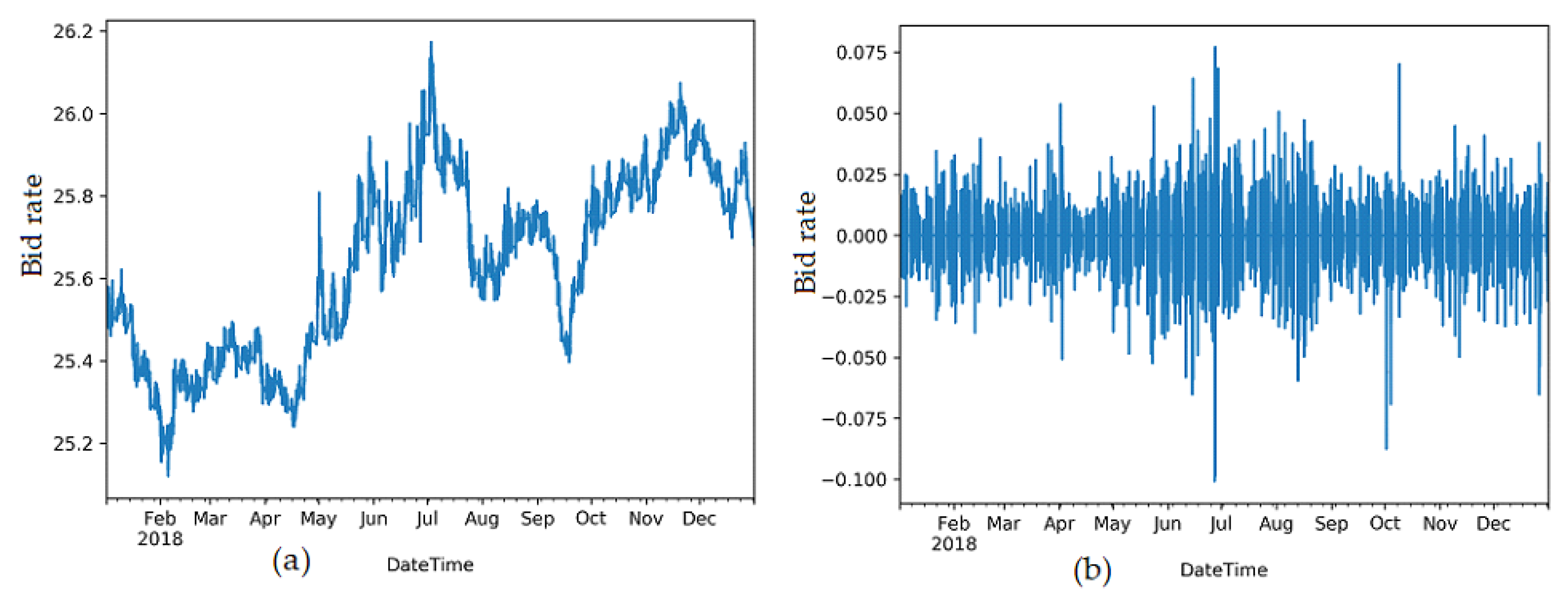
2. Used Data and Its Pre-processing

In this article, as mentioned above, the data set consists of data from high-frequency trading. The data were collected by GAIN Capital company. The data set represents changes in the EUR/CZK exchange rates. The raw data set comprises approximately 521,346 one-minute exchange rate values of bid prices for the year 2018. The time plot of exchange rate price between EUR/CZK without duplicates is available in Figure 1a. In examining Figure 1a, one can see that the series has no zero-mean. Similarly, we also see that this time series exhibits nonstationary behavior in the slope. In order to fit a time series model to the data, we need to first transform the data so that it can be modeled by a zero-mean, stationary ARMA type process. After differentiation, represented by $\{y_t-y_{t-1}\}$ and shown in Figure 1b, the series is stationary in mean and slope. We implemented the algorithm for this data transformation in Python 3.4 (Appendix A). Examining Figure 1b we also note that no significant seasonal variation is observed in the series. At this point, we can conclude that the time series is also non-seasonal.

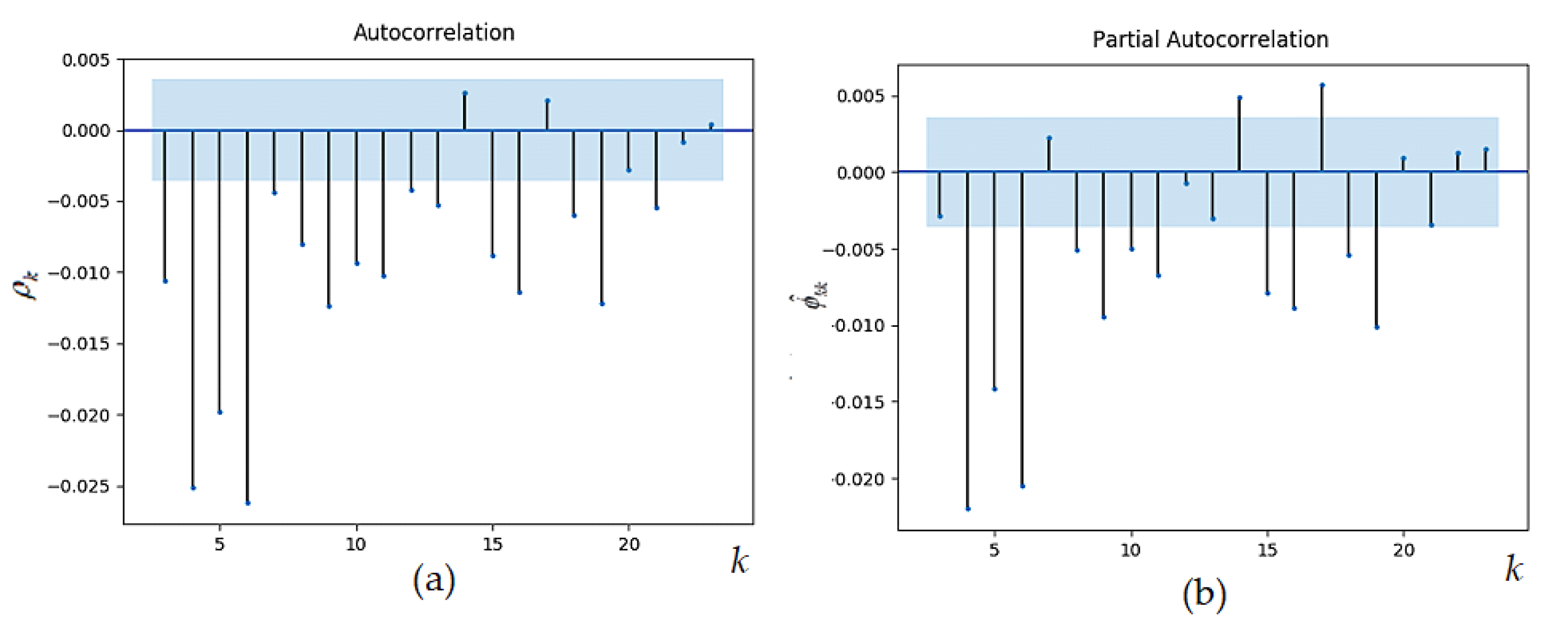
3. Statistical Time Series Analysis and Modelling

As in [18], we assume that, after appropriate transformation, the series is governed by an ARMA model. Identification of the model requires selecting the orders of (p, q), which is the ARMA(p, q) model in the form of

$$y_t={\varphi }_1{y}_{t-1}+{\varphi }_2{y}_{t-2}+\dots +{\varphi }_p{y}_{t-p}-{\theta }_1{\epsilon }_{t-1}-{\theta }_2{\epsilon }_{t-2}-\dots -{\theta }_q{\epsilon }_{t-q}+{\epsilon }_t$$

(1)

where $\{{\varphi }_1,{\varphi }_2,\dots ,{\varphi }_p\}$ and $\{{\theta }_1,{\theta }_2,\dots ,{\theta }_q\}$ represent AR and MA parameters (coefficients) of the autoregressive and moving average parts, respectively, and ${\epsilon }_t$ represents white noise that is normally distributed, i.e., $\epsilon \sim N(0,{\sigma }_{\epsilon }^2)$. Thus, model (1) represents the process containing p autoregressive and q moving average parameters.

The tentative identification of an ARMA time series model is achieved through analysis of actual historical data. The primary tools used in the identification process are the auto correlation function (ACF) and the partial autocorrelation function (PACF). The sample ACF denoted as ${\rho }_k$ can be estimated by the following formula

$${\widehat{\rho }}_k=\frac{\mathrm{cov}(y_{t+k},y_t)}{\sqrt{\mathrm{var}(y_{t+k})\mathrm{var}(y_t)}}$$

(2)

In the estimation of the PACF (denoted as ${\widehat{\varphi }}_{kk}$), different methods of estimating the ARMA parameters are presented, e.g., in the Mathematica software [19]. The estimation of the PACF parameters based on the solving of the Yule–Walker equations is also described in [20]. The standard errors of sample ACF and PACF are useful in identifying mean-zero values. The sample autocorrelation and partial autocorrelation functions for the series are shown in Figure 2a,b, respectively. For assistance in interpreting these functions, two standard-errors limits are plotted on the graphs as blue bands.

We see from Figure 2a,b that the sample autocorrelation function cuts and the sample partial autocorrelation function decays in ways that are approximately sinusoidal, with a relatively large number of nonzero values. Thus, we tentatively identify the underlying model of our series as a stationary ARMA (20, 21) process. Based on the estimated parameters of the ARMA (p, q) model and the calculated test statistics in

Table 1. Estimated parameters for the currency EUR/CZK series data model ARMA (20, 21) and their statistical characteristics. Processed Python 3.4 (Appendix A).

Parameter	Coefficient	Stand. Error	z	p > |z|	[0.025	0.975]
Bias	2.278 × 10−6
ar.L1	−0.9433	0.012	−78.668	0.000	−0.967	−0.920
ar.L2	−0.8507	0.016	−53.408	0.000	−0.882	−0.820
ar.L3	−0.5851	0.017	−33.628	0.000	−0.619	−0.551
ar.L4	−0.7521	0.017	−42.980	0.000	−0.786	−0.718
ar.L5	−0.9723	0.018	−55.435	0.000	−1.007	−0.938
ar.L6	−0.8592	0.020	−42.317	0.000	−0.899	−0.819
ar.L7	−0.8816	0.020	−44.022	0.000	−0.921	−0.842
ar.L8	−0.6486	0.019	−33.298	0.000	−0.687	−0.610
ar.L9	−0.8109	0.018	−44.858	0.000	−0.846	−0.775
ar.L10	−0.8781	0.019	−46.376	0.000	−0.915	−0.841
ar.L11	−0.7273	0.019	−38.855	0.000	−0.764	−0.691
ar.L12	−0.6489	0.018	−35.296	0.000	−0.685	−0.613
ar.L13	−0.8355	0.019	−43.666	0.000	−0.873	−0.798
ar.L14	−0.7791	0.019	−41.321	0.000	−0.816	−0.742
ar.L15	−0.7226	0.019	−38.984	0.000	−0.759	−0.686
ar.L16	−0.6477	0.017	−37.298	0.000	−0.682	−0.614
ar.L17	−0.6149	0.018	−35.131	0.000	−0.649	−0.581
ar.L18	−0.3127	0.015	−20.642	0.000	−0.342	−0.283
ar.L19	0.0190	0.006	2.997	0.003	0.007	0.031
ma.L1	−0.0384	0.012	−3.219	0.001	−0.062	−0.015
ma.L2	−0.0605	0.012	−5.189	0.000	−0.083	−0.038
ma.L3	−0.2482	0.013	−19.002	0.000	−0.274	−0.223
ma.L4	0.1518	0.013	12.111	0.000	0.127	0.176
ma.L5	0.2349	0.013	18.316	0.000	0.210	0.260
ma.L6	−0.0988	0.014	−7.155	0.000	−0.126	−0.072
ma.L7	0.0446	0.014	3.166	0.002	0.017	0.072
ma.L8	−0.2270	0.018	−12.707	0.000	−0.262	−0.192
ma.L9	0.1507	0.019	8.064	0.000	0.114	0.187
ma.L10	0.0842	0.019	4.479	0.000	0.047	0.121
ma.L11	−0.1315	0.019	−6.750	0.000	−0.170	−0.093
ma.L12	−0.0286	0.018	−1.582	0.114	−0.064	0.007
ma.L13	0.1877	0.016	12.059	0.000	0.157	0.218
ma.L14	−0.0507	0.015	−3.428	0.001	−0.080	−0.022
ma.L15	−0.0443	0.013	−3.458	0.001	−0.069	−0.019
ma.L16	−0.0593	0.014	−4.386	0.000	−0.086	−0.033
ma.L17	−0.0065	0.013	−0.492	0.623	−0.033	0.020
ma.L18	−0.2899	0.013	−21.510	0.000	−0.316	−0.264
ma.L19	−0.3137	0.015	−21.118	0.000	−0.343	−0.285
ma.L20	−0.0509	0.020	−2.518	0.012	−0.090	−0.011
ma.L21	−0.0733	0.018	−4.014	0.000	−0.109	−0.038

, we have no evidence to justify rejecting the ARMA (20, 21) model.

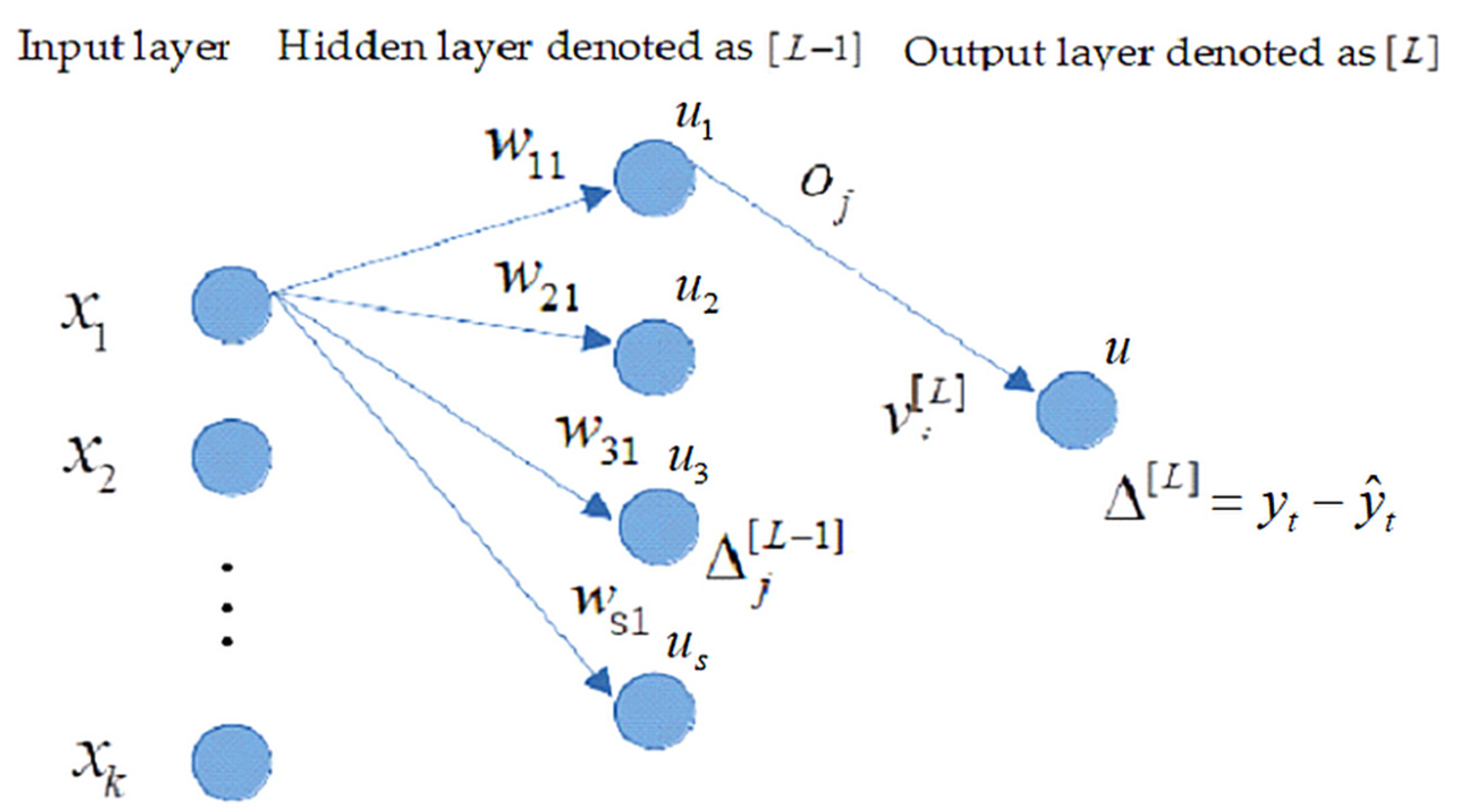
4. The Organizational Dynamics and Implementation of Neural Networks

Organizational dynamics capture the topology of a network, and its possible changes during computation. We utilize organizational dynamics because the topology of a network is proportionate to the complexity of its problems. The most commonly used neural network architecture for the application of time series predictions is the feedforward multi-layered neural network with an error back propagation (BP) learning algorithm, which comprises an input layer, one or more output layers, and one hidden layer of neurons. In Figure 3 the three-layer feedforward network architecture with weights updating in neural network layers is depicted. In this network, the input layer contains “dummy” neurons whose inputs are connected to the outer surroundings and who only distribute input signals to neurons of another layer. The number of input and output neurons is usually given by the character of the task; in our work, the appropriate number of neurons in the hidden layer is based on the minimization of the forecast error function. Additionally, the appropriate number of neurons in the hidden layer is based on the minimization of the forecast error function. It is usual to denote the network topology as numbers of neurons in each layer in the form $(k-s-p)$, where $k$ stands for the input layer, $s$ for hidden layer, and $p$ for output layer. This framework is similar to that used in SVMs. Both techniques are similar in the sense that they consist of a black box principle. ARMA models offer a formal, structured approach to create the architecture of networks. By combining units with multiple intermediate models, ANNs can approximate any smooth non-linearity [21].

As shown in Table 1, the ARMA model is based on 19 auto-regressive (AR) values and one (bias) value, as well as 20 moving average values to predict the currency of the EUR/CZK time series. All p-values are statistically significant at the 5% level of significance. Therefore, the network should have 20 neurons in the input layer. Once an appropriate model has been fit, it may be used to generate forecasts for future observations that are optimal.

Many different forms of mathematical functions can be used to model the nonlinear activation function, such as linear, sigmoidal and radial basis operators. In our network design, the input variables are combined with the $s$ nonlinear intermediate variables, in the second (hidden) layer. Nonlinear intermediate variables are then linearly combined to produce one output variable. The most widely used function in the hidden layer is a sigmoidal function while in the output layer it is a linear function.

4.1. Neural Network Implementation Trained by BP Algorithm

Based on the authors’ experience with the development and applications of commercial software in the area of neural network designs, there are currently several options for using commercial software. One of these is the Deeplearning4j library [22] for the Java platform, for deep learning of feedforward neural networks with vector algebra and arithmetic.

The API of the Deeplearning4j library allows for the easy creation of multi-layered neural networks and allows for the definition of many parameters of layers. However, defining custom activation functions, loss functions or even training algorithms, though technically possible, is rather inconvenient. In the framework of the presented project, the needs of this project were to define a three-layer neural network with bias, hidden layer with sigmoid activation functions, output layer with linear activation and mean squared error (MSE) or loss (error) function. Deeplearning4j already provides optimized implementations of these things, so extending it was not needed in this case. Deeplearning4j also comes with support for splitting both training and evaluation data into minibatches, thus speeding up the process of training. The input data can be in both a vector form defined in ND4j (part of the Deeplearning4j library that focuses on vector and matrix operations) or can be arbitrary, with a user-defined iterator. Since the authors have experience with implementing machine learning algorithms in LISP, which is still popular in machine learning and artificial intelligence, Clojure was chosen as the language for this implementation [23].

Neural network layers $[L]$, $[L-1]$ are described by a collection of matrices or by vectors of weights, vectors of inputs and outputs, and activation functions, in accordance with the following expressions (3)–(5), and by adapting their weights according to expressions (6)–(9) that is (see also Figure 3),

$$a\left((x_1 x_2 \cdots x_k)\times \left(\begin{array}{l}{w}_{11} \dots w_{1s}\\ ⋮\ddots ⋮\\ w_{k1} \dots w_{ks}\end{array}\right)\right)=\left[\begin{array}{l}{o}_1\\ ⋮\\ o_s\end{array}\right]$$

(3)

$$X\times W^{[L-1]}=U^{[L]}$$

(4)

$$a(U^{[L]})=O^{[L]}$$

(5)

where $a$ is an activation function, $X$ is a vector of input data, $W^{[L-1]}$ is a weight matrix for input data vector $X$, $U^{[L]}$ is a column vector of the potentials of hidden layer neurons and $O^{[L]}$ is the column outputs vector from the hidden layer.

• compute the errors for the previous hidden node as

  $${\Delta }_j^{[L-1]}={\Delta }_{}^{[L]} {a^{\prime }}^{[L-1]}(u_j^{[L-1]})v_j^{[L]} \mathrm{for} j=1,\dots ,s$$

  (6)

  where $u_j^{[L-1]}$ is the potential of the previous (hidden) node calculated as

  $$u_j^{[L-1]}=a^{[L-1]}({\displaystyle {\sum }_{r=1}^k{w}_{rj}{}^{[L-1]}{x}_r)} \mathrm{for} j=1,\dots ,s$$

  (7)

  where $a^{[L-1]}$ denotes the activation function at the previous (hidden) [L-1] layer.
• update the weight $v_j$ for the output neuron as

  $${}_{}{}^{new}v_j^{[L]}={}_{}{}^{old}v_j^{[L]}+\eta o_j^{[L-1]}{\Delta }^{[L]} \mathrm{for} j=1,\dots ,s, j=1,\dots ,k$$

  (8)

  where $o_j^{L-1}$ denotes the output from the previous (hidden) layer neurons and $\eta$ represents the learning rate parameter.
• update the weight $w_{rj}^{}$ for the hidden (previous) neurons as

  $${}_{}{}^{new}w_{rj}^{[L-1]}={}_{}{}^{old}w_{rj}^{[L-1]}+\eta {\Delta }_j^{[L-1]}{x}_r \mathrm{for} j=1,\dots ,s; r=1,\dots ,k$$

  (9)

Typically, the updating process is divided into epochs. Each epoch involves updating all the weights for all the examples.

Although we have addressed the training of a classical neural network with a single hidden topology, we have also considered other CNN architectures for deep learning networks with multiple hidden layers and with configurations referenced from the authors [24,25,26]. All these configurations are based on the classical feedforward artificial neural network and therefore adopt most of its basic principles of structure, training and inference. The configurations are built on the basis of the following three principles [27,28,29]: weight sharing, local receptive field and subsampling. The result of sharing is a substantial reduction in the number of free parameters for the maintenance of the number of synapses affecting the network’s ability. The deep learning CNC configuration has three or four types of layers:

• Convolutional layer, whose task is the extraction of various features from the input feature map.

  $$Y_{i,j}^l=b^l+{\displaystyle \sum _{h=1}^H{\displaystyle \sum _{m=1}^K{\displaystyle \sum _{n=1}^K{X}_{i+m,j+n}^h\times W_{m,n}^h}}}$$

  (10)

  where $X_{i+m,j+n}^h$ is a point in the position in $h$ input map, similarly, $Y_{i,j}^l$ is a point at a position $(i,j)$ in the $l$ output map, $W_{m,n}^h$ is the coefficient at the position $(m,n)$ in the $(K\times K\times H)$ dimensional kernel used for the $h$ input map and $b^l$ is the bias for the $l$ output map.
• Pooling layer, which performs the merge operation (11). This operation is essentially the same as in the case of convolutional weaving. The difference lies in the function that is used over a group of points in the local neighborhood. Merging leads to size reduction. In the case of the merging layer, the most used functions are average and maximum. Merging leads to a reduction in the dimensions of maps on other layers, a reduction in the number of synapsis and free parameters.

  $$Y_{i,j}^l=f(X_{i,j}^l,X_{i+1,j}^l,X_{i,j+1}^l,X_{i+1,j+1}^l)$$

  (11)
• Fully-connected layer performs the inner product of the input vector $X$ and the transpose weight vector $W^{\prime }$ plus bias $b_i$, i.e.,

  $$Y_i=X{W}^{\prime }+b_i$$

  (12)

This layer serves as a classifier, where the input vector represents the vector of features extracted in previous layers.

• The rectified linear unit layer is vital in CNN architecture and is based on the non-saturation ‘activation function’. Without activating the fields of the convo layers, it increases the decision function’s nonlinear properties by removing the negative values from the activation map and converting them to zero. For example, rectified linear unit ReLU (13) speeds up network training and calculations.

  $$\mathrm{Re}LU(x)=\max (0,x)$$

  (13)

Due to the operation of CNN in convolutional and fully connected layers, it is obvious that for large volumes of data, as in our task with input data of the order of 10⁴, the solution of using CNN or with classical networks with multiple hidden layers would not lead to the goal. To solve the given types, it is probably more advantageous to use heuristic methods, which are able to find a high-quality approximate solution in a reasonable time. Therefore, we decided to use a network with one hidden layer with the topology in Figure 3 and to train its weights by genetic and micro-genetic algorithms.

4.2. Neural Network Implementation Trained by Genetic Algorithms

A genetic algorithm (GA) simulates the process of evolution, which is controlled Darwin’s principle of natural selection. GA works with a population of individuals—chromosomes. The measure of the quality of an individual is the fitness value. The first population is generated randomly and subsequently evolves from generation to generation by applying selection operators, genetic mutation and the crossing of individuals, while a higher-quality individual has a greater chance of surviving and becoming a parent. These steps are repeated with the aim of improving individuals in the population. Cyclical process of population renewal will end after the fulfillment of predetermined conditions (e.g., after reaching the maximum number of iterations without improvement, etc.). Ideally, the resulting population should contain an individual whose quality is the global optimum of the fitness function.

The basic concept of genetic algorithms, which search for the best admissible (suboptimal) solution to a problem based on Darwinian evolution, as applied in the field of daily exchange rate change prediction using genetically optimized neural networks was first introduced by Nag and Mitra [30].

The weights of the neural network can also be adjusted by GAs. The Clojure 1.6 language was used for both genetic (GA) and micro-genetic (MGA) neural network learning algorithms. In our network, with 20 input neurons and 90 neurons in the hidden layer, the number of genes of an individual was over 4000. Expression (14) shows the way an individual is constructed, where $P$ is a parameter of the network (either weights or bias), $i$ is a gene and $I$ is an individual expressed as a list of genes, i.e.,

$$\{\begin{array}{l}i=\frac{P-P_{\min }}{\left|P_{\max }-P_{\min }\right|}\\ I=(i_1\dots i_n)\end{array}$$

(14)

The selection of individuals for crossing uses the linear rank selection (LRS) technique [18,31,32]. Technically, a linked list is constructed with the worst individual added once, the second worst twice, and so on. Therefore, the best individual in a population of 300 individuals is 300 times more likely to be selected as the worst one. Unlike a technique based solely on the value of loss function, if one individual is much better than others, this does not prevent others from being selected for crossing. Order selection helps prevent the loss of diversity in the population. Predictions are compared to the expected (correct) root mean square error function (loss function) which is calculated for each individual. Since the loss function for an individual does not affect other individuals, its call is parallel.

Technically, the GA does not define the loss function, it only defines a call-back. The loss function is instead left to the calling code and its thread safety.

After sorting the individuals based on their fitness, a rank is assigned to them. The best individual receives rank n, and the worst individual receives rank 1. The selection probability of an individual is given as follows

$$p(i)=\frac{rank(i)}{n(n-1)}$$

(15)

The micro-genetic algorithm is a version of the genetic algorithm that searches for the best admissible (sub-optimal) solution to the problem based on the principle of Darwinian evolution. The micro-genetic algorithms use a very small population size (population size < 20). However, the diversity in the population can be lost. Therefore, the search for the best solution can become stuck in a local minimum. In such a case, it is necessary to save the elites and then to restart the program. The main steps of MGA algorithms, according to Krishnakumar [33] can be as described in Algorithm 1.

Algorithm 1. The main steps of MGA algorithm.

Step 1. Create a random population with 11 individuals (initialization) and go to Step 3. Step 2. Restart: Create a population with 10 individuals randomly and add the one best individual from previous generation. Step 3. Calculate the fitness of individuals. Step 4. Elitism: Determine the best individual from previous generation and keep it for the next generation. Step 5. Selection: Use the rank selection to select 2 pairs of individuals (parents) for crossover. Step 6. Crossover: Determine the cross and add offspring to the new generation. Step 7: Calculate the fitness of individuals. Step 8: Check if there is a loss of diversity. If not go to Step 4 otherwise go to Step 9. Step 9: If termination criterion was not met, go to Step 2, otherwise Stop.

The disadvantage of the standard genetic algorithm is its long calculation time, which is caused by the large number of evaluations of the fitness function of individuals. However, the micro-genetic algorithm works with a small population. Therefore, the calculation time is significantly shorter compared with the standard GA. We can repeat MGA several times when solving a task. By repeating the calculation multiple times, we increase the probability of finding a high-quality solution. The calculation terminates either after performing a certain number of generation or after the set time has elapsed.

The MGAs tend to quickly converge to a state where the population contains only very similar or identical individuals. Progress can then no longer be expected. To check the diversity, we use the convergence parameter $\alpha$, which is defined as follows [34]

$$\alpha =\frac{MS{E}_{\max }-MS{E}_{\min }}{MS{E}_{\min }}$$

(16)

where $MS{E}_{\max }$ is the highest fitness value in a given generation, and $MS{E}_{\min }$ is the smallest fitness value in a given generation. A new population is created by randomly creating new individuals and by adding the best individual from the current population. The implementation of genetic algorithms was modified to work with a smaller population and to allow automatic restarts. A restart is performed when the diversity of the population is lost, i.e., when there are fewer unique individuals than a threshold value predefined by the program.

5. Experiments and Results

Our research focused on testing genetic and micro-genetic algorithms for training neural network weights with the architecture in Figure 3. The experiments were conducted on a set of large, high-frequency time series data obtained and edited from the GAIN Capital company.

In order to increase the efficiency of the calculation, we proceeded to its parallelization using a modified coarse-grained model [35]. The training data were split into minibatches of 1000 samples between individual processes. Each batch then developed relatively independently. When the MSE function for evaluation data started to increase, the training process was stopped because this is a usual sign of overfitting and overtraining of networks.

We verified the forecasting ability of currency changes with two neural network models in the EUR/CZK time series. For our first attempt, we used a standard genetic training algorithm and for our second attempt a micro-genetic training algorithm. Since both networks should approximate a prediction algorithm which predicts one future value, the output layer has one neuron. The linear activation function was chosen for the output neuron. The number of hidden layer neurons ($s$) was found empirically. The best prediction results were achieved when this number was between 90 and 120 neurons. The resulting topology of networks and their possible changes is $(20-s-1)$.

Forty networks were trained for the final performance evaluation, 10 of each of the following four variants: the first trained by genetic algorithm with $s=90$ neurons in the hidden layer, the second trained by genetic algorithm with $s=20$ neurons in the hidden layer, the third trained by micro-genetic algorithm with 90 neurons in the hidden layer and the last trained by micro-genetic algorithm with $s=20$ neurons in the hidden layer.

The configurable parameters regarding GA and MGA are given in

Table 2. Configurable parameters of genetic and micro-genetic algorithms.

Parameter	Standard GA	Micro-GA
Population	1000	10
Elites	5 individuals	1 individual
Crossbreds	220 pairs	3 pairs
Mutants	1% chance either elite or crossbred	2% chance either elite or crossbred
Randoms	1000 − (elites + crossbreds + mutants)	10 − (elites + crossbreds + mutants)
Restart	–	Diversity under 75%

. The computer used for these computations had a four-core AMD A8-6600K processor, 12 GB of RAM, an SSD and used the Linux-based operating system Ubuntu 20.4.

Table 3. The empirical assessment of the two presented GA algorithms.

Parameter	Standard GA 90 Neurons	Standard GA 120 Neurons
Elapsed time [min]	4.104 × 103	4.350 × 103
MSE on validation data set	4.51 × 10−6	4.47 × 10−6
Number of generations	3.741 × 103	3.550 × 103
	Micro-GA	Micro-GA
Elapsed time [min]	4.70 × 102	1.686 × 103
MSE on validation data set	4.41 × 10−6	4.39 × 10−6
Number of generations	49.567 × 103	295.641 × 103
Number of restarts	2.027 × 103	6.965 × 103

presents the average results above the achieved values of the following parameters: elapsed time, MSE on the validation data set (the statistical summary measure of a network’s forecast accuracy), number of generations and number of restarts. We see that the network with the micro-genetic training algorithm achieved better results. In terms of prediction accuracy, all simulations performed with high accuracy, but the best result was obtained when training a network with a micro-genetic algorithm with 120 hidden neurons.

Our work solves the problem of training a neural network’s parameters with population-based metaheuristics. We will present the results of the achieved forecast accuracy results in [17], where the authors present the foreign exchange rate prediction results for the Hong Kong Dollar against the US Dollar (HKD/USD). The achieved prediction accuracy obtained through the proposed deep learning convolutional neural network was much worse, at MSE = 0.017. Otherwise, it is very difficult to compare the work with other works, because it is difficult to find good sources that deal with forecasts with files of big data.

The results of the tests in percentage values are shown in

Table 4. The empirical assessment of the two presented GA algorithms. Values are expressed in percentages (see text for details).

Parameter	Standard GA 90 Neurons	Standard GA 120 Neurons	Micro-GA 90 Neurons	Micro GA 120 Neurons
Elapsed time	94%	100%	1%	1%
MSE on validation data set	100%	99%	98%	97%
Number of generations	1%	1%	16%	100%
Number of restarts	not applicable	not applicable	29%	100%

. The first column lists the names of the parameters used in the training of the networks. The next two columns show the training algorithm types. The first three rows show the achieved values of elapsed time, MSE, and number of generations for the standard GA training algorithms with 90 and 120 neurons in the middle layer of the network. The next three lines show the parameter values as in the first three lines for the training algorithms. In all parameters (except the MSE parameter), the highest achieved value of the parameter was chosen as the basis of 100% when calculating the percentage share. For the MSE parameter, when calculating the percentage share, the lowest achieved value of the parameter was chosen as the basis of 100%.

From Table 3 and Table 4, regarding the comparison of the prediction accuracy of the MSE-based models, it can be seen that the MGA models are more accurate. When comparing the elapsed time to obtain these predictions, the lowest times were achieved by the GA models, which was due to the significantly fewer generations performed by the GA models compared with the MGA models.

6. Conclusions

In this paper, we presented artificial neural networks with an alternative technique for the optimization of their parameters. This was undertaken because the standard learning technique is considered a weakness in standard or radial basic function (RBF) neural networks. As part of our research, we have arrived at a solution for the training of neural networks using genetic algorithms that allow the prediction of high-frequency time series with large volumes of data. For this purpose, we have used and experimentally verified coarse-grained GA models, which benefit from the advantages of GAs and parallel computing.

The computer used for these computations had a four-core AMD A8-6600K processor, 12GB of RAM, an SSD and was running a Linux-based operating system (Ubuntu 20.4).

References

1. Gooijer, J.G. De Gooijer and Rob J. Hyndman. 25 years of time series forecasting. Int. J. Forecast. 2006, 22, 443–473. [Google Scholar] [CrossRef] [Green Version]
2. O’Donovan, T.M. Short Term Forecasting: An Introduction to the Box-Jenkins Approach; Wiley: New York, NY, USA, 1983; ISBN1 10: 0471900133. ISBN2 13: 9780471900139. Available online: https://www.amazon.com/Short-Term-Forecasting-Introduction-Box-Jenkins/dp/0471900133 (accessed on 1 January 1983).
3. Box, G.E.P.; Jenkins, G.M. Time Series Analysis: Forecasting and Control; Holden Day: San Francisco, CA, USA, 1976. [Google Scholar]
4. Ngo, T.H.D.; Bros, W. The Box-Jenkins Methodology for Time Series Models. In SAS Global Forum 2013; Statistics and Data Analysis; Entertainment Group: Burbank, CA, USA, 2013; pp. 201–454. [Google Scholar]
5. Engle, R.F. Autoregressive Conditional Heteroscedasticity with Estimates of the Variance of United Kingdom Inflation. Econom. Econom. Soc. 1982, 50, 987–1007. [Google Scholar] [CrossRef]
6. Gupta, M.M.; Rao, D.H. On the Principles of Fuzzy Neural Networks. Fuzzy Sets Syst. 1994, 61, 1–18. [Google Scholar] [CrossRef]
7. Kecman, V. Learning and soft computing: Support vector machines, neural networks, and fuzzy logic. In Fitting Neural Networks, Scaling of the Inputs, Number of Hidden Units and Layers; The MIT Press: Cambridge, MA, USA, 2001; pp. 353–358. ISBN 9780262527903. [Google Scholar]
8. Hornik, K. Some new results on neural network approximation. Neural Netw. 1993, 6, 1069–1072. [Google Scholar] [CrossRef]
9. Maciel, L.S.; Ballini, R. Design a Neural Network for Time Series Financial Forecasting: Accuracy and Robustness Analysis. 2008. Available online: https://www.cse.unr.edu/~harryt/CS773C/Project/895-1697-1-PB.pdf (accessed on 1 March 2008).
10. Darbellay, G.A.; Slama, M. Forecasting the short-term demand for electricity: Do neural networks stand a better chance? Int. J. Forecast. 2000, 16, 71–83. [Google Scholar] [CrossRef]
11. Zhang, G.; Patuvo, B.E.; HU, M.Y. Forecasting with Artificial Neural Networks: The State of the Art. Int. J. Forecast. 1998, 14, 35–62. [Google Scholar] [CrossRef]
12. Marcek, D.; Kotillova, A. Statistical and Soft Computing Methods Applied to High Frequency Data. J. Mult.-Valued Log. Soft Comput. 2016, 6, 593–608. [Google Scholar]
13. Falat, L.; Marcek, D.; Durisova, M. Intelligent Soft Computing on Forex: Exchange Rates Forecasting with Hybrid Radial Basis Neural Network. Sci. World J. 2016, 2016, 15. [Google Scholar] [CrossRef] [Green Version]
14. Marcek, D. Forecasting of Financial Data: A Novel Fuzzy Logic Neural Network Based on Error Correction Concept and Statistics. Complex Intell. Syst. 2018, 4, 95–104. [Google Scholar] [CrossRef] [Green Version]
15. Marcek, D.; Babel, J.; Falat, L. Forecasting Currency Pairs with RBF Neural Network Using Activation Function Based on Generalized Normal Distribution Experimental Results. J.Mult.-Valued Log. Soft Comput. 2019, 33, 539–563. [Google Scholar]
16. Philip, A.A.; Taofiki, A.A.; Bidemi, A.A. Artificial Neural Network Model for Forecasting Foreign Exchange Rate. Intell. Learn. Syst. Appl. 2011, 3, 57–69. [Google Scholar] [CrossRef] [Green Version]
17. Yasir, M.; Mehr, Y.D.; Sitara Afzal, S.; Mazzan, M.; Farhan, A.; Irfan, M.; Seungmin, R. An Intelligent Event-Sentiment-Based Daily Foreign Exchange Rate Forecasting Systém. Appl. Sci. 2019, 9, 2980. [Google Scholar] [CrossRef]
18. Marcek, D. Some statistical and CI models to predict chaotic high-frequency financial data. J. Intell. Fuzzy Syst. 2020, 39, 6419–6439. [Google Scholar] [CrossRef]
19. Time Series Pack–Reference and Users’s Guide–Wolfram Research. In The Mathematica Applications Library; Wolfram Research, Inc.: Champaign, IL, USA, 1995; pp. 86–99.
20. Montgomery, D.C.; Lynwood, A.J.; Gardiner, J.S. Forecasting and time series analysis. In Autoregressive Integrated Moving Average Models; McGraw-Hill, Inc.: New York, NY, USA, 1900. [Google Scholar] [CrossRef]
21. Crespo, Á.G.; Palacios, R.C.; Gómez-Berbis, J.M.; Mencke, M. BMR: Benchmarking Metrics Recommender for Personnel issues in Software Development Projects. Int. J. Comput. Intell. Syst. 2009, 2, 250–256. [Google Scholar]
22. Available online: https://deeplearrning4j.org (accessed on 18 September 2015).
23. Available online: https://clojure.org/ (accessed on 18 September 2015).
24. Nielsen, M.A. Neural Networks and Deep Learning. Determination. Press 2015. Available online: http://neuralnetworksanddeeplearning.com/www.deeplearningbook.org (accessed on 22 September 2017).
25. Wang, K.; Li, K.; Zhou, L.; Hu, Y.; Cheng, Z.; Liu, J. Multiple convolutional neural networks for multivariate time series prediction. Neurocomputing 2019, 360, 107–119. [Google Scholar] [CrossRef]
26. Liu, S.; Ji, H.; Wang, M.C. Non-pooling Convolutional Neural Network Forecasting for Seasonal Time Series With Trends. IEEE Trans. Neural Netw. Learn. 2020, 31, 2879–2888. [Google Scholar] [CrossRef] [PubMed]
27. Sze, V.; Chen, Y.H.; Yang, T.T.; Emer, J.S. Efficient processing of deep neural networks: A tutorial and Survay. Proc. IEEE 2017, 105, 2295–2329. [Google Scholar] [CrossRef] [Green Version]
28. Hrabovský, J. Detection of Network Attacks in High-Speed Computer Networks. Ph.D. Thesis, University of Žilina, Faculty of Management Science and Informatics, Žilina, Slovakia, 2019. no.: 28360020193008 (In Slovak). [Google Scholar]
29. LeCun, Y.; Bengio, Y. Convolutional networks for images, speech, and time series. English (US). In The Handbook of Brain Theory and Neural Networks; MIT Press: Cambridge, MA, USA, 1995. [Google Scholar]
30. Nag, A.K.; Mitra, A. Forecasting Daily Foreign Exchange Rates Using Genetically Optimized Neural Networks. J. Forecast. 2002, 21, 501–512. [Google Scholar] [CrossRef]
31. Saini, N. Review of Selection Methods in Genetic Algorithms. Int. J. Eng. Comput. Sci. 2017, 6, 22261–22263. [Google Scholar] [CrossRef]
32. Jebari, K.; Madiafi, M.; Elmoujaid, A. Parent Selection Operators for Genetic Algorithms. Int. J. Eng. Technol. 2013, 2, 1141–1145. [Google Scholar]
33. Krishnakumar, K. Micro-genetic Algorithms for Stationary and Non-stationary Function Optimization. In Proceedings of the SPIE Intelligent Control and Adaptive Systems, Philadelphia, PA, USA, 1–3 November 1989; pp. 289–296. [Google Scholar] [CrossRef]
34. Alajmi, A.; Wright, J. Selecting the most efficient genetic algorithm sets in solving unconstrained building. optimization problem. Int. J. Sustain. Built Environ. 2014, 1, 18–26. [Google Scholar] [CrossRef]
35. Crainic, T. Parallel solution methods for vehicle routing problems. In The Vehicle Routing Problem: Latest Advantages and New Challenges; Golden, B., Raghavan, S., Wasil, E., Eds.; Springer: New York, NY, USA, 2008; pp. 171–198. [Google Scholar]
Figure 1. The time plot of exchange rate price between EUR/CZK from January 2018 17:01:00 to 31 December 2018 16:58:00 without duplicates (a), and after first differencing (b). Processed in Python 3.4 (Appendix A).
Mathematics 11 00454 g001
Figure 2. Sample autocorrelation (a) and partial autocorrelation function (b) for the first difference of exchange rate changes for the currency EUR/CZK. Processed in Python 3.4 (Appendix A).
Mathematics 11 00454 g002
Figure 3. Weights updating in neural network layers (see Equations (6)–(9)).
Mathematics 11 00454 g003