Article

Modeling Income Data via New Parametric Quantile Regressions: Formulation, Computational Statistics, and Application

1
Department of Statistics, University of Brasilia, Brasilia 70910-900, Brazil
2
Department of Statistics, Federal University of Rio Grande do Norte, Natal 59078-900, Brazil
3
School of Industrial Engineering, Pontificia Universidad Católica de Valparaíso, Valparaíso 2362807, Chile
4
Faculty of Sciences, Universidad Católica del Maule, Talca 3480112, Chile
5
ANID-Millennium Science Initiative Program-Millennium Nucleus Center for the Discovery of Structures in Complex Data, Santiago 7820244, Chile
*
Author to whom correspondence should be addressed.
Mathematics 2023, 11(2), 448; https://doi.org/10.3390/math11020448
Submission received: 20 December 2022 / Revised: 7 January 2023 / Accepted: 10 January 2023 / Published: 14 January 2023

Abstract

:
Income modeling is crucial in determining workers’ earnings and is an important research topic in labor economics. Traditional regressions based on normal distributions are statistical models widely applied. However, income data have an asymmetric behavior and are best modeled by non-normal distributions. The objective of this work is to propose parametric quantile regressions based on two asymmetric income distributions: Dagum and Singh–Maddala. The proposed quantile regression models are based on reparameterizations of the original distributions by inserting a quantile parameter. We present the reparameterizations, properties of the distributions, and the quantile regression models with their inferential aspects. We proceed with Monte Carlo simulation studies, considering the performance evaluation of the maximum likelihood estimation and an analysis of the empirical distribution of two types of residuals. The Monte Carlo results show that both models meet the expected outcomes. We apply the proposed quantile regression models to a household income data set provided by the National Institute of Statistics of Chile. We show that both proposed models have good performance in model fitting. Thus, we conclude that the obtained results favor the Singh–Maddala and Dagum quantile regression models for positive asymmetrically distributed data related to incomes. The economic implications of our investigation are discussed in the final section. Hence, our proposal can be a valuable addition to the tool-kit of applied statisticians and econometricians.

1. Introduction

Income modeling is essential in determining workers’ earnings and is an important research topic in labor economics. Income data are often modeled using mean-based regressions based on normality, but income is unequally distributed. Thus, this type of data usually has an asymmetric behavior, and then the mean is not an appropriate centrality measure. Hence, quantile regression is generally more helpful in this context [1,2,3]. Quantile regression is a robust alternative to traditional mean-based models and is being widely applied [4,5]. This is because instead of using the mean, these models are based on quantiles, such as median [6]. The quantile approach provides flexibility in modeling, as it allows us to consider the effects of covariates throughout the whole spectrum of the response. Thus, quantile regression also permits us to include the impact on the median, which is a measure of central tendency better than the mean in an asymmetric framework.
Income modeling begins in [7], stating a law on how the income distribution works. Then, this law suggested the well-known Pareto distribution. Such a distribution has set a reference for other models, such as the log-normal and gamma distributions, to show their potential when describing incomes [8,9]. Even though the Pareto, log-normal, and gamma models 10,11] are the most used distributions to describe income data, because of their abilities to describe this type of data, they have limitations. On the one hand, the Pareto model is appropriate to describe only the upper tail of the distribution. On the other hand, the log-normal and gamma distributions perform poorly in describing both the upper and lower tails of the income distributions. Other income distributions, such as the Dagum and Singh–Maddala models, have outperformed the Pareto, log-normal, and gamma distributions when fitting real income data [12,13].
The Dagum distribution was proposed in [14,15] and is widely flexible [16]. This distribution has strictly decreasing and unimodal probability density functions (PDFs), and allows us to fit different types of income data well. The distribution obeys the weak Pareto law, that is, it asymptotically approaches the Pareto distribution. The Dagum model accommodates heavy tails well and it has other characteristics commonly found in income data that are not shared by well-known distributions—such as the log-normal and Pareto models [13,17,18]. The Singh–Maddala distribution was derived from the concept of hazard rate, an approach widely used in the reliability literature [19]. The Singh–Maddala model also obeys the weak Pareto law, and one of its advantages is that it is more flexible than other income distributions. The Dagum and Singh–Maddala distributions are special cases of the generalized beta distribution of the second kind; for more details on these models, one may refer to the works presented in [17,20,21,22].
Several parametric quantile regression models have been proposed in the literature considering diverse distributions [3,23,24,25,26,27,28,29,30,31,32,33,34,35]. The reader is referred to [36] for a full overview of parametric quantile regressions, their applications and computational implementations, which are helpful to model indexes, proportions, and rates. However, to the best of our knowledge, parametric quantile regressions based on the Dagum and Singh–Maddala distributions have not been considered until now. Therefore, the objective of this work is to derive novel parametric quantile regressions based on the Dagum and Singh–Maddala distributions. We first introduce reparameterizations of these two distributions by inserting quantile parameters and then developing the new regression models. We demonstrate that the proposed models outperform the recently proposed Birnbaum–Saunders quantile regression [37,38] in terms of model fitting.
The rest of this article proceeds as follows. In Section 2, we describe the Dagum and Singh–Maddala distributions and propose reparameterizations of these distributions in terms of a quantile parameter. In this section, we also state some properties of such distributions, including their modes and moments. In Section 3, we introduce the quantile regression models, estimate their parameters using the maximum likelihood (ML) method, and present residuals as a diagnostic tool. In this section, we also carry out a Monte Carlo simulation study to evaluate the performance of the ML estimators and of the generalized Cox–Snell (GCS) and randomized quantile (RQ) residuals. Section 4 applies the Dagum and Singh–Maddala quantile regressions to income data from Chile. In Section 5, we present some economic statements, conclusions, and future work.

2. Traditional and Quantile-Based Income Distributions

In this section, we describe the standard Singh–Maddala and Dagum distributions along with the proposed quantile-based reparameterizations of these distributions, which will subsequently be helpful for developing the parametric quantile regression models. We also present properties for each model, including their modal values and moments.

2.1. Singh–Maddala Distribution

If a random variable Y has a Singh–Maddala distribution with shape ( a , q > 0 ) and scale ( b > 0 ) parameters, then we use the notation Y SM ( a , b , q ) .
The Singh–Maddala PDF and cumulative distribution function (CDF) are given by
f SM ( y ; a , b , q ) = a q ( y / b ) a 1 b [ 1 + ( y / b ) a ] 1 + q , F SM ( y ; a , b , q ) = 1 1 + ( y / b ) a q , y > 0 ,
respectively. The Singh–Maddala distribution includes as special cases the Lomax distribution when a = 1 , and the log-logistic distribution when q = 1 . If Y follows a Singh–Maddala distribution, then 1 / Y follows a Dagum distribution, and vice versa. The τ -th quantile of Y SM ( a , b , q ) is obtained by inverting the CDF given in (1), which yields
q ( τ ; a , b , q ) = b c q 1 / a , c q = ( 1 τ ) 1 / q 1 , 0 < τ < 1 .

2.2. Quantile-Based Singh–Maddala Distribution

From the quantile function stated in (2), we find that the most parsimonious way of conducting the reparameterization is using the scale parameter b. Thus, we can write
b = γ c q 1 / a ,
where γ = q ( τ ; a , b , q ) > 0 . Then, the quantile-based Singh–Maddala (QSM) PDF is given by
f QSM ( y ; a , γ , q ) = a q c q ( y / γ ) a 1 γ [ 1 + c q ( y / γ ) a ] 1 + q , y > 0 ,
and we employ the notation Y QSM ( a , γ , q ) .
If Y QSM ( a , γ , q ) , then the following properties hold:
  • (QSM1) Mode [20,39]:
    a 1 a q + 1 1 / a , a > 1 .
  • (QSM2) Moments [20,39]:
    E ( Y r ) = q γ r c q r / a B ( 1 + r / a , q r / a ) , a < r < a q ,
    where B denotes the beta function.
  • (QSM3) Truncated moments [20]:
    E ( Y r 1 { Y > x } ) = a q γ r ( γ / x ) a q r ( a q r ) c q q 2 F 1 1 + q , q r a ; q r a + 1 ; ( γ / x ) a c q , a q > r ,
    where 2 F 1 denotes the Gauss hypergeometric function and 1 is the indicator function.

2.3. Dagum Distribution

The PDF and CDF of a random variable Y following a Dagum distribution with shape ( a , p > 0 ) and scale ( b > 0 ) parameters, denoted by Y DA ( a , b , p ) , are given by
f DA ( y ; a , b , p ) = a p ( y / b ) a p 1 b [ 1 + ( y / b ) a ] 1 + p , F DA ( y ; a , b , p ) = 1 + ( y / b ) a p , y > 0 ,
respectively.
Notice that f DA ( y ; a , b , p ) = ( y / b ) a ( p 1 ) f SM ( y ; a , b , p ) and that when p = 1 both PDFs coincide with the log-logistic distribution. The τ -th quantile of Y DA ( a , b , p ) is stated as
q ( τ ; a , b , p ) = b e p 1 / a , e p = τ 1 / p 1 , 0 < τ < 1 .

2.4. Quantile-Based Dagum Distribution

By observing the three parameters of the traditional Dagum distribution, isolating the scale parameter according to the quantile produces the simplest form of the new quantile-based Dagum distribution. For γ = q ( τ ; a , b , p ) > 0 , this form is represented as
b = γ e p 1 / a .
Hence, we employ the notation Y QDA ( a , γ , p ) and PDF of Y can be written as
f QDA ( y ; a , γ , p ) = a p ( y / γ ) a p 1 γ e p p [ 1 + e p 1 ( y / γ ) a ] 1 + p , y > 0 .
If Y QDA ( a , γ , p ) , then the following properties hold:
  • (QDA1) Mode [39]:
    γ e p 1 / a a p 1 p + 1 1 / p , a p > 1 .
  • (QDA2) Moments [39]:
    E ( Y r ) = γ r e p r / a B a + r p , 1 r p , a p < r < p .
  • (QDA3) Truncated moments:
    E ( Y r 1 { Y > x } ) = p γ r ( γ / x ) a ( 1 a r ) ( 1 a r ) e p p 2 F 1 1 + p , 1 a r ; 2 a r ; ( γ / x ) a e p 1 , a r < 1 .
Proof (Proof of Property (QDA3)).
If Y QDA ( a , γ , p ) , then
E ( Y r 1 { Y > x } ) = x y r a p ( y / γ ) a p 1 γ e p p [ 1 + e p 1 ( y / γ ) a ] 1 + p d y .
Taking the change of variables z = e p 1 ( y / γ ) a and d z = a e p 1 ( y / γ ) a 1 d y / γ , we obtain
E ( Y r 1 { Y > x } ) = p γ r e p a r + p 1 e p 1 ( x / γ ) a z a r + p 1 ( 1 + z ) 1 + p d z .
Consider u x a 1 ( 1 + b x ) ν d x = u a ν b ν ( ν a ) 1 2 F 1 ( ν , ν a ; ν a + 1 ; 1 / ( b u ) ) , for ν > a ; see Eq. (3.194.2) in [40]. Then, we have that
E ( Y r 1 { Y > x } ) = p γ r ( γ / x ) a ( 1 a r ) ( 1 a r ) e p p 2 F 1 1 + p , 1 a r ; 2 a r ; ( γ / x ) a e p 1 , a r < 1 ,
and the proof follows.    □

2.5. Summary Table and PDF Plots

Table 1 presents the Singh–Maddala and Dagum distributions in their original and quantile-based versions.
Figure 1 displays PDF shapes of the quantile-based income distributions for different combinations of parameters, considering scenarios where a, p, q, and γ are fixed. In the Singh–Maddala model, we can see that a influences the kurtosis and skewness, while q changes the kurtosis, as it decreases when q increases. In the Dagum model, we see a similar pattern for a, changing both kurtosis and skewness, while p affects the kurtosis.

3. Income Quantile Regression Models

In this section, we formulate income quantile regressions models as well as the estimation of their parameters and model diagnostics. Moreover, we present Monte Carlo simulation studies for each reparameterized quantile model, considering different parameters and sample size scenarios.

3.1. Formulation

Let Y 1 , , Y n be independent random variables such that each Y i , for i { 1 , , n } , has PDF given by some reparameterized income distribution defined in Table 1, for a fixed (known) level τ ( 0 , 1 ) associated with the quantile of interest. Then, in the formulation of the Singh–Maddala and Dagum quantile regression models, the parameter γ of Y i assumes the functional relation stated as
g ( γ i ) = x i β ( τ ) ,
where β ( τ ) = ( β 0 ( τ ) , , β k ( τ ) ) is the vector of the unknown regression coefficients, which are assumed to be functionally independent, with β ( τ ) R ( k + 1 ) and k + 1 < n . In addition, we have that x i = ( x i 1 , , x i l ) are the values of l covariates, for i { 1 , , n } . Furthermore, we assume that the design matrix X = ( x 1 , , x n ) has rank l. The link function g : R + R defined in (3) must be strictly monotone, positive, and at least twice differentiable, with g 1 being the inverse function of g. Here, we work with the logarithm function as the link structure since it is widely used and more flexible in our simulation studies.

3.2. Estimation

Consider a sample of size n, Y 1 , , Y n say, such that Y i QSM ( a , γ i , q ) , with i { 1 , , n } . Then, the corresponding likelihood function for θ = ( β ( τ ) , a , q ) is expressed as
L ( θ ) = i = 1 n a q c q ( y / γ i ) a 1 γ i [ 1 + c q ( y / γ i ) a ] 1 + q ,
where γ i is given in (3). By applying logarithm in (4), we obtain the log-likelihood function as
( θ ) = i = 1 n ( a 1 ) log ( a q c q ( y / γ i ) ) log ( γ i ) + ( 1 + q ) log ( 1 + c q ( y / γ i ) a ) .
Now, consider a sample of size n, Y 1 , , Y n say, such that Y i QDA ( a , γ i , p ) , with i { 1 , , n } . Then, the corresponding likelihood function for θ = ( β ( τ ) , a , p ) is established as
L ( θ ) = i = 1 n a p ( y / γ i ) a p 1 γ i e p p [ 1 + e p 1 ( y / γ i ) a ] 1 + p .
By applying logarithm in (6), we obtain the log-likelihood function as
( θ ) = i = 1 n ( a p 1 ) log ( a p ( y / γ i ) ) p log ( e p γ i ) + ( 1 + p ) log ( 1 + e p 1 ( y / γ i ) a ) .
To obtain the ML estimate of θ , it is necessary to maximize the log-likelihood functions defined in (5) and (7). Therefore, we need to differentiate the log-likelihood functions to find the score vector ˙ ( θ ) and then equate it to zero, providing the likelihood equations. They are solved using the Broyden–Fletcher–Goldfarb–Shanno (BFGS) quasi-Newton method [41]. This method is implemented in the R software. Under some regularity conditions [42] and when n is large, the asymptotic distribution of the ML estimator θ ^ = ( β ^ ( τ ) , a ^ , q ^ ) (QSM) or θ ^ = ( β ^ ( τ ) , a ^ , p ^ ) (QDA) is asymptotically multivariate normal, that is, θ ^ ˙ N k + 3 ( θ , Σ 1 ( θ ) ) , where ˙ means `approximately distributed’ and Σ ( θ ) is the expected Fisher information matrix, which is given by Σ ( θ ) = E [ θ / θ θ ] . A consistent estimator of Σ ( θ ) is the estimated observed Fisher information matrix, given by K ( θ ^ ) = θ / θ θ | θ = θ ^ . Then, we can approximate Σ ( θ ) by K ( θ ^ ) .

3.3. Diagnostics

Departures from regression model assumptions and goodness of fit are often assessed utilizing residual analysis. Particularly, we use the GCS and RQ residuals defined as r ^ i GCS = log ( 1 F Y ( y i ; θ ^ ) ) and r ^ i RQ = Φ 1 ( F Y ( y i ; θ ^ ) ) , for i { 1 , , n } , where F Y is quantile-based Singh–Maddala or Dagum CDF, and θ ^ is the ML estimate of θ . If the model is correctly specified, the GCS residual is asymptotically standard exponential distributed, while the RQ residual is asymptotically standard normal distributed. With both residuals, graphical techniques, such as quantile–quantile (QQ) plots with simulated envelope, can be used to assess the adequacy of the distribution assumption.

3.4. Simulations

Next, we present Monte Carlo simulations for each reparameterized quantile model, considering different parameters and sample size scenarios. The first part of the study evaluates the performance of the ML estimation of the model parameters, while the second one assesses the empirical distribution of the GCS and RQ residuals. Both studies consider simulated data generated from the Singh–Maddala and Dagum quantile regression models according to γ i = exp β 0 ( τ ) + β 1 ( τ ) x 1 i + β 2 ( τ ) x 2 i , for i { 1 , , n } .
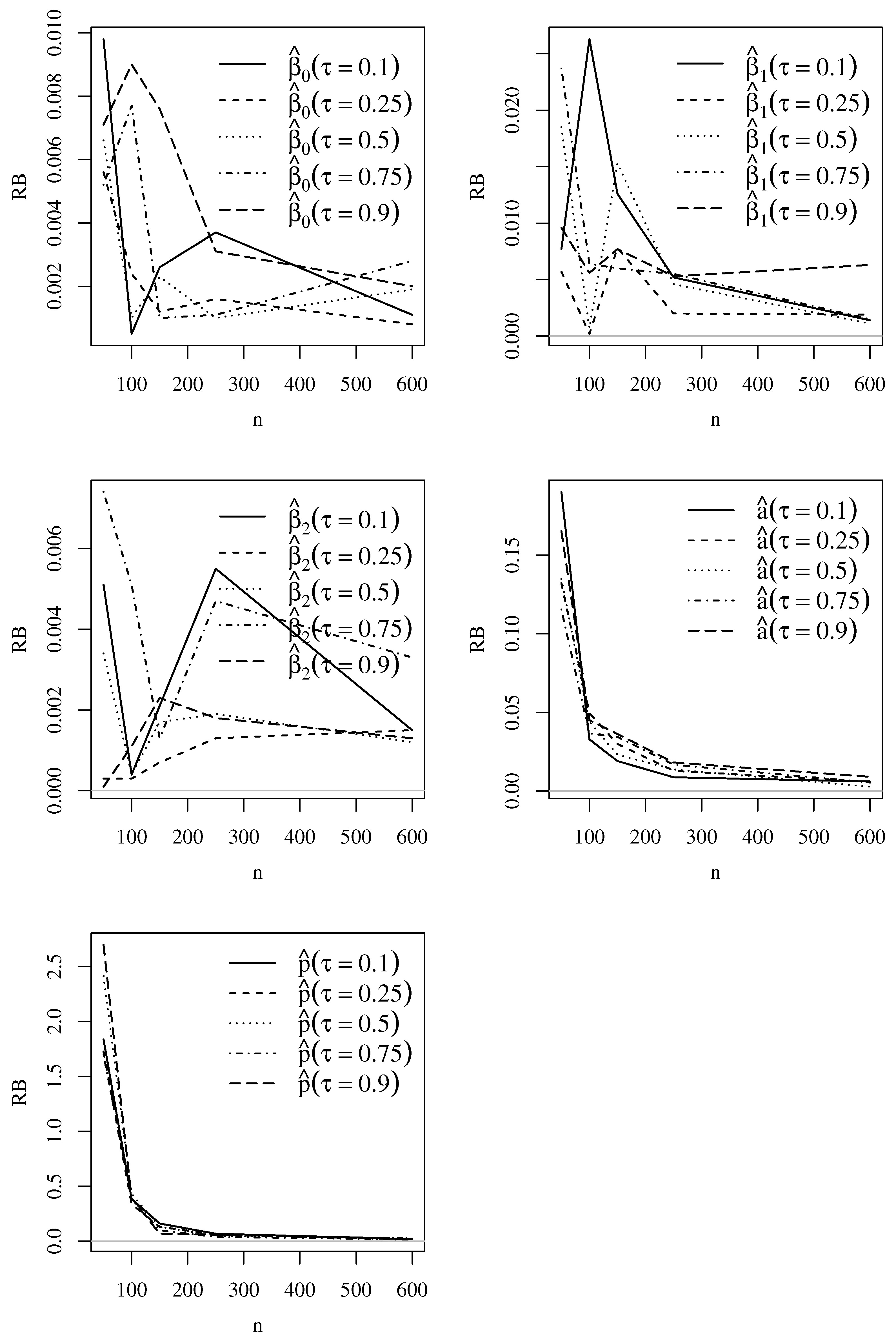
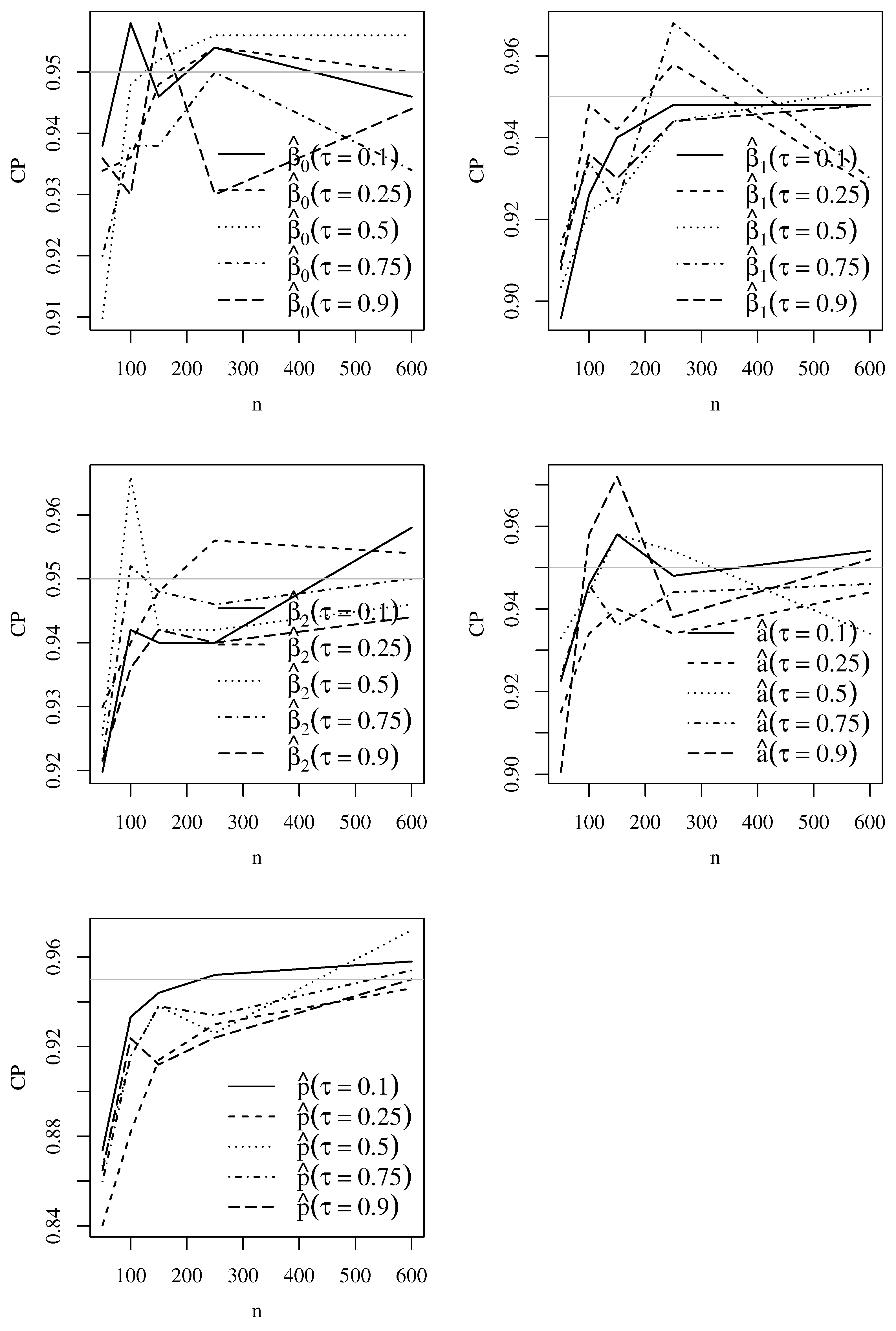
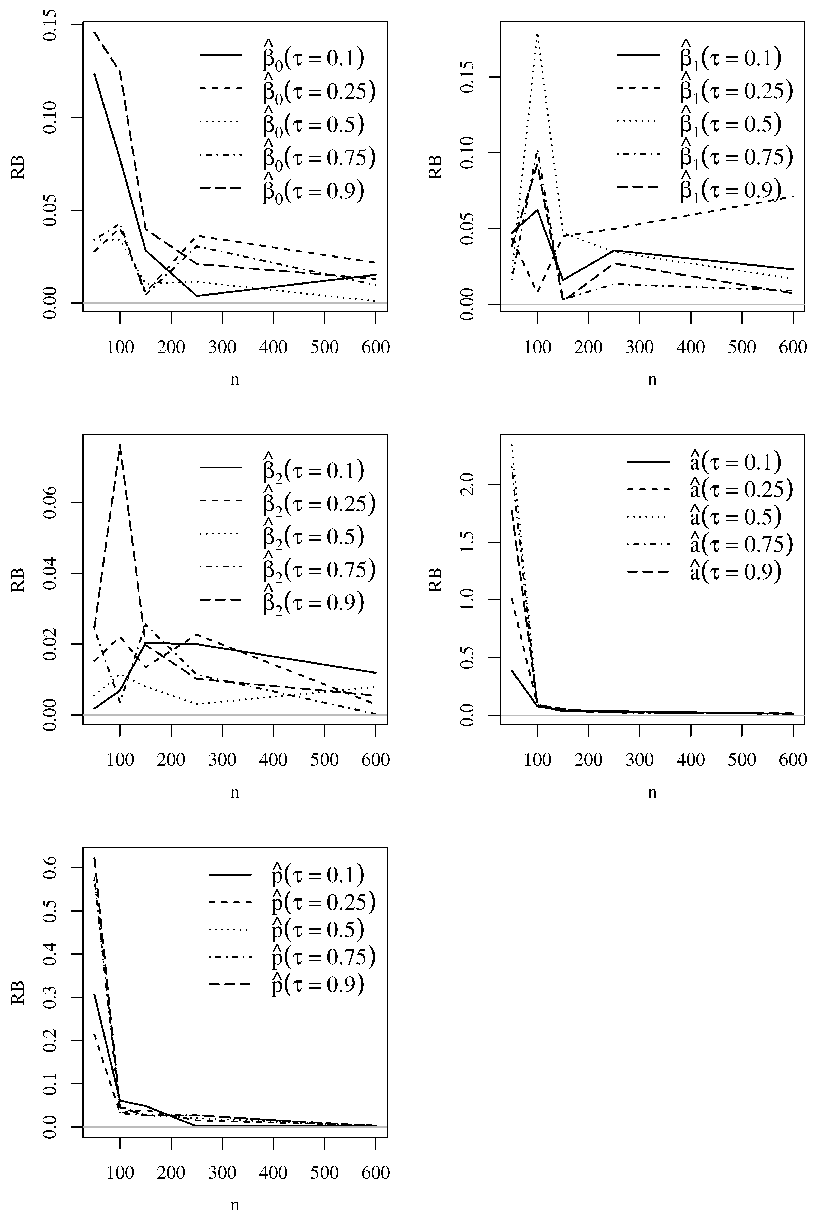
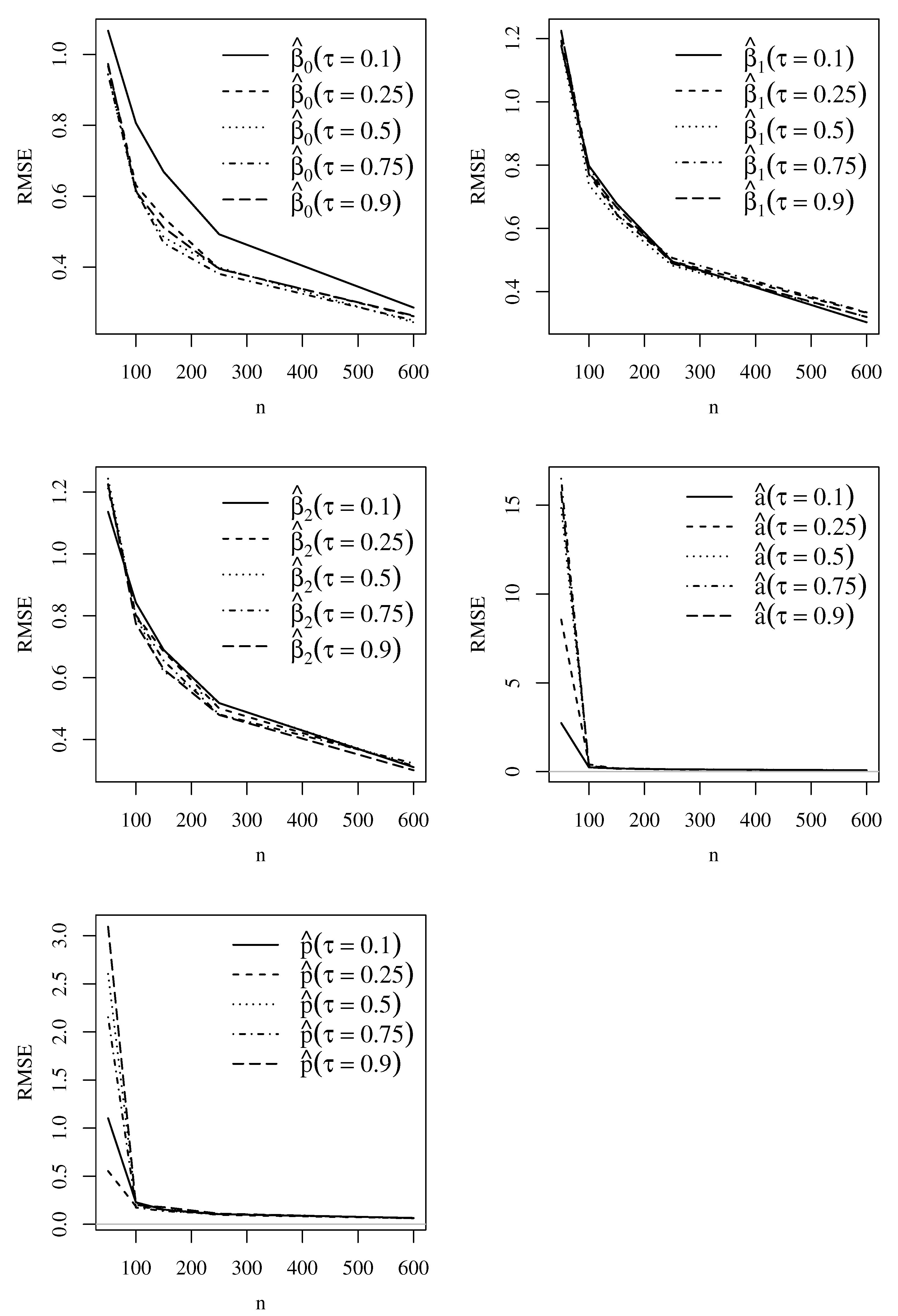
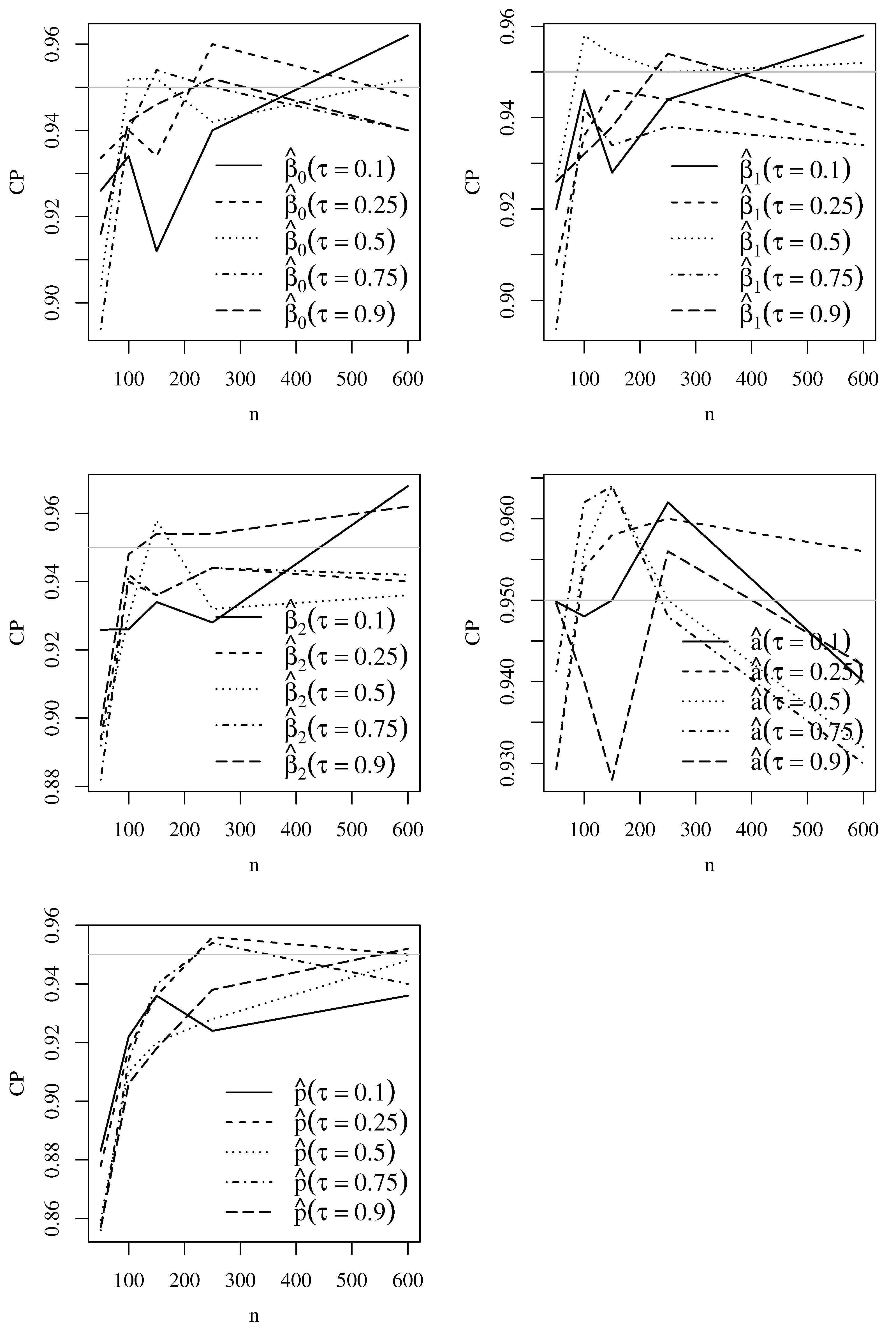
The Monte Carlo simulation experiments were performed using the R software; see www.r-project.org, accessed on 9 January 2023. The simulation scenario considers the following settings: sample sizes n { 50 , 100 , 150 , 250, 600 } , regression coefficients β ( τ ) = ( 1 , 0.5 , 1.5 ) , quantiles τ { 0.10 , 0.25 , 0.50 , 0.75 , 0.90 } , ( a , q ) = ( 5 , 1 ) for the Singh–Maddala model, and ( a , p ) = ( 1 , 0.5 ) for the Dagum model, with 500 Monte Carlo replications for each sample size. Covariate values x 1 i , x 2 i are obtained from a uniform distribution in the interval (0, 1). To study the ML estimators, we compute the relative bias (RB), root of the mean square error (RMSE), and coverage probability (CP). We expect that, as the sample size increases, the RB and RMSE reduce, and the CP approaches the 95% nominal level. The empirical RB, RMSE, and CP are computed from the Monte Carlo replications as
RB ^ ( θ ^ ) = 1 m i = 1 m θ ^ ( i ) θ θ , RMSE ^ ( θ ^ ) = 1 m i = 1 m ( θ ^ ( i ) θ ) 2 1 2 , CP ^ ( θ ^ ) = 1 m i = 1 m 1 { θ S } ,
where S [ L θ ^ ( i ) , U θ ^ ( i ) ] , θ and θ ^ ( i ) are the true parameter value and its respective i-th ML estimate, m is the number of Monte Carlo replications, 1 is as mentioned the indicator function taking the value 1 if θ [ L θ ^ ( i ) , U θ ^ ( i ) ] , and 0 otherwise, where L θ ^ ( i ) and U θ ^ ( i ) are the i-th lower and upper limits of the 95% confidence interval, respectively.
Empirical RB, RMSE, and CP values based on Monte Carlo simulations for the Singh–Maddala model parameters with a = 5 and q = 1 are shown in Figure 2, Figure 3 and Figure 4, whereas Figure 5, Figure 6 and Figure 7 display these values for the Dagum model parameters with a = 5 and p = 0.5 . Note that the simulations produced the expected outcomes. As the sample size increases, the RB and RMSE decrease, and the CP tends to 95%. The figures present results similar to those found for both Singh–Maddala and Dagum models.
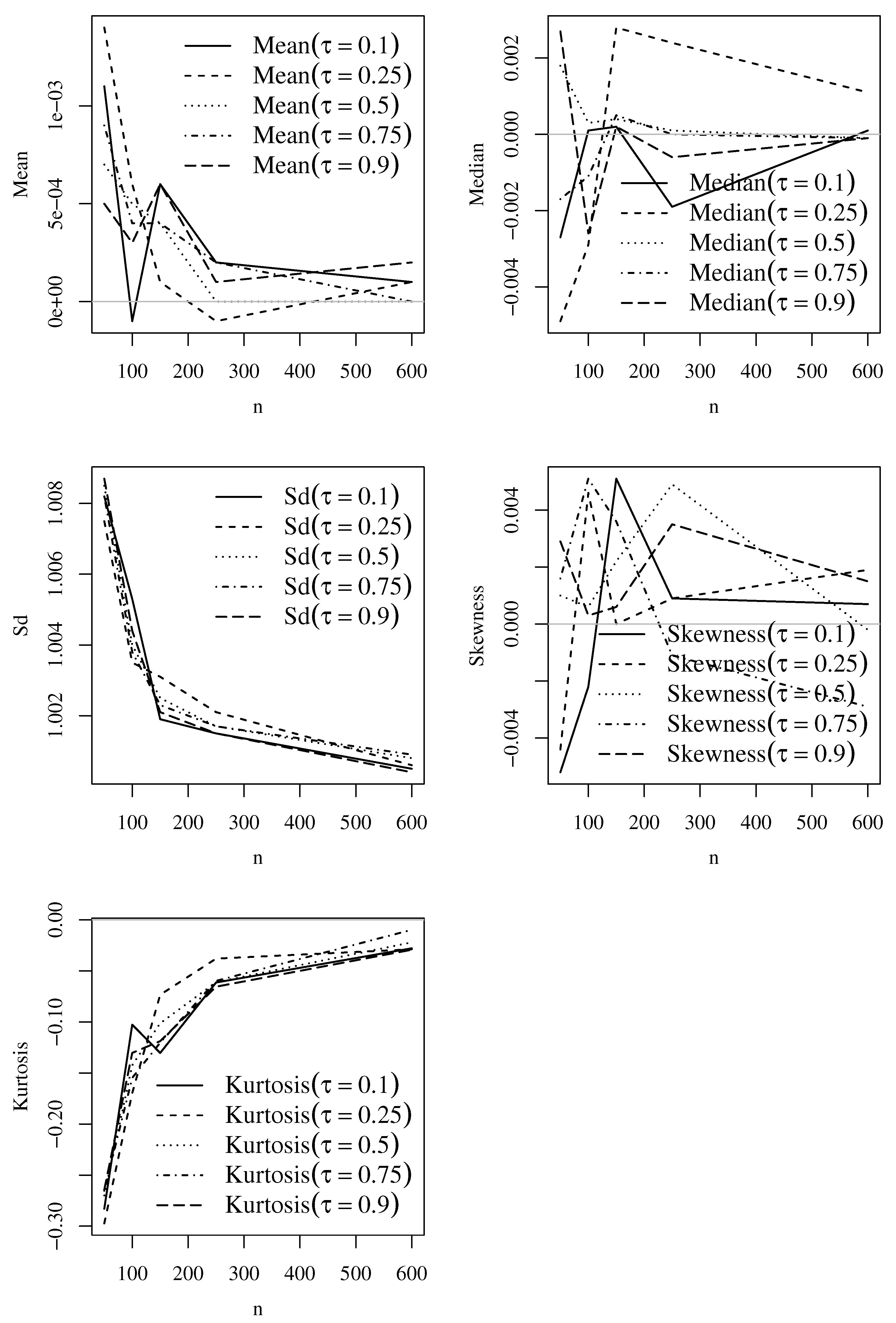
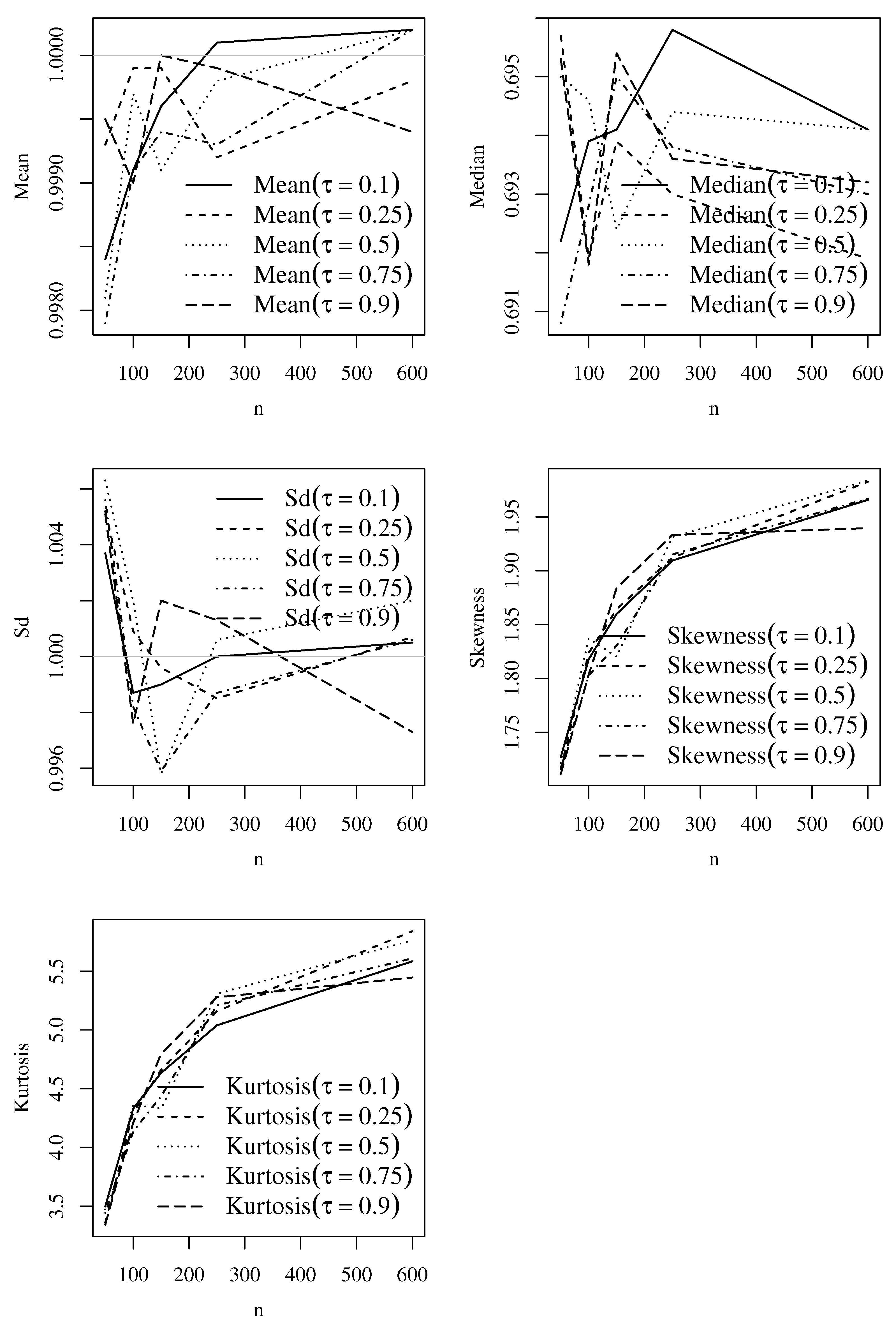
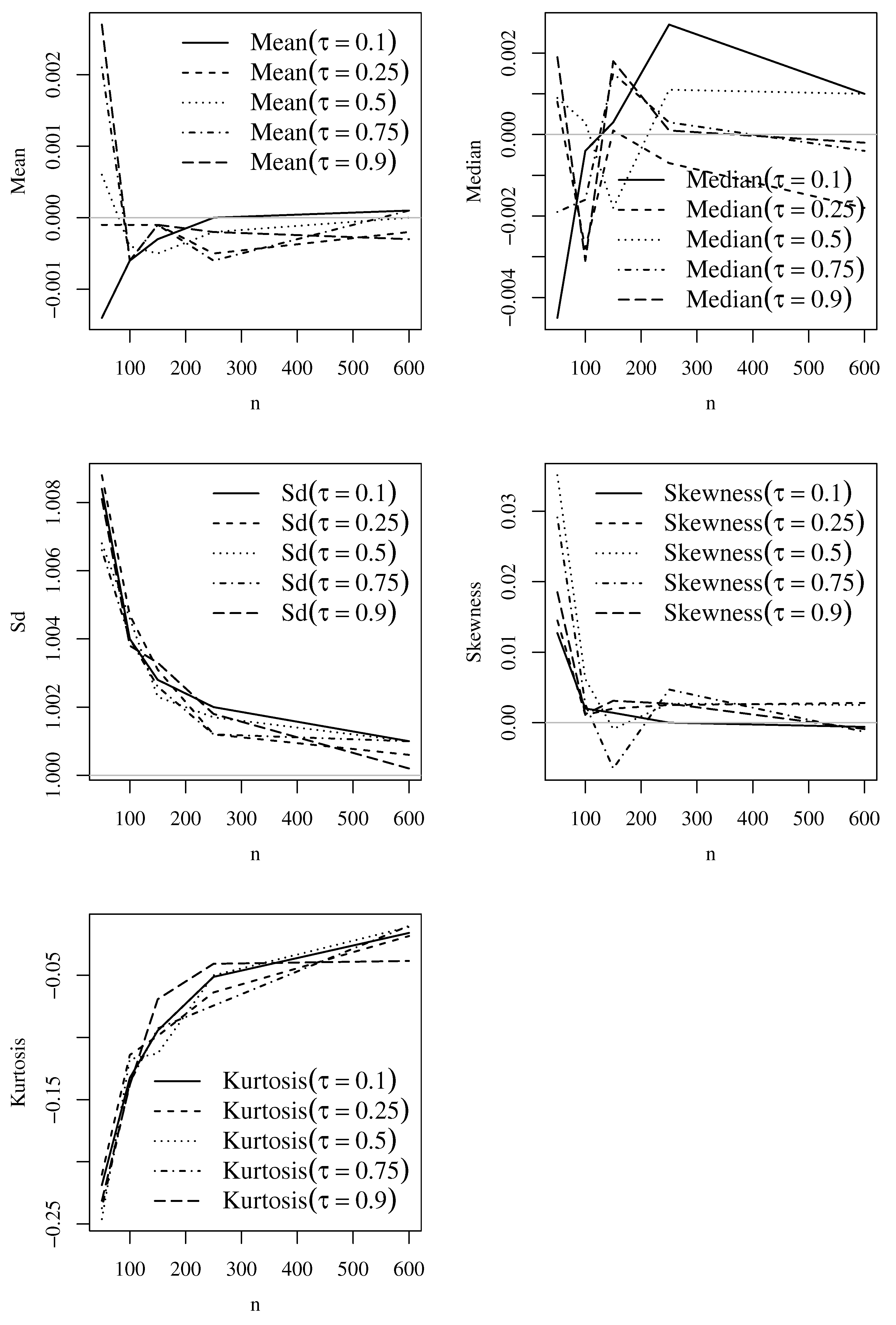
Next, we analyze the performance of GCS and RQ residuals with the sample mean, median, standard deviation (Sd), coefficient of skewness, and coefficient of kurtosis. Figure 8, Figure 9, Figure 10 and Figure 11 show empirical statistical indicators based on Monte Carlo simulations of the GCS and RQ residuals of the Singh–Maddala and Dagum models. The reference values of mean, median, Sd, skewness, and kurtosis are 1, 0.69, 1, 2, and 6, respectively, for the GCS residuals, and 0, 0, 1, 0, and 0, respectively, for the RQ residuals. From these figures, note that, as the sample size increases, the values tend to the expected results for each τ . Then, we will use both residuals to verify the fit of our models to income data.

4. Application to Income Data

In this section, we model income real data via parametric quantile regressions.

4.1. Data Set and Variables

We use the 2016 Chilean household income data set, provided by the National Institute of Statistics in Chile (available at www.ine.cl/estadisticas/sociales/ingresos-y-gastos/encuesta-suplementaria-de-ingresos, accessed on 9 January 2023), to illustrate the proposed parametric quantile regression models. This data set was also used in [37], which introduced the Birnbaum–Saunders quantile regression model. While the Birnbaum–Saunders model is not a distribution commonly used for income data [43,44,45,46,47], the Singh–Maddala and Dagum distributions are. Then, we assess if these models can produce better fits than the Birnbaum–Saunders model.
The household income is the response variable (Y). In contrast, the covariates are the total income due to salaries ( X 1 ), the total income due to independent work ( X 2 ), and the total income due to retirements ( X 3 ). The original dataset contains 107 variables, including those mentioned above. The variables were selected based on economic and statistical criteria concerning the response and descriptive analysis conducted in [37]. Moreover, all incomes are expressed in thousands of Chilean pesos (see www.bcentral.cl for their equivalence in American dollars, accessed on 9 January 2023).

4.2. Exploratory Data Analysis

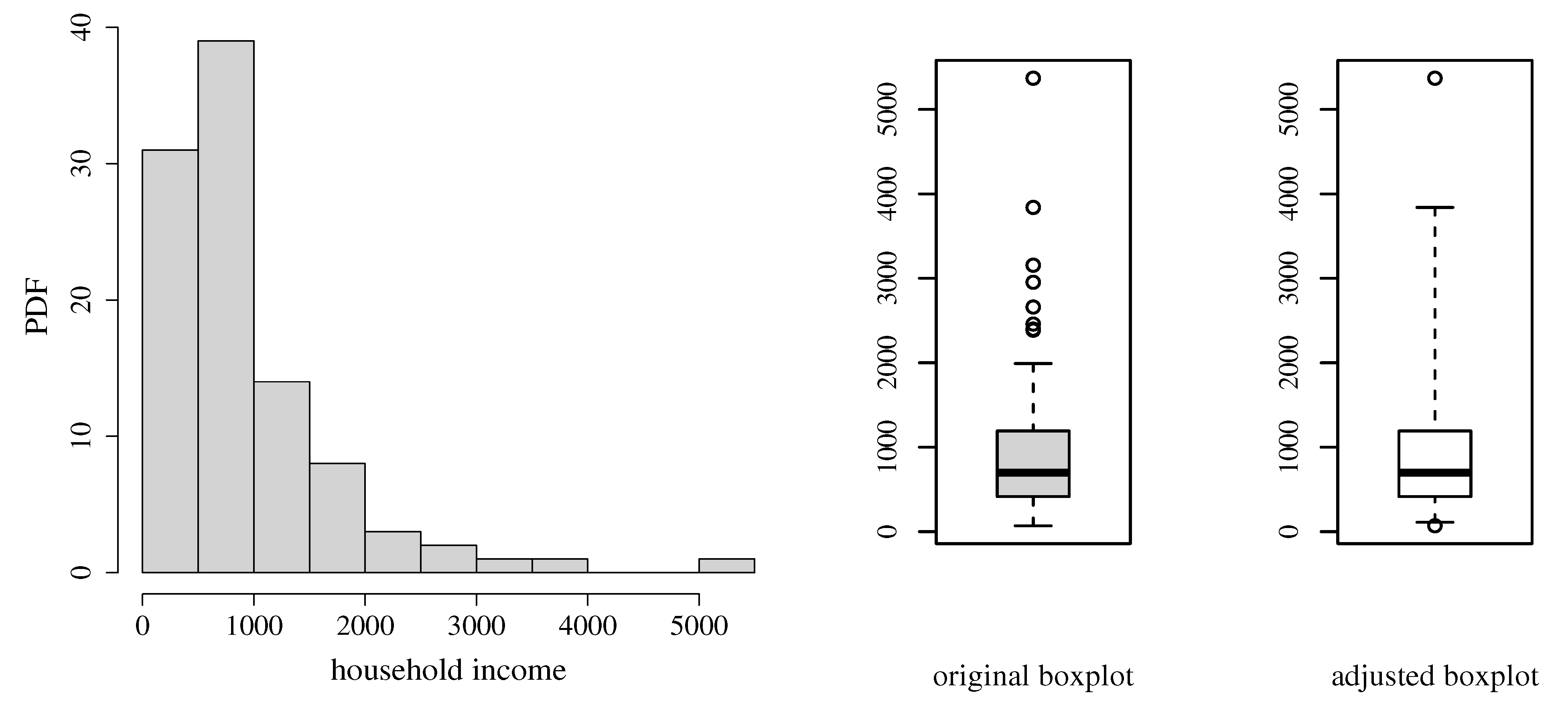
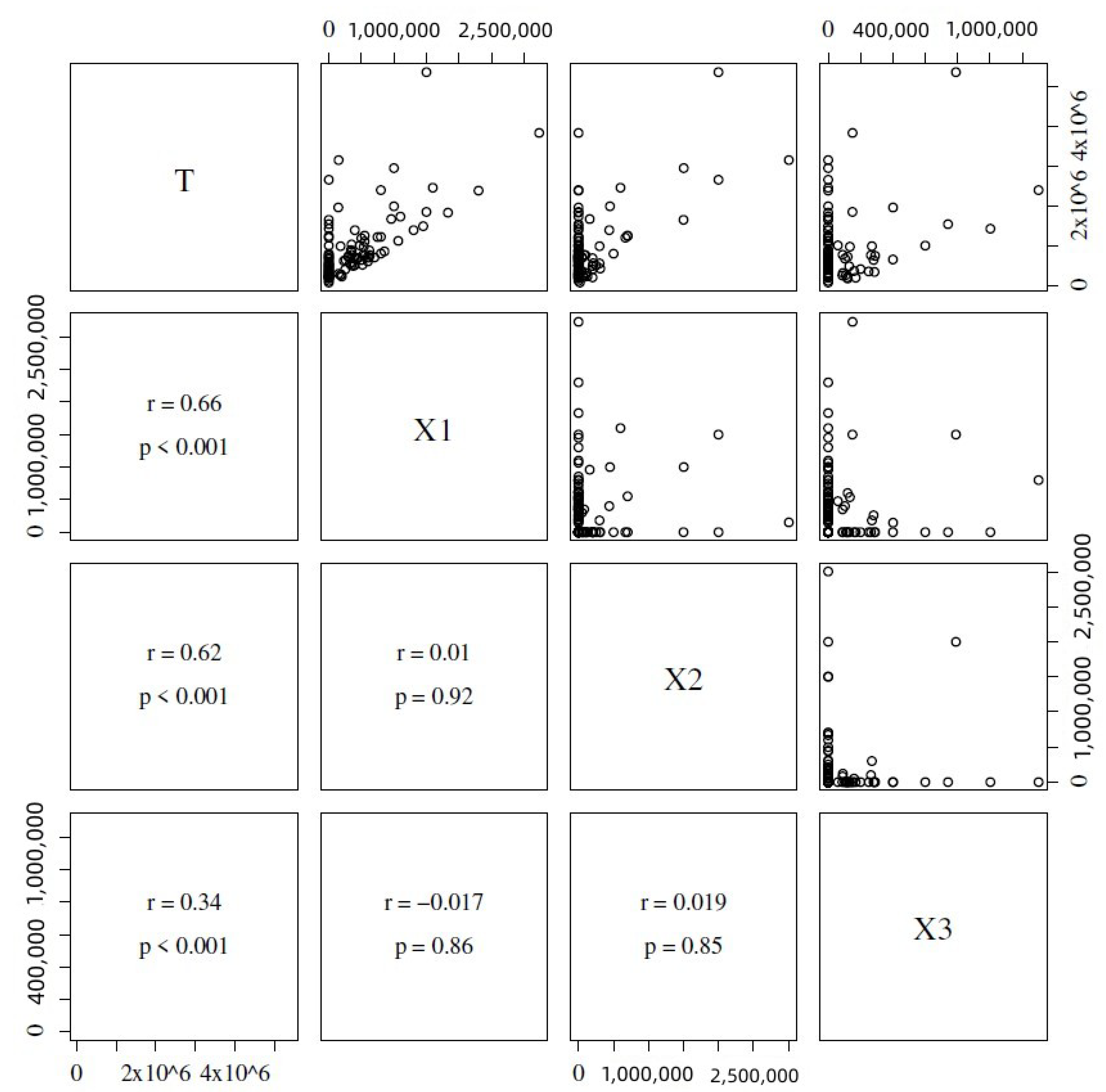
Table 2 reports descriptive statistics for the household income. Figure 12 shows the histogram along with usual and adjusted box plots [48]. Note that these income data have unimodal and right-skewed behavior, which is the needed scenario to use asymmetric distributions. Figure 13 shows scatterplots (with correlation) between the income Y and the covariates X 1 , X 2 , and X 3 . We observe that correlations are reasonable and significant when testing H 0 : ρ = 0 , where ρ is the correlation coefficient and r is the sample correlation. Meanwhile, the covariates have almost no linear correlation with each other.

4.3. Modeling

We then analyze the household income data using the Singh–Maddala and Dagum quantile regression models, with link structure expressed as (we use this specification to compare the results of the proposed models with those of the Birnbaum–Saunders quantile regression model)
γ i = β 0 ( τ ) + β 1 ( τ ) x 1 i + β 2 ( τ ) x 2 i + β 3 ( τ ) x 3 i , i { 1 , , 100 } .
The proposed models are fitted using the function IncomeReg.fit, implemented in the R software [49] by the authors. The codes are available upon request.
Table 3 presents the ML estimates, computed by the BFGS quasi-Newton method, standard errors (SEs) and Akaike (AIC) and Bayesian information (BIC) criteria values, for the Singh–Maddala and Dagum quantile regression models with τ = 0.50 . As mentioned earlier, the results of the Birnbaum–Saunders quantile regression are also presented. Table 3 reveals that the proposed Singh–Maddala and Dagum models provide better adjustments than the Birnbaum–Saunders model based on the values of log-likelihood, AIC, and BIC. Remarkably, the Singh–Maddala model has the minimum AIC and BIC values.
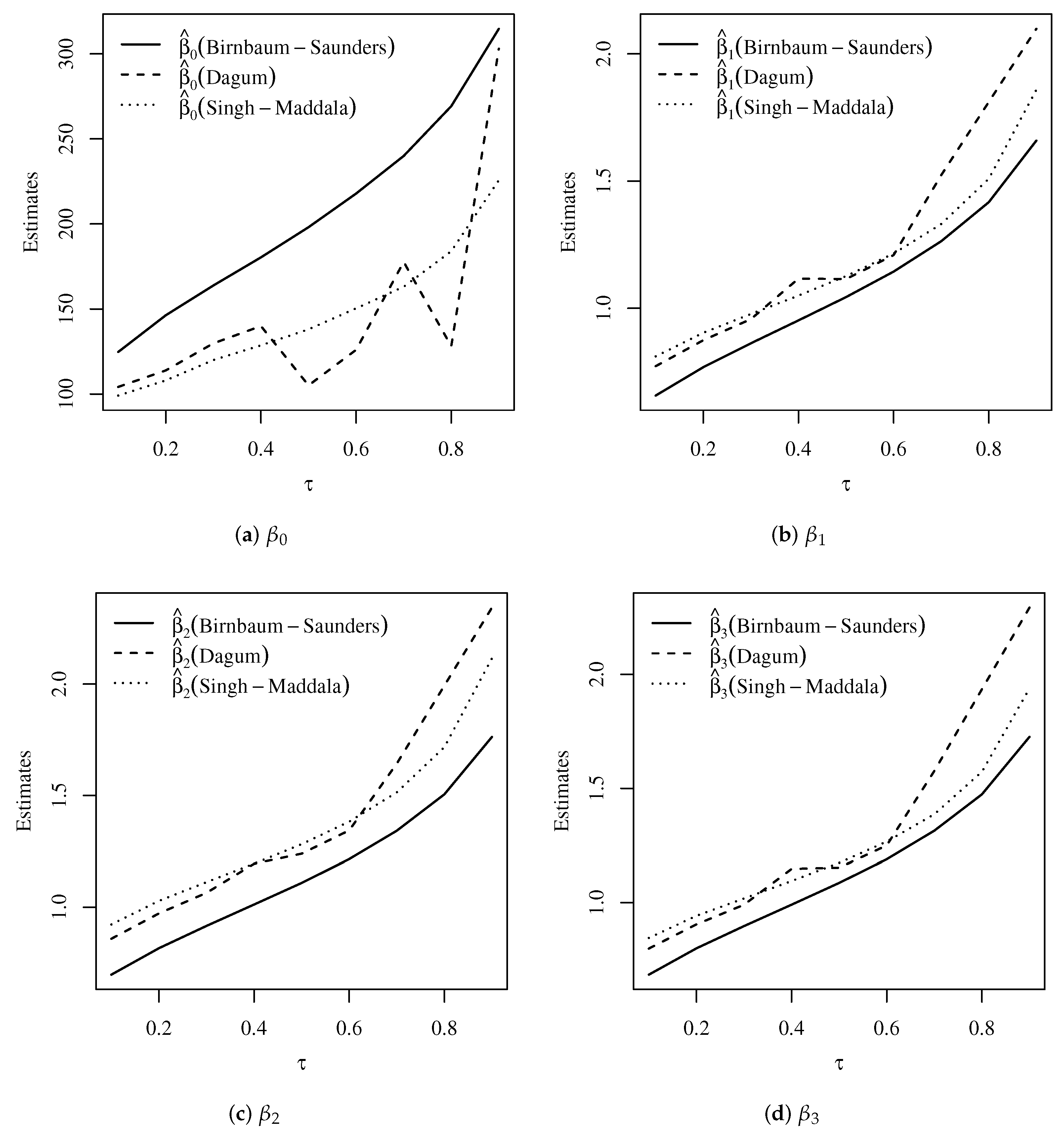
The estimated parameters of the Birnbaum–Saunders, Dagum, and Singh–Maddala models across τ are shown in Figure 14. From this figure, we observe that the estimates associated with all the covariates tend to increase as τ increases, as expected.
The QQ plots with a simulated envelope of the GCS and RQ residuals for the models considered in Table 3 confirm the results presented in Table 3; see Figure 15. Similar results are obtained when considering τ { 0.10 , , 0.90 } .
Figure 16 shows 95% prediction intervals from the Birnbaum–Saunders, Dagum, and Singh–Maddala quantile regression models for the household income data. The predictions were performed 20 steps ahead. Therefore, a total of 20 observations were not included in the estimation. From Figure 16, we observe that 95% of the observations are within the limits of the prediction interval for all the Birnbaum–Saunders, Dagum, and Singh–Maddala models. Therefore, all the models provide values closer to the nominal 95% level.

5. Concluding Remarks

5.1. Economic Statements

Quantile regression models permit a better analysis of household income, which can have different effects on socio-economic strata. Note that the covariates affect positively the household income, as expected. Note that the effects of all the covariates increase with the household income (higher quantiles) in our quantile regression model. For example, an increase of one thousand Chilean pesos in salaries ( X 1 ), increases the 50th percentile ( q = 0.50 ) of the household income by an amount of $1,125,200 Chilean pesos. As mentioned, see www.bcentral.cl (accessed on 9 January 2023) for the equivalence between Chilean pesos and American dollars. Note also that the estimated coefficient for the total income due to independent work ( X 2 ) in our quantile regression model for q = 0.5 is 1.2805. This suggests that an increase of one thousand Chilean pesos of income due to pensions provides an average increase of $1,280,500 in household income. Observe that the increase would not be substantial for most of the population. Similarly, the estimated coefficient for the total income due to retirements ( X 3 ) in our median regression model is 1.1730, which is greater than the corresponding estimated coefficient in the mean regression model. In general, we can conclude that economic analyses are more informative using quantile regression. In the present application, our quantile regression model provided a thorough tool to analyze income data.

5.2. Concluding Remarks

As mentioned, several parametric quantile regression models have been proposed in the literature considering diverse distributions [3,23,24,25,26,27,28,29,30,31,32,33,34,35]. The reader is referred to [36] for a full overview of parametric quantile regressions, their applications, and computational implementations, which are helpful to model indexes, proportions, and rates. However, to the best of our knowledge, parametric quantile regressions based on the Dagum and Singh–Maddala distributions were not considered until now.
In this article, we have proposed parametric quantile regression models based on the Singh–Maddala and Dagum distributions. The proposed models employed reparameterizations of the original distributions by including the quantile as a parameter. The maximum likelihood method was used to estimate the model parameters. Monte Carlo simulation studies were conducted to evaluate the estimators’ performance and the empirical distribution of the generalized Cox–Snell and randomized quantile residuals. The results empirically showed that the estimators had an excellent performance, and the residuals presented a good agreement with their reference distributions. We applied the proposed models to a real data set by modeling the household income as a function of the following covariates: total income due to salaries, total income due to independent work, and total income due to retirement. The results were compared to the Birnbaum–Saunders quantile regression model. We showed that both Singh–Maddala and Dagum models have a better fit to data than the Birnbaum–Saunders model, with the Singh–Maddala model also showing a slightly superior performance than the Dagum model. Therefore, the results favored the use of the Singh–Maddala and Dagum quantile regression models.

5.3. Further Investigation

Covariates may have an effect on the quantiles as well as on the shape parameter. Based on [50], the joint effect that the covariates may have on both quantiles and the shape parameter in a regression modeling should be studied. In addition, we plan to analyze formulations of the model derived in the present investigation under multivariate, spatial, temporal, and partial least squares structures [44,51,52,53,54,55,56,57,58]. Furthermore, econometrical formulations may be assumed for the quantile regression model analyzed in the present study [59,60,61]. Moreover, the use of censored data and reliability models can also be of interest to be analyzed [38,45] as well as control charts for quantiles based on covariates [62]. We are planning to conduct studies on these issues in the future.

Author Contributions

Data curation: H.S., R.V., G.V.B. and M.B.; formal analysis: H.S., R.V., G.V.B., M.B., V.L. and C.M.; investigation: H.S., R.V., G.V.B., M.B., V.L. and C.M.; methodology: H.S., R.V., G.V.B., M.B., V.L. and C.M.; writing—original draft: H.S., R.V., G.V.B., M.B. and C.M.; writing—review and editing: V.L. All authors have read and agreed to the published version of the manuscript.

Funding

This study was funded by CNPq grant number 309674/2020-4 (H.S.) from the Brazilian government, and by FONDECYT grant number 1200525 (V.L.) and FONDECYT grant number 1190636 (C.M.) from the National Agency for Research and Development (ANID) of the Chilean government under the Ministry of Science, Technology, Knowledge, and Innovation.

Data Availability Statement

Not applicable.

Acknowledgments

The authors would also like to thank the reviewers for their constructive comments which led to improvement in the presentation of the manuscript.

Conflicts of Interest

The authors declare that they have no conflict of interest.

References

  1. Galarza, C.E.; Zhang, P.; Lachos, V.H. Logistic quantile regression for bounded outcomes using a family of heavy-tailed distributions. Sankhya B 2021, 83, 325–349. [Google Scholar] [CrossRef]
  2. Sánchez, L.; Leiva, V.; Saulo, H.; Marchant, C.; Sarabia, J.M. A new quantile regression model and its diagnostic analytics for a Weibull distributed response with applications. Mathematics 2021, 9, 2768. [Google Scholar] [CrossRef]
  3. Saulo, H.; Dasilva, A.; Leiva, V.; Sánchez, L.; Fuente-Mella, H.L. Log-symmetric quantile regression models. Stat. Neerl. 2021, 76, 124–163. [Google Scholar] [CrossRef]
  4. Haupt, H.; Fritsch, M. Quantile trend regression and its application to central England temperature. Mathematics 2022, 10, 413. [Google Scholar] [CrossRef]
  5. Shin, K.; You, S. Quantile regression analysis between the after-school exercise and the academic performance of Korean middle school students. Mathematics 2021, 10, 58. [Google Scholar] [CrossRef]
  6. Koenker, R. Quantile Regression; Cambridge University Press: Cambridge, UK, 2005. [Google Scholar]
  7. Pareto, V. Cours d’éEonomie Politique; Librairie Droz: Paris, France, 1897; Volume 1. [Google Scholar]
  8. Reed, W.J. The Pareto law of incomes—An explanation and an extension. Phys. A Stat. Mech. Its Appl. 2003, 319, 469–486. [Google Scholar] [CrossRef]
  9. Shirras, G.F. The Pareto law and the distribution of income. Econ. J. 1935, 45, 663–681. [Google Scholar] [CrossRef]
  10. Johnson, N.L.; Kotz, S.; Balakrishnan, N. Continuous Univariate Distributions; Wiley: New York, NY, USA, 1995; Volume 2. [Google Scholar]
  11. Kotz, S.; Leiva, V.; Sanhueza, A. Two new mixture models related to the inverse Gaussian distribution. Methodol. Comput. Appl. Probab. 2010, 12, 199–212. [Google Scholar] [CrossRef]
  12. Cramer, J.S. Empirical Econometrics; North-Holland: Amsterdam, The Netherlands, 1971. [Google Scholar]
  13. Dagum, C. A new model of personal income distribution: Specification and estimation. In Modeling Income Distributions and Lorenz Curves; Springer: New York, NY, USA, 2008; pp. 3–25. [Google Scholar]
  14. Dagum, C. Un modèle Nonlinéaire de Répartition Fonctionnelle du Revenu; Department of Economical Sciences, University of Ottawa: Ottawa, ON, Canada, 1973. [Google Scholar]
  15. Dagum, C. A model of income distribution and the conditions of existence of moments of finite order. Bull. Int. Stat. Inst. 1975, 46, 199–205. [Google Scholar]
  16. Elbatal, I.; Aryal, G. Transmuted Dagum distribution with applications. Chil. J. Stat. 2015, 6, 31–45. [Google Scholar]
  17. Kleiber, C. A guide to the Dagum distributions. In Modeling Income Distributions and Lorenz Curves; Springer: New York, NY, USA, 2008; pp. 97–117. [Google Scholar]
  18. Krämer, W.; Ziebach, T. The Weak Pareto Law and Regular Variation in the Tails; Technical Report; University of Dortmund: Dortmund, Germany, 2002. [Google Scholar]
  19. Singh, S.; Maddala, G.S. A function for size distribution of incomes. In Modeling Income Distributions and Lorenz Curves; Springer: New York, NY, USA, 2008; pp. 27–35. [Google Scholar]
  20. Kumar, D. The Singh-Maddala distribution: Properties and estimation. Int. J. Syst. Assur. Eng. Manag. 2017, 8, 1297–1311. [Google Scholar] [CrossRef]
  21. Hajargasht, G.; Griffiths, W.E.; Brice, J.; Rao, D.P.; Chotikapanich, D. Inference for income distributions using grouped data. J. Bus. Econ. Stat. 2012, 30, 563–575. [Google Scholar] [CrossRef]
  22. Kleiber, C. Dagum vs. Singh-Maddala income distributions. Econ. Lett. 1996, 53, 265–268. [Google Scholar] [CrossRef]
  23. Jodrá, P.; Jiménez-Gamero, M.D. A quantile regression model for bounded responses based on the exponential-geometric distribution. REVSTAT—Stat. J. 2020, 4, 415–436. [Google Scholar]
  24. Korkmaz, M.Ç.; Chesneau, C. On the unit Burr-XII distribution with the quantile regression modeling and applications. Comput. Appl. Math. 2021, 40, 29. [Google Scholar] [CrossRef]
  25. Korkmaz, M.Ç.; Chesneau, C.; Korkmaz, Z.S. A new alternative quantile regression model for the bounded response with educational measurements applications of OECD countries. J. Appl. Stat. 2023, 50, 131–154. [Google Scholar] [CrossRef]
  26. Korkmaz, M.Ç.; Chesneau, C.; Korkmaz, Z.S. On the arcsecant hyperbolic normal distribution. Properties, quantile regression modeling and applications. Symmetry 2021, 13, 117. [Google Scholar] [CrossRef]
  27. Korkmaz, M.Ç.; Chesneau, C.; Korkmaz, Z.S. Transmuted unit Rayleigh quantile regression model: Alternative to beta and Kumaraswamy quantile regression models. Univ. Politeh. Buchar. Sci. Bull. A Appl. Math. Phys. 2021, 83, 149–158. [Google Scholar]
  28. Korkmaz, M.Ç.; Emrah, A.; Chesneau, C.; Yousof, H.M. On the unit-Chen distribution with associated quantile regression and applications. Math. Slovaca 2021, 72, 765–786. [Google Scholar] [CrossRef]
  29. Korkmaz, M.Ç.; Korkmaz, Z.S. The unit log–log distribution: A new unit distribution with alternative quantile regression modeling and educational measurements applications. J. Appl. Stat. 2023. [Google Scholar] [CrossRef]
  30. Mazucheli, M.; Alves, B.; Korkmaz, M.C.; Leiva, V. Vasicek quantile and mean regression models for bounded data: New formulation, mathematical derivations, and numerical applications. Mathematics 2022, 10, 1389. [Google Scholar] [CrossRef]
  31. Mazucheli, M.; Korkmaz, M.C.; Menezes, A.F.B.; Leiva, V. The unit generalized half-normal quantile regression model: Formulation, estimation, diagnostics, and numerical applications. Soft Comput. 2023, 27, 279–295. [Google Scholar] [CrossRef] [PubMed]
  32. Saulo, H.; Vila, R.; Bittencourt, V.L.; Leao, J.; Leiva, V.; Christakos, G. On a new extreme value distribution: Characterization, parametric quantile regression, and application to extreme air pollution events. Stoch. Environ. Res. Risk Assess. 2023. [Google Scholar] [CrossRef]
  33. Mazucheli, J.; Leiva, V.; Alves, B.; Menezes, A.F.B. A new quantile regression for modeling bounded data under a unit Birnbaum-Saunders distribution with applications in medicine and politics. Symmetry 2021, 13, 682. [Google Scholar] [CrossRef]
  34. Mazucheli, J.; Menezes, A.F.B.; Fernandes, L.B.; de Oliveira, R.P.; Ghitany, M.E. The unit-Weibull distribution as an alternative to the Kumaraswamy distribution for the modeling of quantiles conditional on covariates. J. Appl. Stat. 2020, 47, 954–974. [Google Scholar] [CrossRef]
  35. Mazucheli, J.; Menezes, A.F.B.; Ghitany, M.E. The unit-Weibull distribution and associated inference. J. Appl. Probab. Stat. 2018, 13, 1–22. [Google Scholar]
  36. Mazucheli, M.; Alves, B.; Menezes, A.F.B.; Leiva, V. An overview on parametric quantile regression models and their computational implementation with applications to biomedical problems including COVID-19 data. Comput. Methods Programs Biomed. 2022, 221, 106816. [Google Scholar] [CrossRef] [PubMed]
  37. Sánchez, L.; Leiva, V.; Galea, M.; Saulo, H. Birnbaum-saunders quantile regression and its diagnostics with application to economic data. Appl. Stoch. Model. Bus. Ind. 2021, 37, 53–73. [Google Scholar] [CrossRef]
  38. Guiraud, P.; Leiva, V.; Fierro, R. A non-central version of the Birnbaum-Saunders distribution for reliability analysis. IEEE Trans. Reliab. 2009, 58, 152–160. [Google Scholar] [CrossRef]
  39. Klugman, S.A.; Panjer, H.H.; Willmot, G.E. Loss Models: From Data to Decisions; Wiley: New York, NY, USA, 2019. [Google Scholar]
  40. Gradshteyn, I.; Ryzhik, I. Table of Integrals, Series and Products; Academic Press: San Diego, CA, USA, 2015. [Google Scholar]
  41. Mittelhammer, R.C.; Judge, G.G.; Miller, D.J. Econometric Foundations Pack with CD-ROM; Cambridge University Press: Cambridge, UK, 2000. [Google Scholar]
  42. Cox, D.R.; Hinkley, D.V. Theoretical Statistics; CRC Press: Boca-Raton, FL, USA, 1979. [Google Scholar]
  43. Mazucheli, J.; Menezes, A.F.; Dey, S. The unit-Birnbaum-Saunders distribution with applications. Chil. J. Stat. 2018, 9, 47–57. [Google Scholar]
  44. Huerta, M.; Leiva, V.; Liu, S.; Rodriguez, M.; Villegas, D. On a partial least squares regression model for asymmetric data with a chemical application in mining. Chemom. Intell. Lab. Syst. 2019, 190, 55–68. [Google Scholar] [CrossRef]
  45. Leao, J.; Leiva, V.; Saulo, H.; Tomazella, V. Incorporation of frailties into a cure rate regression model and its diagnostics and application to melanoma data. Stat. Med. 2018, 37, 4421–4440. [Google Scholar] [CrossRef] [PubMed]
  46. Marchant, C.; Leiva, V.; Cavieres, M.F.; Sanhueza, A. Air contaminant statistical distributions with application to PM10 in Santiago, Chile. Rev. Environ. Contam. Toxicol. 2013, 223, 1–31. [Google Scholar] [PubMed]
  47. Mazucheli, J.; Bapat, S.R.; Menezes, A.F.B. A new one-parameter unit-Lindley distribution. Chil. J. Stat. 2020, 11, 53–67. [Google Scholar]
  48. Rousseeuw, P.; Croux, C.; Todorov, V.; Ruckstuhl, A.; Salibian-Barrera, M.; Verbeke, T.; Koller, M.; Maechler, M. Robustbase: Basic Robust Statistics. R Package Version 0.92-6. 2016. Available online: https://cran.r-project.org/web/packages/robustbase/index.html (accessed on 18 December 2022).
  49. R Core Team. R: A Language and Environment for Statistical Computing; R Foundation for Statistical Computing: Vienna, Austria, 2019. [Google Scholar]
  50. Ventura, M.; Saulo, H.; Leiva, V.; Monsueto, S. Log-symmetric regression models: Information criteria, application to movie business and industry data with economic implications. Appl. Stoch. Model. Bus. Ind. 2019, 35, 963–977. [Google Scholar] [CrossRef]
  51. Leiva, V.; Saulo, H.; Leao, J.; Marchant, C. A family of autoregressive conditional duration models applied to financial data. Comput. Stat. Data Anal. 2014, 79, 175–191. [Google Scholar] [CrossRef]
  52. Garcia-Papani, F.; Leiva, V.; Ruggeri, F.; Uribe-Opazo, M.A. Kriging with external drift in a Birnbaum-Saunders geostatistical model. Stoch. Environ. Res. Risk Assess. 2018, 32, 1517–1530. [Google Scholar] [CrossRef]
  53. Garcia-Papani, F.; Leiva, V.; Uribe-Opazo, M.A.; Aykroyd, R.G. Birnbaum-Saunders spatial regression models: Diagnostics and application to chemical data. Chemom. Intell. Lab. Syst. 2018, 177, 114–128. [Google Scholar] [CrossRef] [Green Version]
  54. Marchant, C.; Leiva, V.; Cysneiros, F.J.A.; Liu, S. Robust multivariate control charts based on Birnbaum-Saunders distributions. J. Stat. Comput. Simul. 2018, 88, 182–202. [Google Scholar] [CrossRef]
  55. Martinez, S.; Giraldo, R.; Leiva, V. Birnbaum-Saunders functional regression models for spatial data. Stoch. Environ. Res. Risk Assess. 2019, 33, 1765–1780. [Google Scholar] [CrossRef]
  56. Saulo, H.; Leao, J.; Leiva, V.; Aykroyd, R.G. Birnbaum-Saunders autoregressive conditional duration models applied to high-frequency financial data. Stat. Pap. 2019, 60, 1605–1629. [Google Scholar] [CrossRef] [Green Version]
  57. Leiva, V.; Sanchez, L.; Galea, M.; Saulo, H. Global and local diagnostic analytics for a geostatistical model based on a new approach to quantile regression. Stoch. Environ. Res. Risk Assess. 2020, 34, 1457–1471. [Google Scholar] [CrossRef]
  58. Sanchez, L.; Leiva, V.; Galea, M.; Saulo, H. Birnbaum-Saunders quantile regression models with application to spatial data. Mathematics 2020, 8, 1000. [Google Scholar] [CrossRef]
  59. Desousa, M.; Saulo, H.; Leiva, V.; Scalco, P. On a tobit-Birnbaum-Saunders model with an application to medical data. J. Appl. Stat. 2018, 45, 932–955. [Google Scholar] [CrossRef]
  60. Cysneiros, F.J.A.; Leiva, V.; Liu, S.; Marchant, C.; Scalco, P. A Cobb-Douglas type model with stochastic restrictions: Formulation, local influence diagnostics and data analytics in economics. Qual. Quant. 2019, 53, 1693–1719. [Google Scholar] [CrossRef]
  61. de la Fuente-Mella, H.; Rojas-Fuentes, J.L.; Leiva, V. Econometric modeling of productivity and technical efficiency in the Chilean manufacturing industry. Comput. Ind. Eng. 2020, 139, 105793. [Google Scholar] [CrossRef]
  62. Leiva, V.; dos Santos, R.A.; Saulo, H.; Marchant, C.; Lio, Y. Bootstrap control charts for quantiles based on log-symmetric distributions with applications to monitoring of reliability data. Qual. Reliab. Eng. Int. 2023, 39, 1–24. [Google Scholar] [CrossRef]
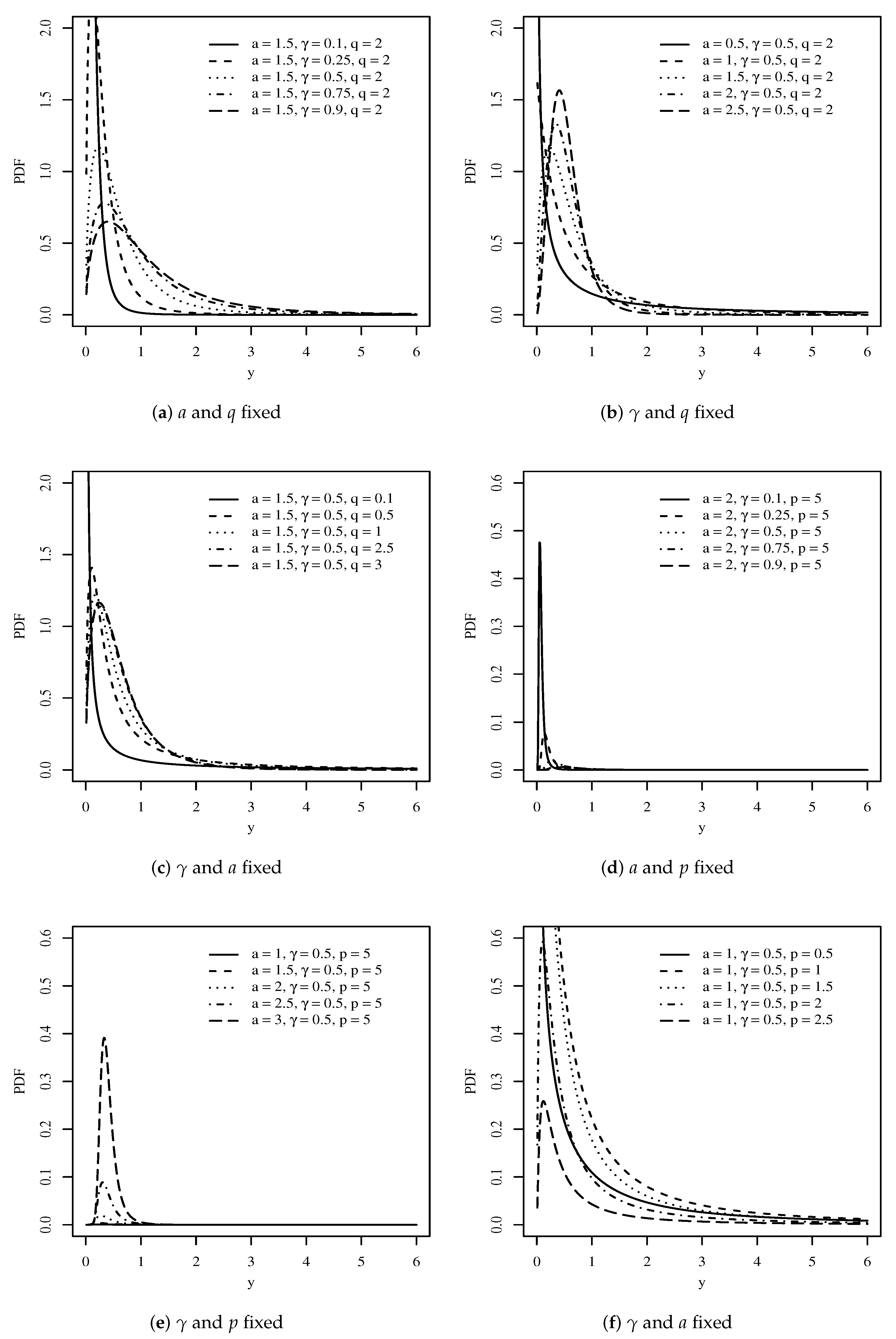
Figure 1. Quantile-based Singh–Maddala (ac) and Dagum (df) PDFs for the indicated values of the parameters. Source: data and own elaboration of the authors.
Mathematics 11 00448 g001
Figure 2. Plots of the empirical RB based on Monte Carlo simulation results for the indicated τ and Singh–Maddala model parameter with a = 5 and q = 1 . Source: data and own elaboration of the authors.
Mathematics 11 00448 g002
Figure 3. Plots of the empirical RMSE based on Monte Carlo simulation results for the indicated τ and Singh–Maddala model parameter with a = 5 and q = 1 . Source: data and own elaboration of the authors.
Mathematics 11 00448 g003
Figure 4. Plots of the empirical CP based on Monte Carlo simulation results for the indicated τ and Singh–Maddala model parameter with a = 5 and q = 1 . Source: data and own elaboration of the authors.
Mathematics 11 00448 g004
Figure 5. Plots of the empirical RB based on Monte Carlo simulation results for the indicated τ and Dagum model parameter with a = 5 and p = 0.5 . Source: data and own elaboration of the authors.
Mathematics 11 00448 g005
Figure 6. Plots of the empirical RMSE based on Monte Carlo simulation results for the indicated τ and Dagum model parameter with a = 5 and p = 0.5 . Source: data and own elaboration of the authors.
Mathematics 11 00448 g006
Figure 7. Plots of the empirical CP based on Monte Carlo simulation results for the indicated τ and Dagum model parameter with a = 5 and p = 0.5 . Source: data and own elaboration of the authors.
Mathematics 11 00448 g007
Figure 8. Plots of the listed statistical indicator based on Monte Carlo simulations of the GCS residuals for the Singh–Maddala model with a = 5 , q = 1 , and the indicated value of τ . Source: data and own elaboration of the authors.
Mathematics 11 00448 g008
Figure 9. Plots of the listed statistical indicator based on Monte Carlo simulations of the RQ residuals for the Singh–Maddala model with a = 5 , q = 1 , and the indicated value of τ . Source: data and own elaboration of the authors.
Mathematics 11 00448 g009
Figure 10. Plots of the listed statistical indicator based on Monte Carlo simulations of the GCS residuals for the Dagum model with a = 1 and p = 0.5 , and the indicated value of τ . Source: data and own elaboration of the authors.
Mathematics 11 00448 g010
Figure 11. Plots of the listed statistical indicator based on Monte Carlo simulations of the RQ residuals for the Dagum model with a = 1 and p = 0.5 , and the indicated value of τ . Source: data and own elaboration of the authors.
Mathematics 11 00448 g011
Figure 12. Histogram and boxplots for the household income data (in thousands of Chilean pesos). Source: data and own elaboration of the authors.
Mathematics 11 00448 g012
Figure 13. Scatterplots, sample Pearson correlations (r), and p-values of correlation ( ρ ) tests H 0 : ρ = 0 between variables Y , X 1 , X 2 , and X 3 . Source: data and own elaboration of the authors.
Mathematics 11 00448 g013
Figure 14. Plots of estimates for the indicated parameter (ad) and listed model across τ for the income data. Source: data and own elaboration of the authors.
Mathematics 11 00448 g014
Figure 15. QQ plot and its envelope for the indicated model and residual (af) for the income data ( τ = 0.50 ). Source: data and own elaboration of the authors.
Mathematics 11 00448 g015
Figure 16. 95% prediction intervals (20-steps-ahead) from the indicated model for the household income data. Source: data and own elaboration of the authors.
Mathematics 11 00448 g016
Table 1. PDF of the indicated income distribution for the traditional and quantile parameterizations.
DistributionTraditional PDF γ : τ -th QuantileSubstitutionQuantile-Based PDF
Singh–Maddala a q ( y / b ) a 1 b [ 1 + ( y / b ) a ] 1 + q γ = b c q 1 / a b = γ c q 1 / a a q c q ( y / γ ) a 1 γ [ 1 + c q ( y / γ ) a ] 1 + q
Dagum a p ( y / b ) a p 1 b [ 1 + ( y / b ) a ] 1 + p γ = b e p 1 / a b = γ e p 1 / a a p ( y / γ ) a p 1 γ e p p [ 1 + e p 1 ( y / γ ) a ] 1 + p
Table 2. Descriptive statistics for the household income data (in thousands of Chilean pesos).
MeanMedianSdCoefficient of VariationCoefficient of SkewnessCoefficient of KurtosisMinimumMaximumn
698.80938.10837.520.892.4511.03705369.90100
Table 3. ML estimate (with estimated SE in parenthesis) of the indicated parameter and model for the listed fitting measures using the income data.
ParameterBirnbaum–Saunders
( τ = 0.50 )
Dagum
( τ = 0.50 )
Singh–Maddala
( τ = 0.50 )
β 0 198.0903 *150.8307 *137.8478 *
(22.3166)(3.0771)( 3.2826)
β 1 1.0440 *1.1173 *1.1252 *
(0.0870)(0.0636)(0.0569)
β 2 1.1090 *1.2424 *1.2805 *
(0.1502)(0.1172)(0.1103)
β 3 1.0865 *1.1562 *1.1730 *
(0.1759)(0.1395)(0.1382)
α 0.3646 *
(0.0087)
a 4.37208.3380
(0.5692)(1.4720)
p or q 2.21000.4034
(1.0290)(0.1144)
Log-likelihood−692.8373−686.9182−685.2337
AIC1395.6751385.8361382.467
BIC1408.7011386.7401383.371
* significant at a level of 5%.
Disclaimer/Publisher’s Note: The statements, opinions and data contained in all publications are solely those of the individual author(s) and contributor(s) and not of MDPI and/or the editor(s). MDPI and/or the editor(s) disclaim responsibility for any injury to people or property resulting from any ideas, methods, instructions or products referred to in the content.