Prognostics and Health Management of the Robotic Servo-Motor under Variable Operating Conditions

Abstract

A robot is essential in many industrial and manufacturing facilities due to its efficiency, accuracy, and durability. However, continuous use of the robotic system can result in various component failures. The servo motor is one of the critical components, and its bearing is one of the vulnerable parts, hence failure analysis is required. Some previous prognostics and health management (PHM) methods are very limited in considering the realistic operating conditions of industrial robots based on various operating speeds, loading conditions, and motions, because they consider constant speed data with unloading conditions. This paper implements a PHM for the servo motor of a robotic arm based on variable operating conditions. Principal component analysis-based dimensionality reduction and correlation analysis-based feature selection are compared. Two machine learning algorithms have been used to detect fault features under various operating conditions. This method is proposed as a robust fault-detection model for industrial robots under various operating conditions. Features from different domains not only improved the generalization of the model’s performance but also improved the computational efficiency of massive data by reducing the total number of features. The results showed more than 90% accuracy under various operating conditions. As a result, the proposed method shows the possibility of robust failure diagnosis under various operating conditions similar to the actual industrial environment.

1. Introduction

With the development of the smart industry, robots, especially robotic arms, are being used in various applications, such as commercial fields and multi-robot cooperative systems. Therefore, the significance of robots is also increasing. A robot is essential in many industrial facilities due to its efficiency, accuracy, and durability [1,2].

One of the main components that comprise the robot is the servo motor, which determines the rated load and accuracy of the rotation angle of the robot. In particular, a servo motor is commonly used in industrial robots due to its high torque, small size, and precision control [3]. However, robots have many failure issues due to high torque, transformation stress, cyclic load, and impact load. After a certain period of operation, various failures such as bearing failure, broken rotor bars, and misalignment can occur. These failures cause production accidents and reduce productivity. Furthermore, if one of the robot components fails, the entire robot and production may suffer from unexpected expenses [4,5,6]. In this study, we deal with a fault that causes the major failure in 40% of all motor failures [7].

Prognostics and health management (PHM) can be used to detect or prevent such failures [1,8,9,10]. For PHM, the most representative techniques are ferrography analysis, acoustic emission analysis, vibration analysis, and motor current signature analysis (MCSA) [11]. However, in the case of vibration analysis and acoustic emission analysis, additional sensor installation is required. These additional sensors will complicate the system and incur additional costs. Besides, in the case of ferrography analysis, grease samples can be extracted directly from the reducer surface, and only internal structural defects can be diagnosed. In addition, real-time monitoring is difficult to achieve [5]. Therefore, MCSA can be used for real-time PHM without installing the extra sensors. The advantage of MCSA is that it can acquire real-time data by adding a current sensor to the electric circuit without having to attach a sensor to the device for fault diagnosis [5,12,13,14].

A PHM for motors based on constant speed scenarios is proposed in Reference [13]. However, in actual industrial applications, the robotic motor usually operates at variable speeds, and it is impractical to detect the constant speed of the robot’s motion for fault detections. Therefore, it is very important to consider the real industrial environment of varying operational speed with acceleration and deceleration [11]. Thus, research has been developed on robot motors with acceleration and deceleration under various speeds [5]. In addition, since the robot arm can operate under various loading conditions, one study detects failure by applying various loads to the motor with constant speed [15]. On the other hand, the robot operates with various motions, i.e., simple motions and complicated motions. Research and fault detection on the various motions of the robot has been conducted [14]. However, the same is not true for robust fault diagnosis studies of the various operating conditions mentioned. Therefore, various operating conditions such as speed, motions, and loads should be considered for robust fault detection.

In this study, a PHM approach for a robotic servo motor is proposed based on feature selection and reduction methods under varying operating conditions. In addition to time domain features and frequency domain features, the time–frequency domain was decomposed using the wavelet packet decomposition (WPD) method for feature extraction. Then, dimension reduction through principal component analysis (PCA) or feature selection through correlation analysis based on the Pearson coefficient are used to reduce the number of features and develop a machine learning algorithm. After the case study, the classifier is developed through two different machine learning algorithms in order to detect robust defect features for different operating conditions [16,17,18]. In order to develop a robust model under various operating conditions, we propose a model using features in different domains such as time, frequency, and combined time–frequency. The proposed approach is applicable under variable working conditions of motion, speed, and loading, which mimics real environmental scenarios. The generalization of the algorithms is validated in terms of two different ML classifiers. The computational cost is reduced by using feature selection techniques.

This paper is broken up into five sections. In Section 2, the methodology, which is composed of feature extraction, feature reduction, feature selection, and classification, is discussed. In Section 3, the experimental setup is described with detailed descriptions of the data used in the experiments and an explanation of the faulty conditions. Section 4 is composed of the results and discussions of this work. Finally, in Section 5, the conclusions of the proposed method are discussed.

2. Materials and Methods

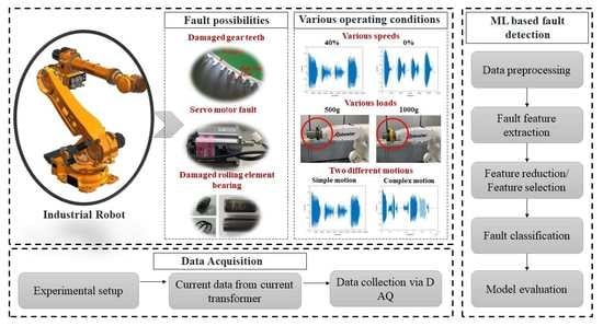
The proposed research work is shown in Figure 1. The first step is data acquisition and preprocessing. The current signal data is collected from the robot servo-motor. After a short-term Fourier transform (STFT), the continuous signal data is segmented at each cycle when the error between the sampled data and the original data is less than a criterion. After data preprocessing, features are extracted from the normalized signal. Extracting different features such as variance, standard deviation, and skewness from a signal is a common method proposed for fault detection [16,17]. However, due to the sheer volume of features, applying a classification algorithm can be time-consuming. In order to avoid such problems, feature reduction and feature selection methods are used for comparison to reduce the amount of computation. This technique is often used to avoid excessive complexity in the classification model. Among these dimension-reduction methods, PCA can be used to reduce the feature dimension and algorithm computation [18]. Also, in the feature selection method, correlation analysis is used to calculate the linear relationship between two features based on the Pearson correlation coefficient. When features with high linear correlation are determined to be equal, the number of features can be reduced by canceling them [19]. Finally, the classification performance is compared using ANN and SVM. The proposed method used a laboratory-scale experimental test bench to implement Robostar’s industrial, vertically articulated 6-axis robot. To detect servo-motor faults, current data are collected for normal and fault conditions. A fault is induced in the bearing of the motor. These defects are considered at the third axis of the robot.

2.1. Data Acquisition

The current signal is acquired from the robot servo motor through a current transformer and data acquisition module. Since the collected data is a continuous signal, the signal is divided into cycles in order to determine the fault feature in each cycle. Signal pre-processing is essential for the real-time fault detection of robot servo motors. In contrast to continuous incoming signals, preprocessing is required to separate the signal into one cycle from the original signal in order to analyze the failure of one cycle of the robot. For this purpose, the following process was carried out.

2.2. Data Pre-Processing

An arbitrary cycle was set as the model cycle in the original data. The original data and sample cycle were transformed using STFT. The original data with the length of the sample cycle were compared with the STFT value of the sample cycle, and the data were separated based on the minimum points where the error falls below the reference value. With this function, the signal can be separated into each cycle from the original signal that repeats itself. Figure 2 shows an example of signal segmentation.

2.3. Feature Extraction

A number of methods have been proposed to analyze faulty features. Among them, statistical features, sinusoidal wave shape-based features, and kinetic energy (KE)-based features were extracted in the time domain, and frequency domain features and time-frequency domain features were extracted. The feature extraction methods are described in

Table 1. Extracted features in different domains.

Domain	Features	Definition
Time domain	Sum [20]	$I_{sum}={\displaystyle \sum }_{k=1}^N\left(x\left(k\right)\right)$
	Variance [19]	$I_{var}=\raisebox{1ex}{$1$}\!\left/ \!\raisebox{-1ex}{$N$}\right.{\displaystyle \sum }_{k=1}^N\left(x\left(k\right)-I_{mean}\right)$
	Standard deviation [19]	$I_{std}=\sqrt{I_{var}}$
	Root mean square [21]	$I_{RMS}=\sqrt{\raisebox{1ex}{$1$}\!\left/ \!\raisebox{-1ex}{$N$}\right.{\displaystyle \sum }_{k=1}^N{\left(x\left(k\right)\right)}^2}$
	Skewness [21]	$I_{skw}=\frac{\raisebox{1ex}{$1$}\!\left/ \!\raisebox{-1ex}{$N$}\right.{{\displaystyle \sum }}_{K=1}^N{\left(x\left(k\right)-I_{mean}\right)}^3}{{\left(I_{\sigma }\right)}^3}$
	Kurtosis [22]	$I_{kur}=\frac{\raisebox{1ex}{$1$}\!\left/ \!\raisebox{-1ex}{$N$}\right.{{\displaystyle \sum }}_{K=1}^N{\left(x\left(k\right)-I_{mean}\right)}^4}{{\left(I_{\sigma }\right)}^4}$
	Shape factor [21]	$I_{SF}=\frac{I_{RMS}}{\raisebox{1ex}{$1$}\!\left/ \!\raisebox{-1ex}{$N$}\right.{{\displaystyle \sum }}_{k=1}^N\left|x\left(k\right)\right|}$
	Crest factor [21]	$I_{CF}=\frac{\raisebox{1ex}{$1$}\!\left/ \!\raisebox{-1ex}{$2$}\right.\left[I_{max}-I_{min}\right]}{I_{RMS}}$
	Clearance factor [21]	$I_{CLF}=\frac{\raisebox{1ex}{$1$}\!\left/ \!\raisebox{-1ex}{$2$}\right.\left[I_{max}-I_{min}\right]}{{(I_{mean})}^2}$
	Impulse factor [21]	$I_{IF}=\frac{\raisebox{1ex}{$1$}\!\left/ \!\raisebox{-1ex}{$2$}\right.\left[I_{max}-I_{min}\right]}{\raisebox{1ex}{$1$}\!\left/ \!\raisebox{-1ex}{$N$}\right.{{\displaystyle \sum }}_{k=1}^N\left|x\left(k\right)\right|}$
Frequency domain	Mean frequency [23]	$I_{meanf}={\displaystyle \sum }f\times S\left(f\right)/{\displaystyle \sum }S\left(f\right)$
	Median frequency [23]
	RMS frequency [23]	$I_{RMSf}={\displaystyle \sum }{f}^2\times S\left(f\right)/{\displaystyle \sum }S\left(f\right)$
Time-frequency domain	Energy of WPD coefficient [24]	$E{d}_j^k={\displaystyle {\displaystyle \sum }_{i=1}^N}{\left(x_{k,i}\right)}^2$  ${\tilde{E}}_j^k=\frac{E_j^k}{{\displaystyle \sum }{E}_j^k}$

. Where $I_{mean}$ is the mean and $I_{\sigma }$ is the standard deviation of the data.

In previous studies, fault diagnosis was performed by extracting features from the time and frequency domains [5,19]. However, the robot’s current signal has varying speed data, and the frequency changes over time. Therefore, in this case, the feature in the time–frequency domain is also meaningful. The time–frequency domain features include continuous wavelet transforms (CWT), discrete wavelet transforms (DWT), and STFT, and WPD was used in this study. WPD is a frequency-domain signal separation method that employs frequencies. The wavelet coefficient is obtained by dividing the signal into a low-frequency region and a high-frequency region using a high-pass filter and a low-pass filter, as shown in Figure 3.

The result can be obtained by repeating this at each level. In this study, the ratio occupying the frequency domain at each level was extracted as a feature. As shown in Table 1, after calculating the energy of the wavelet coefficient in the frequency domain of each level, the feature is extracted by calculating the ratio in the level.

2.4. Feature Reduction and Selection

In machine learning (ML), the main issue is the quality of features. Some features are relevant to the target, and some features are irrelevant. Also, some of them have similarities in certain features. A large volume of features can result in computational complexity, and moreover, poor input data will reduce the prediction accuracy. There are methods for feature selection and feature reduction to improve the quality of features and select or remove features, which can significantly affect the result. These features can be chosen, or the dimensions of redundant elements can be reduced. In this study, these two methods were compared.

2.4.1. Feature Reduction

PCA was performed as a feature reduction method that represents the variance of the original data. PCA analyzes the principal components (PCs) of features, reducing them to a lower dimension and extracting new features. The PC is calculated by the covariance of the data. After that, among the covariance eigenvectors, the component with the largest data variance is set as the first PC. Also, the component with the second largest component is set as the second PC [25]. In other words, PC₁ can explain more of the variation in the original data than PC₂. The PCs are all orthogonal to each other [26]. Through this procedure, high-dimensional data ($d$) can be reduced to low-dimensional data ($k$) where $k$ < $d$. We compared the performance outcomes of the two methods.

2.4.2. Feature Selection

Feature selection is a method of selecting related features. For this study, Pearson correlation analysis is used to verify the linear correlation between each feature. The correlative coefficient value is between −1 and 1. The Pearson correlation method is suitable for understanding the linear relationship between two groups and is represented in Equation (1) [27].

$$P_{x,y}=\frac{{\displaystyle \sum }\left(x_i-\overline{x}\right){\displaystyle \sum }\left(y_i-\overline{y}\right)}{\sqrt{{\displaystyle \sum }{\left(x_i-\overline{x}\right)}^2·{\displaystyle \sum }{\left(y_i-\overline{y}\right)}^2}}$$

(1)

where x and y are the values of the feature and $\overline{x}$ and $\overline{y}$ represent the mean of x and y. The correlation coefficient $P_{x,y}$ ranges from −1 to 1. A value closer to 1 indicates a positive linear relationship, 0 indicates less correlation, and −1 indicates a negative correlation. Since two features with high correlation are judged to be almost identical, only one of the two features with high correlation is selected to reduce features for further analysis [28]. Correlation analysis determines the correlation by calculating the covariance of two different variables. If the correlation coefficient $P_{x,y}$ is larger than an arbitrary r value, then the correlation is estimated to be high. Only one of the two variables was selected to reduce the number of features. Correlation analysis was performed as a feature selection method [24].

2.5. Classification

2.5.1. Artificial Neural Network (ANN)

ANN is developed as part of artificial intelligence (AI), which involves a process similar to how the human brain works [29]. ANN is a computational model consisting of artificial neurons connected with weights, which are the coefficients that make up the neural structure. ANN have a lot of use in pattern recognition, in particular when the system has noise and variation [29]. For classification, the ANN model is composed of 4 different types of layers for binary classification: the input layer, the hidden layer, the sigmoid layer, and the output layer [30]. Figure 4 shows the structure of the ANN model used in this study.

The input data is transformed into higher features through nonlinear transformation in the hidden layer as:

$$h_1=\sigma \left(W_{1}x+b_1\right)$$

(2)

$$h_l=\sigma \left(W_l{h}_{l-1}+b_l\right),l=\left\{2,\cdots ,d\right\}$$

(3)

where $x$ is the input data and $h_l$ are hidden features; $W_l$ and $b_l$ are the weight matrices and the vectors of bias, respectively, and d is the number of hidden layers. $\sigma$ is the activation function and is responsible for making the above transformation nonlinear. In this study, the rectified linear unit(ReLU) is used. The formula is in Equation (4) [30]:

$$\sigma =\underset{ }{\max }\left(0,x\right)$$

(4)

The sigmoid layer is used to calculate the output value from the last hidden layer using the following sigmoid function (5) [31]:

$$\mathrm{S}\left(y\right)=\frac{1}{1+e^{-y}},$$

(5)

where $\mathrm{S}\left(y\right)$ is output value and has a range from 0 to 1, and $y$ is the value of the last hidden layer. The sigmoid function is normally used for binary classification [31].

2.5.2. Support Vector Machine (SVM)

We used SVM to classify faults based on features in the time, frequency, and time–frequency domains. SVM is one of the most commonly used classifier-based PHM techniques [32]. This technique is a non-stochastic linear classification model that classifies classes of data in a given population into a supervised learning classification model. The input data is non-linearly mapped to the feature space, and the features in the feature space are characterized by the hyperplane with the maximum-margin [33]. The margin is defined as the vertical distance between support vectors, as shown in Figure 5. In this case, the support vector is the only limiting factor that determines the boundary. Also, although SVM is a linear classifier, there are cases where functions cannot be classified linearly in general. For this purpose, kernel functions such as linear kernels, polynomial kernels, and radial basis functions map to a high-dimensional feature space where linear separation is possible. These functions are widely used for their infinite smoothness, ease of calibration, and adequate robustness [34]. The following equations show different Kernel functions, such as Equation (6), which represents the linear Kernel function; Equation (7), which is a polynomial function; and Equation (8), which represents a radial basis function [32]:

$$K\left(x,x_j\right)=x·x^T{}^{ }$$

(6)

$$K\left(x,x_j\right)={\left(1+x·x_i^T\right)}^d$$

(7)

$$\left(\overrightarrow{x_i},\overrightarrow{x_j}\right)=\exp (-\gamma \Vert \overrightarrow{x_i}·\overrightarrow{x_j}{\Vert }^2)$$

(8)

where x is the input data and d is the degree of the kernel function. $\gamma$ is the kernel function parameter and is greater than 0. Among the linear and polynomial kernel functions, the one most suitable for this data was selected as the radial basis function.

3. Experimental Setup

The Robostar robot is used in this study to detect a bearing fault in a servo motor. The focus of this study is the robot model R004, which has a payload capacity of 4 kg and is a 6-axis articulated robot with a faulty third-axis servo motor, as shown in Figure 6. There are two different states: normal and faulty. The servo motor considered in this work is shown in Figure 7a, and Figure 7b shows the bearing which is used in the servo motor of the robotic arm. In this study the inner race bearing fault is considered, which is artificially induced by grinding. Figure 8 shows the details of the data acquisition system which is composed of 6-axis, vertically articulated robot, current transformer, DAQ modules, and PC.

As the MCSA method is used, the current data of the third axis motor is collected from the robot through the current transformer JS16FL-100 sensors. A description of data acquisition is shown in Figure 9. The current transformer sensor is mounted and observes the current signal through the robot’s wire. The DAQ module collects the signal from the current transformer sensors. The signal sent by the current transformer sensor is received by the DAQ module. After that, the collected signals are stored in the PC. The current signal was extracted for the first phase of the three-phase current signal, and the data were acquired at a sampling rate of 5000 Hz. After data acquisition, all of the data were divided for each cycle.

Data were acquired at 8 different loading conditions of 0 g, 500 g, 1000 g, 1500 g, 2000 g, 2500 g, 3000 g, and 3500 g and 10 different speeds ranging from 10% to 100% in 10% increment. Also, data were extracted from two different types of motions: simple motion and complex motion. For the simple motion, only the third axis with a fault moves at −50 +50 +50 −50 while the other axes are fixed; 8 to 10 cycles each were collected from 10 different rates. A total of 2748 datasets were collected. There are 658 normal datasets and 629 fault datasets for simple motion, and 737 normal datasets and 724 fault datasets for complex motion. “Complex motion” describes a welding motion in which all the axes of robot move together or independently. In order to confirm that the PHM model is robust under various operating conditions, various data were collected. A brief description is given in

Table 2. Detailed information about the collected data.

Parameters	Description
Component	Robostar Robot R004
Data types	Normal, Faulty
Current phases	First phase
Sampling frequency	5000 Hz
Motion	Simple and complex motion
Speed	10 different speeds
Loading	8 different loading
Number of cycles	8–10 cycles per each speed of each state
Fault	3-axis servo motor fault (Bearing fault)
Total Number of cycles	2748

.

4. Results and Discussion

This section analyzes the results of the feature reduction and feature selection methods and the classification model based on feature extraction to detect the fault features of the robot. Figure 10 represents the trend of each feature for electric current data in the time domain, frequency domain, and time–frequency domain. It shows different trends for different speeds and different loading conditions. These six features are best represented by the classification of faulty and normal data. Also, some features show a distinguishable difference between normal and faulty data. Normal and faulty data are very clear on the larger scale of the graph. Most features are load- and speed-dependent. Among them, it was confirmed that the higher the load and speed of the WPD features and mean frequency feature, the better the fault features were observed at higher frequencies. The combination of these various features allows machine learning algorithm for learning process.

All raw data are normalized between 0 and 1 based on the maximum and minimum value of each cycle before feature extraction [35]. Since the data are biased with respect to equipment condition, this has been used to reduce the contribution of feature values caused by biased data when the data are free of outliers [30]. As shown in Figure 11, a total of six case studies are compared. A total of 27 features are extracted for Case I, Case II, Case III, Case IV, Case V, and Case VI.

After feature extraction, all features are used for Case I without any technique. After feature extraction, ANN, a deep learning algorithm, is trained with all of the extracted features. The ANN algorithm consists of two dense layers, where the first layer is composed of eight nodes and the second layer is consists of a single node. For Case II, after feature extraction, SVM, which is a machine learning algorithm, is trained with all of the extracted features. For Cases III and IV, after feature extraction, PCA is conducted in order to reduce the dimensionality of the features, as high dimensionality may overfit and confuse the machine learning algorithm. When the PCs are calculated, a total of 27 new PCs are computed depending on how they explain the variance of the original feature. The first 7 PCs, which explain 95% of the original variance, are generated by PCA. A total of 7 PCs become new features, and the original 27 features are reduced to 7. After feature reduction, new features are trained and tested using two machine learning techniques. For Case III, ANN is trained, and for Case IV, SVM is used. For Cases V and VI, features are selected using the feature selection method after feature extraction. 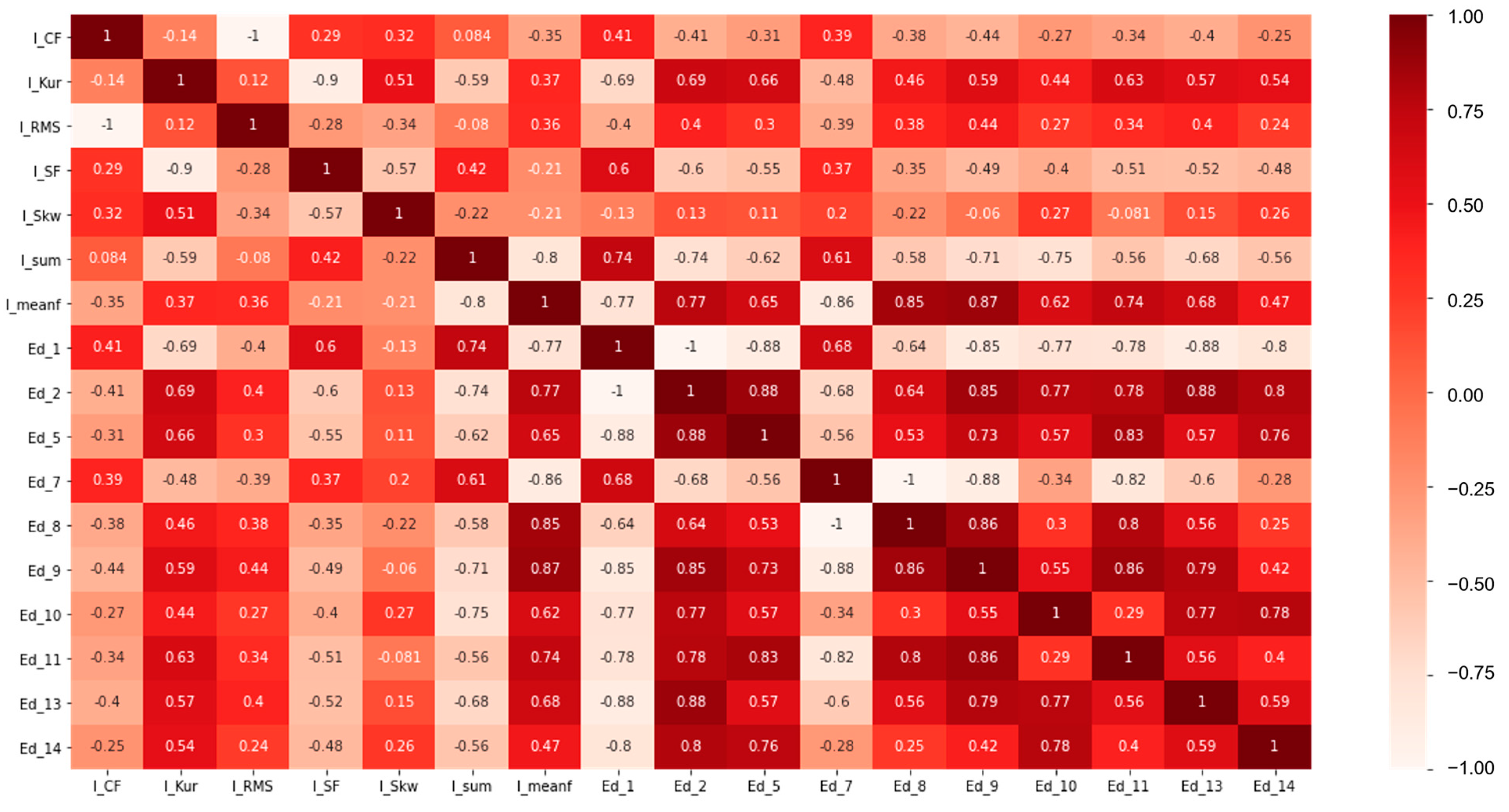Figure 12 is a heat map based on the Pearson correlation coefficient matrix of all of the data. The higher the correlation between each feature, the deeper the red color, and the more deeply the variables are related. By selecting only one of the features with a correlation coefficient of 0.9 or more, the number of features was reduced to 17, as shown in Figure 13. All of the features and 17 selected features are shown in

Table 3. All extracted features and features.

No	Parameters	Description/Values
1	$I_{CF}$	$I_{CF}$
2	$I_{CLF}$	$I_{Kur}$
3	$I_{IF}$	$I_{RMS}$
4	$I_{Kur}$	$I_{SF}$
5	$I_{RMS}$	$I_{skw}$
6	$I_{SF}$	$I_{sum}$
7	$I_{skw}$	$I_{meanf}$
8	$I_{STD}$	$E_1$
9	$I_{sum}$	$E_2$
10	$I_{var}$	$E_5$
11	$I_{meanf}$	$E_7$
12	$I_{medf}$	$E_8$
13	$I_{rmsf}$	$E_9$
14	$E_1$	$E_{10}$
15	$E_2$	$E_{11}$
16	$E_3$	$E_{13}$
17	$E_4$	$E_{14}$
18	$E_5$
19	$E_6$
20	$E_7$
21	$E_8$
22	$E_9$
23	$E_{10}$
24	$E_{11}$
25	$E_{12}$
26	$E_{13}$
27	$E_{14}$

. After feature selection, ANN is trained for Case V, and SVM is used for Case VI.

Figure 14 shows overall results of the proposed work related to fault classification. To elaborate further, Case I and Case II are based on the ANN and SVM classifiers, respectively, where all 27 features are used with random split for fault classification. Herein, 10-fold cross validation is used to overcome the overfitting issue. It is observed that the ANN-based fault classification shows a 92.15% training and 88.97% testing accuracy. On the other hand, the SVM-based classifier yields 91.5% and 92.97% of training and testing accuracy, respectively. The two proposed approaches show good classification performance, however, the number of features is higher, and it is computationally complicated to extract too many features. Besides, the ML classifier usually shows good performance with a large amount of data, and overfitting can be caused. In order to overcome these issues, the feature space is reduced using PCA and correlation analysis. In light of this, Case III and Case IV are based on the reduced feature space using PCA, and seven features are used. In Case III, the ANN classifier is used, achieving an 83.57% training and 81.45% testing accuracy. The SVM classifier is used in Case IV with a 90.01% and 90.67% training and testing accuracy, respectively. It is observed that the proposed feature selection method based on PCA shows good performance for fault classification. However, it is impossible to identify the exact type of feature in the process of feature reduction using PCA. For that reason, the feature space is reduced using the correlation analysis, as presented in Case V and Case VI, where 17 features are selected out of the original 27. In Case V, the ANN classifier is applied with an 87.05% training and 84.36% testing accuracy. On the other hand, the SVM classifier (Case VI) shows an effective performance with a 90% training accuracy and 91.76% testing accuracy. Overall, Case VI shows good performance in terms of the number of features and the classification performance. In conclusion, no significant difference was observed in the classification accuracy; however, the proposed approach overcomes the issues related to overfitting and computational complexities.

Table 4. Precision, sensitivity, F-1 score, and accuracy evaluation for the various presented cases.

	Case I	Case II	Case III	Case IV	Case V	Case VI
Precision	94.01	94.26	85.79	93.77	88.03	94.01
Sensitivity	84.34	91.53	79.81	87.85	88.25	89.55
F-1 score Accuracy	89.92 88.97	92.87 92.97	82.69 81.45	90.71 90.67	88.14 84.36	91.73 91.76

summarizes the precision, sensitivity, and F-1 score for all six cases. Precision represents the proportion of actual normal data to the predicted normal data. The formula is as follow [36]:

$$\mathrm{Precision}=\frac{True Positive}{True Positive+False Positive}$$

(9)

Sensitivity (called recall) represents the ratio of predicted normal data to actual normal data. The formula is as follows [36]:

$$\mathrm{Sensitivity}=\frac{True Positive}{True Positive+False Negative}$$

(10)

F score is the weight harmonic average of precision and sensitivity, and the case where the weight is 1 is called the F-1 score. The formula is as follows [36]:

$$\mathrm{F}-1\mathrm{score}=2\frac{\mathrm{Precision}\times \mathrm{Sensitivity}}{\mathrm{Precision}+\mathrm{Sensitivity}}$$

(11)

These are the performance evaluation parameters that are generally used to evaluate the performance of the classifiers. In general, compared to other performance evaluation indicators, it shows good performance in precision at 94.01 (Case I), 94.26 (Case II), 85.79 (Case III), 93.77 (Case IV), 88.03 (Case V), 94.01 (Case VI) and weak sensitivity at 84.34 (Case I), 91.53 (Case II), 79.81 (Case III), 87.85 (Case IV), 88.25 (Case V), and 89.55 (Case VI). This indicates that the models have high reliability in predicting normal data, but low reliability in predicting actual normal data. In addition, the F-1 score is almost similar to the accuracy, indicating that there is no imbalance problem in the data and that the amount of normal data and failure data is balanced.

To sum up, the proposed study is a robust approach for the fault detection of the robotic serve-motor. Our team proposed MCSA for fault detection in the robotic system for the first time. Using this method, the issues related to data handling and the installation of extra sensors are resolved. In order to reduce the discrepancy of a lab-scale model with real-world applications and increase the robustness of the model, various experiments are performed under variable working conditions, such as motion, speed, and loading. In this study, a feature engineering framework is proposed for fault classification based on ML applications. In the proposed work, various issues are resolved regarding overfitting and computational complexities. In future consideration, deep learning and transfer learning approaches can be used to improve the generalization capabilities of the fault detection model. With this research, we developed a fault detection model that generally works under different operating conditions than previous works. However, even though the proposed model does a good job of classifying the robot’s different modes of operation, data preprocessing needs to be made easier for real-time fault detection.

5. Conclusions

This study presented a method for developing a robust fault detection model for the servo motor of a robotic arm under various operating conditions. A method was proposed to improve classification performance under various operating conditions of robot arm speed, load, and motions. Performance was evaluated by comparing feature reduction methods or feature selection methods following feature extraction. The normal and abnormal data of a 6-axis industrial vertical robot’s third-axis servo motor were collected. MCSA was used to detect the faulty features of the inner race-bearing fault of the servo motor.

The proposed model extracts a total of 27 features in the time domain, frequency domain, and time–frequency domain, and the generalization ability of the model is improved by extending the range of feature extraction. When a fault occurred, the fault features were detected in various features of each cycle, and it was confirmed that the features were distinguished, especially in the high-frequency region. Cases in which features were reduced by PCA analysis were divided into those where the number of features was selected by correlation analysis. The two machine learning algorithms were trained for each case. Through case studies, cases with the highest accuracy were selected based on their computational efficiency.

As a result of comparing the accuracy of the learned model with the data from each test, it was confirmed that the original data with all features showed the highest accuracy—92.97%—in Case I. However, in Case VI, it was confirmed that a good classification model of 91.76% accuracy could be obtained as a result of a feature selection method that is computationally economical with little sacrifice of accuracy. Therefore, the present study shows that failures can be detected with an accuracy of more than 90% for various operating conditions such as the speed, load, and motions of the robot.

Conclusively, the main contributions are:

• This method works for various operating speeds, loads, and motions of the robot with acceleration and deceleration.
• Using time-domain, frequency-domain, and time–frequency-domain features, the range of feature extraction is extended, and the generalization ability of models is improved.
• The computational speed and the amount of feature computation can be reduced by using feature reduction and feature selection methods.
• A classification accuracy of over 90% can be achieved under various robot operating conditions.

The robustness of the proposed method under various operating conditions was evaluated using datasets with various speeds, loads, and motions. The classification accuracy of the proposed approach is above 90%.