Article

Improved Hybrid Firefly Algorithm with Probability Attraction Model

1
College of Engineering, Northeast Agricultural University, Harbin 150030, China
2
Computer Department, Shijiazhuang Posts and Telecommunications Technical College, Shijiazhuang 050020, China
*
Author to whom correspondence should be addressed.
These authors contributed equally to this work.
Mathematics 2023, 11(2), 389; https://doi.org/10.3390/math11020389
Submission received: 9 December 2022 / Revised: 5 January 2023 / Accepted: 9 January 2023 / Published: 11 January 2023

Abstract

:
An improved hybrid firefly algorithm with probability attraction model (IHFAPA) is proposed to solve the problems of low computational efficiency and low computational accuracy in solving complex optimization problems. First, the method of square-root sequence was used to generate the initial population, so that the initial population had better population diversity. Second, an adaptive probabilistic attraction model is proposed to attract fireflies according to the brightness level of fireflies, which can minimize the brightness comparison times of the algorithm and moderate the attraction times of the algorithm. Thirdly, a new location update method is proposed, which not only overcomes the deficiency in that the relative attraction of two fireflies is close to 0 when the distance is long but also overcomes the deficiency that the relative attraction of two fireflies is close to infinity when the distance is small. In addition, a combinatorial variational operator based on selection probability is proposed to improve the exploration and exploitation ability of the firefly algorithm (FA). Later, a similarity removal operation is added to maintain the diversity of the population. Finally, experiments using CEC 2017 constrained optimization problems and four practical problems in engineering show that IHFAPA can effectively improve the quality of solutions.

1. Introduction

Optimization problems widely exist in various fields of life. Traditional solving methods, such as the Newton method, conjugate gradient method and simplex method, need to traverse the entire search space, resulting in a combination explosion of search, that is, the search cannot be completed in polynomial time. In view of the complexity, constraint, nonlinearity and modelling difficulties in practical engineering problems, the research on meta-heuristic algorithms is particularly important. A meta-heuristic algorithm has the following advantages in solving complex engineering problems: (1) simple principle, fewer parameters to be adjusted and easy to implement; (2) do not need the derivative information of objective function; (3) differentiability and convexity are not required; (4) widely used to solve problems difficult to define with mathematical models or complex optimization problems; (5) strong, robust, versatile and suitable for parallel processing. Compared with traditional optimization methods, the probability of successfully escaping from the local optimal region is higher when solving complex problems, such as multi-extremum optimization. Therefore, meta-heuristic algorithms have great advantages in solving complex optimization problems and have been widely used in many fields.
Meta-heuristic algorithm includes the evolutionary algorithm as a key component. Evolutionary algorithms are primarily used to identify the best answer to optimization problems through the use of selection, crossover, mutation and other processes. The most well-known evolutionary algorithms are the genetic algorithm (GA) [1] and the differential evolution algorithm (DE) [2]. Population intelligence algorithms, as another important part of metaheuristic algorithms, update the position of individuals by simulating the behavior of animals, such as foraging, hunting and finding mates, to find the optimal solution of the optimization problem. In the past few decades, people have proposed many intelligence optimization algorithms, such as particle swarm optimization (PSO) [3], firefly algorithm (FA) [4], artificial bee colony algorithm (ABC) [5] and other swarm intelligence optimization algorithms. In 2008, Yang et al. [6] were inspired by fireflies’ luminous characteristics to attract mates and avoid natural enemies at night and proposed an FA. FA has the advantages of simple principles, few parameters, easy implementation, high precision and fast convergence. Therefore, the firefly algorithm is implemented to solve various problems in different domains, such as neural networks [7,8,9], scheduling problems [10,11,12], image processing [9,13], wireless parameter optimization of sensor networks [14,15,16] and big data processing [17,18].
Numerous academics have worked tirelessly over the past ten years to boost the FA’s effectiveness, with some promising study findings. In the FA, the attraction model greatly impacts the computational TC, convergence speed and solution quality in the algorithm. The more times of attraction in the attraction model, the faster the convergence speed of the algorithm and the worse the diversity of the population. The higher the TC, the easier it is to fall into a local optimum. In addition, the comparison times of fitness are different for different attraction models. The more fitness comparisons, the higher the time complexity (TC) in the algorithm. The attraction model used by the standard firefly algorithm (SFA) [6] is a complete attraction model (CAM). SFA can have an excess of attraction because each firefly can be attracted to another, with brighter fireflies in the population. Too much attraction can lead to oscillations or fluctuations in the algorithm search process, resulting in a poor quality algorithm solution. In 2016, Wang et al. proposed a firefly algorithm with random attraction (RaFA) [19]. RaFA uses a random attraction model (RAM) in which each firefly in the population is compared with another firefly chosen at random. If the brightness of the randomly selected firefly is higher than that of the current firefly, the current firefly is attracted by the randomly selected firefly; otherwise, the current firefly is not attracted. The RAM reduces the TC of the algorithm due to its smaller number of attractions, but also slows down the algorithm’s convergence due to the smaller number of attractions. In 2017, Wang et al. proposed a neighborhood attraction firefly algorithm (NaFA) [4], which uses a neighborhood attraction model (NAM), where brighter fireflies in the k-neighborhood are attracted to the current firefly. Although the NAM has a relatively moderate number of attractions, which has a greater possibility of reducing the premature convergence phenomenon, too many comparisons of too much brightness will lead to too much TC in the algorithm. In 2021, Cheng et al. proposed the hybrid firefly algorithm for group attraction (GAHFA) [20], which uses the grouping attraction model (GAM). GAHFA population size was even n, and all fireflies in the population were sorted and grouped according to the OFV, consisting of n/2 groups. Fireflies with high brightness in each group attract fireflies with low brightness, and fireflies with the highest brightness in the population attract fireflies with high brightness in each group. Although GAHFA has moderate attraction times and low TC in the algorithm, the attraction relationship between fireflies in the GAM is fixed, and it is easy to become stuck in a local optimum. To solve this problem, a new firefly attraction model, probabilistic attraction model, is proposed.
Use the example of an optimization problem where the goal function is the minimum value to demonstrate the issue. First, all fireflies are sorted according to fitness value from small to large. After sorting, the first firefly is the brightest firefly and the best firefly. Second, the first firefly in the population moves randomly. Third, starting from the second firefly, calculate the selection probability of each firefly. According to the selection probability of fireflies, select a brighter firefly from the fireflies in front of the current firefly. Fireflies are attracted to the brighter fireflies selected and so on. The probability attraction model can decrease the quantity of attraction times and brightness comparisons while preventing a situation in which there are insufficient numbers of both. In addition, the fireflies selected by the probability attraction model are random, which will reduce the possibility of the algorithm being trapped in local optimum. At the same time, the brightness of the firefly chosen by the probability attraction model is higher, which overcomes the drawback that the firefly chosen by the RAM cannot attract the present firefly.
The position-updating formula of the FA in the existing literature may have a phenomenon that the relative attractiveness tends to zero at the beginning of the iteration. The method conducts a random search because the relative attractiveness is 0, which causes a slow convergence of the algorithm and poor solution quality. In response to this problem, a formula for updating the position of the firefly with adaptive changes in relative attractiveness is presented. The relative attractiveness of adaptive changes will not approach zero in the iterative process. In addition, the location update formula not only considers the influence of high-brightness fireflies on the location-update fireflies but also considers the guiding effect of the best firefly in the population on the position-update fireflies.
In the later iteration of the algorithm, fireflies will gradually gather near the best fireflies, so the fitness difference among fireflies will be very small. In light of this circumstance, a formula is suggested to calculate the degree of similarity S among population members. The higher the similarity, the worse the diversity in the population and the lower the exploration ability of the algorithm; there is a high probability of getting trapped by a local optimum. The updating strategy of some individuals in the population is proposed to eliminate the similarity between individuals in the population. The update strategy is that, when S is less than the threshold, update some individuals in the population.
A combined mutation based on selection probability is proposed to dynamically select a single mutation operator with strong exploration and exploitation ability. This will further improve the solution quality and convergence speed of the algorithm and better balance the FA’s exploration and exploitation ability. In the early stages of the algorithm’s iteration, the combined mutation operator based on selection probability has a large chance of selecting a single mutation operator with strong global ability; in the later phases of the iteration, the probability of selecting a single mutation operator with strong local ability is high. First, according to the exploration and exploitation ability of each single mutation operator, multiple mutation operators are divided into two categories. The single mutation operator in the first category has a strong exploration ability, and the single mutation operator in the second category has a strong exploitation ability. Second, a formula is designed to calculate the selection probabilities of the two types of mutation operators based on improvements in the solutions to the optimization problems of the two types of mutation operators. A type of mutation operator has a bigger selection probability if it can enhance the quality of the problem’s solution, whereas if it cannot, it has a reduced selection probability. Each mutation operator within each category is chosen at random.
The major contributions of this paper are:
  • According to the uniformity and diversity of the initial population generated by different initialization methods, the best method of population uniformity and diversity is selected as the population initialization method.
  • A probabilistic attraction model is proposed for the problems of various attraction models.
  • A firefly position update formula with an adaptive change in relative attraction is proposed to improve the convergence speed and solution quality of FA.
  • A combined mutation operator based on selection probability is proposed, which can adaptively select a single mutation operator with strong exploration ability and exploitation ability.
  • A remove similarity operation is added to the algorithm to enhance the exploration ability of the algorithm and maintain the diversity of the population.
  • The proposed IHFAPA is compared with other improved algorithms in the literature in parameter optimization, such as reducer and cantilever beam. IHFAPA is superior to them in solution quality.
The organization of the rest of this paper is: Section 2 reviews the existing firefly algorithms; in Section 3, an IHFAPA is proposed; in Section 4, the proposed IHFAPA algorithm is experimentally analyzed using the CEC 2017 test function set and the performance is compared with other algorithms; Section 5 utilizes the IHFAPA algorithm to solve four classical engineering optimization problems, which is then compared with other algorithms; Section 6 is the Conclusion.

2. Related Works

2.1. Firefly Algorithm

In 2008, Yang proposed an FA based on the luminous characteristics of fireflies and the principle of mutual attraction between individual fireflies [6]. In order to construct the FA, some characteristics of the firefly flash need to be idealized. The specific idealization criteria are as follows:
(1) Fireflies are male and female, that is, fireflies are attracted to each other.
(2) Attraction is proportional to the brightness of fireflies. For any two fireflies, the high-brightness fireflies attract the low-brightness fireflies and move toward them, and the brightest fireflies move randomly.
(3) The brightness of fireflies is determined by the OFV of the problem to be optimized. Let n be the population size, the i-th firefly in the population is Xi = (xi1, xi2, …, xiD)T (i = 1, 2, …, n) and D is the dimension of the variable. The distance rij between any two fireflies i and firefly j in the population is:
r i j = | | X i X j | | = k = 1 D ( x i k x j k ) 2
where Xi and Xj are the i-th fireflies and j-th fireflies in the population, xik is the k component of the firefly i in the population and xjk is the k component in the j-th firefly in the population.
The attraction of firefly i to firefly j βij(rij) is:
β i j ( r i j ) = β 0 e γ r i j 2
where β0 is the maximum attraction, that is, when the attraction rij = 0, usually β0 = 1.
If the brightness of firefly j is higher than that of firefly i, firefly i is attracted by firefly j and moves toward firefly j. The location-update formula of firefly i is:
x i k ( t + 1 ) = x i k ( t ) + β i j ( x j k ( t ) x i k ( t ) ) + s t e p ( r 0.5 )
where t is the number of iterations; step is the step factor step ∈ [0,1]; r is a random number between [0,1].
The pseudo code of the standard firefly algorithm is shown in Algorithm 1.
Algorithm 1: Pseudo code of FA
Input: The population size of the population is n, and the dimension of the variable is D, T is maximum number of iterations;
Output: The final population;
Randomly generate n initial fireflies;
Calculate the fitness value of all initial fireflies;
Parameter initialization, population size, maximum attraction and light attraction coefficient; let t = 0;
  While t ≤ T do
     tt + 1;
      for i = 1 to n do
       for j = 1 to n do
         If firefly j is brighter than firefly i then
           Generate a new firefly according to Equation (3);
           Evaluate the new solution;
          End if
        End for
      End for
      Rank the fireflies and find the current best;
  End While
End

2.2. Brief Review of FA

FA has received wide attention from many scholars because of its simple concept, fewer parameter settings and easy implementation. In the past decade, the research results on FA improvement have mainly focused on the adaptive adjustment of parameters, the improvement in position update formula, the improvement in attraction model and the hybrid firefly algorithm.

2.2.1. Adaptive Adjustment of Parameters

The performance of the FA is significantly influenced by the parameters in the position-update formula, and the adaptive adjustment parameters can significantly enhance the algorithm’s performance. As a result, numerous researchers have examined parameter adaptive adjustments in the algorithm and proposed numerous adjustment methods. In 2012, Leandro et al. [21] proposed the light-absorption factor γ and step factor α adaptive adjustment firefly algorithm (CFA). CFA introduces Tinkerbell map in the light-absorption factor γ, which reduces the probability of the FA falling into a local optimum. The step size factor α in the CFA algorithm decreases linearly with the number of iterations, which better balances the exploration and exploitation ability of the algorithm. In 2013, Rizk-Allah et al. [22] proposed a method of non-linearly adjusting the step-size factor. The step-size factor decreases non-linearly with the increase in the number of iterations, which avoids disturbances in the optimal position of the firefly by the random term. Liang et al. [23] proposed an enhanced FA, which achieves a balance between exploration and exploitation ability by dynamically adjusting the step factor α. In the initial stage of the iteration, the value of α is large and the algorithm’s exploration ability is strong; in the later stage of the iteration, the value of α is small and the algorithm’s exploitation ability is strong. In 2017, Wang et al. [4] proved that when the number of iterations approached infinity and the limit of the step factor α was equal to 0, the algorithm converged, and they proposed a new method for dynamically adjusting the step factor α. The step factor α in this method decreases rapidly with the increase in iteration times and finally approaches zero, thus, ensuring the convergence of FA. In 2018, Banerjee et al. [24] proposed a firefly algorithm (PropFA) based on a new parameter-adjustment mechanism. In this mechanism, all parameters in the FA are dynamically adjusted according to the value of the objective function, striking a balance between exploration and exploitation. Experiments show that Prop FA performs better than other comparison algorithms. In 2019, Zhang et al. [25] proposed a dynamic adjustment in step-size factor α to improve the firefly algorithm. The results show that this method has better performance than other algorithms. In 2020, Amit et al. [26] proposed an improved firefly algorithm that considers the initial brightness β0 of environmental factors. The initial brightness of the algorithm changes dynamically, thereby achieving a better balance between exploration and exploitation. However, the algorithm does not consider the situation where the attractiveness value β is 0 when the two fireflies attracting each other in the population are far apart, which affects the performance of the algorithm.

2.2.2. Improved Location-Update Method

Location update is a crucial component in the FA and has a significant impact on how well the algorithm can optimize. The convergence speed and solution accuracy of the algorithm can be increased by optimizing the FA’s location-updating procedure. In 2016, Wang [19] and others proposed an improved firefly algorithm that replaces full attraction with random attraction, which greatly reduces the number of attractions and reduces the TC in the algorithm. However, the RAM may cause slow convergence of the algorithm and poor solution quality due to too few attraction times. In 2018, Zhan et al. [27] proposed an improved firefly algorithm, which introduced accelerated attractiveness and evading strategies into the location-update formula of the firefly algorithm. Accelerated attractiveness makes the current firefly converge in the vicinity of the optimal firefly faster, and the evading strategy keeps the current firefly away from the low-brightness firefly. The two operations can improve the convergence speed of the algorithm and reduce the probability of the algorithm falling into local optimum. In 2019, Wang et al. [28] proposed a firefly algorithm based on gender differences and designed two position-update formulas for fireflies of different genders. Male fireflies are attracted to two randomly selected females for global search; the female fireflies move to the vicinity of the best male fireflies for local search, which better balances the exploration and exploitation ability of the algorithm. The problem with the gravity calculation formula of this algorithm is that when the two fireflies are far apart, the value of relative attraction approaches 0, which causes the algorithm’s update formula to not work. In 2020, Wu et al. [29] proposed an adaptive logarithmic spiral-Levy FA (ADIFA). ADIFA designed two position-update formulas: the first position update formula Introduced Levy flight, which improves the exploration ability of the algorithm; the second position-update formula introduces the logarithmic spiral path, which improves the exploitation capabilities of the algorithm. In addition, an adaptive switch is also designed to realize the algorithm’s adaptive switching between exploration and exploitation modes. Experimental results show that the ADIFA algorithm is much better than the other three firefly algorithms.

2.2.3. Improvement in Attraction Model

The attraction model is an important part of the FA, which has a great impact on its performance. In 2008, the standard FA proposed by Yang et al. [4] used the CAM, in which each iteration can attract any brighter firefly in the population. In 2016, Wang et al. [19] proposed a random-attracting firefly algorithm to solve the problem that the algorithm too easily falls into local optimum due to too many times of attraction in the CAM. In each iteration of the random-attraction firefly algorithm, the i-th firefly in the population (i = 1, 2, …, n, n is the population size) matches the randomly selected j-th (j = 1, 2, …, n, i ≠ j) and compares the brightness of only fireflies. If the brightness of the j randomly selected firefly is higher than that of firefly i, firefly i will be attracted by firefly j. Otherwise, the i-th firefly will not be attracted by the j-th firefly. Compared with the CAM, the attraction times of the RAM are greatly reduced. Too few attraction times will cause the algorithm to converge slowly. In 2017, Wang et al. [30] proposed a firefly algorithm with neighborhood attraction. Each firefly in the population can be attracted by a brighter firefly in its k-neighborhood. The number of attractions in the NAM is relatively moderate, which can improve the convergence speed of the algorithm. Too much brightness comparison leads to high TC in the algorithm. In 2021, Cheng et al. [20] proposed a GAM. The GAM sorted the fireflies in the population according to the fitness value from small to large, and then the fireflies in the population are divided into n/2 groups. The fireflies with high brightness in each group attract the fireflies with low brightness. In addition, the best fireflies in the population also attracted bright fireflies in each group. Although the number of attraction times and the number of brightness comparisons are moderate in the GAM, since each firefly in the population is attracted by a fixed firefly, the algorithm easily falls into a local optimum.

2.2.4. Hybrid Firefly Algorithm

A single intelligence optimization method is constrained by the program’s structure or conditions that are associated with it and it easily falls into local optimum, producing subpar solutions. In order to fully exploit various intelligence optimization algorithms, the hybrid optimization algorithm combines two or more intelligence optimization algorithms or optimization ideas. Furthermore, the advantages of optimization ideas can improve the algorithm’s performance. In 2013, Huang et al. [31] proposed a hybrid firefly algorithm combining local random search methods, which effectively improved the local search ability of the algorithm (HFA). In addition, HFA is applied to reduce the jacket loss of downhole transmission and good results are achieved. In 2016, Verma et al. [32] proposed a hybrid firefly algorithm based on reverse learning (ODFA). ODFA uses reverse learning to optimize the position of the initial solution and improve the quality of the initial population. In 2017, Dash et al. [33] proposed a hybrid meta-heuristic algorithm that mixes the firefly algorithm and the differential evolution algorithm. The algorithm takes full advantage of the strengths of the firefly algorithm and the differential evolution algorithm and is well balanced, with improved algorithm exploration and exploitation ability. In 2018, Aydilek et al. [34] proposed a hybrid algorithm combining the firefly algorithm and particle swarm algorithm (HFPSO). The algorithm makes use of the fast convergence of PSO for global search and the fine tuning of FA for the local search, to balance the relationship between algorithm exploration and exploitation. The experimental results of the two test function sets, CEC 2015 and CEC 2017, show that HFPSO is significantly better than other algorithms. In 2019, Li et al. [35] proposed a hybrid firefly algorithm that embeds the cross-entropy method into the firefly algorithm. The method uses adaptive smoothing and co-evolution to fully absorb the robustness, ergodicity and adaptability of the cross-entropy method. This hybrid algorithm enhances the global search ability of the algorithm, stops the algorithm from falling into local optimization and improves the convergence speed of the algorithm. In 2020, Wang et al. [36] proposed a hybrid firefly algorithm that introduces a learning strategy containing Cauchy mutation into the firefly algorithm. In each iteration, the best firefly must implement L learning strategies to better balance the relationship between exploration and exploitation. However, the value of L is too large, which greatly increases the TC in the algorithm and will cause the algorithm to fall into a local optimum.

3. Proposed Methods

3.1. Population Initialization

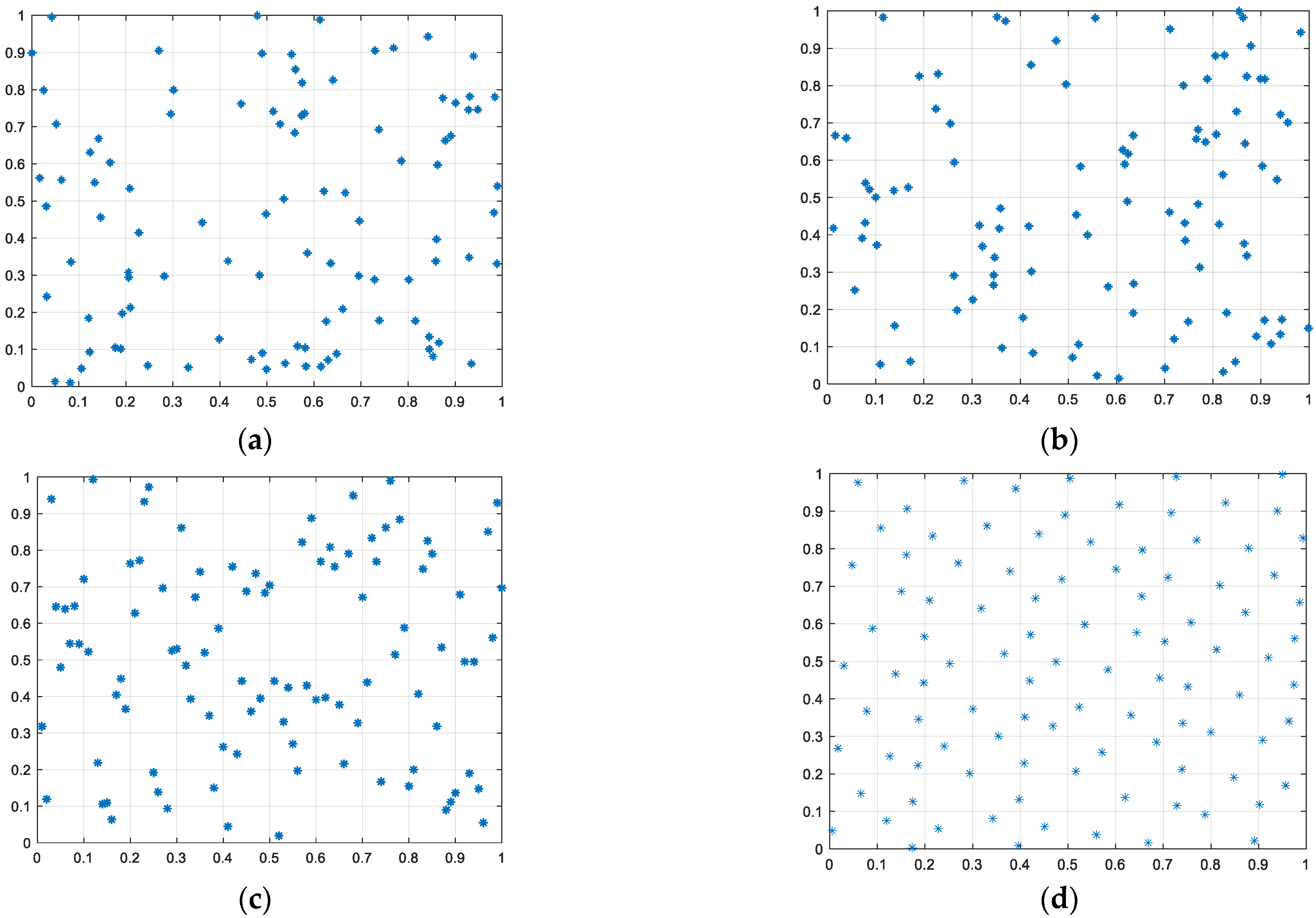
3.1.1. Initial Population Generation Method Based on Square-Root Sequence Method

The good point set theory was first proposed by Hua Luogeng and Wang Yuan in the book “The Application of Number Theory in Approximate Analysis” [37]. The point set generated based on this theory is evenly distributed in the unit space. Therefore, using the good point set theory can produce a uniformly distributed initial population in the search space, which can ensure the diversity of the initial population and reduce the possibility of the algorithm falling into local optimum. The specific steps of the initial population generation method based on the square-root sequence method are as follows:
Step 1: use the square-root sequence method to generate the first good point in the unit cube, that is, r1 = ( r 1 1 , r 1 2 , …, r 1 D ), where, r 1 j = { p j }, j = 1, 2, …, D. p1, p2, …, pD is D prime numbers from small to large; {•} represents the decimal part.
Step 2: based on r1, generate a good point set containing n good points according to Equation (4) Pn = (r1,r2,…, rn).
r i j = { p j × i } ,   i = 1 , 2 , , n ; j = 1 , 2 , , D
where n is the population size and pj is the j-th prime among D prime numbers that are not equal from small to large. D is the dimension of the problem and {•} is the decimal part.
Step 3: map the good point set generated by the square-root sequence method to the search space to obtain the initial population X of the population. The method of mapping the good point set to the search space is:
X i = L b + ( U b L b ) r i
where Xi is the i-th individual in the population, Ub and Lb are the upper and lower bounds of the search space, ri is the i-th good point in the good point set Pn and ⊗ is the product of the corresponding elements of the two vectors.
The method of initial population generation is shown in Algorithm 2.
Algorithm 2: Initial population generated based on the square-root sequence good point set method
Input: The population size of the population is n, and the dimension of the variable is D;
Output: The initial population of the population;
Produce the first good point r1:
Generate a good point set according to Equation (4) Pn
for I = 1 to n do
  The individual generating the initial population according to Equation (5) Xi:
end for

3.1.2. Compare Different Population Initialization Methods

The commonly used population initialization methods include random initialization method, population initialization method based on chaotic mapping, population initialization method based on reverse learning and population initialization method based on good point set theory. The random initialization method is simple in principle and easy to implement. Many references [19,38] use this method to generate the initial population and achieve good results. Chaotic mapping has the characteristics of randomness, ergodicity and regularity. Many scholars often use chaotic mapping to generate an initial population. In 2005, Yu et al. [39] took the lead in using chaotic mapping to generate an initialization population in GA, which effectively improved the optimization accuracy of the algorithm. Since then, many scholars have used chaotic mapping to generate initialization populations [40,41,42]. There are more than ten kinds of chaotic mappings. The chaotic mappings commonly used to generate the initial population are logistic mapping and tent mapping. The initial population generated by logistic mapping is mainly distributed at both ends of the search space, and the middle region less so. If the optimal solution is in the middle region of the search space, the convergence speed of the algorithm will be reduced. Tent mapping has better ergodicity and uniformity than logistic mapping, so tent mapping is often used to generate the initial population. In 2005, Tizzoosh et al. [41] proved that both the current solution and the elite individual have a 50% probability that they are far from the optimal solution compared to the reverse solution. In 2008, Rahnamayan et al. [40] used the population initialization method based on reverse learning to generate the initial population and achieved good results. Good point set theory is a point set generation method proposed by Professor Luogeng Hua [37]. It is mathematically proved that the point sets generated by good point set theory are evenly distributed in unit space. There are three major ways to generate point sets in the unit cube: exponential sequence method, circular domain method and square-root sequence method. Because the number of digits after the decimal point that can be displayed by the computer is limited, when the dimension is greater than 35, the decimal part of the number generated by the exponential sequence ek is 0, and the exponential sequence method is invalid. Therefore, the initial population can be generated using the split-circle domain method or the square-root sequence method.
The advantages and disadvantages of the initial population generated by different methods can be judged according to the uniformity of individual distribution in the search space and the polyphase of the population. In order to clearly describe the uniformity of the initial population generated by different methods in the search space, taking a population size of 100 and a variable dimension of 2 as examples, the initial population is generated in the interval [0,1] by using the random initialization method, the population initialization method based on tent mapping, the population initialization method based on reverse learning and the population initialization method based on the square-root sequence method. The initial population generated by different initialization methods is shown in Figure 1.
From Figure 1, the initial population generated by the random initialization method, the population initialization method based on tent mapping and the population initialization method based on reverse learning have the phenomenon of uneven distribution and aggregation. If the optimal solution is far away from the aggregation region, the convergence speed of the algorithm will be slow and it easily falls into a local optimum. The initial population generated by the population initialization method based on square-root sequence is dispersed in the whole search space and there is no aggregation phenomenon. Therefore, the initial population is generated based on square-root sequence.
The variety in the population has a significant effect on how well the algorithm performs. Good population variety makes it difficult for the algorithm to fall into premature convergence. A population diversity computation method is provided in order to quantitatively compare the diversity in the starting population created by various population initiation methods. The calculation method of population diversity is:
D i v e r s i t y = 2 n ( n 1 ) i = 1 n 1 j = i + 1 n d ( X i , X j )
where n is the population size, Xi is the i-th firefly, Xj is j-th firefly in the population and d (Xi, Xj) represents the Euclidean distance between the i-th firefly and the j-th firefly. The calculation formula of d (Xi, Xj) is as follows:
d ( X i , X j ) = k = 1 D ( x i k x j k ) 2
where D is the dimension of the variable, xik is the k-th component of the i-th firefly and xjk is the k-th component of the j-th firefly.
In Equation (6), the value of Diversity is proportional to the distance between individual fireflies in the population. The greater the distance between individual fireflies, the greater the value of Diversity; the smaller the distance between individual fireflies, the smaller the value of Diversity. The greater the value of Diversity, the more uniform the distribution of individuals in the population, and the less likely it is the algorithm will fall into local optimum; the smaller the value of Diversity, the more likely it is that there is individual clustering in the population, and the easier it is for the algorithm to fall into local optimum.
According to Equation (4), the diversity in the initial population generated by the above four methods is calculated, and the calculation results are given in Table 1.
In Table 1, the population initialization method based on the square-root sequence method produces the best initial population diversity, followed by the population initialization method based on tent mapping and the population initialization method based on reverse learning, then for the initial population generated by the random initialization method, the population diversity in the population is the worst.
In conclusion, whether it is population diversity or population uniformity in the search space, the initial population produced by the population initialization approach based on the square-root sequence method is the best. Therefore, the square-root-sequence-based population initialization approach is chosen as the population initialization method.

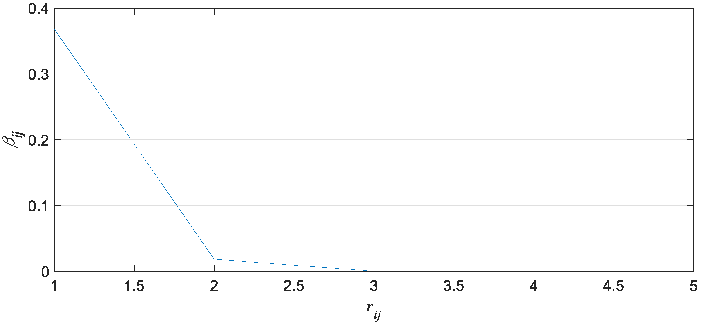
3.2. Probability Attraction Model

3.2.1. Common Attraction Model

In the existing literature, the commonly used attraction models are: complete attraction model (CAM), random attraction model (RAM), neighborhood attraction model (NAM) and grouping attraction model (GAM). In order to facilitate the statistics of the attraction times and brightness comparison times of various attraction models, let the population size of FA be n and the objective function is the minimum.
In the CAM, each firefly is attracted by other brighter fireflies in the population at each iteration. The individuals in the population are sorted according to the OFV from small to large. Since each firefly will only be attracted to other brighter fireflies, the first firefly (the best firefly) is not attracted and the number of attractors is 0; the second firefly is only attracted by the first firefly, and the number of attractions is 1. By analogy, the last firefly (the worst firefly) in the population will be attracted by all other fireflies, and the number of attractions is n − 1. Therefore, the total attraction times T1 of the CAM are:
T 1 = 0 + 1 + 2 + + n 1 = n ( n 1 ) 2
According to Equation (8), the total attraction times T1 of the CAM T1 = n (n − 1)/2, then the average number of attractions t1 = T1/n = (n − 1)/2 for each firefly.
For the FA using the CAM, each firefly must judge whether it is attracted by other fireflies. Therefore, the n fireflies in the population need brightness comparison. When comparing brightness, each firefly needs to compare brightness with another n − 1 firefly, then the total brightness comparison times of n fireflies are T2 = n (n − 1), and the average brightness comparison times of each firefly are t2 = n − 1.
In the NAM [30], each firefly is attracted by a brighter firefly in the k-neighborhood during iteration. The k-neighborhood of Xi consists of 2k + 1 fireflies {Xi-k, …, Xi, …, Xi+k}, where k is an integer and 1 ≤ k ≤ (n − 1)/2. k in reference [42] is much smaller than (n − 1)/2. In order to analyze the times of attraction in each iteration, firstly, the fireflies are sorted according to the OFV from small to large. After sorting, the first firefly is the firefly with the highest brightness and the nth firefly is the firefly with the darkest brightness. Secondly, all fireflies are linked to a ring topology according to the indicator order 1, 2, …, n. The total attraction times of all fireflies are T1 = 0 + 1 + … + k − 1 + k + k + 1 + k + 2 + … + 2k − 1 + 2k = kn, and the average attraction times of each firefly are t1 = T1/n = k. Each firefly needs to compare its brightness with all other fireflies in its k-neighborhood. The total brightness comparison times are T2 = 2kn, and the brightness comparison times of each firefly are t2 = 2k.
In the RAM [19], each firefly compares its brightness with another randomly selected firefly in each iteration. Only the fireflies move; otherwise, they do not move. Therefore, the maximum number of attraction times for all fireflies is T1 = n, and the average number of attraction times for each firefly is t1 = 1. Since each firefly has to be compared with another randomly selected firefly, the number of times of brightness comparison for each firefly is 1. For the RAM with a population size of n, the total number of comparisons of the brightness of all fireflies is n, and the number of comparisons of the average brightness of each firefly is t2 = 1.
In the GAM [20], there are two fireflies in each group. In each iteration, the fireflies with low brightness in each group are attracted by the fireflies with high brightness, and the fireflies with high brightness in each group are also attracted by the fireflies with the highest brightness in the population. Therefore, the total attraction times of all fireflies are T1 = n − 1, and the average attraction times of each firefly are t1 = T1/n = (n − 1)/n. In the GAM, the brightness of two fireflies in each group should be compared. There are n/2 groups, which need to be compared n/2 times; the firefly with high brightness in each group needs to be compared with the highest firefly in the population for (n − 1)/2 times. Therefore, the sorting of n fireflies requires n − 1 comparisons, and the average brightness comparison times of each firefly t2 = (n − 1)/n.
The population variety is worse, the TC is higher and local optimization is simpler to fall into as there are more times of attraction. Additionally, for different attraction models, there are various brightness comparison times. The algorithm’s TC increases with the number of fitness comparisons. For a good attraction model, the attraction times and brightness comparison times should be moderate, and the selection of fireflies with high brightness should be adaptive or have a better guiding effect on the attracted fireflies. A new attraction model known as the probability attraction model is developed in order to make the attraction times and brightness comparison times of the attraction model modest and to make the attraction model adaptive while choosing fireflies with high brightness.

3.2.2. Probability Attraction Model

To facilitate the description of the probability attraction model, suppose the population size is n and the objective function of the optimization problem is to find the minimum. If the objective function is to seek the maximum value, the objective function can be changed to seek the minimum value according to max P(X,M) = −min[−P(X,M)]. In addition, in order to make the probability attraction model adaptive in choosing to attract fireflies, and to make the attracted fireflies have a better guiding effect on the attracted fireflies, all the fireflies in the population are sorted according to their OFV and the selection probability of each firefly is calculated. When selecting to attract fireflies, the fireflies with a high probability of selection have a high probability of being selected as attracting fireflies. In the GAM, a firefly is used to attract fireflies, and a firefly in the probability attraction model is selected, as attracting fireflies is determined by its selection probability. The firefly with high probability of selection has a greater probability of being selected as an attractive firefly. Therefore, the probability attraction model is adaptive in choosing to attract fireflies. At the same time, the selected attracting fireflies have a better guiding effect on the attracted fireflies. The specific steps in the probability attraction model are as follows:
(1) Order fireflies according to the OFV from small to large.
(2) Calculate the selection probability of each firefly after sorting. The calculation formula for selection probability is:
P k = f i t ( k ) j = 1 i 1 f i t ( j ) ( i = 2 , 3 , , n ; k = 1 , 2 , , i 1 )
f i t ( k ) = λ × ( 1 λ ) k 1 ( k = 1 , 2 , , n 1 )
where Pk is the selection probability of the k-th individual in the population, λ is a constant between 0.01 and 0.3, and λ = 0.15, fit(k) is the fitness value of the k-th firefly.
(3) According to the selection probability Pk (k = 1,2, …, n − 1) of each firefly, calculate the cumulative probability PPk (k = 1,2, …, n − 1) of each firefly. PPk is calculated as follows:
P P k = j = 1 k P j ( k = 1 , 2 , , n 1 )
(4) Choose to attract fireflies for the n-th firefly in the population. The selection method is to generate a random number rr evenly distributed in the interval [0,1]. If rr satisfies PPk − 1rr ≤ PPk (k = 2, 3, …, n − 1), the k-th firefly is selected as the attracting firefly. Selecting and attracting fireflies for the n − 1 firefly also requires generating a random number rr, and if rr satisfies PPk – 1rrPPk (k = 2, 3, …, n − 1), select the k-th firefly as the attracting firefly. By analogy, the n − 3, n − 4, …, 2th fireflies are selected to attract fireflies, and the first firefly is the best. It is not attracted by any fireflies and only moves randomly.
In summary, when the population size is n, the total number of attraction times is T1 = n − 1 and the average number of attraction times for each firefly is t1 = (n − 1)/n. The total number of brightness comparisons T2 = n(n − 1)/2, the average number of brightness comparisons of each firefly t2 = (n − 1)/2. The number of attraction times and the number of brightness comparisons of the five attraction models are shown in Table 2.
In Table 2, the total attraction times of the probability attraction model are less than the CAM and the NAM, which are equal to the GAM. For the RAM, if the randomly selected n fireflies have high brightness, the total attraction times of the probability attraction model are less than that of the RAM; otherwise, the total attraction times of the probability attraction model are greater than or equal to the RAM. For the average attraction times, the comparison result of the average attraction times of each firefly is the same as that of the total attraction times. In addition, the brightness comparison times of the probability attraction model are equal to the GAM, but less than the CAM, RAM and NAM.
To sum up, for the five attraction models, the probability attraction model and GAM have moderate attraction times and the least brightness comparison times. In the GAM, the attraction relationship between fireflies is fixed, that is, the attraction of the next n/2 fireflies to the first n/2 fireflies is unchanged, and the attraction from the second to the n/2 fireflies to the first firefly is also unchanged. In the probability attraction model, whether a firefly with low brightness is attracted by a firefly with high brightness is determined by the selection probability of the firefly with high brightness. When selecting to attract fireflies, it is adaptive and has a great probability to select the firefly with higher brightness, which has a better guiding role for the attracted firefly.
Therefore, the probability attraction model can avoid premature convergence caused by too many times of attraction and can also avoid too little attraction and reduce the convergence speed of the algorithm. When choosing to attract fireflies, according to the selection probability of fireflies, the selection strategy is adaptive and has a better guiding role for attracted fireflies. In addition, because the brightness comparison times of the probability attraction model are less, the TC in the algorithm can be reduced.

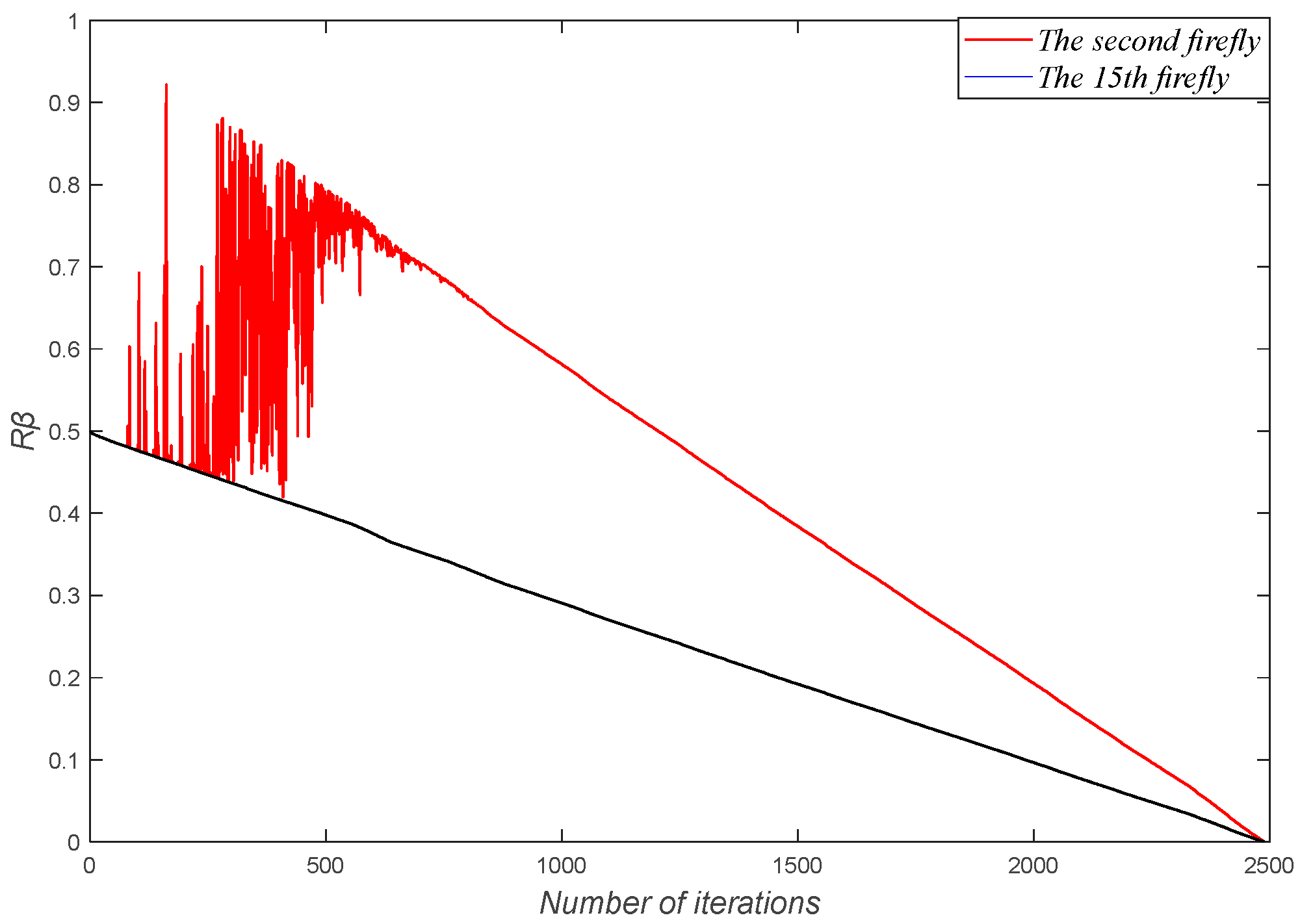
3.3. Improved Location-Update Method

In the firefly algorithm in the existing literature [6,43,44], the position-update formula and the calculation formula of relative attraction are:
x j ( t + 1 ) = x j ( t ) + β i j ( γ i j ) ( x i ( t ) x j ( t ) ) + α ε j
β i j ( r i j ) = β 0 e γ r i j 2
where the brightness of xi is higher than that of xj, βij is the relative attraction between firefly i and firefly j, β0 is the maximum attraction, γ is the light-absorption coefficient, rij is the distance between firefly i and firefly j, α is a constant and εj is a random number obtained from Gaussian distribution. For most problems, it can take β0 = 1, γ ∈ [0.01,100], α ∈ [0,1].
When γ = 1, the curve of relative attractiveness βij as the number of iterations increases is shown in Figure 2.
In Figure 2, the relatively attractive force βij decreases with the distance rij between firefly i and firefly j increases. When the distance between firefly i and firefly j is rij ≥ 3, the value of relative attraction βij(rij) approaches 0. At this point, the value of the attractive term βij in the position-update formula approaches 0, the βij has no effect, the position-update formula has no guiding effect and the algorithm degenerates into a random search with a slow convergence speed. At the same time, because of the relatively small value of the perturbation term αεj, the global search ability of the algorithm is weak, and it is easy to fall into local optimization. In addition, for a given problem to be optimized, if the value range of variables is large (for example, −100 ≤ xik ≤ 100, I = 1, 2, …, n, k = 1, 2, …, D), the distance between fireflies in the population after initialization is relatively far, and the value of relative attraction βij(rij) may approach 0, so the attraction term does not work. As the number of iterations increases, the distance between fireflies in the population decreases gradually and the value of relative attraction βij(rij) increases gradually. When rij < 3, the attraction term works, and with the increase in attraction βij(rij), the attraction term gradually increases, so the guiding effect of the firefly with high brightness in the position-update formula gradually increases and the convergence speed of the algorithm will be gradually improved. To solve the above problems, a new position-update formula is proposed. The new location-update formula is:
(1) Sort the fireflies according to their OFV from small to large.
(2) The fireflies in the population update their positions as follows.
{ X i ( t + 1 ) = X i ( t ) + β R ( X k ( t ) X i ( t ) ) + ( 1 R ) r a n d ( 1 , D ) ( X b e s t ( t ) X i ( t ) ) + α ( ε 0.5 ) X b e s t ( t + 1 ) = N ( X b e s t , | X b e s t X ¯ | 2 36 )
X ¯ = X 1 + X 2 + + X n n
where t is the number of iterations, Xi(t) is the position of the i-th firefly of generation t, Xi(t + 1) is the position of the i-th firefly in generation t + 1, Xbest(t) is the position of the best firefly in generation t, rand(1,D) is a random vector uniformly distributed between [0,1], Xk(t) is the position of the firefly selected by probability attraction in generation t, β is the position of the firefly i and the attraction between fireflies Xk, R is the adjustment coefficient, α is the dynamic step and ε is a uniformly distributed D-dimensional random vector between [0,1], ⊕ indicating that the elements of two vectors at the same position are multiplied.
βR(Xk(t) − Xi(t)) in Equation (14) is called the attraction term, (1 − R) rand (1, D) ⊕ (Xbest(t) − Xi(t)) is called the bootstrap term and α(ε − 1/2) is called the stochastic term. β and R are calculated as follows:
β = β min + ( β max β min ) e γ r i j 2
R = 1 r u n t i m e ( t ) M a x t i m e
where βmax is the maximum attraction, βmin is the minimum attraction (both are constants), γ is the light-absorption coefficient, usually taken as 1, runtime is the time of the current iteration and Maxtime is the maximum time for the algorithm to run.
From Equations (14) and (16), it can be seen that Equation (16) can avoid the attraction β being 0 at the beginning of the iteration, which leads to the phenomenon that the attraction term does not work. In addition, from Equation (16), at the beginning of the iteration, the fireflies are far away from each other, so the value of β is small, and with an increase in the number of iterations, the distance of fireflies gradually decreases, and the value of β gradually becomes larger; when the distance of fireflies is 0, the value of β reaches the maximum, at which time β = βmax. As the number of iterations increases, β becomes larger and R becomes smaller, so the trend of βR cannot be determined. To judge the changing trend of βR with the increase in the number of iterations, the C01 function in the CEC 2017 function set was chosen as the test function, and the βR values of the 2nd firefly and the 15th firefly at each iteration were kept, and a change curve of βR with an increase in the number of iterations was drawn, as shown in Figure 3.
Figure 3 illustrates that the value of βR decreases with an increase in the number of iterations. At the beginning of the iteration, the value of βR is larger, the distance between fireflies in the population is relatively far, the value of Xk(t) − Xi(t) is larger and the value of βR(Xk(t) − Xi(t)) is larger. In addition, it can be seen from Equation (17) that at the beginning of the iteration, the value of R is larger, the value of 1R is smaller, the value of rand(1, D)(1 − R) is even smaller and the value of rand(1,D)(1 − R)( Xbest(t) − Xi(t)) is also smaller. At the beginning of the iteration, the term βR(Xk(t) − Xi(t)) plays a major role, then the algorithm’s global search ability is strong; at the later part of the iteration, the distance between fireflies becomes smaller compared with the beginning of the iteration and the value of Xk(t) Xi(t) is also decreasing compared with the beginning of the iteration. In addition, in the later stage of the iteration, the value of βR gradually decreases. Hence, in the later stage of the iteration, the value of βR(Xk(t) − Xi(t)) gradually decreases compared with the initial stage of the iteration, and the βR(Xk(t) − Xi(t)) term has a weaker influence on the change in firefly position. As the value of R gradually becomes smaller in the later iterations, the value of 1 − R gradually becomes larger and the value of rand(1,D)(1 − R)(Xbest(t) − Xi(t)) gradually changes in a large manner. Therefore, at the later stage of the iteration, the local search capability of the algorithm is enhanced. The position-update formula of the population can better consider the global search ability and local search ability of the algorithm.
The main content of the firefly population position update is given in Algorithm 3.
Algorithm 3: Improved position update based on probability attraction model
Input: individual fireflies of the population;
Output: the updated firefly population;
Calculation of the OFV for fireflies in the current population;
The fireflies in the population are sorted according to their OFV from small to large;
Recording the best firefly Xbest and its OFV fbest;
for i = 2 to n do
  Update Xi(t) and Xbest according to Equation (14);
End for

3.4. Combined Mutation Operator Based on Selection Probability

FA’s exploration and exploitation abilities are determined by the firefly’s location-update formula. The firefly location-update formulation given in the existing literature has a strong exploration capability in the early iteration and a strong exploitation capability in the late iteration, which can balance the exploration and exploitation ability of the algorithm to some extent. For a multiple-optimization problem, even if the iteration termination condition is the maximum number of iterations or the maximum running time, it is impossible to judge when it is the early stage of the iteration and when it is the late stage of the iteration. Therefore, estimating the early and late iterations based on the quantity of iterations or running duration is incorrect. According to the maximum number of iterations and the maximum running duration, there are two issues with determining the issues in the early and late iterations: First, the algorithm performs local search when local search is required and global search when local search is required. In addition, the algorithm does not need global search in each iteration in the early stages of iteration, and sometimes it may need local search; in the late stage of iteration, local search is not required for each iteration. If it falls into local optimum, global search is required. The combination mutation operator in the literature [20] selects a single mutation operator according to the same probability. It is possible that when a mutation operator with strong exploration ability is needed, a mutation operator with strong exploitation ability is selected. A combined mutation operator based on selection probability is proposed to solve the above problem.
For the convenience of description, suppose the i-th firefly participating in the mutation operation is Xi(t) (i = 1, 2, …, n) and the firefly obtained after the mutation is Xi(t + 1) (i = 1, 2, …, n), b1, b2, b3, b4, b5 ∈ {1, 2, …, n}, and b1b2b3b4b5i, Xbest(t) is the best firefly in the t-th generation population. The four single variance operators selected are:
X i ( t + 1 ) = X b 1 ( t ) + F ( X b 2 ( t ) X b 3 ( t ) )
X i ( t + 1 ) = X b 1 ( t ) + F ( X b 2 ( t ) X b 3 ( t ) ) + F ( X b 4 ( t ) X b 5 ( t ) )
X i ( t + 1 ) = X b e s t ( t ) + F ( X b 1 ( t ) X b 2 ( t ) )
X i ( t + 1 ) = X b e s t ( t ) + F ( X b 1 ( t ) X b 2 ( t ) ) + F ( X b 3 ( t ) X b 4 ( t ) )
where F is the step size and the calculation formula of F is:
F = 0.4 + 0.6 × r
where r is a random number between [0,1].
The single mutation operators in Equation (18) to Equation (21) are divided into two categories: the first is the single mutation operator with strong exploration ability, including Equations (18) and (19); the second type is a single mutation operator with strong exploitation ability, including Equations (20) and (21). The calculation formula of the selection probability of the two types of mutation operators is:
P 1 = S 1 F 1 S 1 F 1 + S 2 F 2 = 1 1 + S 2 F 1 S 1 F 2
P 2 = 1 P 1
where P1 is the selection probability of the first type of mutation operator, S1 is the number of candidate solutions generated by the first type of mutation operator retained for the next generation, F1 is the number of candidate solutions generated by the first type of mutation operator that is not kept for the next generation, and S2 is the number of candidate solutions generated by the second type of mutation operator that is retained for the next generation and F2 is the number of candidate solutions generated by the second type of mutation operator that cannot be retained to the next generation. Generally, the initial values of S1, F1, S2 and F2 are taken as 1.
First, judge whether to choose the first type of mutation operator or the second type of mutation operator. The judgment method is randomly generating a random number μ between [0,1]. If μ < P 1, select the first type of mutation operator; if μP 1, select the second type of mutation operator. Secondly, judge whether to choose the first mutation operator or the second mutation operator in a certain class. The method of judgment is: randomly generate a random number λ between [0,1]; if λ < 0.5, select the first mutation operator in a certain type of mutation operator; otherwise, select the second mutation operator.
Algorithm 4 describes the main steps of combining mutation operators based on selection probability.
Algorithm 4: Combined mutation operation based on selection probability
Input: Firefly individuals in the population;
Output: Firefly individuals in the population after combined mutation operation;
Calculate the value of scaling factor f according to Equation (22);
for i = 1 to n
if rand < P1
if rand ≤ 0.5
Generate a new solution Xi(t + 1) according to Equation (18);
else
   Generate a new solution Xi(t + 1) according to Equation (19);
else
Else rand ≤ 0.5
   Generate a new solution Xi(t + 1) according to Equation (20);
  else
   Generate a new solution Xi(t + 1) according to Equation (21);
End if
End if
End for
Equations (23) and (24) report that, if a global search is required for the t-th iteration, if the second type of mutation operator is selected, the value of S2 is less than that of F2. Since the values of S1 and F1 remain unchanged, the value of (S2F1)/(S1F2) decreases and the value of P1 increases. The first type of mutation operator will probably be selected in the t + 1 iteration. If a global search is required for the t-th iteration, if the first type of mutation operator is selected, the value of S1 is greater than the value of F1. Since the values of S2 and F2 remain unchanged, the value of (S2F1)/(S1F2) decreases and the value of P1 increases. The first type of mutation operator will be selected with a high probability in the t + 1 iteration, and vice versa.
In conclusion, based on the historical contributions of the two types of mutation operators, the combined mutation operator based on the selection probability can choose which type of mutation operator is selected to perform the mutation operation in the following iteration. As a result, regardless of whether the algorithm is in an early or late iteration, the combined mutation operator based on the selection probability can flexibly select a particular type of mutation operator with high exploration or exploitation ability. In addition, due to the strong exploration ability of the first type of mutation operator, the contribution made at the beginning of the iteration is greater than that of the second type of mutation operator, so the first type of mutation operator is more likely to be selected, which improves the exploration of the algorithm ability. At the end of the iteration, the historical contribution of the second type of mutation operator is greater than that of the first type of mutation operator, so mutation operators of the second type are more likely to be selected, which improves the exploitation ability of the algorithm.

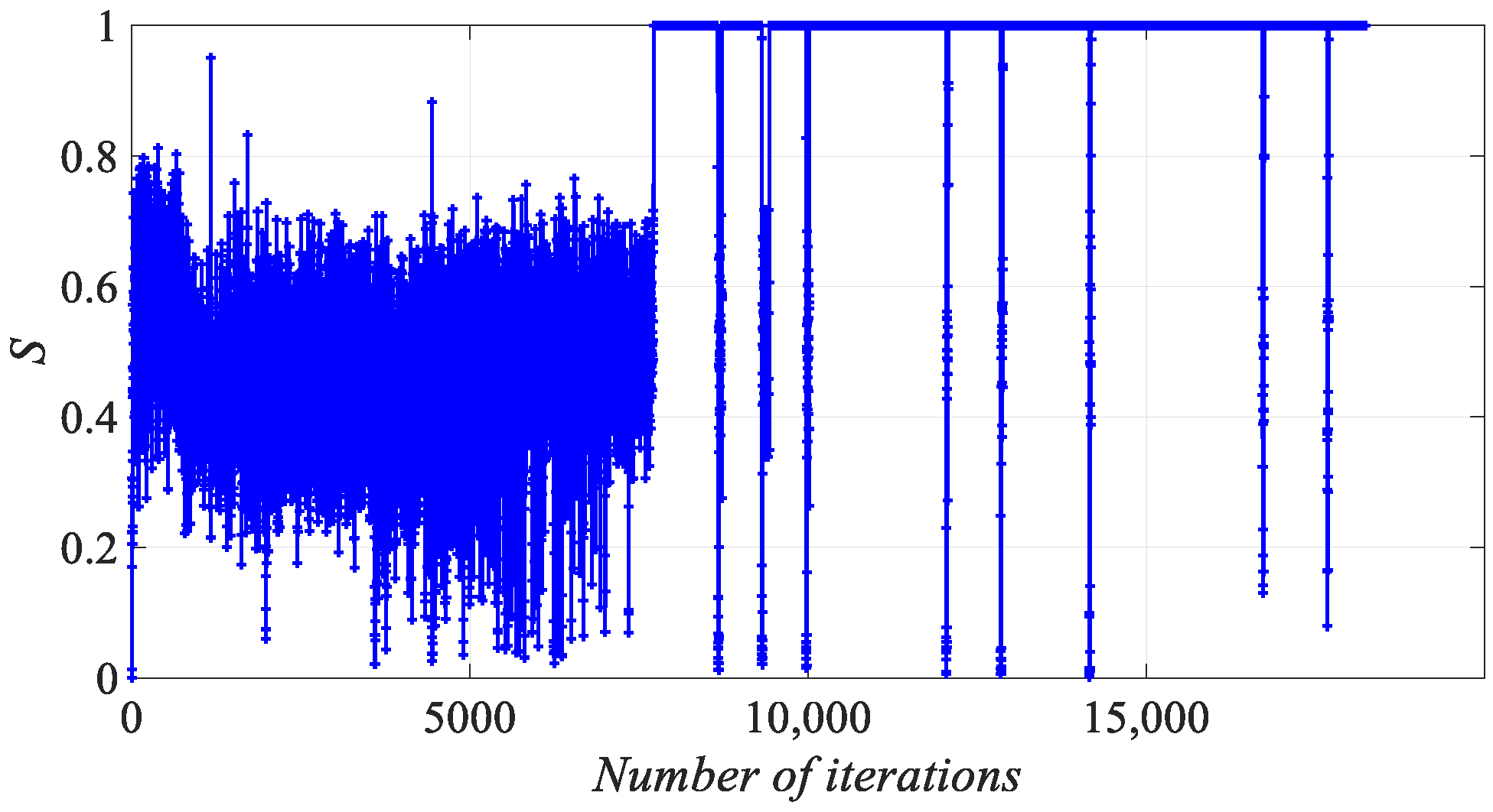
3.5. Remove Similarity Operation

Similar individuals mean that the difference in fitness values between individuals is less than a certain threshold ζ. There will be a large number of similar individuals in the population as iteration times rise. The population’s members are generally gathered close to the optimal firefly, especially later in the iteration. For the multi-extremum optimization problem, if the best individual in the population is near a local extremum, the algorithm can easily fall into a local optimum. Therefore, in the iterative process, similar individuals need to be removed from the population to maintain diversity. In order to keep the population size constant, similar individuals that were removed can be generated via the random initialization method. The specific steps in similarity removal are:
(1) Order the fireflies according to the OFV from small to large;
(2) Evaluate the similarity of fireflies. The formula for calculating the similarity S between fireflies in the population is:
S = f ( 0.5 n ) f ( 1 ) + e p s f ( n ) f ( 1 ) + e p s
where f(0.5n) is the OFV of the 0.5n firefly in the sorted population and f(1) is the OFV of the first firefly in the sorted population, f(n) is the OFV of the last firefly in the sorted population, eps is a small number, eps = 2.2204 × 10⁻¹⁶ and eps is used to avoid the denominator being zero.
(3) If S ≥ ζ, the similarity between fireflies in the population is higher and the population diversity is poor. In this case, the better q individuals in the population are retained, and the remaining n-q individuals are generated by a random initialization method.
To visualize the similarity degree of the population, the population is processed in two dimensions; let the population size be n = 40 and the number of dimensions of the variables be D = 2. In the iterative process of the algorithm, Figure 4 shows the degree of similarity in the population that does not use a remove-similarity operation, and Figure 5 illustrates the degree of similarity in the population after using a remove-similarity operation.
In Figure 4, the difference between the OFV of the first firefly and the last firefly is larger in the early iteration, and the difference between the OFV of the 0.5n-th firefly and the first firefly is also larger, so the S value is smaller. As the algorithm gradually iterates, the individuals in the population will slowly gather near the optimal individual, and the 0.5n firefly and the last firefly in the population also focus on the optimal individual. The difference between the OFV of f(0.5n) and f(n) gradually becomes smaller, and the value of S gradually increases. Due to the introduction of a combinatorial mutation operator in the algorithm, the S value is small occasionally, but it is not enough to jump out of the local optimum, so the value of S increases rapidly. From Figure 5, after adding the remove-similarity operation, the S value of the algorithm is small in most cases and large in occasional cases. When S ≥ ζ, the S value decreases rapidly, and the diversity in the population is better because of the increase in performing the remove-similarity operation in the population. Therefore, the addition of the remove-similarity operation increases the global search capability of the algorithm and reduces the probability of the algorithm falling into a local optimum.

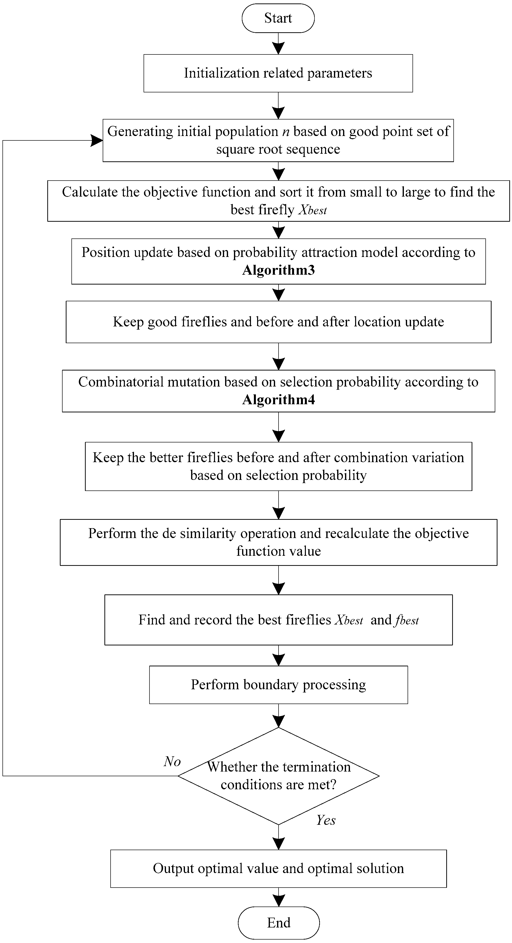
3.6. The Evolutionary Strategy of IHFAPA

The evolutionary strategy in the improved hybrid firefly algorithm with probability attraction (IHFAPA) is presented in Algorithm 5. Figure 6 shows a flow chart of IHFA-PA, which more clearly displays the specific steps in the algorithm. From Figure 6, we can see that the performance of IHFAPA is related to the location-update method, probability attraction model, combined mutation operator, remove-similarity operation and evolution strategy of fireflies. IHFAPA uses a new location-update method. Under the attraction of the high-brightness fireflies and the best fireflies, the low-brightness fireflies move to the high-brightness fireflies, which better balances the exploration and exploitation ability of the algorithm. Meanwhile, IHFAPA uses the combined mutation operator, which can be based on the historical contributions of the two types of mutation operators, to select a suitable single mutation operator to perform mutation operation adaptively according to needs. Combined mutation operators include two different single mutation operators, and each type of mutation operator has a different selection probability. If a certain type of operator has a greater contribution in the previous iteration process, then this type of operator has a greater probability of selection; on the contrary, this type of mutation operator has a smaller selection probability. In the iterative process, the selection probabilities of the two types of mutation operators are not static. As the historical contributions of the two types of mutation operators change, the selection probability will also change. Therefore, the combined mutation operator based on the selection probability can well balance the exploration and exploitation ability of the algorithm. In addition, a remove-similarity operation is added to IHFAPA, so that the algorithm can better maintain the diversity in the population in the iterative process and reduce the probability of the algorithm falling into a local optimum. IHFAPA uses an evolutionary strategy of elite retention in its iterative process. The position-update formula, combination mutation operator and similarity-removal operation balance the exploration and exploitation ability of IHFAPA and facilitate the maintenance of population diversity.
Algorithm 5: IHFAPA
Input: population size n, initial values of S1, F1, S2 and F2, and step size α0, maximum attraction βmax, minimum attraction βmin
Output: optimal solution x and optimal value f(x);
7.
Start timing and make the initial time RunTime = 0;
8.
Generate an initial population X = (X1, X2, …, Xn) of population size n using a population initialization method based on a square-root sequence, and calculate the OFV of fireflies.
9.
Sort the population of fireflies according to the OFV from small to large, find the best firefly Xbest;
10.
Let t = 0
11.
WhileRunTime ≤ Maxtime
12.
t = t + 1;
13.
The fireflies in the population update their positions according to Algorithm 3, then calculate the OFV of the firefly after the location update, compare the OFV of fireflies before and after update, keep better fireflies and their OFV;
14.
The fireflies in the population are combined and mutated according to Algorithm 4, and the OFV of the mutated fireflies are calculated and compared with the OFV before mutation to retain the good fireflies and their OFV.
15.
Perform remove-similarity operation, recalculate the OFV of the firefly, renew the best fireflies Xbest in the population
16.
Boundary processing of variables, variables that exceed the value range are randomly generated within the value range;
17.
Calculate the OFV of the fireflies in the population, update the best firefly Xbest in the population;
18.
Recording the runtime of the algorithm RunTime.
19.
End While
20.
Output the optimal solution and the optimal value.

4. Numerical Experiment and Result Analysis

To ensure the fairness of the experiment, all experiments were conducted on the same computer. The computer’s operating system is Windows 10, the processor is AMD Ryzen 9 3900 12-Core, the main frequency is 3.09 GHz and the RAM is 32 GB. All algorithms are developed in MATLAB R2019b programming language.

4.1. Selection of Test Function

The CEC2017 benchmark test function set, which is currently common internationally, is selected to verify the performance of the IHFAPA. Table 3 provides some brief information regarding the CEC 2017 test function set (see reference [41] for details). The 28 test functions in CEC 2017 are constrained optimization problems, and the objective function is to find the minimum value.

4.2. Evaluation Method of Algorithm Performance

4.2.1. Algorithm Performance Evaluation Indicators

To compare the performance of IHFAPA and various comparison algorithms, the mean value, standard deviation, w/t/l, Friedman rank ranking [45] and Holm’s procedure [46] are selected as performance evaluation indicators.
  • Mean value
The mean value is the average value of the optimal value of the test function obtained by the algorithm in R independent runs, noted as Mean. The calculation formula of Mean is:
M e a n = i = 1 R f i R
where R is the total number of independent runs in the algorithm. fi is the optimal value of the test function obtained by the algorithm in the i-th independent operation.
  • Standard deviation
The standard deviation is the deviation between the mean value of the optimal value obtained by the algorithm in R runs and the respective optimal value, noted as Std. The calculation formula for standard deviation is:
S t d = i = 1 R ( f i M e a n ) 2 R
where R is the total number of algorithm runs and fi is the optimal value of the test function obtained by the algorithm in the i-th independent operation. Mean is the average of R optimal values.
  • w/t/l indicators
To better measure the performance of IHFAPA and the various algorithms participating in the comparison, compare the average value of the optimal value of the objective function of IHFAPA with other comparison algorithms and the comparison result is recorded as w/t/l. For a certain test function, if the performance of the IHFAPA is better than the other algorithm (denoted as Alg), then the value of w is recorded as 1; if the performance of the IHFAPA algorithm is the same as the performance of another algorithm taking part in the comparison, the value of t is recorded as 1; if the performance of another algorithm participating in the comparison is better than IHFAPA, then the value of l is recorded as 1. For all test functions, add the value of w from the algorithm to obtain the value of w. In the same way, the values of t and l can be calculated.
  • Friedman rank ranking
Friedman rank ranking is a nonparametric statistical method, which can rank the performance of participating comparison algorithms. Suppose there are m algorithms involved in the comparison and k test functions are selected. Then, the specific steps in Friedman rank sorting are (take the minimization problem as an example):
  • Each algorithm is run R times independently on each test function, and the optimal value of each run is retained.
  • Record the optimal value obtained from R runs and calculate the average value of R optimal values according to the following formula:
    m e a n f i j = l = 1 R f i j ( l ) R ( i = 1 , 2 ,   , m ;   j = 1 ,   2 ,   , k )
    where m is the number of algorithms participating in the comparison, k is the number of test functions and R is the number of independent runs. meanfij represents the average value of the optimal value obtained by the i-th algorithm independently running on the j-th test function for R times.
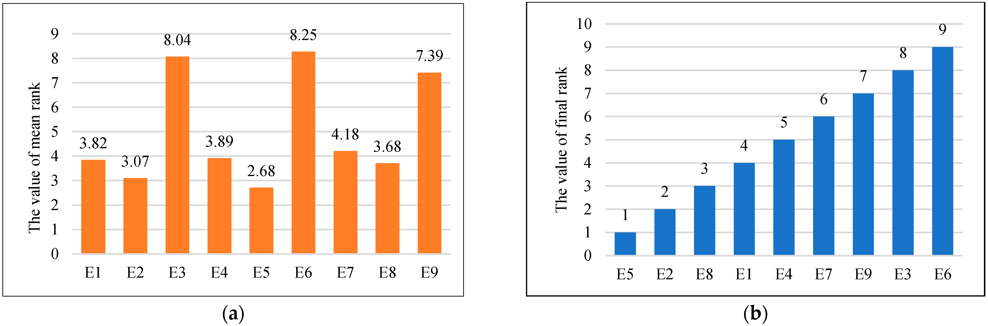
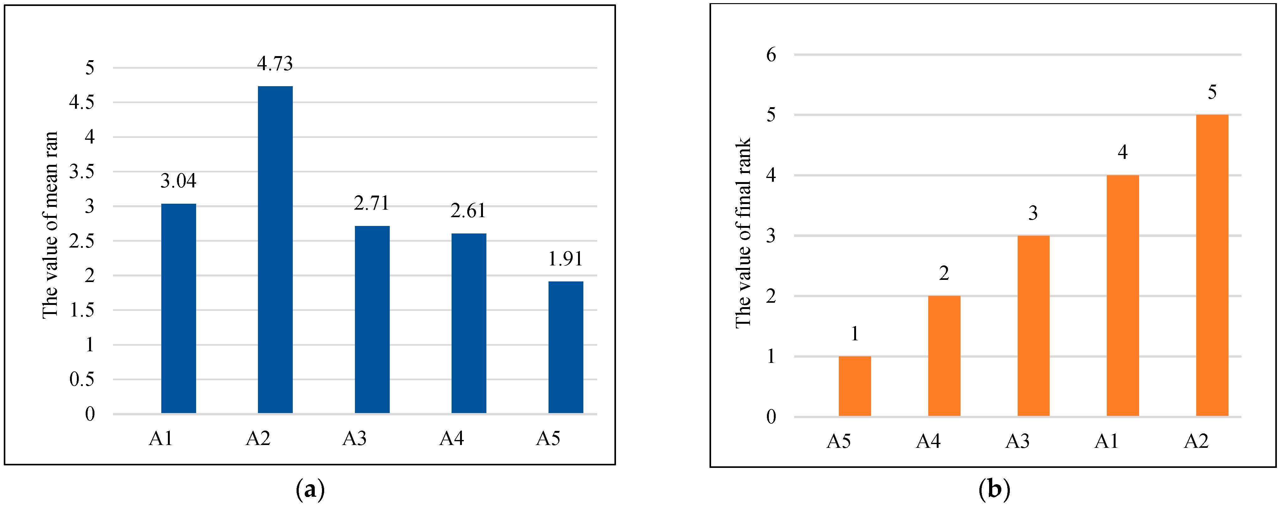
  • For each test function, all the algorithms participating in the comparison are sorted in the order of meanfij from small to large and give the algorithm rank ranking rankij (i = 1, 2, …, m; j = 1, 2, …, k). If the average value of the optimal value of the comparison algorithm is the same, then take the average of the ranking position as the rank ranking. To explain the calculation method of ranking and rank ranking, suppose there are five algorithms involved in the comparison. For a certain test function, if the average value of the optimal value obtained by the algorithm participating in the comparison is 1, 3, 3, 2 and 4, respectively, since the average of the optimal values found by the second and third algorithms are the same, then the ranking of the two algorithms are 3 and 4, respectively. Take the average of the ranking positions of these two algorithms ((3 + 4) / 2 = 3.5) as the rank ranking of the algorithm. Therefore, the rank rankings corresponding to the five algorithms are 1, 3.5, 3.5, 2 and 5. The results of the rank ranking are shown in Table 4.
  • Calculate the average of the rank ranking of each algorithm Averanki.
    A v e r a n k i = 1 m j = 1 k r a n k i j ( i = 1 , 2 ,   , m )
    where m is the number of participating comparison algorithms and k is the number of test functions.
  • Rank according to the average value Averanki of the rank ranking of each algorithm from small to large, the result of the sorting is the final ranking Finalranki of various algorithms.

4.2.2. Algorithm Performance Difference Significance Test

The Friedman test was first proposed by Friedman in 1945. It is a nonparametric test and is used to determine whether there are significant differences between the comparison algorithms. Suppose there are m comparison algorithms, that is, there are m samples. Each sample contains the average of the optimal value of the objective function obtained by k corresponding algorithms. Then, the Friedman test steps are as follows:
  • The original hypothesis, opposite hypothesis and significance level of Friedman test are given α.
H0: There is no significant difference in the performance of the m algorithms participating in the comparison;
H1: There are obvious differences in the performance of the m algorithms participating in the comparison.
2.
Calculate the rank of each algorithm corresponding to each test function rankji(1 ≤ Im, 1 ≤ jk).
3.
Calculate the sum of rank ranking of each test function corresponding to each algorithm sunranki; the sunranki calculation formula is sunranki:
s u n r a n k i = j = 1 k r a n k i j   ( i = 1 , 2 , , m )
4.
Calculate the Friedman test value χ2. The calculation formula of χ2 is:
χ 2 = 12 k m ( m + 1 ) i = 1 m s u n r a n k i 2 3 k ( m + 1 )
5.
According to the pre-determined significance level α and degrees of freedom (m − 1). Critical values can be obtained from the table of critical values of the Chi-square test χ2α[m − 1], if
χ 2 χ α ( m 1 ) 2
Then, reject the original hypothesis H0. It shows that there are obvious differences in the performance of the m algorithms participating in the comparison. Otherwise, accept the null hypothesis H0. It shows that there is no significant difference in the performance of the m algorithms involved in the comparison.

4.3. Obtain the Optimal Parameter Combination through Orthogonal Experiments

The best parameter combination can be found via orthogonal experiments because the threshold size and population size of the similarity-removal operation have a significant impact on algorithm performance. There are two factors in the orthogonal experiment, that is, the threshold ζ for the degree of similarity between individuals in the population and the population size n. Design three levels for each factor. The three levels of the threshold ζ are 0.3, 0.4 and 0.5; the three levels of population size are 0.95, 0.97 and 0.98. Therefore, the orthogonal experiment includes two factors and three levels. Table 5 and Table 6 show the orthogonal experimental design.
To obtain the optimal combination of parameters, the 30-dimensional CEC 2017 test function is selected. In addition, to ensure the fairness of the comparison results, suppose the population size n = 40, the dimension of the variable D = 30, maximum running time Maxtime = 20 s, the penalty factor M = 108, statistics times tjcs = 20. Table 7 and Table 8 and Figure 7 report the results of orthogonal experiments. The test results obtained are compared in Table 7. Table 8 exhibits the Friedman test results of the orthogonal experiment, and Figure 7 shows Friedman mean rank and final rank ranking.
In Table 8, χ2 = 160.54, χ2 α[k − 1] = 15.51. Since χ2χ2 α[k − 1], the original hypothesis is rejected. It shows that there are significant differences between the comparative test combinations. In addition, since E5 ranks first in all trial combinations (mean rank = 2.68), it shows that E5 is significantly better than other test combinations. Therefore, the optimal parameter combination is ζ = 0.4, P = 0.97.

4.4. Termination Condition of Algorithm Iteration

There are two commonly used iteration termination conditions at present. One is taking the maximum number of iterations as the termination condition and the other is taking the maximum evaluation times as the termination condition. However, the two iteration termination conditions are not fair to other algorithms participating in the comparison. The specific reasons are as follows:
  • Taking the maximum number of iterations as the iteration termination condition, it is unfair to the algorithms that participate in the comparison. Let the time required for an iteration of algorithm A be t1, the time required for one iteration of algorithm B is t2, and t1 > t2. Let t1 = 1.2t2, t2 = 0.005 s, the maximum number of iterations is 1000. When both algorithm A and algorithm B reach the maximum number of iterations, algorithm A needs 6 s and algorithm B needs 5 s. The running time of A is 1 s longer than the running time of B. If the solution quality of A is better than that of B, it cannot be said that the performance of algorithm A is better than that of algorithm B. Because the running time of A is long, if algorithm B runs for another 1 s, the quality of the solution from algorithm B is not necessarily worse than that of algorithm A.
  • Taking the maximum evaluation times of the objective function as the termination condition of the algorithm iteration, it is also unfair to the algorithms involved in the comparison. The main reasons are: some algorithms in an iteration process, although the evaluation times of the objective function are few, the running time of the program is very long; some algorithms in an iteration process, although there are many evaluation times of the objective function, but the running time of the program is very short. Therefore, taking the maximum evaluation times of the objective function as the iteration termination condition is unfair to some algorithms.
In summary, to fairly compare various algorithms, the maximum running time Maxtime can be used as the iteration termination condition of the algorithm. Therefore, Maxtime is taken as the termination condition of algorithm iteration in this paper. When the program’s running time reaches Maxtime, the algorithm stops iterating and outputs the optimal solution and value. The advantages of taking the maximum running time Maxtime as the termination condition of algorithm iteration are: regardless of whether the time and space complexity of different algorithms are the same, it is fair to the algorithms participating in the comparison.

4.5. Performance Comparison of Different Attraction Models

To verify that the performance of the probability attraction model is better than other attraction models, the CAM, RAM, NAM and GAM were selected to compare their performance with the probability attraction model. In addition, to ensure the fairness of the comparison, IHFAPA uses a different model of attraction and the rest is the same. Suppose population size n = 40, dimension of variable D = 30, maximum running time Maxtime = 20 s, maximum attraction βmax = 1, minimum attraction βmin = 0.5, light-absorption coefficient γ = 1, penalty factors corresponding to equality constraints and inequality constraints M1 = M2 = 108. The test function is CEC 2017; IHFAPA with different attractors was independently run 20 times. Run 20 times independently to obtain the mean value of the optimal value of the test function and the standard deviation of the optimal value, as shown in Table 9. The results of Friedman’s mean rank and final rank ordering for different attraction models are given in Figure 8. The Friedman test results of different attraction models are shown in Table 10.
In Table 9, Mean is the average value of the optimal value of the test function obtained when each test function runs 20 times and Std is the standard deviation for the optimal value obtained. Table 9 indicates that the probability attraction model performs better than the other attraction models in regard to winning frequency. As a result, the probability attraction model performs significantly better than other attraction models. Figure 8 demonstrates that the probability attraction model performs better than the other attraction models that were tested by placing first in both the mean rank and final rank among all the attraction models that were compared. In addition, Friedman test was selected to verify whether there were noticeable differences in the performance of the various attraction models involved in the comparison. According to Table 10, when k = 5, α = 0.05, χ2α[4] the degree of freedom k − 1 = 4 corresponds toχ2α[4] = 9.49, χ2 = 26.07, χ2 > χ2α[4]. Therefore, rejecting the original hypothesis shows that there are obvious differences in the performance of various attraction models involved in the comparison.
In conclusion, for the 28 30-D test functions in CEC 2017, the performance of the probabilistic attraction model is better than the other four models, which verifies the validity of the probabilistic attraction model.

4.6. Performance Comparison between IHFAPA and Other FAs

To verify the superiority of the IHFAPA algorithm, five different FA algorithms were selected for comparison. The selected algorithm is:
  • Standard firefly algorithm (SFA) [6];
  • Random-attracting firefly algorithm (RaFA) [19];
  • Neighborhood-attracting firefly algorithm (NaFA) [42];
  • Gender-difference firefly algorithm (GDFA) [47];
  • An adaptive Log Spiral levy firefly algorithm (ADIFA) [29];
  • Cauchy mutation of the Yin and Yang firefly algorithm (YYFA) [36];
  • Group-attraction hybrid firefly algorithm (GAHFA) [20].

4.6.1. Parameter Settings

To compare the performance of various algorithms fairly, suppose the population size of all algorithms is n = 40, maximum running time Maxtime = 20 s, penalty factor M = 108, the allowable error value of the equality constraint for constrained optimization problem θ = 10−4 and number of statistics tjcs = 20. The other parameters in the comparison algorithm adopt the values in the original literature, and the specific parameter values are shown in Table 11.

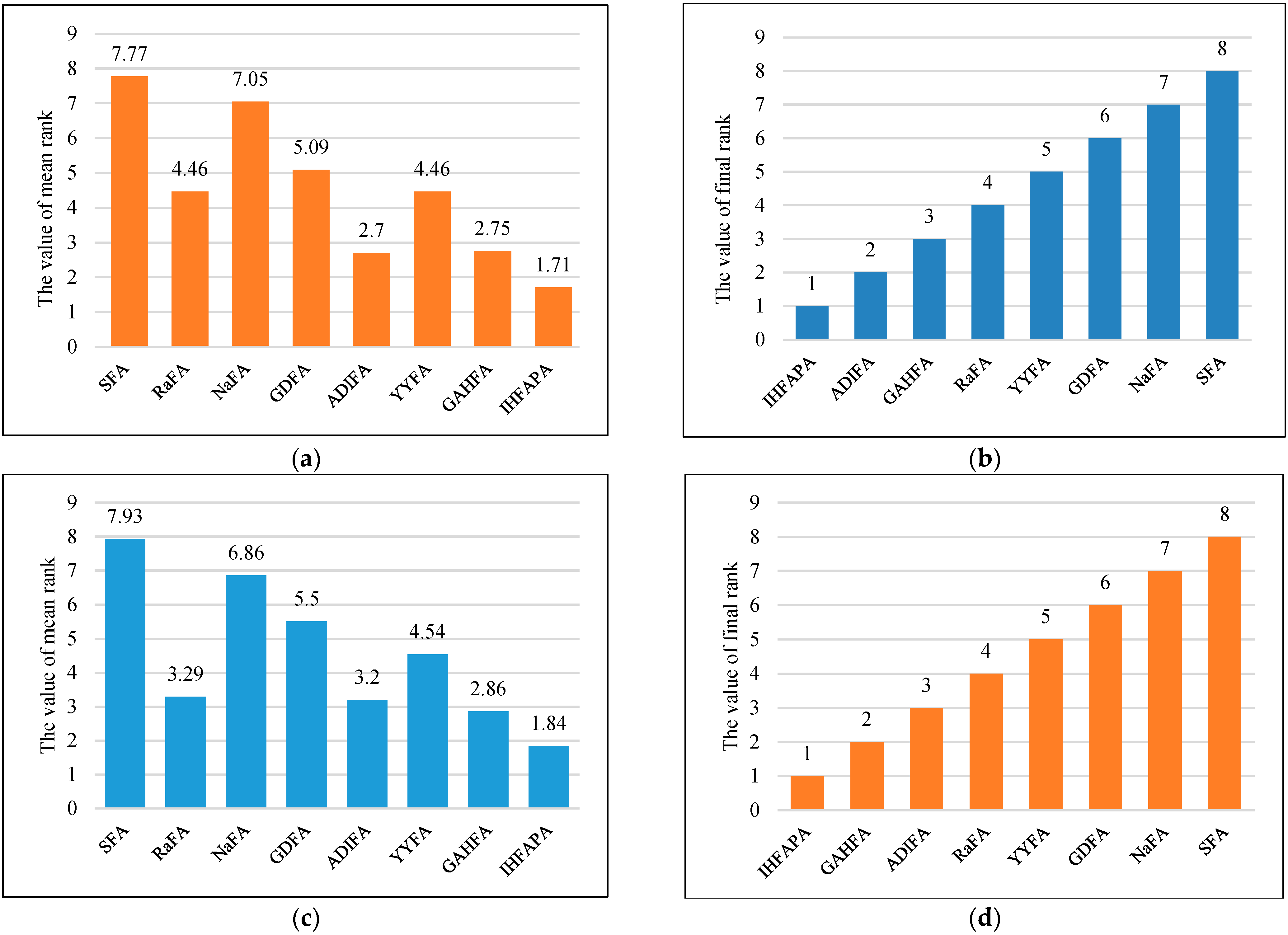
4.6.2. Statistical Results and Analysis

  • Statistical results
Calculation results of 28 benchmark functions in CEC 2017 of various firefly algorithms D = 30 and D = 50 are given in Table 12 and Table 13, and the Friedman test results are shown in Table 14 and Table 15. Holm’s procedure was used to further verify the algorithm performance. The results of all pairwise comparisons are summarized in Table 16 and Table 17. When D = 30 and D = 50, the ranking results of the Friedman average rank and final rank of various FA algorithms are shown in Figure 9.
2.
Result analysis
(1) Analysis of the calculation results of the 30-D test function
Figure 9 reports that, when using the eight firefly algorithms to solve the C03 benchmark test function, GDFA produces the highest-quality solutions; similarly, YYFA produces the highest-quality results when addressing the two C13 and C25 benchmark test functions. The highest quality of the ADIFA solutions is achieved when solving the six test functions C07, C15, C16, C17, C24 and C26; when solving the other 19 benchmark functions, IHFAPA has the highest solution quality. According to the w/t/l values in Table 12, IHFAPA has better performance than the seven other firefly algorithms. Specifically, IHFA-PA has 28 test functions with a mean value better than SFA, 27 test functions with a mean value better than RaFA, 28 test functions with a mean value better than NaFA, 28 test functions with a mean value better than NDFA and for 27 test functions, the mean is better than GDFA, the mean of 25 test functions is better than YYFA and the mean of 22 test functions is better than AD-IFA. From the Friedman ranking results of various FAs with D = 30 in (a) and (b) of Figure 9, IHFAPA ranks first among all the algorithms, indicating that IHFAPA’s performance is superior to the comparison algorithm in this paper. In addition, the Friedman test was used to verify whether there were obvious differences in the performance of the various algorithms involved in the comparison. In Table 13, k = 8, α = 0.05, k – 1 = 7, the critical value χ2α[7] = 14.07, inspection value χ2 = 148.47 and the inspection value χ2 is greater than the critical value χ2α[7], so the null hypothesis is rejected, indicating that there are obvious differences in the performance of the eight algorithms. From Table 14, the results obtained from Holm’s procedure show that the IHFAPA did not show a significant difference from the GAHFA for the adjusted p-value and unadjusted p-value, but IHFAPA is significantly due to GAHFA in other indicators. Compared to NaFA, RaFA, NDFA, GDFA, AD-IFA and YYFA, IHFAPA verified the algorithm’s superior performance. The statistical test shows that the IHFAPA was significantly different from the other comparison algorithms, with all p-values less than 0.05 at a 95% confidence level. The analyses above demonstrate the outstanding performance of the IHFAPA.
In summary, the experimental results of 28 30-D test functions in CEC 2017 show that the outperformance of IHFAPA over the other seven FAs verifies the effectiveness of IHFAPA.
(2) Analysis of calculation results of 50-D test function
Table 15 demonstrates that RaFA has the highest solution quality when eight firefly algorithms are used to solve the C06 benchmark function, GDFA has the highest solution quality when to solve the C03 and C25 benchmark functions, ADIFA has the highest solution quality when five test functions—C13, C15, C16, C24 and C26—are solved and IHFAPA has the highest solution quality when solving the remaining 20 benchmark functions. Figure 9’s (c,d) results show that IHFAPA performs better than the other seven firefly algorithms. Specifically, IHFA-PA has 28 test functions with a mean value better than SFA, 25 test functions with a mean value better than RaFA, 28 test functions with a mean value better than NaFA, 28 test functions with a mean value better than NDFA, 26 test functions with an average value better than GDFA, the average value of 28 test functions is better than YYFA and the average value of 22 test functions is better than AD-IFA. It can be seen from Table 15 that IHFAPA ranks first among all algorithms, indicating that IHFAPA’s performance is superior to other algorithms involved in the comparison. In addition, Friedman test is used to verify whether there is a significant difference in the performance of the eight algorithms. According to Table 16, inspection value χ2 = 151.31, when k = 8, α = 0.05, k − 1 = 7, the critical value χ2α[7] = 14.07. Because the inspection value χ2 is greater than the critical value χ2α[7], the original hypothesis is rejected, showing that there are significant differences in the performance of the eight algorithms. From Table 17, the results obtained from Holm’s procedure show that the IHFAPA did not show a significant difference from the GAHFA for the adjusted p-value and unadjusted p-value, but IHFAPA is significantly superior to GAHFA in other indicators. IHFAPA confirmed the algorithm’s superior performance when measured against the other comparative algorithms. The statistical test demonstrates that the IHFAPA differed from the other comparison algorithms in a significant way.
In summary, the experimental results of 28 50-D test functions in CEC 2017 show that the performance of IHFAPA is better than the other seven firefly algorithms, thus, verifying the effectiveness of IHFAPA.

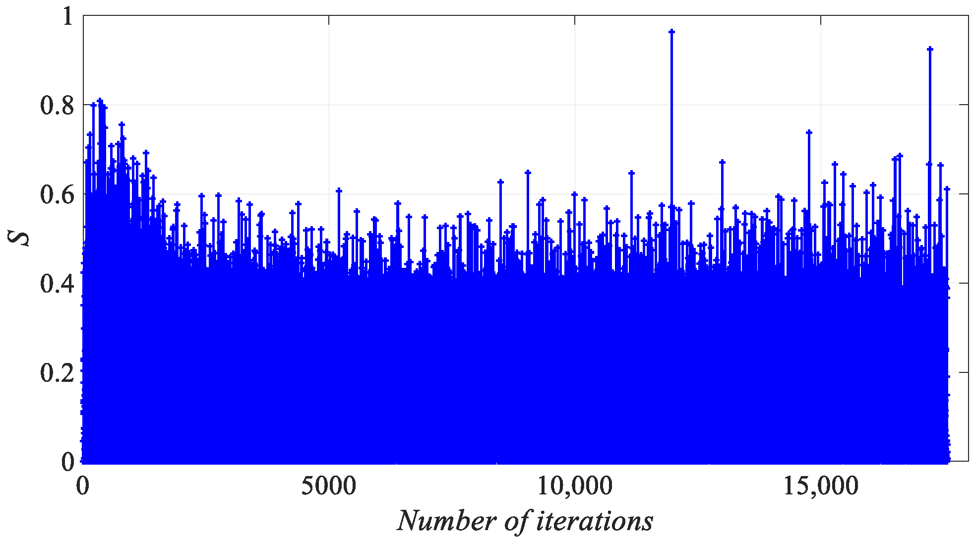
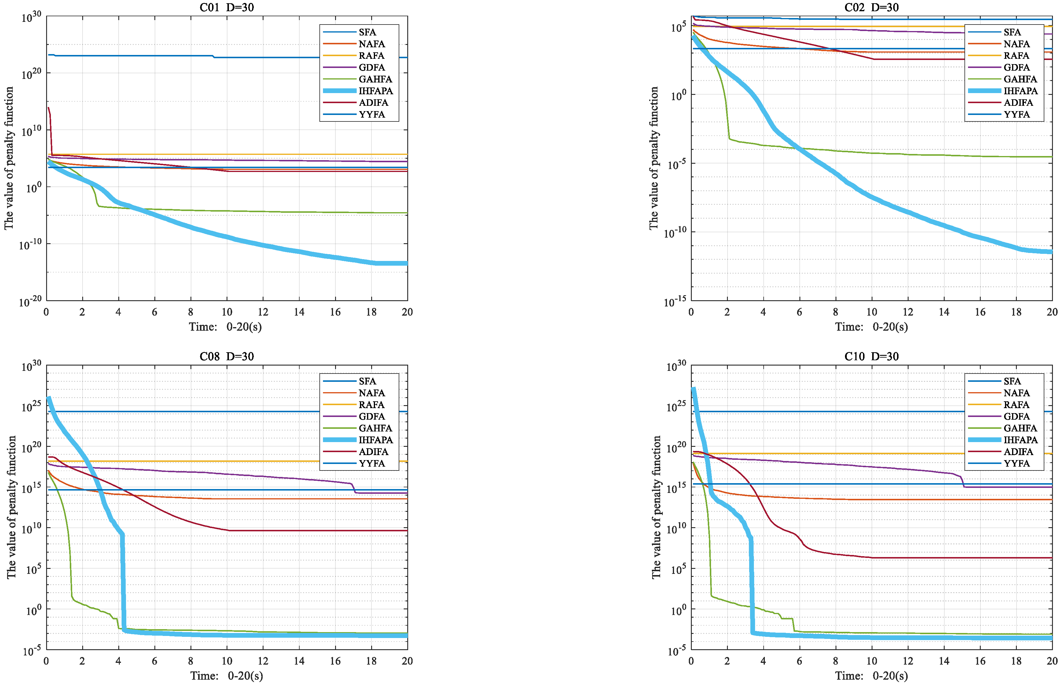
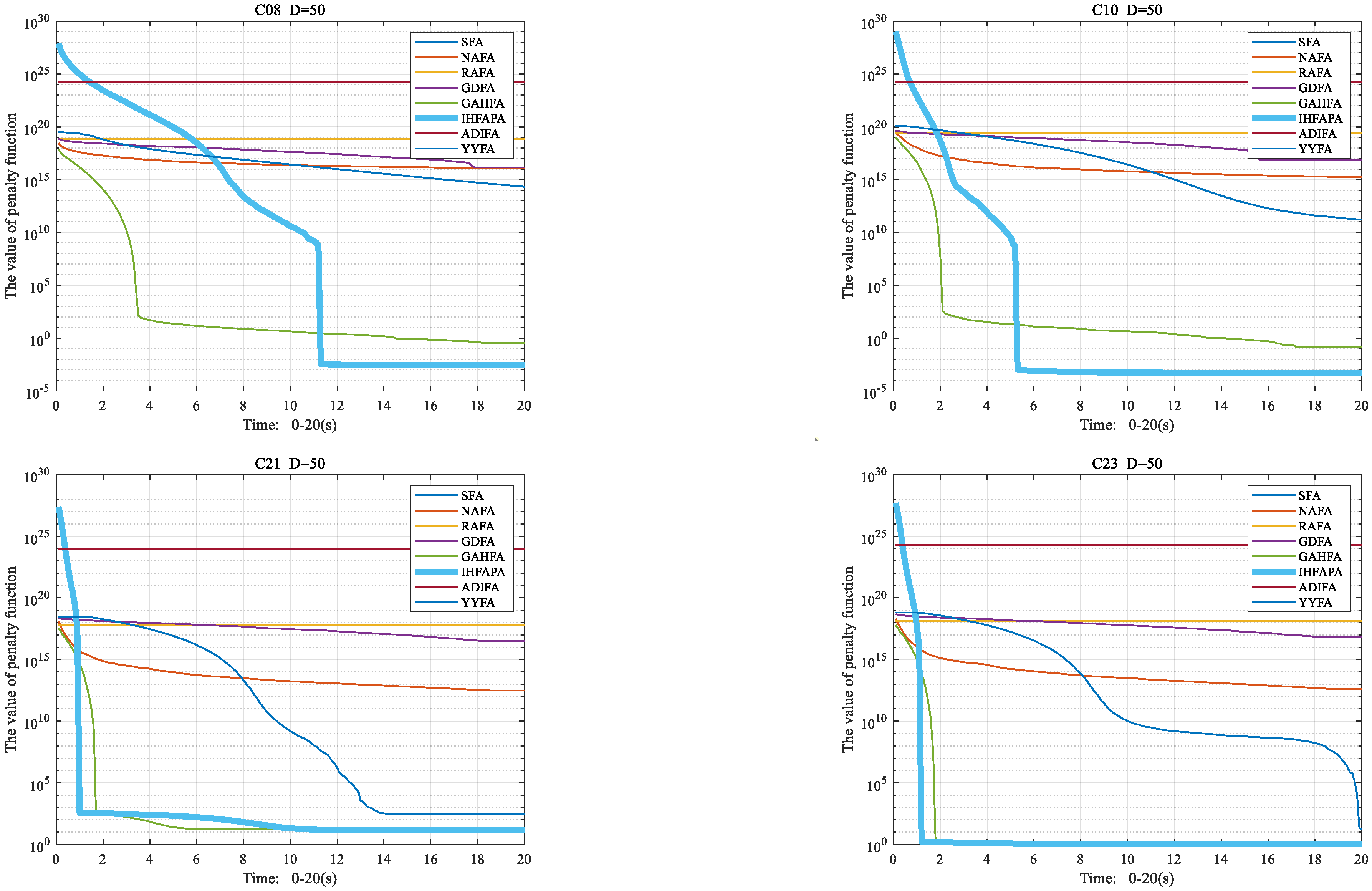
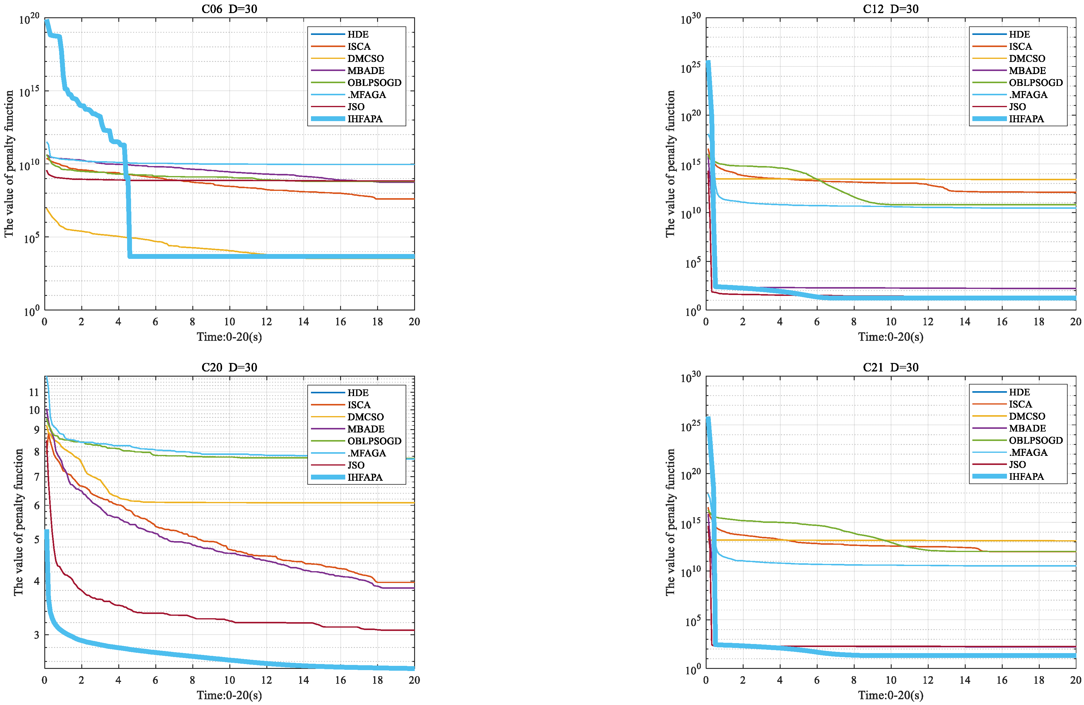
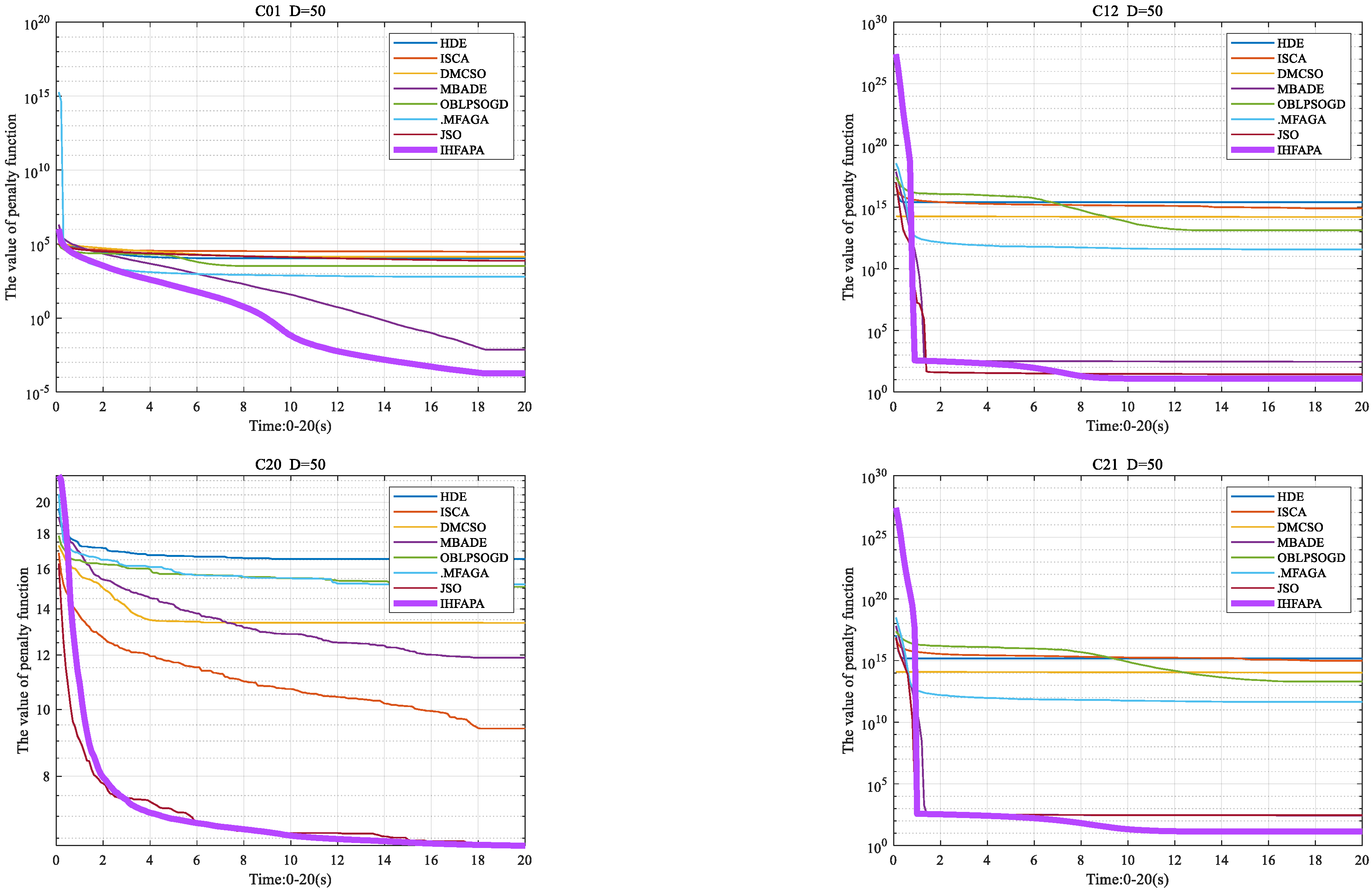
4.6.3. Convergence Curve of Firefly Algorithm

To verify that IHFAPA’s performance is superior to other FAs, four 30-D and 50-D test functions in CEC 2017 are selected and draw the convergence curves of eight FAs. The convergence curve of FA for solving four 30-D test functions is shown in Figure 10, and the convergence curve of FA for solving four 50-D test functions is shown in Figure 11.
According to Figure 10, for C01 and C02, IHFAPA converges to the global optimal solution much more quickly than the other six algorithms, with the exception of GAHFA, at the beginning of the iteration. At the end of the iteration, IHFAPA uses the combined mutation operator and adds the de-similarity operation, giving it a strong exploration ability. Therefore, IHFAPA has better solving quality than the other seven algorithms. For C08 and C10, the convergence speed of IHFAPA and GAHFA is obviously better than the other six algorithms. At the end of the iteration, IHFAPA and GAHFA rapidly converge to the global extreme point, while the other six algorithms fall into local optimum. In addition, IHFAPA’s solution accuracy is superior to GAHFA due to its strong exploitation ability.
Figure 11 illustrates, for C08 and C10, that IHFAPA and GAHFA converge faster than the other six algorithms in the early iteration; in late iterations, IHFAPA uses a combined mutation operator and adds the remove-similarity operation, so IHFAPA has strong exploration ability and can quickly move closer to the global optimal advantage, while the other seven algorithms have relatively weak exploration ability and quickly fall into local optimum. Therefore, IHFAPA’s convergence speed and solving quality are better than those of the other seven algorithms. For C21 and C23, the convergence speed of IHFAPA and GAHFA is better than the other six algorithms in the early iteration stage; at the end of the iteration, except IHFAPA and GAHFA, the other six algorithms quickly fall into local optimum, while IHFAPA and GAHFA approached the global optimum quickly. In summary, IHFAPA is superior to other algorithms in convergence speed and solution quality.

4.7. Comparison of IHFAPA and Other Improved Algorithms

To further verify the performance of the IHFAPA, we selected six other improved algorithms for comparison. The six other improved algorithms selected are as follows:
  • Adaptive differential evolution algorithm (HDE) [47];
  • Improved sine and cosine algorithm with crossover operator (ISCA) [48];
  • Hybrid chicken swarm algorithm based on differential mutation (DMCSO) [49];
  • Particle swarm optimization based on oppositional group decision learning (OBLPSOGD) [50];
  • Hybrid algorithm of improved bat algorithm and differential evolution algorithm (MBADE) [51];
  • Firefly single-objective genetic optimization algorithm based on partition and unity (MFAGA) [52];
  • Single-objective real-parameter optimization: Algorithm Jso (JSO) [53];
Select 28 test functions in CEC 2017 to compare the performance of IHFAPA, HDE, ISCA, DMCSO, OBLPSOGD, MBADE, MFAGA and JSO.

4.7.1. Parameter Setting

To compare the performance of various algorithms fairly, the population size of all algorithms n = 40, the maximum running time Maxtime = 20 s, the penalty factor M1 = M2 = 108, the allowable error of equality constraints in constraint optimization problem θ = 10−4 and the statistical times tjcs = 20. The values in the original literature were used for the other parameters of the comparison algorithm, and the specific parameter values are shown in Table 18.

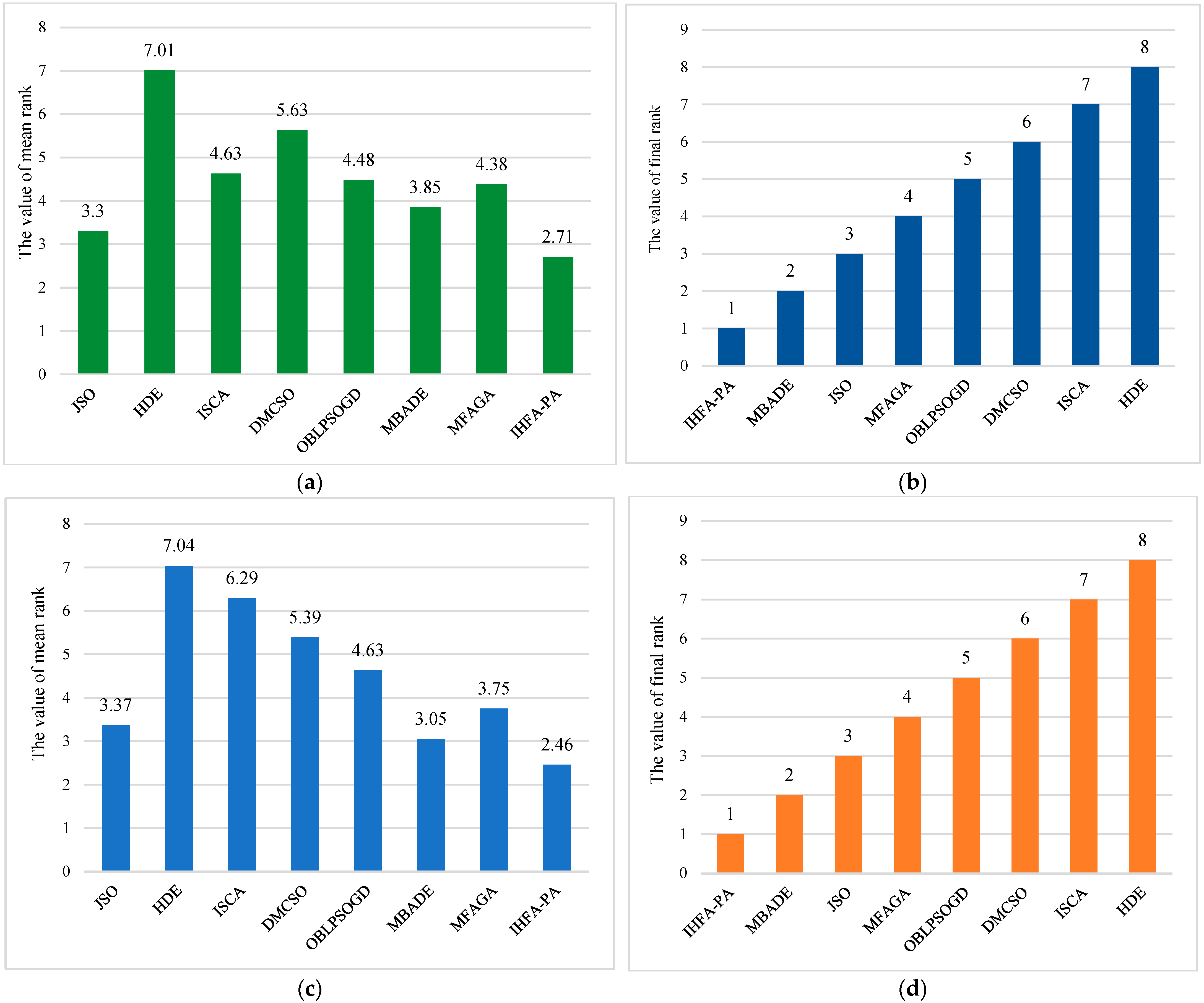
4.7.2. Statistical Results and Analysis

1.
Statistical results
When the variable dimension D = 30 and D = 50 of the 28 benchmark test functions in CEC 2017, the statistical results of the seven meta-heuristic algorithms are reported in Table 19 and Table 20, the results of Friedman rank ranking are shown in (a) and (b) in Figure 12 and the results of Friedman test are shown in Table 21 and Table 22. Holm’s post hoc pairwise comparison results are in Table 23 and Table 24.
2.
Results analysis
(1) Analysis of the results of 30-D test functions
From Table 19, JSO obtains the optimal solution in the three test functions of C10, C11 and C22. When solving the benchmark functions C03, C06 and C28, DMCSO has the highest solution quality, whereas ISCA has the highest solution quality for C09 and C13. With regard to the five benchmark functions C07, C15, C16, C24 and C25, OBLPSOGD has the best solution quality. When solving the C19 benchmark function, MBADE has the highest solution quality. The solution quality of IHFAPA is the highest when the fourteen test functions C01, C02, C05, C08, C12, C14, C17, C18, C20, C21, C23, C26 and C27 are solved. Figure 12a,b show that IHFAPA ranks first among the seven meta-heuristic algorithms, indicating that IHFAPA’s performance is better than the other seven meta-heuristic algorithms. In addition, Friedman test is used to verify whether there is a significant difference in the performance of the seven algorithms. According to Table 20, k = 8, α = 0.05, k − 1 = 7, critical value χ2α[6] = 14.07 and inspection value χ2 = 118.68. Because the test value is greater than the critical value, the null hypothesis is rejected, showing that there are obvious differences in the performance of the seven algorithms. Table 21 reports that Holm’s experimental results show that IHFAPA only shows no significant difference with JSO in the adjusted p-value and the unadjusted p-value, but IHFAPA is significantly better than JSO in other indicators. Statistical tests show that IHFAPA is significantly different from other comparison algorithms.
In conclusion, the experimental results of 28 30-D test functions in CEC 2017 show that IHFAPA performs better than the other seven meta-heuristic algorithms, thus, verifying the effectiveness of IHFAPA.
(2) Analysis of the results of 50-D test functions
Table 22 reports that JSO has the highest solution quality for C04, C15 and C18 benchmark functions; OBLPSOGD has the highest solution quality when solving C17 and C18 benchmark functions with seven meta-heuristic algorithms; MBADE has the highest solution quality when solving the eight benchmark functions C03, C05, C07, C16, C19, C22, C25 and C27; when solving the C28 benchmark test function, MFAGA has the highest solution quality; IHFAPA’s C01, C02, C04, C08, C09, C10, C12, C14, C20, C21, C23, C24 and C26 benchmark functions have the highest solving quality. According to the w/t/l values in Table 22, IHFAPA’s performance is better than the other meta-heuristic algorithms. Specifically, IHFA-PA has 25 test functions with a mean value better than JSO, 28 test functions with a mean value better than HDE, 28 test functions with a mean value better than ISCA, 28 test functions with a mean value better than DMCSO, 23 test functions with a mean value better than OBLPSOGD and 18 test functions with a mean value better than MBADE; the average of 26 test functions is better than MFAGA. In Figure 12, (c) and (d) show that IHFAPA ranks first among the seven meta-heuristic algorithms, indicating that IHFAPA’s performance is better than the other six meta-heuristic algorithms. In addition, Friedman test is used to verify whether there is a significant difference in the performance of the seven algorithms. According to Table 23, k = 7, α = 0.05, k − 1 = 6, critical value χ2α[6] = 12.59 and inspection value χ2 = 75.75. Since the test value is greater than the critical value, the null hypothesis is rejected, showing that there are obvious differences in the performance of the seven algorithms. From Table 24, Holm’s experimental results show that IHFAPA only shows no significant difference with MBADE in the adjusted p-value and the unadjusted p-value, but IHFAPA is significantly better than MBADE in other indicators. Statistical tests show that IHFAPA is significantly different from other comparison algorithms.
In conclusion, the experimental results of 28 50-D test functions in CEC 2017 show that IHFAPA performs better than the other seven meta-heuristic algorithms, thus, verifying the effectiveness of IHFAPA.

4.7.3. Convergence Curve of the Proposed Algorithm

The results of IHFAPA’s better performance than the other six meta-heuristic algorithms were visualized. Four 30-D and 50-D test functions of CEC 2017 are selected to draw convergence curves of eight FAs. Convergence curves of FA solving four 30-D test functions are shown in Figure 13, and convergence curves of FA solving four 50-D test functions are shown in Figure 14.
In Figure 13, for C06, the convergence speed of IHFAPA is like that of DMCSO, and the solution accuracy of the two is better than other proposed comparison algorithms. For C12 and C21, the convergence speed of IHFAPA and MBADE is faster than that of other proposed algorithms in the early stage of iteration; however, due to the usage of a combined mutation operator and the addition of a removing-similarity operation, IHFAPA has great exploration ability in the late stage of iteration and can jump out of the local optimal value and swiftly converge to the global optimal value. IHFAPA, therefore, handles quality problems better than the other six algorithms. IHFAPA clearly outperforms other algorithms in terms of solution quality for C20 and has a rapid convergence speed in the initial iteration.
Figure 14 illustrates that when calculating the 50-D CEC2017 test function, C01 test function converges to the optimal value of the solution faster than the other seven functions in the early stage, showing that IHFAPA has strong global search ability. In the C12 test function, IHFAPA has a fast convergence speed in the early stage of search, similar to MBADE and ILTD-ABC, but the solution accuracy of IHFAPA is higher than that of the other seven algorithms in the late stage of the search process. For C12 and C21 test functions, IHFAPA’s convergence speed is relatively fast in the early stage of the search for the two test functions, but for the C21 test function, IHFAPA’s solution accuracy is better in the later stage of the search and other algorithms fall into local optimum, which shows that IHFAPA has a strong ability to jump out of local optimum.

5. Application to Engineering Problems

To further verify the effectiveness of IHFAPA, 14 intelligence optimization algorithms in the literature were selected, namely, SFA [6], RaFA [19], NaFA [43], GDFA [49], ADIFA [29], YYFA [36], GAHFA [20], HDE [47], ISCA [48], DMCSO [49], OBLPSOGD [50], MBADE [51], MFAGA [52] and JSO [53]. Then, 14 meta-heuristic algorithms in IHFAPA and the literature were used to solve the optimization design problems for the cantilever beam, welded beam, piston rod and three-bar truss, and the results of 14 intelligence optimization algorithms were counted and compared.
Set the population size n = 40, the maximum running time Maxtime = 20 s, the penalty factor M1 = M2 = 108 and the allowable error values for equality constraint in constrained optimization problems θ = 10−4 in order to accurately compare the performance of various algorithms. For each engineering optimization problem, each algorithm is run 20 times independently, the results are solved statistically and the results are compared and analyzed to verify the effectiveness and feasibility of IHFAPA in practice.

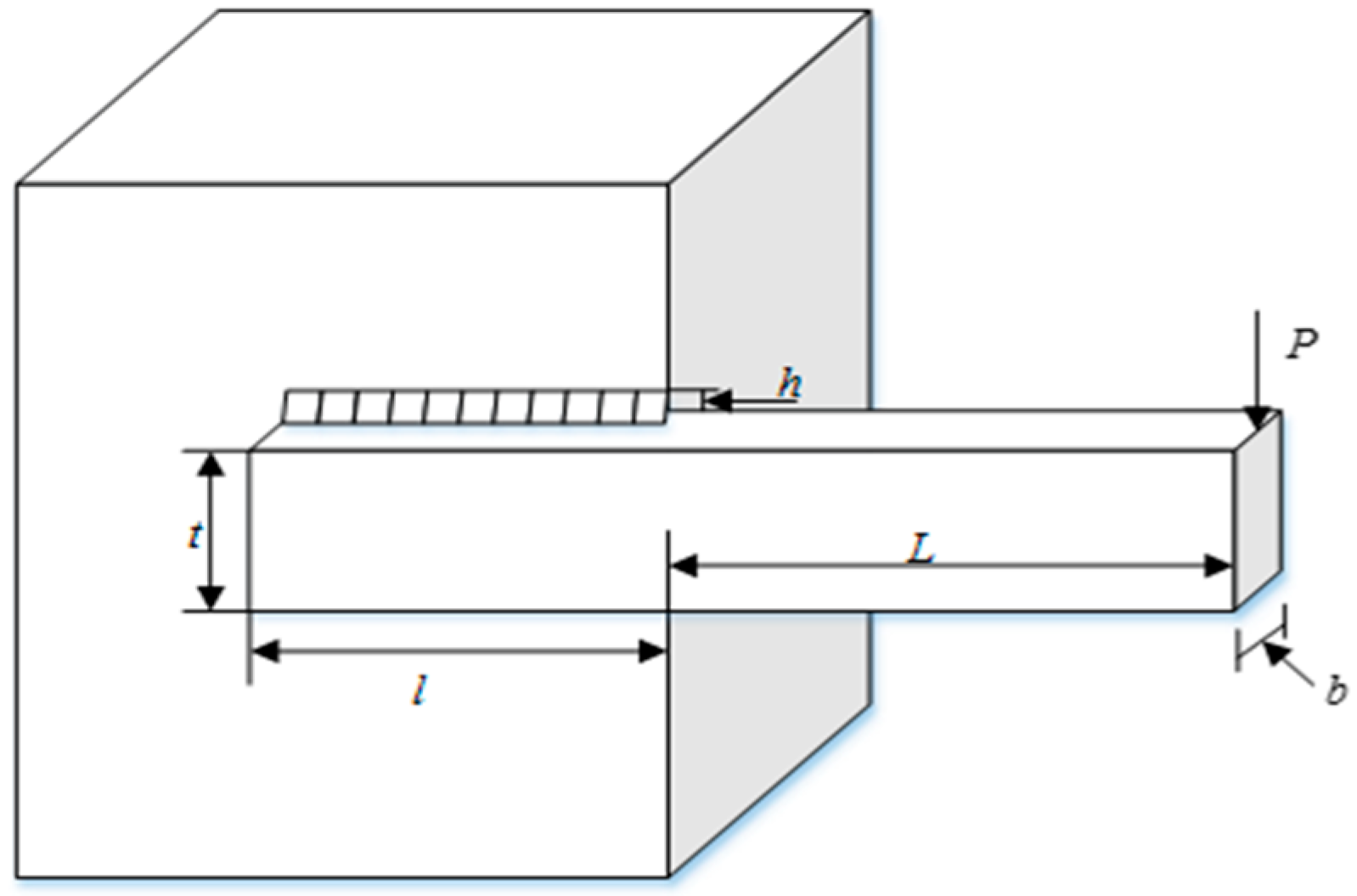
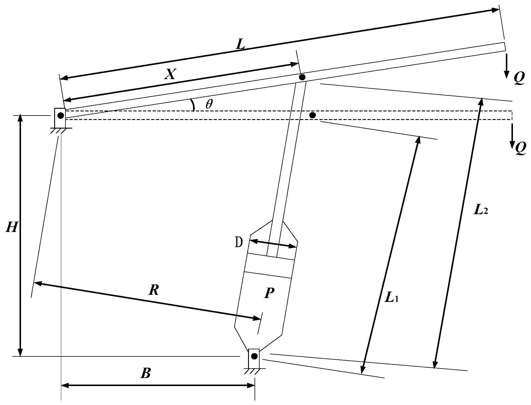
5.1. Optimization Design of Cantilever Beam [28]

The aim of the cantilever beam design is to minimize the weight of the cantilever beam. Taking the optimization design of the cantilever beam given in the literature [28] as an example, the cantilever beam structure is shown in Figure 15.
The mathematical model for the optimal design of the cantilever beam is as follows:
min f ( X ) = 0.6224 ( x 1 + x 2 + x 3 + x 4 + x 5 ) s . t . { g ( X ) = 61 x 1 3 + 27 x 2 3 + 19 x 3 3 + 7 x 4 3 + 1 x 5 3 1 0 0.01 x 1 , x 2 , x 3 , x 4 , x 5 100
Table 25 shows that 14 intelligence optimization algorithms are used to solve Equation (13) and the best result of various algorithms solving Problem 1. To better evaluate the performance of the algorithm, the minimum optimal value (Best), maximum optimal value (Worst), average optimal value (Mean) and standard deviation of optimal value (Std) are taken as statistical indicators. Table 26 gives the statistical indicator values of the algorithms.
In Table 25, the optimal value obtained by MFAGA and IHFAPA is the smallest among the 14 algorithms. Table 26 illustrates that the Best, Worst, Mean and Std of IHFAPA and MFAGA are the same and better than the other 11 algorithms. Therefore, the quality of IHFAPA is not inferior to the other algorithms in solving the cantilever optimization design problem, which verifies the effectiveness of IHFAPA.

5.2. Optimization Design of Welded Beam [54]

One well-known nonlinear optimization design problem in the realm of engineering is the optimization of welded beams. The objective of this problem is to minimize the manufacturing cost of welded beams under the constraints of shear stress (τ), beam end deflection (δ), bar buckling load (Pc) and bending stress (σ). The design variable for the optimization design of the welded beam is X = [x1,x2,x3,x4]. The structure of the welded beam is shown in Figure 16.
The mathematical model for the optimization design of the welded beam is:
min   f ( X ) = 1.10471 x 1 2 x 2 s . t . { g 1 ( X ) = τ ( x ) τ max 0 g 2 ( X ) = σ ( x ) σ max 0 g 3 ( X ) = δ ( x ) δ max 0 g 4 ( X ) = x 1 x 4 0 g 5 ( X ) = P P c ( x ) 0 g 6 ( X ) = 0.125 x 1 0 g 7 ( X ) = 1.10471 x 1 2 + 0.04811 x 3 x 4 ( 14.0 + x 2 ) 5.0 0
τ ( X ) = ( τ ) 2 + 2 τ τ x 2 2 R + ( τ ) 2
τ = P 2 x 1 x 2
τ = MR J
M = P ( L + x 2 2 )
R = x 2 2 4 + ( x 1 + x 3 2 ) 2
J = 2 { 2 x 1 x 2 [ x 2 2 4 + ( x 1 + x 3 2 ) 2 ] }
σ ( X ) = 6 P L x 4 x 3 2
δ ( X ) = 6 P L 3 E x 3 2 x 4
P c ( x ) = 4.013 E x 3 2 x 4 6 36 L 2 ( 1 x 3 2 L E 4 G )
where P = 6000 lb, τmax = 13600 psi, δmax = 0.25 in, L = 14 in, E = 30 × 106 psi, G = 12 × 106 psi and σmax = 30,000 psi.
The value range of design variables in the optimization design of welded beams is 0.1 ≤ xi(i = 1,4) ≤ 2, 0.1 ≤ xi (i = 2,3) ≤ 10. Table 27 reports intelligence optimization algorithms are used to solve Equation (34) and the best result of various algorithms solving Problem 2. To better evaluate the performance of the algorithm, the Best, Worst, Mean and Std are taken as statistical indicators. The statistical indicator values of the 14 algorithms are given in Table 28.

5.3. Optimization Design of Piston Rod [55]

The piston rod structure is also a common optimization structure in practical engineering, and its structure is shown in Figure 17.
The primary objective of the piston rod optimization problem is to position piston components H, B, D and X by minimizing the amount of oil when the piston rod moves from 0 to 45°.
The design variable of the piston rod optimization problem is X = [H, B, D, X] = [x1, x2, x3, x4] and the mathematical model is:
min f ( X ) = 1 4 π x 4 2 ( L 2 L 1 ) s . t . { g 1 ( X ) = Q L cos θ R F 0 g 2 ( X ) = Q ( L x 4 ) M max 0 g 3 ( X ) = 1.2 ( L 2 L 1 ) L 1 0 g 4 ( X ) = x 3 / 2 x 2
R = | x 4 ( x 4 sin θ + x 1 ) + x 1 ( x 2 x 4 cos θ ) | ( x 4 x 2 ) 2 + x 1 2
F = π P x 3 2 4
L 2 = ( x 4 sin θ + x 1 ) 2 + ( x 2 x 4 cos θ ) 2
L 1 = ( x 4 x 2 ) 2 + x 1 2
where Q = 10,000 lbs, θ = 45°, L = 240 in, oil pressure P take 1500 psi and maximum allowable bending moment of lever Mmax = 1.8 × 10⁶ lbs in.
The design variable of the piston lever optimization design problem ranges from 0.05 ≤ xi(i = 1,2,3) ≤ 500 to 0.05 ≤ x4 ≤ 120. Thus, 13 intelligence optimization algorithms are used to solve Equation (44) and the best result of various algorithms solving Problem 3 is reported in Table 29. In order to better evaluate the performance of the algorithm, Best, Worst, Mean and Std are taken as statistical indicators. The statistical indicator values of the 13 algorithms are given in Table 30.

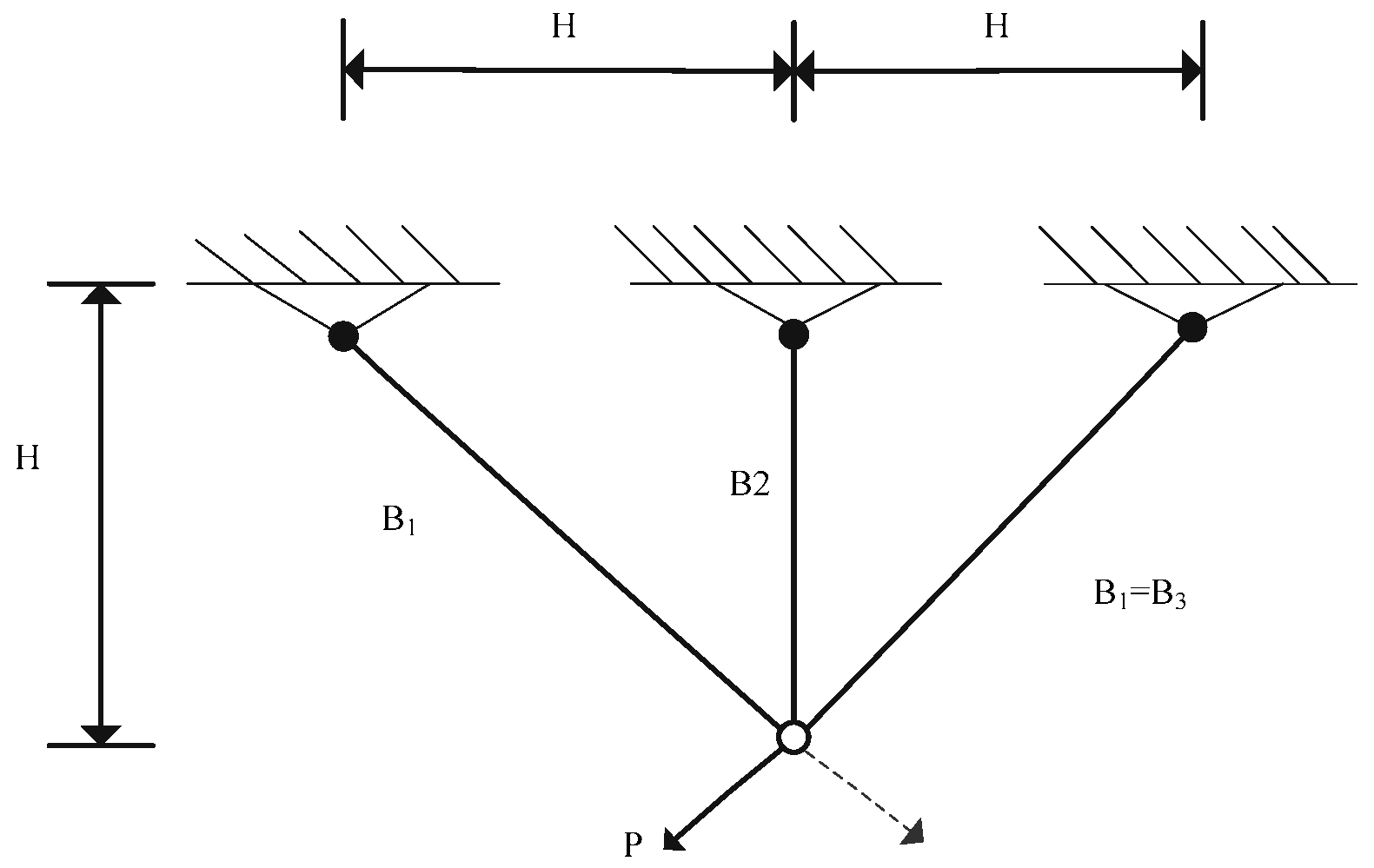
5.4. Optimization Design of Three-Bar Truss [55]

The three-bar truss structure is shown in Figure 18.
The objective of the optimization design of the three-bar truss is to minimize the weight of the three-bar truss under the constraints of stress, deflection and buckling. The design variable of the optimization design of the three-bar truss is [B1, B2] = [x1, x2]. The mathematical model of the optimization problem is:
{ min f ( X ) = 100 ( 2 2 x 1 + x 2 ) s . t .   { g 1 ( x ) = 2 ( 2 x 1 + x 2 ) / ( 2 x 1 2 + 2 x 1 x 2 ) 2 0 g 2 ( x ) = 2 x 2 / ( 2 x 1 2 + 2 x 1 x 2 ) 2 0 g 3 ( x ) = 2 / ( 2 x 2 + x 1 ) 2 0
The value range of design variables for the optimization of the three-bar truss design is as follows: 0 ≤ x1 ≤ 1 and 0 ≤ x2 ≤ 1. Table 31 reports that 14 intelligence optimization algorithms are used to solve Equation (49) and the best result of various algorithms solving Problem 4. To better evaluate the performance of the algorithm, Best, Worst, Mean and Std are taken as statistical indicators. The statistical indicator values of the 14 algorithms are given in Table 32.
According to Table 31, the Best of IHFAPA is the smallest among 14 algorithms. From Table 32, the Best, Worst, Mean and Std of IHFAPA are better than the other algorithms. Therefore, IHFAPA is superior to the other algorithms in solving the optimization design problem of the three-bar truss, thus, verifying the effectiveness of IHFAPA.
In summary, the optimization results of the four engineering optimization problems show that the minimum optimal value obtained by IHFAPA is better than other algorithms when solving piston rod optimization design problems, and the standard deviation of maximum optimal value, average optimal value and optimal value obtained by IHFAPA is not worse than that of the other algorithms. When the 14 algorithms solve the cantilever beam optimization design problem, the welded beam optimization design problem and the three-bar truss optimization design problem, all the statistical indicator values are not inferior to the other algorithms. Therefore, the performance of IHFAPA is significantly better than other algorithms.

5.5. Discussion

The diversity in the population has a great impact on the exploration and exploitation ability of the algorithm. With an increase in the number of iterations, the fireflies in the population will focus on the fireflies near the local extreme value or the global extreme value point, and the similarity degree S between individuals in the population increases. When the similarity between individuals in the population exceeds the threshold value ζ, it is considered that the individuals in the species are so similar that some individuals in the population need to be re-initialized. Let the ratio of the number of re-initialized individuals to the population size be P; the size of P has an impact on the performance of FA and the diversity in the population. To give an optimal combination of threshold values ζ and P, a two-factor and three-level orthogonal experiment was designed. Orthogonal experiment results show that FA has the best performance when ζ = 0.4 and P = 0.97. In addition, the orthogonal experiment results also verify that similarity removal has a great influence on the performance of FA.
CEC 2017 is selected to verify the superiority of the probabilistic attracting model. CAM, RAM, NAM and GAM are selected to design an experiment to verify the effect of different attraction models on algorithm performance. In the experiment, IHFAPA was the same except for the different attraction model. Experimental results show that IHFAPA using the probability attraction model has better performance than IHFA using other attraction models. In addition, the experimental results verify that the attraction model has a significant influence on the performance of the algorithm and the superiority of the probability attraction model.
To verify that the performance of the IHFAPA algorithm is better than other FAs and other intelligence optimization algorithms, 28 30-D and 50-D test functions in CEC 2017 are selected and four practical engineering optimization problems are selected. Two groups of experiments were designed to verify the superiority of the IHFAPA algorithm performance. The experiment that uses 28 30-D and 50-D test functions in CEC 2017 to verify the superiority of IHFAPA performance is called the first combination experiment. The experiments to verify the performance advantage of the algorithm using four practical optimization problems commonly used in engineering are called the second set of experiments. The results of the first combination experiment show that the solution quality of IHFAPA is significantly better than seven other improved FAs and seven other intelligence optimization algorithms, which verifies the effectiveness and superiority of IHFAPA. The second set of experimental results show that the solution quality of IHFAPA is better than the other 14 comparison algorithms, and the effectiveness and performance advantages of the algorithm in practical problems are verified.

6. Conclusions

FA features some deficiencies, such as premature convergence and poor solution quality, when solving high-dimensional and multi-extremum constrained optimization problems. To solve these problems, an IHFAPA is proposed. IHFAPA was improved in four aspects: probability attraction model, position updating formula, combined mutation operator based on selection probability and similarity-removal operation.
The optimal point set method based on square-root sequence is selected to generate the initial population to make the initial population evenly distributed in the whole search space and have good population diversity. An adaptive probability attraction model based on firefly brightness level is proposed to minimize the number of brightness comparisons and make the number of attractions moderate. The probability attraction model can not only avoid the oscillation or fluctuation phenomenon in the search process caused by too many times of attraction but can also avoid the problem of slow convergence speed and poor solution quality caused by too few times of attraction. In addition, the probability attraction model can effectively reduce the TC in the algorithm.
For the firefly location-update formula in literature [6], when the distance between two fireflies is large, the relative attraction may approach 0. At this time, the algorithm is equivalent to random search, resulting in slow convergence speed and poor solution quality. For the firefly position-update formula in the literature [20], when the distance between two fireflies is large, although the problem of relative attraction approaching 0 is avoided, the value of relative attraction is small and the attraction term plays a minimal role. In addition, a new position-update formula is proposed to solve the problem that the value of the guide factor decreases, and the role of the guide term gradually decreases with an increase in the number of iterations. The situation where the relative suction force tends to zero at the start of the iteration is not shown by the new position-update formula. The enhanced position-updating formula takes into account both the guiding influence of optimal fireflies in the population on fireflies undergoing position updating as well as the influence of high-brightness fireflies on fireflies undergoing position updating. On this foundation, a dynamic and adaptive method to change the parameters in the position-update formula is proposed, making the position-update method have strong global search ability at the start of iteration and strong local search ability at the end, so that both the global and local search ability of the algorithm are taken into better account. In addition, in the initial iteration of the new position-update formula, the attraction term plays a larger role than the guide term and the algorithm has strong exploration ability. After iteration, the attraction term plays a smaller role, while the guide term plays a larger role, and the algorithm has strong exploitation ability.
FA’s exploration and exploitation ability is determined by firefly’s position-update formula, but the position-update formula proposed in the existing literature needs to judge when it is the early iteration and the late iteration; however, sometimes the judgment is not accurate. Therefore, the algorithm may perform local search when global search is needed. When local search is needed, the algorithm performs global search. A combined mutation operator based on selection probability is added to the revised FA to address this flaw. The combined mutation operator based on selection probability that can adaptively select a certain kind of mutation operator with strong exploration ability or exploitation ability does not need to judge whether the algorithm is in the early iteration or the late iteration, so as to better balance the exploration and exploitation ability of the algorithm.
There will be a large number of similar individuals in the population as iteration times rise. For the multi-extremum optimization problem, most of the individuals in the population will focus near the local extremum point in the late iteration, and the diversity in the population is poor, which leads to the algorithm easily falling into a local optimum. In order to solve this issue, a similarity-removal operation is added to the FA. This effectively lowers the population’s number of similar individuals, aids in maintaining the population’s diversity, lowers the likelihood that the algorithm will reach a local optimum and improves the algorithm’s solution quality.
Finally, to verify the superiority of IHFAPA performance, the CEC 2017 constraint optimization problem and four practical engineering optimization problems are used to conduct experiments. The experimental results show that IHFAPA can effectively improve the solution quality, thus, verifying the effectiveness of IHFAPA.
In the future, there are still many fields worth our research and exploration. In addition to the position-update formula, we can also explore the combination of FA and other optimization algorithms to give full play to the advantages of different algorithms. We can also investigate the use of FA in the identification of rice pests and other fields, as well as the use of FA to address mixed-integer and pure-integer programming issues.

Author Contributions

Conceptualization, J.-L.B.; M.-X.Z. and J.-Q.W.; methodology, J.-L.B. and M.-X.Z.; software, J.-L.B. and M.-X.Z.; validation, J.-L.B. and M.-X.Z. and J.-Q.W.; formal analysis, H.-H.S. and H.-Y.Z.; investigation, J.-L.B. and M.-X.Z.; resources, J.-L.B. and M.-X.Z., and J.-Q.W.; data curation, H.-H.S. and H.-Y.Z.; writing—original draft preparation, J.-L.B. and M.-X.Z.; writing—review and editing, J.-L.B., M.-X.Z. and J.-Q.W.; visualization, J.-L.B.,M.-X.Z. and J.-Q.W.; supervision, J.-Q.W.; project administration, J.-L.B. and M.-X.Z.; funding acquisition, J.-Q.W. All authors have read and agreed to the published version of the manuscript.

Funding

This research was funded by the National Social Science Fund of China, grant number 21BGL174.

Institutional Review Board Statement

Not applicable.

Informed Consent Statement

Not applicable.

Data Availability Statement

Not applicable.

Acknowledgments

The authors thank the anonymous reviewers for their valuable and constructive comments that greatly helped improve the quality and completeness of this paper.

Conflicts of Interest

The authors declare no conflict of interest.

References

  1. Bhanu, B.; Lee, S.; Ming, J. Adaptive image segmentation using a genetic algorithm. IEEE Trans. Syst. Man Cybern. 1995, 25, 1543–1567. [Google Scholar] [CrossRef]
  2. Storn, R.; Price, K. Differential Evolution—A Simple and Efficient Heuristic for global Optimization over Continuous Spaces. J. Glob. Optim. 1997, 11, 341–359. [Google Scholar] [CrossRef]
  3. Gao, W.F.; Liu, S.Y.; Huang, L.L. Particle swarm optimization with chaotic opposition-based population initialization and stochastic search technique. Commun. Nonlinear Sci. Numer. Simul. 2012, 17, 4316–4327. [Google Scholar] [CrossRef]
  4. Wang, H.; Zhou, X.Y.; Sun, H.; Yu, X.; Zhao, J.; Zhang, H.; Cui, L.Z. Firefly algorithm with adaptive control parameters. Soft Comput. 2017, 21, 5091–5102. [Google Scholar] [CrossRef]
  5. Karaboga, D.; Basturk, B. A powerful and efficient algorithm for numerical function optimization: Artificial bee colony (ABC) algorithm. J. Glob. Optim. 2007, 39, 459–471. [Google Scholar] [CrossRef]
  6. Yang, X.S. Nature-Inspired Metaheuristic Algorithms; Luniver Press: Bristol, UK, 2008. [Google Scholar]
  7. Mishra, S.P.; Dash, P.K. Short-term prediction of wind power using a hybrid pseudo-inverse Legendre neural network and adaptive firefly algorithm. Neural Comput. Appl. 2019, 31, 2243–2268. [Google Scholar] [CrossRef]
  8. Huang, H.C.; Lin, S.K. A Hybrid Metaheuristic Embedded System for Intelligent Vehicles Using Hypermutated Firefly Algorithm Optimized Radial Basis Function Neural Network. IEEE Trans. Ind. Inform. 2019, 15, 1062–1069. [Google Scholar] [CrossRef]
  9. Dhal, K.G.; Das, A.; Ray, S.; Galvez, J. Randomly Attracted Rough Firefly Algorithm for histogram based fuzzy image clustering. Knowl. Based Syst. 2021, 216, 106814. [Google Scholar] [CrossRef]
  10. Agarwal, V.; Bhanot, S. Radial basis function neural network-based face recognition using firefly algorithm. Neural Comput. Appl. 2018, 30, 2643–2660. [Google Scholar] [CrossRef]
  11. Kaya, S.; Gumuscu, A.; Aydilek, I.B.; Karacizmeli, I.H.; Tenekeci, M.E. Solution for flow shop scheduling problems using chaotic hybrid firefly and particle swarm optimization algorithm with improved local search. Soft Comput. 2021, 25, 7143–7154. [Google Scholar] [CrossRef]
  12. Ewees, A.A.; Al-qaness, M.A.A.; Abd Elaziz, M. Enhanced salp swarm algorithm based on firefly algorithm for unrelated parallel machine scheduling with setup times. Appl. Math. Model. 2021, 94, 285–305. [Google Scholar] [CrossRef]
  13. Zhang, Y.; Zhou, J.; Sun, L.; Mao, J.; Sun, J. A Novel Firefly Algorithm for Scheduling Bag-of-Tasks Applications Under Budget Constraints on Hybrid Clouds. IEEE Access 2019, 7, 151888–151901. [Google Scholar] [CrossRef]
  14. He, L.F.; Huang, S.W. Modified firefly algorithm based multilevel thresholding for color image segmentation. Neurocomputing 2017, 240, 152–174. [Google Scholar] [CrossRef]
  15. Pitchaimanickam, B.; Murugaboopathi, G. A hybrid firefly algorithm with particle swarm optimization for energy efficient optimal cluster head selection in wireless sensor networks. Neural Comput. Appl. 2020, 32, 7709–7723. [Google Scholar] [CrossRef]
  16. Yogarajan, G.; Revathi, T. Nature inspired discrete firefly algorithm for optimal mobile data gathering in wireless sensor networks. Wirel. Netw. 2018, 24, 2993–3007. [Google Scholar] [CrossRef]
  17. Pakdel, H.; Fotohi, R. A firefly algorithm for power management in wireless sensor networks (WSNs). J. Supercomput. 2021, 77, 9411–9432. [Google Scholar] [CrossRef]
  18. Wang, H.; Wang, W.J.; Cui, L.Z.; Sun, H.; Zhao, J.; Wang, Y.; Xue, Y. A hybrid multi-objective firefly algorithm for big data optimization. Appl. Soft Comput. 2018, 69, 806–815. [Google Scholar] [CrossRef]
  19. Wang, H.; Wang, W.J.; Sun, H.; Rahnamayan, S. Firefly algorithm with random attraction. Int. J. Bio-Inspired Comput. 2016, 8, 33–41. [Google Scholar] [CrossRef]
  20. Cheng, Z.W.; Song, H.H.; Wang, J.Q.; Zhang, H.Y.; Chang, T.Z.; Zhang, M.X. Hybrid firefly algorithm with grouping attraction for constrained optimization problem. Knowl.-Based Syst. 2021, 220, 30. [Google Scholar] [CrossRef]
  21. Coelho, L.D.; Mariani, V.C. Firefly algorithm approach based on chaotic Tinkerbell map applied to multivariable PID controller tuning. Comput. Math. Appl. 2012, 64, 2371–2382. [Google Scholar] [CrossRef]
  22. Rizk-Allah, R.M.; Zaki, E.M.; El-Sawy, A.A. Hybridizing ant colony optimization with firefly algorithm for unconstrained optimization problems. Appl. Math. Comput. 2013, 224, 473–483. [Google Scholar] [CrossRef]
  23. Liang, R.H.; Wang, J.C.; Chen, Y.T.; Tseng, W.T. An enhanced firefly algorithm to multi-objective optimal active/reactive power dispatch with uncertainties consideration. Int. J. Electr. Power Energy Syst. 2015, 64, 1088–1097. [Google Scholar] [CrossRef]
  24. Banerjee, A.; Ghosh, D.; Das, S. Modified firefly algorithm for area estimation and tracking of fast expanding oil spills. Appl. Soft Comput. 2018, 73, 829–847. [Google Scholar] [CrossRef]
  25. Zhang, J.; Teng, Y.F.; Chen, W. Support vector regression with modified firefly algorithm for stock price forecasting. Appl. Intell. 2019, 49, 1658–1674. [Google Scholar] [CrossRef]
  26. Ball, A.K.; Roy, S.S.; Kisku, D.R.; Murmu, N.C.; Coelho, L.d.S. Optimization of drop ejection frequency in EHD inkjet printing system using an improved Firefly Algorithm. Appl. Soft Comput. 2020, 94, 106438. [Google Scholar] [CrossRef]
  27. Zhang, L.; Srisukkham, W.; Neoh, S.C.; Lim, C.P.; Pandit, D. Classifier ensemble reduction using a modified firefly algorithm: An empirical evaluation. Expert Syst. Appl. 2018, 93, 395–422. [Google Scholar] [CrossRef]
  28. Wang, C.F.; Song, W.X. A novel firefly algorithm based on gender difference and its convergence. Appl. Soft Comput. 2019, 80, 107–124. [Google Scholar] [CrossRef]
  29. Wu, J.R.; Wang, Y.G.; Burrage, K.; Tian, Y.C.; Lawson, B.; Ding, Z. An improved firefly algorithm for global continuous optimization problems. Expert Syst. Appl. 2020, 149, 113340. [Google Scholar] [CrossRef]
  30. Chen, K.; Zhou, Y.; Zhang, Z.; Dai, M.; Chao, Y.; Shi, J. Multilevel Image Segmentation Based on an Improved Firefly Algorithm. Math. Probl. Eng. 2016, 2016, 1–12. [Google Scholar] [CrossRef] [Green Version]
  31. Huang, S.J.; Liu, X.Z.; Su, W.F.; Yang, S.H. Application of Hybrid Firefly Algorithm for Sheath Loss Reduction of Underground Transmission Systems. IEEE Trans. Power Deliv. 2013, 28, 2085–2092. [Google Scholar] [CrossRef]
  32. Verma, O.P.; Aggarwal, D.; Patodi, T. Opposition and dimensional based modified firefly algorithm. Expert Syst. Appl. 2016, 44, 168–176. [Google Scholar] [CrossRef]
  33. Dash, J.; Dam, B.; Swain, R. Design of multipurpose digital FIR double-band filter using hybrid firefly differential evolution algorithm. Appl. Soft Comput. 2017, 59, 529–545. [Google Scholar] [CrossRef]
  34. Aydilek, I.B. A Hybrid Firefly and Particle Swarm Optimization Algorithm for Computationally Expensive Numerical Problems. Appl. Soft Comput. 2018, 66, 232–249. [Google Scholar] [CrossRef]
  35. Li, G.C.; Liu, P.; Le, C.Y.; Zhou, B.D. A Novel Hybrid Meta-Heuristic Algorithm Based on the Cross-Entropy Method and Firefly Algorithm for Global Optimization. Entropy 2019, 21, 494. [Google Scholar] [CrossRef] [Green Version]
  36. Wang, W.C.; Xu, L.; Chau, K.W.; Xu, D.M. Yin-Yang firefly algorithm based on dimensionally Cauchy mutation. Expert Syst. Appl. 2020, 150, 18. [Google Scholar] [CrossRef]
  37. Hua, L.K.; Wang, Y.J.S.B.H. Applications of Number Theory to Numerical Analysis; Springer: Berlin/Heidelberg, Germany, 1972. [Google Scholar]
  38. Sayadi, M.K.; Hafezalkotob, A.; Naini, S.G.J. Firefly-inspired algorithm for discrete optimization problems: An application to manufacturing cell formation. J. Manuf. Syst. 2013, 32, 78–84. [Google Scholar] [CrossRef]
  39. Yu, Y.; Liu, Y.; Liu, K.; Chen, Y. Chaos Pseudo Parallel Genetic Algorithm and Its Application on Fire Distribution Optimization. J. Beijing Inst. Technol. 2005, 25, 1047–1051. [Google Scholar]
  40. Rahnamayan, S.; Tizhoosh, H.R.; Salama, M.M.A. Opposition versus randomness in soft computing techniques. Appl. Soft Comput. 2008, 8, 906–918. [Google Scholar] [CrossRef]
  41. Tizhoosh, H.R. Opposition-Based Learning: A New Scheme for Machine Intelligence. In Proceedings of the International Conference on International Conference on Computational Intelligence for Modelling, Control & Automation, Vienna, Austria, 28–30 November 2005; pp. 695–701. [Google Scholar]
  42. Wang, H.; Wang, W.; Zhou, X.; Sun, H.; Zhao, J.; Yu, X.; Cui, Z. Firefly algorithm with neighborhood attraction. Inf. Sci. 2016, 382–383, 374–387. [Google Scholar] [CrossRef]
  43. Mishra, A.; Agarwal, C.; Sharma, A.; Bedi, P. Optimized gray-scale image watermarking using DWT–SVD and Firefly Algorithm. Expert Syst. Appl. 2014, 41, 7858–7867. [Google Scholar] [CrossRef]
  44. Zhu, L.; Zhang, Z.; Wang, Y. A Pareto firefly algorithm for multi-objective disassembly line balancing problems with hazard evaluation. Int. J. Prod. Res. 2018, 56, 7354–7374. [Google Scholar] [CrossRef]
  45. Wang, J.; Zhang, M.; Song, H.; Cheng, Z.; Chang, T.; Bi, Y.; Sun, K. Improvement and Application of Hybrid Firefly Algorithm. IEEE Access 2019, 7, 165458–165477. [Google Scholar] [CrossRef]
  46. Holm, S. A simple sequentially rejective multiple test procedure. Scand. J. Stat. 1979, 6, 65–70. [Google Scholar]
  47. Anh, H.P.H.; Son, N.N.; Van Kien, C.; Ho-Huu, V. Parameter identification using adaptive differential evolution algorithm applied to robust control of uncertain nonlinear systems. Appl. Soft Comput. 2018, 71, 672–684. [Google Scholar] [CrossRef]
  48. Gupta, S.; Deep, K. Improved sine cosine algorithm with crossover scheme for global optimization. Knowl.-Based Syst. 2019, 165, 374–406. [Google Scholar] [CrossRef]
  49. Han, M. Hybrid chicken swarm algorithm with dissipative structure and differential mutation. J. ZheJiang Univ. (Sci. Ed.) 2018, 45, 272–283. [Google Scholar] [CrossRef]
  50. Wang, S.J.; Gao, X.Z. A survey of research on firefly algorithm. Microcomput. Its Appl. 2015, 34, 8–11. [Google Scholar]
  51. Ylidizdan, G.; Baykan, O.K. A novel modified bat algorithm hybridizing by differential evolution algorithm. Expert Syst. Appl. 2020, 141, 19. [Google Scholar] [CrossRef]
  52. Gupta, D.; Dhar, A.R.; Roy, S.S. A partition cum unification based genetic- firefly algorithm for single objective optimization. Sādhanā 2021, 46, 121. [Google Scholar] [CrossRef]
  53. Brest, J.; Maucec, M.S.; Boskovic, B. Single objective real-parameter optimization: Algorithm jSO. In Proceedings of the 2017 IEEE Congress on Evolutionary Computation (CEC), Donostia, Spain, 5–8 June 2017. [Google Scholar]
  54. Cheng, Z.; Song, H.; Chang, T.; Wang, J. An improved mixed-coded hybrid firefly algorithm for the mixed-discrete SSCGR problem. Expert Syst. Appl. 2022, 188, 116050. [Google Scholar] [CrossRef]
  55. Gandomi, A.H.; Yang, X.S.; Alavi, A.H. Cuckoo search algorithm: A metaheuristic approach to solve structural optimization problems. Eng. Comput. 2013, 29, 17–35. [Google Scholar] [CrossRef]
Figure 1. Schematic diagram of initial population generated by different methods. (a) Random initialization method; (b) initialization method based on Tent mapping; (c) initialization method based on reverse learning; (d) initialization method based on square-root sequence.
Mathematics 11 00389 g001
Figure 2. Variation curve of relative attraction βij.
Mathematics 11 00389 g002
Figure 3. Variation curve of βR.
Mathematics 11 00389 g003
Figure 4. Population similarity without adding removal similarity operation.
Mathematics 11 00389 g004
Figure 5. Add the population similarity after removing similarity operation.
Mathematics 11 00389 g005
Figure 6. A flow chart of IHFAPA.
Mathematics 11 00389 g006
Figure 7. Results of the Friedman mean ranking test of various experiment number. (a) Mean rank ranking; (b) final rank ranking.
Mathematics 11 00389 g007
Figure 8. Friedman rank ranking results of various attraction models (D = 30). (a) Mean rank ranking; (b) final rank ranking. A1 = Complete attraction model; A2 = Random attraction model; A3 = Neighborhood attraction model; A4 = Grouping attraction model; A5 = Probability based attraction model.
Mathematics 11 00389 g008
Figure 9. Friedman rank ranking results of various FAs. (a) Mean rank ranking (D = 30); (b) final rank ranking (D = 30); (c) mean rank ranking (D = 50); (d) final rank ranking (D = 50).
Mathematics 11 00389 g009
Figure 10. Convergence curves of FA for solving four 30-D test functions in CEC 2017.
Mathematics 11 00389 g010
Figure 11. Convergence curves of FA for solving four 50-D test functions in CEC 2017.
Mathematics 11 00389 g011
Figure 12. Friedman rank ranking results of different meta-heuristic algorithms. (a) Mean rank ranking (D = 30); (b) final rank ranking (D = 30); (c) mean rank ranking (D = 50); (d) final rank ranking (D = 50).
Mathematics 11 00389 g012
Figure 13. Convergence curves of CEC 2017 30-D test functions.
Mathematics 11 00389 g013
Figure 14. Convergence curves of CEC 2017 50-D test functions.
Mathematics 11 00389 g014
Figure 15. Structure design of cantilever beam.
Mathematics 11 00389 g015
Figure 16. The structure of welded beam.
Mathematics 11 00389 g016
Figure 17. The structure of the piston lever.
Mathematics 11 00389 g017
Figure 18. The structure of three-bar truss.
Mathematics 11 00389 g018
Table 1. Population diversity.
Population Initialization MethodDiversity
Random initialization method0.48
Based on Tent chaotic mapping method0.49
Reverse learning method0.49
Good point set method based on square-root sequence0.54
Table 2. The number of attractions and brightness comparison of the 5 attraction models.
Attraction ModelT1t1T2t2
CAMn(n − 1)/2(n − 1)/2n(n − 1)n − 1
RAMn≤1n1
NAMknk2kn2k
GAMn − 1(n − 1)/nn − 1(n − 1)/n
Probability attraction Modeln − 1(n − 1)/nn − 1(n − 1)/n
Table 3. The specifics of the 28 CEC 2017 optimization questions.
FunctionSearch RangeType of ObjectiveNumber of Constraints
EI
C01[−100,100] DNon-Separable01
Separable
C02[−100,100] DNon-Separable
Rotated
01
Non-Separable, Rotated
C03[−100,100] DNon-Separable1
Separable
1
Separable
C04[−10,10] DSeparable02
Separable
C05[−10,10] DNon-Separable02
Non-Separable, Rotated
C06[−20,20] DSeparable60
Separable
C07[−20,20] DSeparable2
Separable
0
C08[−100,100] DSeparable2
Non-Separable
0
C09[−10,10] DSeparable2
Non-Separable
0
C10[−100,100] DSeparable2
No Separable
0
C11[−100,100] DSeparable1
Separable
1
Non Separable
C12[−100,100] DSeparable02
Separable
C13[−100,100] DNon-Separable03
Separable
C14[−100,100] DNon-Separable1
Separable
1
Separable
C15[−100,100] DSeparable11
C16[−100,100] DSeparable1
Non-Separable
1
Separable
C17[−100,100] DNon-Separable11
Separable
C18[−100,100] DSeparable02
Non-Separable
C19[−50,50] DSeparable02
Non-Separable
C20[−100,100] DNon-Separable02
C21[−100,100] DRotated02
Rotated
C22[−100,100] DRotated1
Rotated
3
Rotated
C23[−100,100] DRotated1
Rotated
1
Rotated
C24[−100,100] DRotated1
Rotated
1
Rotated
C25[−100,100] DRotated1
Rotated
1
Rotated
C26[−100,100] DRotated1
Rotated
1
Rotated
C27[−100,100] DRotated1
Rotated
2
Rotated
C28[−50,50] DRotated02
Rotated
In Table 3, D is the number of decision variables, I is the number of inequality constraints and E is the number of equality constraints.
Table 4. Results of rank ranking.
The j-th Test FunctionAlgorithm 1Algorithm 2Algorithm 3Algorithm 4Algorithm 5
Average of optimal values13324
Ranking position13425
Ranking rankij13.53.525
Table 5. Factors and level of orthogonal experiment.
ValueFactor A(ζ)Factor B(n)
Level 10.30.95
Level 20.40.97
Level 30.50.98
Table 6. Orthogonal array L9 (32) for the orthogonal experiment.
Experiment NumberFactors
A(ζ)B(n)
E1Level 1Level 1
E2Level 1Level 2
E3Level 1Level 3
E4Level 2Level 1
E5Level 2Level 2
E6Level 2Level 3
E7Level 3Level 1
E8Level 3Level 2
E9Level 3Level 3
Table 7. The results of orthogonal experiment.
Function Evaluation IndicatorE1E2E3E4E5E6E7E8E9
C01Mean7.05 × 10−131.50 × 10−155.22 × 10276.72 × 10−146.17 × 10−152.51 × 10273.30 × 10−134.04 × 10−131.24 × 1027
Std.1.30 × 10−121.86 × 10−158.43 × 10271.01 × 10−138.21 × 10−152.88 × 10277.05 × 10−133.53 × 10−131.84 × 1027
C02Mean3.80 × 10−138.11 × 10−142.29 × 10274.18 × 10−132.52 × 10−143.76 × 10273.88 × 10−121.27 × 10−119.05 × 1026
Std.5.10 × 10−132.12 × 10−132.59 × 10275.53 × 10−135.99 × 10−146.54 × 10276.59 × 10−122.48 × 10−111.31 × 1027
C03Mean6.93 × 1099.14 × 1094.43 × 10272.29 × 1099.86 × 1093.13 × 10278.24 × 10105.33 × 10102.25 × 1027
Std.2.19 × 10103.67 × 10106.09 × 10277.23 × 1092.60 × 10107.30 × 10272.17 × 10111.68 × 10112.87 × 1027
C04Mean4.11 × 1024.09 × 1021.89 × 10183.62 × 1023.77 × 1022.51 × 10204.42 × 1024.10 × 1021.14 × 1019
Std.7.13 × 1016.05 × 1015.91 × 10184.03 × 1016.23 × 1016.87 × 10209.32 × 1016.26 × 1012.34 × 1019
C05Mean2.14 × 1011.89 × 1013.65 × 10232.60 × 1011.88 × 1012.96 × 10232.81 × 1012.39 × 1011.35 × 1023
Std.5.65 × 1015.44 × 1014.85 × 10231.56 × 1014.17 × 1015.70 × 10231.95 × 1015.46 × 1012.02 × 1023
C06Mean4.11 × 10189.90 × 10128.61 × 10216.17 × 1035.58 × 1031.70 × 10225.27 × 1034.44 × 1037.76 × 1021
Std.1.23 × 10194.43 × 10136.56 × 10211.55 × 1031.03 × 1031.23 × 10227.52 × 1028.20 × 1026.83 × 10 21
C07Mean3.69 × 10212.08 × 10211.71 × 10254.31 × 1021−1.48 × 1021.32 × 10251.27 × 10211.22 × 10211.15 × 1025
Std.5.18 × 10214.23 × 10213.71 × 10241.03 × 10222.78 × 10215.07 × 10242.10 × 10211.92 × 10217.45 × 1024
C08Mean7.43 × 10−42.99 × 10−43.98 × 10304.15 × 10−44.49 × 10−44.53 × 10304.91 × 10−44.11 × 10−42.36 × 1030
Std.3.68 × 10−41.77 × 10−46.99 × 10301.37 × 10−42.76 × 10−45.74 × 10302.23 × 10−42.45 × 10−41.86 × 1030
C09Mean5.65 × 1014.38 × 1011.23 × 10397.76 × 1015.45 × 1017.66 × 10388.71 × 1017.24 × 1013.00 × 1036
Std.3.41 × 1013.09 × 1013.88 × 10392.58 × 1013.34 × 1012.42 × 10394.49 × 1013.64 × 1017.15 × 1036
C10Mean2.71 × 10−42.88 × 10−45.62 × 10312.55 × 10−42.22 × 10−41.13 × 10322.40 × 10−42.71 × 10−42.62 × 1031
Std.9.89 × 10−51.09 × 10−46.58 × 10316.51 × 10−51.16 × 10−42.65 × 10326.58 × 10−58.95 × 10−52.35 × 1031
C11Mean1.58 × 10202.08 × 10201.43 × 101196.95 × 10198.64 × 10191.29 × 101246.65 × 10181.01 × 10201.40 × 10 126
Std.2.03 × 10205.87 × 10204.51 × 101198.82 × 10191.92 × 10204.08 × 101241.34 × 10191.70 × 10204.41 × 10 126
C12Mean2.11 × 1011.73 × 1013.81 × 10282.50 × 1014.00 × 10−13.78 × 10281.50 × 1011.25 × 1013.71 × 1028
Std.1.32 × 1011.02 × 1011.50 × 10281.59 × 1011.21 × 1011.66 × 10289.72 × 1014.47 × 1011.34 × 1028
C13Mean6.51 × 10224.21 × 10222.99 × 10287.12 × 10224.64 × 10223.48 × 10286.64 × 10226.41 × 10223.43 × 1028
Std.4.74 × 10224.26 × 10221.09 × 10286.24 × 10223.88 × 10221.56 × 10283.85 × 10223.48 × 10221.70 × 1028
C14Mean1.41 × 1011.42 × 1017.02 × 10281.41 × 1011.41 × 1018.18 × 10281.42 × 1011.41 × 1015.92 × 1028
Std.2.24 × 10−133.18 × 10−22.69 × 10281.26 × 10−133.77 × 10−143.25 × 10282.75 × 10−29.62 × 10−131.87 × 1028
C15Mean2.03 × 1012.06 × 1013.27 × 10282.21 × 1011.96 × 1013.48 × 10282.25 × 1012.12 × 1013.28 × 1028
Std.2.98 × 1012.19 × 1011.41 × 10283.33 × 1013.75 × 1011.09 × 10283.69 × 1014.91 × 1019.69 × 1028
C16Mean1.84 × 1021.61 × 1023.71 × 10281.82 × 1021.65 × 1023.25 × 10281.89 × 1021.81 × 1022.74 × 1028
Std.1.62 × 1012.11 × 1011.57 × 10281.84 × 1011.99 × 1011.25 × 10281.00 × 1011.86 × 1011.00 × 1028
C17Mean9.61 × 10209.61 × 10203.99 × 10289.61 × 10209.61 × 10204.05 × 10289.61 × 10209.61 × 10203.09 × 1028
Std.001.69 × 1028001.31 × 1028001.27 × 1028
C18Mean4.91 × 10225.92 × 10229.95 × 10404.86 × 10223.65 × 1016.05 × 10408.93 × 10225.57 × 10226.46 × 1040
Std.1.21 × 10231.24 × 10234.81 × 10401.33 × 10231.24 × 10234.54 × 10401.69 × 10231.32 × 10235.26 × 1040
C19Mean1.84 × 10271.84 × 10271.85 × 10271.84 × 10271.84 × 10271.85 × 10271.84 × 10271.84 × 10271.85 × 1027
Std.1.67 × 10241.96 × 10241.47 × 10231.77 × 10241.72 × 10245.70 × 10231.29 × 10248.66 × 10233.52 × 10 23
C20Mean2.98 × 1012.51 × 1013.19 × 10172.64 × 1012.48 × 1011.80 × 10172.70 × 1012.77 × 1011.20 × 101
Std.5.29 × 1013.78 × 10−16.85 × 10173.78 × 10−12.76 × 10−15.69 × 10173.73 × 10−15.49 × 10−11.72 × 101
C21Mean1.71 × 1012.16 × 1012.29 × 10282.46 × 1011.45 × 1013.00 × 10281.86 × 1012.11 × 1012.41 × 1028
Std.7.92 × 1011.24 × 1016.66 × 10271.29 × 1019.78 × 1011.25 × 10281.16 × 1011.32 × 1011.17 × 1028
C22Mean4.67 × 10204.88 × 10202.60 × 10285.54 × 10207.41 × 10203.96 × 10284.55 × 10204.29 × 10202.02 × 1028
Std.3.00 × 10204.12 × 10201.71 × 10286.33 × 10205.04 × 10201.13 × 10283.76 × 10202.70 × 10207.96 × 1027
C23Mean1.41 × 1011.41 × 1014.62 × 10281.41 × 1011.41 × 1015.08 × 10281.41 × 1011.42 × 1015.59 × 1028
Std.7.60 × 10−131.94 × 10−21.38 × 10289.67 × 10−131.94 × 10−22.344 × 10281.21 × 10−112.75 × 10−21.54 × 1028
C24Mean2.06 × 1012.01 × 1012.374 × 10282.18 × 1011.95 × 1012.564 × 10282.12 × 1012.06 × 1012.104 × 1028
Std.1.99 × 1012.55 × 1011.05 × 10282.89 × 1012.38 × 1011.01 × 10282.57 × 1011.99 × 1011.01 × 1028
C25Mean1.82 × 1021.77 × 1022.65 × 10281.91 × 1021.66 × 1022.07 × 10281.92 × 1021.83 × 1022.27 × 1028
Std.2.45 × 1011.34 × 1011.26 × 10282.24 × 1011.49 × 1018.76 × 10271.67 × 1011.26 × 1018.05 × 1027
C26Mean9.61 × 10209.61 × 10202.60 × 10289.61 × 10229.61 × 10202.24 × 10289.61 × 10209.61 × 10202.49 × 1028
Std.001.29 × 1028003.77 × 1027001.04 × 1028
C27Mean6.55 × 10235.70 × 10225.51 × 10409.31 × 10223.65 × 1016.38 × 10407.71 × 10221.15 × 10236.07 × 1040
Std.1.08 × 10231.19 × 10233.45 × 10401.77 × 10231.60 × 10234.76 × 10401.18 × 10231.70 × 10233.61 × 1040
C28Mean1.85 × 10271.85 × 10271.85 × 10271.85 × 10271.85 × 10271.85 × 10271.85 × 10271.85 × 10271.85 × 1027
Std.1.49 × 10241.70 × 10234.75 × 10236.63 × 10231.63 × 10243.01 × 10231.14 × 10241.19 × 10245.28 × 1023
Table 8. Friedman test results of orthogonal experiment.
DimensionSignificant Levelkχ2χ2α[k−1]p-ValueNull HypothesisAlternative Hypothesis
D = 30A = 0.059160.5415.511.23487 × 10−30RejectAccept
Table 9. Statistical results of IHFAPA with different attraction models.
Test FunctionsPerformance IndicatorsComplete Attraction ModelRandom Attraction ModelNeighborhood Attraction ModelGrouping Attraction ModelProbability Attraction Model
C01Mean7.10 × 1019.49 × 1031.98 × 10−21.08 × 1016.17 × 10−15
Std5.79 × 1034.47 × 1045.63 × 10−22.06 × 1028.21 × 10−15
C02Mean2.36 × 1019.52 × 1032.58 × 10−23.29 × 1012.52 × 10−14
Std3.03 × 1032.58 × 1041.07 × 10−18.15 × 1015.99 × 10−14
C03Mean9.34 × 1042.67 × 1063.38 × 1059.99 × 1059.86 × 109
Std3.41 × 1065.89 × 1061.90 × 10104.80 × 1062.60 × 1010
C04Mean2.34 × 1024.07 × 1021.21 × 1025.33 × 1023.77 × 102
Std5.88 × 1026.63 × 1022.22 × 1026.62 × 1026.23 × 101
C05Mean1.85 × 1012.54 × 1022.18 × 1011.55 × 1011.88 × 101
Std7.52 × 1015.40 × 1031.01 × 1022.30 × 1011.17 × 101
C06Mean2.42 × 10123.44 × 1034.36 × 10133.91 × 1035.58 × 103
Std9.93 × 10123.20 × 10111.56 × 10182.26 × 10201.03 × 103
C07Mean6.17 × 10211.20 × 1021−1.43 × 10²−1.93 × 10²−1.48 × 10²
Std7.58 × 10201.01 × 10249.70 × 10229.17 × 10232.78 × 1021
C08MEan7.02 × 10−41.87 × 10252.58 × 10135.22 × 10164.49 × 10−4
Std4.80 × 10203.27 × 10263.63 × 10143.65 × 10182.76 × 10−4
C09Mean2.28 × 1013.79 × 1016.65 × 101−2.65 × 10−35.45 × 101
Std1.50 × 1011.99 × 10181.91 × 1011.40 × 1011.34 × 101
C10Mean3.50 × 10−42.73 × 10264.64 × 10122.61 × 10−42.22 × 10⁻⁴
Std6.75 × 10−44.06 × 10273.60 × 10138.60 × 10−41.16 × 10⁻⁴
C11Mean6.74 × 10151.01 × 10261.04 × 10165.62 × 10198.64 × 1019
Std1.26 × 10253.51 × 10278.81 × 10207.25 × 10221.92 × 1020
C12Mean4.00 × 1012.73 × 10231.69 × 1024.00 × 1014.00 × 101
Std3.97 × 1012.65 × 10252.50 × 1023.97 × 1011.21 × 101
C13Mean2.71 × 10234.27 × 10254.85 × 1028.35 × 10224.64 × 1022
Std2.37 × 10242.73 × 10267.45 × 10211.59 × 10243.88 × 1022
C14Mean1.41 × 1011.69 × 10241.90 × 1011.41 × 1011.41 × 101
Std1.50 × 1017.77 × 10252.32 × 1011.50 × 1013.77 × 10−4
C15Mean1.81 × 1011.81 × 1011.49 × 1011.81 × 1011.96 × 101
Std3.06 × 1016.63 × 10241.81 × 1013.06 × 1011.75 × 101
C16Mean1.76 × 1022.20 × 1026.91 × 1012.07 × 1021.65 × 102
Std2.40 × 1021.63 × 10251.19 × 1022.47 × 1021.99 × 101
C17Mean9.61 × 10202.76 × 10249.61 × 10209.61 × 10209.61 × 1020
Std9.61 × 10204.46 × 10269.61 × 10209.61 × 10200
C18Mean3.65 × 1011.01 × 10275.59 × 10143.65 × 1013.65 × 101
Std2.75 × 10256.34 × 10352.57 × 10252.39 × 10261.24 × 1027
C19Mean1.84 × 10271.85 × 10271.84 × 10271.85 × 10271.84 × 1027
Std1.85 × 10271.85 × 10271.85 × 10271.85 × 10271.72 × 1024
C20Mean2.05 × 1012.59 × 1012.48 × 1012.07 × 1012.01 × 101
Std3.97 × 1015.18 × 1014.97 × 1013.40 × 1012.76 × 10−1
C21Mean4.00 × 1011.69 × 10241.81 × 1024.00 × 1011.45 × 101
Std3.97 × 1016.98 × 10253.00 × 1023.97 × 1029.78 × 101
C22Mean3.56 × 10235.42 × 10252.91 × 1045.63 × 10227.41 × 1020
Std3.02 × 10243.17 × 10265.11 × 10211.33 × 10245.04 × 1022
C23Mean1.41 × 1014.65 × 10241.95 × 1011.41 × 1011.41 × 101
Std1.50 × 1011.22 × 10262.33 × 1011.41 × 1011.94 × 10−2
C24Mean1.81 × 1012.12 × 1011.18 × 1011.81 × 1011.95 × 101
Std2.75 × 1013.95 × 10251.81 × 1013.06 × 1012.38 × 101
C25Mean1.88 × 1022.26 × 1027.54 × 1011.95 × 1021.66 × 102
Std2.45 × 1021.40 × 10251.45 × 1022.51 × 1021.49 × 101
C26Mean9.61 × 10205.52 × 10279.61 × 10209.61 × 10209.61 × 1020
Std9.61 × 10202.71 × 10269.61 × 10209.61 × 10200
C27Mean3.66 × 1011.20 × 10333.83 × 10153.65 × 1013.65 × 101
Std3.35 × 10265.39 × 10353.08 × 10253.09 × 10261.60 × 1023
C28Mean1.84 × 10271.85 × 10271.84 × 10271.85 × 10271.85 × 1027
Std1.85 × 10271.85 × 10271.85 × 10271.85 × 10271.63 × 1025
w/t/l25/0/323/0/526/0/225/0/3-
Table 10. Friedman test results of various attraction models.
DimensionSignificance Levelkχ2χ2α[k − 1]p-ValueNull HypothesisAlternative Hypothesis
D = 30α = 0.05526.079.493.05747 × 10−5RejectAccept
Table 11. Parameter settings of various FAs participating in the comparison.
AlgorithmReferenceYearsParameters
SFA[6]2008α = 0.2, β0 = 1, γ = 1.0
RaFA[19]2016α ∈ [0,1], β0 = 1, γ = 1
NaFA[42]2017α = 0.5, γ = 1, βmin = 0.2, β0 = 1.0, k = 3
GDFA[47]2019β0 = 1, γ = 1
ADIFA[29]2020a (0) = 0.2, β0 = 1, γ = 1
YYFA[36]2020a (0) = 0.2, βmin = 0.2, β0 = 1, γ = 1, L = 800
GAHFA[20]2021α0 = 0.3, φ0 = 0.9, pm = 0.7, Fmax = 0.9, Fmin = 0.1
IHFAPA--N = 40, α0 = 0.1, ϕ0 = 0.9, βmax = 1, βmin = 0.5, γ = 1, Pm = 1
Table 12. Statistical results of various FAs (D = 30).
Test FunctionsPerformance IndicatorsSFARaFANaFAGDFAADIFAYYFAGAHFAIHFAPA
C01Mean6.48 × 1059.23 × 1025.12 × 1052.90 × 1045.12 × 1022.59 × 1033.00 × 10−56.17 × 10⁻¹⁵
Std01.92 × 1024.25 × 1053.95 × 1031.70 × 1022.24 × 1036.73 × 10−68.21 × 10⁻¹⁵
C02Mean3.18 × 1051.06 × 1039.08 × 1042.61 × 1043.58 × 1022.44 × 1033.01 × 10−52.52 × 10⁻¹⁴
Std1.25 × 1053.95 × 1025.26 × 1043.20 × 1039.42 × 1012.24 × 1035.66 × 10−65.99 × 10⁻¹⁴
C03Mean1.08 × 10249.18 × 1053.83 × 1061.34 × 1054.86 × 1051.70 × 1063.70 × 1049.86 × 109
Std2.77 × 10236.53 × 1051.36 × 1065.94 × 1062.37 × 1051.30 × 1061.04 × 1042.60 × 1010
C04Mean1.11 × 1035.20 × 1028.00 × 1023.09 × 1022.48 × 1025.57 × 1026.23 × 1023.77 × 102
Std8.90 × 1018.15 × 1018.61 × 1012.90 × 1011.89 × 1018.22 × 1016.63 × 1016.23 × 101
C05Mean6.71 × 1061.73 × 1051.32 × 1061.98 × 1054.02 × 1014.94 × 1037.71 × 1011.88 × 101
Std1.13 × 1061.02 × 1053.01 × 1056.21 × 1041.45 × 1017.65 × 1034.83 × 1014.17 × 101
C06Mean4.36 × 10249.76 × 1096.85 × 10107.15 × 1094.01 × 1081.72 × 10105.42 × 1035.58 × 103
Std4.90 × 10231.84 × 1095.01 × 10103.28 × 1091.75 × 1087.55 × 10101.35 × 1031.03 × 103
C07Mean2.00 × 10246.66 × 10125.97 × 10149.80 × 10128.85 × 1049.03 × 10121.85 × 1012−1.48 × 10²
Std3.86 × 10186.73 × 10121.08 × 10141.84 × 10131.29 × 1042.28 × 10124.73 × 10122.78 × 1021
C08Mean2.00 × 10243.30 × 10131.58 × 10182.10 × 10144.69 × 1094.76 × 10141.16 × 1034.49 × 10−4
Std01.32 × 10131.99 × 10189.03 × 10137.47 × 1087.02 × 10143.07 × 10−42.76 × 10⁻⁴
C09Mean1.00 × 10241.71 × 10123.00 × 10151.25 × 1061.29 × 1056.95 × 1011.62 × 1065.45 × 101
Std1.02 × 10201.37 × 10121.89 × 10151.14 × 1065.76 × 1046.25 × 10−18.10 × 1063.34 × 101
C10Mean2.02 × 10242.20 × 10131.32 × 10191.14 × 10152.08 × 1063.22 × 10158.66 × 10−42.22 × 10⁻⁴
Std5.20 × 10216.18 × 10121.95 × 10195.77 × 10144.96 × 1069.17 × 10151.42 × 10−41.16 × 10⁻⁴
C11Mean1.00 × 10244.20 × 10139.66 × 10177.20 × 10141.70 × 10116.03 × 10141.32 × 1068.64 × 1019
Std5.74 × 10204.09 × 10132.92 × 10172.55 × 10147.07 × 10101.64 × 10156.24 × 1061.92 × 1020
C12Mean1.00 × 10247.96 × 10113.26 × 10175.10 × 10132.05 × 1025.23 × 10131.89 × 1011.00 × 101
Std2.26 × 10201.54 × 10118.73 × 10161.95 × 10139.29 × 10−12.45 × 10141.25 × 1011.21 × 101
C13Mean1.32 × 10241.11 × 10133.67 × 10177.08 × 10151.08 × 10123.54 × 10113.10 × 10154.64 × 1022
Std4.76 × 10234.05 × 10127.39 × 10161.87 × 10151.70 × 10115.19 × 10121.91 × 10153.88 × 1022
C14Mean2.00 × 10241.32 × 10126.63 × 10171.07 × 10142.12 × 1014.52 × 10131.41 × 1011.40 × 101
Std6.45 × 10203.79 × 10111.67 × 10176.01 × 10135.04 × 10−11.72 × 10131.74 × 10−13.77 × 10⁻¹⁴
C15Mean1.00 × 10242.55 × 1012.82 × 10171.93 × 1012.39 × 1013.13 × 1012.47 × 1011.96 × 101
Std3.32 × 10203.77 × 1016.66 × 10174.22 × 1011.50 × 1018.75 × 1013.99 × 1013.75 × 101
C16Mean1.00 × 10242.34 × 1023.17 × 10171.70 × 1021.56 × 1023.16 × 10132.39 × 1021.65 × 102
Std1.84 × 10201.00 × 1016.46 × 10162.34 × 1011.86 × 1011.58 × 10141.10 × 1011.99 × 101
C17Mean2.00 × 10249.69 × 10103.53 × 10174.89 × 10159.61 × 10103.34 × 10129.61 × 10109.61 × 1020
Std2.41 × 10201.28 × 1099.45 × 10161.28 × 10153.58 × 10−21.52 × 10134.75 × 10−20
C18Mean1.14 × 10309.73 × 10195.06 × 10283.84 × 10246.95 × 10113.21 × 10172.55 × 10113.65 × 101
Std4.99 × 10292.05 × 10201.92 × 10282.38 × 10249.18 × 10101.47 × 10181.00 × 10121.24 × 1024
C19Mean1.00 × 10241.84 × 10171.85 × 10171.85 × 10171.84 × 10171.84 × 10171.85 × 10171.84 × 1027
Std6.60 × 10167.59 × 10133.76 × 10133.92 × 10134.58 × 10136.94 × 10131.06 × 10131.72 × 1024
C20Mean8.40 × 1018.87 × 1013.03 × 1016.04 × 1013.63 × 1019.18 × 1012.36 × 1012.48 × 101
Std4.67 × 10−12.44 × 10−15.45 × 10−11.09 × 1011.27 × 10−14.96 × 10−13.41 × 10−12.76 × 10⁻¹
C21Mean1.00 × 10246.03 × 10111.62 × 10173.82 × 10132.06 × 1029.40 × 10131.61 × 1011.45 × 101
Std2.11 × 10201.97 × 10113.75 × 10162.03 × 10121.39 × 1014.35 × 10131.14 × 1019.78 × 101
C22Mean1.00 × 10241.06 × 10131.91 × 10178.16 × 10151.53 × 10135.92 × 10122.44 × 10157.41 × 1022
Std2.92 × 10203.56 × 10135.36 × 10161.92 × 10133.34 × 10128.28 × 10128.79 × 10145.04 × 1022
C23Mean2.00 × 10241.39 × 10122.85 × 10176.03 × 10142.07 × 1015.48 × 1011.41 × 1011.40 × 101
Std6.22 × 10204.88 × 10117.02 × 10162.94 × 10145.75 × 10−21.31 × 10141.74 × 10−21.94 × 10⁻²
C24Mean1.00 × 10241.44 × 1021.50 × 10172.08 × 1011.78 × 1012.02 × 1012.32 × 1011.95 × 101
Std2.61 × 10209.23 × 1013.83 × 10162.91 × 1019.63 × 10−13.23 × 1013.94 × 1012.38 × 101
C25Mean1.00 × 10242.57 × 1021.51 × 10171.91 × 1022.11 × 1021.33 × 1022.40 × 1021.66 × 102
Std2.11 × 10204.09 × 1013.32 × 10161.89 × 1011.23 × 1013.02 × 1011.52 × 1011.49 × 101
C26Mean2.00 × 10249.63 × 10101.58 × 10175.19 × 10149.61 × 10142.39 × 10129.61 × 10109.61 × 1020
Std2.15 × 10202.60 × 1084.21 × 10161.56 × 10143.05 × 10−11.14 × 10139.87 × 10−30
C27Mean5.19 × 10296.63 × 10191.75 × 10289.08 × 10249.06 × 10115.25 × 10197.26 × 10113.65 × 101
Std2.22 × 10291.41 × 10209.03 × 10277.87 × 10241.31 × 10122.08 × 10201.61 × 10121.60 × 1024
C28Mean1.00 × 10241.85 × 10171.85 × 10171.85 × 10171.85 × 10171.85 × 10171.85 × 10171.85 × 1027
Std6.50 × 10161.73 × 10146.35 × 10133.81 × 10135.57 × 10141.22 × 10141.61 × 10141.63 × 1024
w/t/l28/0/028/0/028/0/027/0/116/0/1225/0/320/0/10-
Table 13. Calculation results of various algorithms (D = 50).
Test FunctionsPerformance IndicatorsSFARaFANaFAGDFAADIFAYYFAGAHFAIHFAPA
C01Mean1.52 × 1061.69 × 1041.02 × 1061.07 × 1051.77 × 1049.27 × 1033.68 × 10−41.21 × 10⁻⁵
Std03.24 × 1038.28 × 1051.15 × 1041.18 × 1034.17 × 1035.81E × 10−51.10 × 10⁻⁵
C02Mean1.18 × 1061.66 × 1044.65 × 1051.09 × 1051.67 × 1047.38 × 1034.31 × 10−46.35 × 10⁻⁵
Std8.20 × 1053.43 × 1032.00 × 1051.73 × 1042.54 × 1033.29 × 1038.41 × 10−55.02 × 10⁻⁵
C03Mean1.16 × 10241.69 × 1061.32 × 1075.52 × 1051.05 × 1068.78 × 1061.31 × 1052.15 × 105
Std3.74 × 10239.10 × 1051.50 × 1072.79 × 1054.44 × 1058.51 × 1066.00 × 1044.47 × 104
C04Mean2.13 × 1039.81 × 1021.33 × 1038.34 × 1025.69 × 1021.31 × 1031.07 × 1038.71 × 102
Std1.21 × 1026.675 × 1018.11 × 1015.305 × 1011.625 × 1018.135 × 1011.83 × 1021.36 × 102
C05Mean1.76 × 1074.26 × 1033.37 × 1061.66 × 1063.40 × 1054.38 × 1044.22 × 1015.345 × 101
Std1.95 × 1063.72 × 1033.08 × 1052.87 × 1051.68 × 1064.78 × 1041.655 × 1012.845 × 101
C06Mean4.52 × 10248.67 × 1038.11 × 10101.30 × 10109.97 × 1083.32 × 10109.12 × 1037.85 × 106
Std5.10 × 10231.96 × 1034.19 × 10105.32 × 1094.53 × 1081.37 × 10102.29 × 1033.92 × 107
C07Mean2.00 × 10243.05 × 10162.32 × 10151.36 × 10159.01 × 1074.58 × 10132.54 × 10135.41 × 1011
Std5.94 × 10187.59 × 10102.28 × 10141.94 × 10141.18 × 1081.16 × 10134.33 × 10135.91 × 1011
C08Mean2.01 × 10244.96 × 10156.94 × 10181.56 × 10168.44 × 10134.33 × 10154.49 × 10−12.31 × 10⁻³
Std4.72 × 10211.56 × 10154.88 × 10183.59 × 10151.12 × 10134.57 × 10158.67 × 10−13.72 × 10⁻⁴
C09Mean1.00 × 10244.77 × 1011.90 × 10162.27 × 10108.42 × 1061.47 × 1073.03 × 1012.32 × 101
Std1.90 × 10201.77 × 1011.06 × 10161.29 × 10102.16 × 1062.20 × 1071.40 × 1018.08 × 101
C10Mean2.03 × 10241.91 × 10142.75 × 10197.96 × 10166.96 × 10101.88 × 10161.21 × 10−16.4 × 10⁻⁴
Std6.03 × 10218.75 × 10131.38 × 10191.57 × 10161.05 × 10103.76 × 10164.27 × 10−11.29 × 10⁻⁴
C11Mean1.01 × 10243.64 × 10143.81 × 10181.22 × 10162.58 × 10123.53 × 10151.24 × 10102.33 × 1012
Std1.01 × 10211.70 × 10147.93 × 10173.73 × 10155.14 × 10111.13 × 10162.36 × 10103.14 × 1012
C12Mean1.00 × 10241.47 × 1021.09 × 10181.50 × 10153.36 × 1023.90 × 10141.65 × 1011.62 × 101
Std3.64 × 10203.87 × 1011.66 × 10174.34 × 10141.64 × 1011.24 × 10151.11 × 1011.14 × 101
C13Mean1.17 × 10249.25 × 10131.07 × 10181.46 × 10171.86 × 10132.34 × 10149.83 × 10158.65 × 1013
Std3.74 × 10234.85 × 10132.13 × 10173.51 × 10161.44 × 10125.75 × 10144.23 × 10154.13 × 1013
C14Mean2.01 × 10241.17 × 1012.16 × 10183.05 × 10152.21 × 1058.66 × 10131.11 × 1011.10 × 101
Std8.08 × 10206.23 × 10−23.09 × 10171.14 × 10153.33 × 1051.91 × 10147.98 × 10−68.51 × 10⁻⁹
C15Mean1.00 × 10242.46 × 1019.37 × 10175.53 × 1062.64 × 1013.96 × 1012.69 × 1011.22 × 101
Std4.52 × 10203.00 × 1011.46 × 10172.76 × 1071.71 × 1019.58 × 1014.71 × 1011.68 × 101
C16Mean1.00 × 10243.94 × 1029.97 × 10173.92 × 1022.78 × 1022.22 × 1023.98 × 1022.83 × 102
Std3.16 × 10202.28 × 1012.13 × 10174.82 × 1011.38 × 1013.78 × 1011.66 × 1012.62 × 101
C17Mean2.00 × 10242.64 × 10111.10 × 10182.23 × 10172.60 × 10113.49 × 10142.60 × 10112.60 × 1011
Std2.91 × 10202.20 × 10−31.52 × 10173.43 × 10161.44 × 10−28.21 × 10144.73 × 10−31.11 × 10⁻²
C18Mean4.25 × 10305.38 × 10181.54 × 10292.53 × 10271.95 × 10133.49 × 10194.00 × 10125.43 × 101
Std1.55 × 10301.81 × 10194.31 × 10289.33 × 10262.96 × 10121.16 × 10201.23 × 10135.36 × 101
C19Mean1.00 × 10245.27 × 10175.28 × 10175.28 × 10175.28 × 10175.28 × 10175.28 × 10175.27 × 1017
Std6.48 × 10162.99 × 10141.10 × 10145.24 × 10139.26 × 10131.64 × 10153.06 × 10144.02 × 101
C20Mean1.65 × 1013.84 × 1011.89 × 1011.63 × 1017.73 × 1017.75 × 1011.19 × 1015.34 × 101
Std4.28 × 10−15.03 × 10−11.02 × 1015.83 × 10−11.47 × 1016.47 × 10−17.98 × 10−12.07 × 10−1
C21Mean1.00 × 10243.49 × 1067.12 × 10173.49 × 10163.35 × 1021.12 × 10141.98 × 1011.61 × 101
Std3.93 × 10201.74 × 1071.20 × 10177.00 × 10151.21 × 1013.95 × 10141.18 × 1011.14 × 101
C22Mean1.00 × 10248.59 × 10137.49 × 10171.44 × 10171.01 × 10141.88 × 10148.99 × 10158.50 × 1013
Std4.63 × 10201.85 × 10131.36 × 10172.44 × 10161.02 × 10134.51 × 10144.19 × 10154.86 × 1013
C23Mean2.01 × 10243.64 × 1081.43 × 10177.53 × 10161.86 × 1011.67 × 10141.10 × 1011.10 × 101
Std8.48 × 10201.05 × 1092.46 × 10171.43 × 10167.82 × 10−13.57 × 10146.74 × 10−62.48 × 10⁻⁸
C24Mean1.00 × 10242.39 × 1016.44 × 10172.01 × 1021.96 × 1012.33 × 1012.52 × 1012.30 × 101
Std3.90 × 10202.54 × 1011.44 × 10173.93 × 1021.53 × 1013.60 × 1013.33 × 1013.28 × 101
C25Mean1.00 × 10243.96 × 1026.57 × 10171.19 × 1033.64 × 1023.09 × 1023.99 × 1022.94 × 102
Std3.87 × 10201.62 × 1011.28 × 10171.33 × 1039.95 × 1013.47 × 1011.39 × 1022.10 × 101
C26Mean2.00 × 10242.60 × 10117.07 × 10172.16 × 10172.61 × 10116.59 × 10132.616 × 10112.60 × 1011
Std2.94 × 10201.73 × 10−31.33 × 10173.92 × 10169.79 × 10−11.86 × 10144.78 × 10−32.40 × 10⁻³
C27Mean2.47 × 10303.42 × 10201.05 × 10292.63 × 10272.69 × 10131.40 × 10224.83 × 10102.48 × 1012
Std1.01 × 10306.20 × 10203.46 × 10288.19 × 10264.92 × 10125.71 × 10221.34 × 10111.23 × 1013
C28Mean1.00 × 10245.28 × 10175.28 × 10175.28 × 10175.28 × 10175.28 × 10175.28 × 10175.28 × 1017
Std6.31 × 10162.56 × 10141.37 × 10147.90 × 10137.17 × 10132.19 × 10143.17 × 10142.90 × 1014
w/t/l28/0/028/0/028/0/027/0/125/0/327/0/116/0/12-
Table 14. Friedman test results of various FAs (D = 30).
DimensionSignificance Levelkχ2χ2α[k − 1]p-ValueNull HypothesisAlternative Hypothesis
D = 30α = 0.058148.4714.078.51889 × 10−29RejectAccept
Table 15. Friedman test results of various FAs (D = 50).
DimensionSignificance Levelkχ2χ2α[k − 1]p-ValueNull HypothesisAlternative Hypothesis
D = 50α = 0.058151.3114.072.15923 × 10−29RejectAccept
Table 16. The unadjusted and adjusted p-values for IHFAPA and various FAs (D = 30).
ComparisonUnadjusted
p-Value
Adjusted
p-Value
IHFAPA vs. SFA3.28 × 10−74.69 × 10⁻⁸
IHFAPA vs. RaFA1.92 × 10−29.60 × 10⁻³
IHFAPA vs. NaFA1.00 × 10−32.00 × 10⁻⁴
IHFAPA vs. GDFA8.00 × 10−32.67 × 10⁻³
IHFAPA vs. ADIFA1.00 × 10−51.67 × 10⁻⁶
IHFAPA vs. YYFA1.60 × 10−34.00 × 10⁻⁴
IHFAPA vs. GAHFA8.43 × 10−28.43 × 10⁻²
Table 17. The unadjusted and adjusted p-values for IHFAPA and various FAs (D = 50).
ComparisonUnadjusted
p-Value
Adjusted
p-Value
IHFAPA vs. SFA4.06 × 10−145.80 × 10⁻¹⁵
IHFAPA vs. RaFA3.02 × 10−37.55 × 10⁻⁴
IHFAPA vs. NaFA8.38 × 10−131.40 × 10⁻¹³
IHFAPA vs. GDFA6.01 × 10−91.20 × 10⁻⁹
IHFAPA vs. ADIFA1.36 × 10−24.53 × 10⁻³
IHFAPA vs. YYFA4.82 × 10−22.41 × 10⁻²
IHFAPA vs. GAHFA9.34 × 10−29.34 × 10⁻²
Table 18. Other parameter settings of various algorithms participating in the comparison.
AlgorithmReferenceYearsParameters
JSO[53]2017MF = 0.5, MCR = 0.8.
HDE[47]2018F = [0.7,1], CR = [0.4,1].
ISCA[48]2019CR = 0.3.
DMCSO[49]2019RN = 0.2n, HN = 0.6n, CN = 0.2n, MN = 0.1n, FL ∈ [0.4,1], G = 10.
OBLPSOGD[50]2019P0 = 0.3, α = 3.2, k = 15, σ = 0.3, wmin = 0.4, wmax = 0.9.
MBADE[51]2020A0 = 0.9, r0 = 0.5, fmax = 2, fmin = 0, α = γ = 0.9.
MFAGA[52]2021α = 4, β0 = 1, γ = 2, w = 0.7.
IHFAPA--n = 40, α0 = 0.1, ϕ0 = 0.9, βmax = 1, βmin = 0.5, γ = 1, Pm = 1.
Table 19. Statistical results of various meta-heuristic algorithms (D = 30).
Test FunctionsPerformance IndicatorsJSOHDEISCADMCSOOBLPSOGDMBADEMFAGAIHFAPA
C01Mean3.77 × 1014.41 × 1035.97 × 1035.49 × 1031.51 × 1023.05 × 1037.94 × 1016.17 × 10−15
Std9.50 × 1011.60 × 1032.08 × 1032.22 × 1039.09 × 1016.61 × 10−41.80 × 1018.21 × 10−15
C02Mean2.01 × 1013.67 × 1034.86 × 1033.81 × 1033.30 × 1022.03 × 1038.06 × 1012.52 × 10−14
Std5.64 × 1011.47 × 1031.35 × 1031.69 × 1031.19 × 1022.32 × 10−42.28 × 1015.99 × 10−14
C03Mean5.39 × 1053.22 × 1058.41 × 1045.00 × 1046.92 × 1049.86 × 1048.33 × 1071.56 × 105
Std3.73 × 1055.13 × 1052.66 × 1041.25 × 1044.05 × 1042.18 × 1044.15 × 1071.74 × 105
C04Mean1.46 × 1027.04 × 1016.04 × 1013.97 × 1025.45 × 1025.37 × 1013.66 × 1024.84 × 102
Std6.81 × 1011.98 × 1011.12 × 1016.04 × 1016.27 × 1011.42 × 1011.83 × 1016.23 × 101
C05Mean1.18 × 1013.09 × 1042.04 × 1023.82 × 1043.49 × 1025.89 × 1027.23 × 1037.64 × 101
Std7.78 × 1015.61 × 1041.80 × 1024.30 × 1043.29 × 1021.53 × 1011.83 × 1034.17 × 101
C06Mean1.81 × 10104.96 × 1094.40 × 1073.62 × 1031.14 × 1095.05 × 1098.76 × 1094.10 × 103
Std7.48 × 1092.28 × 1094.93 × 1079.95 × 1022.55 × 1091.04 × 1037.01 × 1091.03 × 103
C07Mean1.55 × 10128.79 × 1094.48 × 1022.18 × 109−1.77 × 1024.85 × 10117.51 × 1012−1.48 × 10²
Std4.76 × 10111.46 × 10101.03 × 1035.96 × 1091.61 × 1021.12 × 1095.23 × 10122.78 × 1011
C08Mean1.98 × 1017.44 × 10151.43 × 10151.75 × 10133.58 × 10111.88 × 10152.69 × 10113.15 × 10−3
Std5.20 × 1014.92 × 10151.20 × 10156.57 × 10123.47 × 10111.43 × 10−31.57 × 10112.76 × 10−4
C09Mean4.86 × 1014.09 × 10111.23 × 1011.04 × 10101.89 × 10116.10 × 1016.37 × 1099.16 × 101
Std1.50 × 1011.64 × 10121.56 × 1012.68 × 10104.12 × 10112.61 × 1016.40 × 1093.34 × 101
C10Mean6.25 × 10−43.43 × 10163.28 × 10154.49 × 10142.88 × 10123.19 × 10151.05 × 10127.23 × 10−4
Std4.33 × 10−45.05 × 10164.40 × 10151.40 × 10148.26 × 10124.51 × 10−42.81 × 10111.16 × 10−4
C11Mean2.49 × 10118.86 × 10142.78 × 10133.65 × 10132.94 × 10163.79 × 10142.05 × 10124.64 × 1011
Std4.21 × 10111.39 × 10155.57 × 10133.77 × 10132.05 × 10166.97 × 10171.57 × 10121.92 × 1014
C12Mean2.15 × 1021.69 × 10141.26 × 10122.61 × 10135.4710102.37 × 1022.77 × 10104.00 × 101
Std1.95 × 1011.58 × 10142.57 × 10121.81 × 10137.4710101.58 × 1019.19 × 1091.21 × 101
C13Mean5.6010103.71 × 10142.81 × 10122.28 × 10133.66 × 10121.86 × 10133.59 × 10125.06 × 1012
Std1.04 × 10114.53 × 10146.41 × 10121.47 × 10133.39 × 10129.18 × 10139.56 × 10113.88 × 1012
C14Mean2.17 × 1016.85 × 10143.64 × 10133.86 × 10138.0410102.94 × 1077.23 × 10101.41 × 101
Std7.04 × 10−28.40 × 10141.09 × 10142.01 × 10131.09 × 10112.06 × 10−72.30 × 10103.77 × 10−4
C15Mean1.71 × 1018.08 × 10132.40 × 1011.54 × 10131.40 × 1012.12 × 1011.78 × 1011.49 × 101
Std2.59 × 1013.20 × 10145.04 × 1011.42 × 10131.65 × 1015.10 × 1011.93 × 1013.75 × 101
C16Mean1.65 × 1023.08 × 10121.74 × 1022.15 × 10131.35 × 1022.16 × 1021.57 × 1021.90 × 102
Std1.38 × 1011.00 × 10131.25 × 1011.49 × 10139.81 × 1011.74 × 1012.06 × 1011.99 × 101
C17Mean9.6110104.12 × 10141.58 × 10142.42 × 10139.6110109.61 × 10109.61 × 10109.611010
Std3.53 × 1016.49 × 10146.57 × 10141.56 × 10132.12 × 10−25.53 × 10−23.14 × 1030
C18Mean5.10 × 10104.07 × 10251.19 × 10201.84 × 10247.19 × 10178.77 × 10142.98 × 10163.65 × 101
Std1.61 × 10111.05 × 10262.46 × 10201.77 × 10241.68 × 10181.24 × 10112.28 × 10161.24 × 1011
C19Mean1.83 × 10171.85 × 10171.83 × 10179.21 × 10131.84 × 10171.83 × 10171.85 × 10171.84 × 1017
Std2.27 × 1031.01 × 10141.59 × 10148.29 × 10101.98 × 10146.26 × 10131.67 × 10141.72 × 1014
C20Mean8.45 × 1018.65 × 1014.18 × 1016.31 × 1018.08 × 1017.82 × 1017.90 × 1013.54 × 101
Std7.25 × 10−15.34 × 10−12.77 × 10−17.15 × 10−14.30 × 10−11.35 × 1016.00 × 10−12.76 × 10⁻¹
C21Mean2.13 × 1029.32 × 10131.00 × 10121.32 × 10131.16 × 10123.30 × 1023.2410101.46 × 101
Std2.59 × 1011.08 × 10141.88 × 10127.07 × 10122.72 × 10123.08 × 1011.010109.78 × 101
C22Mean4.51 × 10113.43 × 10149.88 × 10129.44 × 10121.88 × 10131.45 × 10133.67 × 10121.25 × 1012
Std2.01 × 10115.12 × 10149.30 × 10124.02 × 10121.34 × 10134.78 × 10131.32 × 10125.04 × 1012
C23Mean2.01 × 1013.19 × 10142.73 × 10122.52 × 10133.47 × 10128.25 × 1017.56 × 10121.41 × 101
Std7.06 × 10−23.18 × 10145.63 × 10121.24 × 10136.38 × 10121.40 × 10−12.68 × 10121.94 × 10−2
C24Mean1.82 × 1017.27 × 10121.71 × 1011.03 × 10131.54 × 1011.81 × 1011.85 × 1011.81 × 101
Std1.54 × 1013.21 × 10131.79 × 1015.70 × 10121.91 × 1012.67 × 1011.64 × 1012.38 × 101
C25Mean1.72 × 1022.78 × 10131.95 × 1029.87 × 10121.42 × 1021.95 × 1021.47 × 1021.82 × 102
Std1.50 × 1019.57 × 10131.78 × 1018.68 × 10121.25 × 1012.21 × 1011.78 × 1011.49 × 101
C26Mean9.61 × 10101.52 × 10141.39 × 10121.30 × 10131.45 × 10119.61 × 10129.61 × 10129.61 × 1012
Std2.76 × 1012.54 × 10143.54 × 10126.46 × 10122.24 × 10114.06 × 10−31.43 × 1030.00 × 101
C27Mean4.50 × 10133.57 × 10221.61 × 10182.22 × 10236.85 × 10171.66 × 10161.32 × 10163.65 × 101
Std1.10 × 10148.85 × 10223.86 × 10183.66 × 10231.59 × 10182.06 × 10139.40 × 10151.60 × 1013
C28Mean1.84 × 10171.85 × 10171.84 × 10179.23 × 10131.84 × 10171.84 × 10171.85 × 10171.85 × 1017
Std4.59 × 10146.40 × 10131.49 × 10144.69 × 10123.39 × 10141.88 × 10142.05 × 10141.63 × 1014
w/t/l25/0/328/0/026/0/225/0/323/0/526/0/225/0/3-
Table 20. Calculation results of various meta-heuristic algorithms (D = 50).
Test FunctionsPerformance IndicatorsJSOHDEISCADMCSOOBLPSOGDMBADEMFAGAIHFAPA
C01Mean2.37 × 1021.86 × 10161.61 × 10169.82 × 10137.46 × 10132.81 × 1094.65 × 10121.21 × 10−5
Std3.43 × 1021.16 × 10137.94 × 1071.91 × 10111.72 × 10129.51 × 1012.91 × 10111.10 × 10−5
C02Mean1.62 × 1033.51 × 10132.04 × 1082.00 × 10112.90 × 10123.82 × 1012.47 × 10116.35 × 10−5
Std2.41 × 1031.80 × 10174.40 × 10172.80 × 10151.08 × 10146.11 × 1021.52 × 10135.02 × 10−5
C03Mean1.31×161.05 × 10171.83 × 10179.29 × 10141.83 × 10141.63 × 1034.89 × 10121.15 × 103
Std7.10 × 1056.43 × 10151.89 × 10152.61 × 10141.91 × 10171.45 × 10102.50 × 10134.47 × 104
C04Mean3.20 × 1027.11 × 10152.04 × 10151.70 × 10147.90 × 10161.55 × 10101.51 × 10138.71 × 102
Std1.16 × 1021.83 × 10151.15 × 10151.67 × 10141.24 × 10131.28 × 1023.60 × 10111.36 × 102
C05Mean8.23 × 1011.86 × 10151.35 × 10155.62 × 10131.38 × 10135.16 × 1018.08 × 10105.34 × 101
Std4.57 × 1012.02 × 10153.48 × 10151.25 × 10141.78 × 10141.65 × 10152.70 × 10132.84 × 101
C06Mean4.69 × 1011.96 × 10154.30 × 10155.42 × 10131.13 × 10141.30 × 10153.42 × 10127.85 × 106
Std1.13 × 1013.16 × 10152.45 × 10153.68 × 10142.05 × 10131.20 × 1017.87 × 10113.92 × 107
C07Mean6.69 × 10122.29 × 10152.01 × 10159.99 × 10131.53 × 10138.69 × 10−21.22 × 10115.41 × 1011
Std9.39 × 10114.60 × 10122.17 × 10131.37 × 10141.93 × 1013.24 × 1012.11 × 1015.91 × 1011
C08Mean7.74 × 10141.35 × 10139.70 × 10135.41 × 10132.44 × 1015.24 × 1012.54 × 1012.31 × 10−3
Std1.50 × 10158.01 × 10134.33 × 10131.45 × 10142.78 × 1023.44 × 1022.82 × 1023.72 × 10−4
C09Mean6.23 × 1092.56 × 10141.90 × 10144.02 × 10131.37 × 1012.16 × 1012.81 × 1011.32 × 101
Std1.95 × 10102.48 × 10151.82 × 10151.98 × 10141.51 × 10132.60 × 10112.60 × 10118.08 × 101
C10Mean2.26 × 10102.56 × 10152.20 × 10155.12 × 10131.29 × 10134.54 × 10−21.04 × 1046.47 × 10−4
Std7.14 × 10103.24 × 10261.39 × 10251.64 × 10256.38 × 10201.60 × 10111.23 × 10181.29 × 10−4
C11Mean8.68 × 10125.47 × 10262.30 × 10257.03 × 10248.68 × 10202.01 × 10111.88 × 10182.33 × 1012
Std1.63 × 10135.28 × 10175.25 × 10172.64 × 10145.26 × 10175.22 × 10175.27 × 10173.14 × 1012
C12Mean3.07 × 1022.94 × 10142.95 × 10141.32 × 10112.78 × 10141.28 × 10143.18 × 10141.62 × 101
Std3.70 × 1011.75 × 1011.03 × 1011.41 × 1011.59 × 1011.29 × 1011.59 × 1011.14 × 101
C13Mean1.73 × 10125.59 × 10−16.98 × 10−11.19 × 1015.07 × 10−13.00 × 1016.79 × 10−18.65 × 10¹³
Std9.82 × 10111.63 × 10159.51 × 10141.15 × 10142.39 × 10132.80 × 1024.05 × 10114.13 × 1013
C14Mean6.40 × 1041.56 × 10158.48 × 10143.03 × 10131.94 × 10134.08 × 1011.13 × 10111.10 × 101
Std1.46 × 1052.07 × 10151.45 × 10151.18 × 10143.96 × 10143.91 × 10152.62 × 10138.51 × 10−9
C15Mean2.01 × 1011.72 × 10159.71 × 10144.11 × 10131.88 × 10143.24 × 10156.20 × 10122.22 × 101
Std1.31 × 1013.07 × 10152.04 × 10152.49 × 10145.46 × 10131.54 × 1017.97 × 10112.68 × 101
C16Mean3.22 × 1022.78 × 10151.98 × 10156.78 × 10138.09 × 10136.49 × 10−21.75 × 10112.83 × 102
Std1.51 × 1011.55 × 10146.46 × 10119.51 × 10131.82 × 1012.65 × 1012.04 × 1012.62 × 101
C17Mean2.60 × 10114.61 × 10142.89 × 10123.07 × 10131.43 × 1014.34 × 1011.68 × 1012.60 × 1011
Std4.11 × 1012.70 × 10132.77 × 10129.08 × 10132.89 × 1023.88 × 1022.91 × 1021.11 × 10−2
C18Mean3.05 × 10159.14 × 10138.70 × 10123.33 × 10131.36 × 1012.42 × 1012.66 × 1015.43 × 101
Std9.65 × 10151.07 × 10151.35 × 10151.24 × 10148.67 × 10142.60 × 10112.60 × 10115.36 × 101
C19Mean5.22 × 10177.57 × 10141.71 × 10153.88 × 10134.27 × 10142.40 × 10−31.19 × 1045.27 × 1017
Std1.44 × 10137.56 × 10236.36 × 10235.72 × 10242.50 × 10219.11 × 10105.27 × 10184.02 × 1014
C20Mean1.72 × 1011.68 × 10241.08 × 10244.52 × 10242.94 × 10211.96 × 10114.46 × 10185.34 × 101
Std6.51 × 10−15.28 × 10175.27 × 10172.64 × 10145.27 × 10175.26 × 10175.28 × 10172.07 × 101
C21Mean3.33 × 1021.28 × 10144.47 × 10147.44 × 10102.05 × 10144.11 × 10143.46 × 10141.61 × 101
Std2.66 × 1011.86 × 10161.61 × 10169.82 × 10137.46 × 10132.81 × 1094.65 × 10121.14 × 101
C22Mean8.80 × 10121.16 × 10137.94 × 1071.91 × 10111.72 × 10129.51 × 1012.91 × 10118.50 × 1013
Std4.02 × 10123.51 × 10132.04 × 1082.00 × 10112.90 × 10123.82 × 1012.47 × 10114.86 × 1013
C23Mean1.63 × 1011.80 × 10174.40 × 10172.80 × 10151.08 × 10146.11 × 1021.52 × 10131.10 × 101
Std6.93 × 10−21.05 × 10171.83 × 10179.29 × 10141.83 × 10141.63 × 1034.89 × 10122.48 × 10−8
C24Mean2.23 × 1016.43 × 10151.89 × 10152.61 × 10141.91 × 10171.45 × 10102.50 × 10132.30 × 101
Std1.31 × 1017.11 × 10152.04 × 10151.70 × 10147.90 × 10161.55 × 10101.51 × 10133.28 × 101
C25Mean3.15 × 1021.83 × 10151.15 × 10151.67 × 10141.24 × 10131.28 × 1023.60 × 10112.94 × 102
Std6.68 × 1011.86 × 10151.35 × 10155.62 × 10131.38 × 10135.16 × 1018.08 × 10102.10 × 101
C26Mean2.60 × 10112.02 × 10153.48 × 10151.25 × 10141.78 × 10141.65 × 10152.70 × 10132.60 × 1011
Std9.40 × 1011.96 × 10154.30 × 10155.42 × 10131.13 × 10141.30 × 10153.42 × 10122.40 × 10−3
C27Mean6.21 × 10123.16 × 10152.45 × 10153.68 × 10142.05 × 10131.20 × 1017.87 × 10112.48 × 1012
Std1.37 × 10132.29 × 10152.01 × 10159.99 × 10131.53 × 10138.69 × 10−21.22 × 10111.23 × 1013
C28Mean5.25 × 10174.60 × 10122.17 × 10131.37 × 10141.93 × 1013.24 × 1012.11 × 1015.28 × 1017
Std1.38 × 10151.35 × 10139.70 × 10135.41 × 10132.44 × 1015.24 × 1012.54 × 1012.90 × 1014
w/t/l25/0/328/0/028/0/028/0/023/0/518/0/1026/0/2-
Table 21. The results of Friedman test for various meta-heuristic algorithms (D = 30).
DimensionSignificance Levelkχ2χ2α[k − 1]p-ValueNull HypothesisAlternative Hypothesis
D = 30α = 0.058118.6814.071.4438 × 10−22RejectAccept
Table 22. The results of Friedman test for various meta-heuristic algorithms (D = 50).
DimensionSignificance Levelkχ2χ2α[k − 1]p-ValueNull HypothesisAlternative Hypothesis
D = 50α = 0.058173.6114.074.3532 × 10−34RejectAccept
Table 23. The results of Friedman test for various meta-heuristic algorithms (D = 30).
ComparisonUnadjusted
p-Value
Adjusted
p-Value
IHFAPA vs. JSO3.56 × 10−13.56 × 10⁻¹
IHFAPA vs. HDE5.23 × 10−107.47 × 10⁻¹¹
IHFAPA vs. ISCA4.99 × 10−59.98 × 10⁻⁶
IHFAPA vs. DMCSO7.45 × 10−81.24 × 10⁻⁸
IHFAPA vs. OBLPSOGD9.39 × 10−43.13 × 10⁻⁴
IHFAPA vs. MBADE3.67 × 10−21.84 × 10⁻²
IHFAPA vs. MFAGA6.85 × 10−41.71 × 10⁻⁴
Table 24. The results of Friedman test for various meta-heuristic algorithms (D = 50).
ComparisonUnadjusted
p-Value
Adjusted
p-Value
IHFAPA vs. JSO3.70 × 10−37.47 × 10⁻¹¹
IHFAPA vs. HDE1.34 × 10−141.91 × 10⁻¹⁵
IHFAPA vs. ISCA1.23 × 10−132.04 × 10⁻¹⁴
IHFAPA vs. DMCSO4.45 × 10−128.89 × 10⁻¹³
IHFAPA vs. OBLPSOGD6.23 × 10−81.56 × 10⁻⁸
IHFAPA vs. MBADE1.49 × 10−11.49 × 10⁻¹
IHFAPA vs. MFAGA2.55 × 10−58.50 × 10⁻⁶
Table 25. The best result of various algorithms solving Problem 1.
Algorithmx1x2x3x4x5f(X)
SFA5.3782215.1967365.35244233.8384751.50951531.913801
RaFA27.86772619.66074511.5228704.8076598.09665144.785197
NaFA5.8221654.8333004.2966183.7046912.38065913.093698
GDFA5.9955324.7124194.5249873.5926562.13581413.046380
ADIFA5.8127174.8944574.6371113.4869212.13007913.046305
YYFA5.9742404.8725834.4272573.5134102.16496413.040808
GAHFA6.0130244.7334044.5141083.5255132.16476313.039888
JSO5.978223 4.876190 4.466096 3.479479 2.13914213.032515
HDE5.9805484.8842284.4595343.4824972.13244813.032592
ISCA5.9801774.8733864.4695003.4770992.13898113.032522
DMCSO5.9762994.8777234.4664383.4789752.13969813.032516
MBADE5.9782234.8761904.4660963.4794792.13914213.032514
MFAGA5.9782234.8761904.4660963.4794792.13914213.032514
IHFAPA5.9782234.8761904.4660963.4794792.13914213.032514
Table 26. Statistical indicator values of 14 algorithms.
AlgorithmBestWorstMeanStd
SFA31.9138014395.4113336272.029066161.73 × 101
RaFA44.7851965698.2240634478.059799011.30 × 101
NaFA13.0936979314.0123848213.464127952.55 × 10−1
GDFA13.0463800613.13719413.081404722.80 × 10−2
ADIFA13.0463046323.7045717815.157673512.59
YYFA13.0408079913.2062431313.114044443.81 × 10−2
GAHFA13.0398875114.2377719213.530169114.17 × 10−1
JSO13.03251551 13.03251551 13.03251551 2.19 × 10⁻¹⁵
HDE13.0325922513.0332067813.03277431.77 × 10−4
ISCA13.0325222914.241709913.217280982.62 × 10−1
DMCSO13.0325160613.0325669413.032537961.43 × 10−5
MBADE13.0325142713.0325142713.032514275.88 × 10−15
MFAGA13.0325142213.0325142213.032514221.82 × 10−15
IHFAPA13.0325142213.0325142213.032514221.82 × 10−15
Table 27. The best result of various algorithms solving Problem 2.
Algorithmx1x2x3x4f(X)
SFA0.2051423.2860629.0406160.2057251.699504
RaFA0.1521234.8641299.3377940.2177021.969270
NaFA0.3436502.8125067.1964870.4263022.848371
GDFA0.2035233.2788579.1145960.2053441.705893
ADIFA0.2070753.2293289.0366160.2057301.702817
YYFA0.2069113.2322019.0366240.2057301.819633
GAHFA0.2524912.5812049.0366240.2057301.695247
JSO0.2057303.2531209.0366240.2057301.695247
HDE0.3270762.3080697.1808790.3263352.111363
ISCA0.2051803.2629109.0368210.2057361.695851
DMCSO0.1879144.1533608.5374420.2304931.880627
MBADE0.2057303.2531209.0366240.2057301.695247
MFAGA0.1274345.1847279.9582960.2984601.820290
IHFAPA0.2057303.2531099.0366240.2057301.695247
Table 28. Statistical indicator values of 14 algorithms.
AlgorithmBestWorstMeanStd
SFA1.6995041311.7039151821.7019074721.76 × 10−3
RaFA1.9692699432.3602074382.1834038811.70 × 10−1
NaFA2.8483708266.5435128064.449587051.04
GDFA1.7058926031.7946713321.7500327722.62 × 10−2
ADIFA1.7028173291.7100191381.7054538493.97 × 10−3
YYFA1.8196331962.0404702881.9175706241.13 × 10−1
GAHFA1.6952471211.6952471211.6952471212.22 × 10−16
JSO1.6952475471.695247547 1.6952475471.00 × 10−11
HDE2.1113633683.3269359762.6473982394.80 × 10−1
ISCA1.6958508982.0629653081.8285260641.76 × 10−1
DMCSO1.8806268242.6592657522.2880249283.04 × 10−1
MBADE1.6952471651.6952471651.6952471652.72 × 10−16
MFAGA1.8202897962.2610548962.0085386451.08 × 10−1
IHFAPA1.6952467261.6952467261.6952467261.70 × 10−11
Table 27 reports that Best of IHFAPA is the smallest among the 14 algorithms. Table 28 reports IHFAPA’s Best, Worst, Mean and Std are better than those of other algorithms. Therefore, IHFAPA is superior to the other algorithms in solving the optimization design of welded beams, thus, verifying the effectiveness of IHFAPA.
Table 29. The best result of various algorithms solving Problem 3.
Algorithmx1x2x3x4f(X)
SFA323.248363445.2413800.769432100.50497833.017971
RaFA495.290074499.7151642.21747260.012207168.239426
NaFA104.24020486.7593380.48278861.0457008.485409
GDFA0.5759584.0477674.52636398.40652218.808499
ADIFA472.995123498.1603652.25781960.584553174.903047
YYFA0.0500702.1462174.091046119.9706918.862098
GAHFA500.000000500.0000002.21111060.0000008.412698
JSO5.834864 8.515579 5.181083 82.183156122.517700
HDE350.423154499.8754332.43534260.161549189.607904
ISCA0.0500002.0415324.083032120.0000008.412792
DMCSO0.0883502.8004215.31789668.91693020.295798
MBADE255.964175499.7218012.71957160.1456368.412698
MFAGA0.0710402.5712044.48661598.39200412.985521
IHFAPA0.0500002.0415144.083027120.0000008.412698
Table 30. Statistical indicator values of 14 algorithms.
AlgorithmBestWorstMeanStd
SFA33.0179706655683.391233174576.9003992.80 × 105
RaFA168.2394257171.464577169.3167441.46
NaFA8.485409263459.88206324002.5901672.44 × 104
GDFA18.8084987203.436288108.7146511.01 × 102
ADIFA174.9030473237.515228210.8157552.39 × 101
YYFA8.8620984173.61380563.9259479.50 × 101
GAHFA8.4126983167.472730135.6607247.11 × 101
JSO122.517700 167.472700 164.607900 1.02 × 101
HDE189.607904422916.0066413369.8430197.93 × 103
ISCA8.41279218.4130368.4129321.14 × 10−4
DMCSO20.2957982290.999882176.6245029.77 × 101
MBADE8.4126981167.472730135.6607247.11 × 101
MFAGA12.9855210543.823923228.0690991.54 × 102
IHFAPA8.4126981167.47273091.1239158.11 × 101
Table 29 shows that Best of IHFAPA is the smallest among the 14 algorithms. Table 30 reports that IHFAPA’s Best is better than other 13 algorithms, and ISCA’s Worst, Mean and Std are better than other algorithms.
Table 31. The best result of various algorithms solving Problem 3.
Algorithmx1x2f(x)
SFA0.7879260.410374263.896446
RaFA0.7850190.419141263.950917
NaFA0.7861500.416532264.010146
GDFA0.7886750.408248263.895843
ADIFA0.7886640.408279263.895844
YYFA0.7886600.408292263.895844
GAHFA0.7886750.408248263.895843
JSO0.7886750.408248263.895843
HDE0.7836590.422625263.914661
ISCA0.7884650.408844263.895903
DMCSO0.7886750.408248263.895843
MBADE0.7886750.408248263.895843
MFAGA0.7878650.410557263.897624
IHFAPA0.7886750.408248263.895843
Table 32. Statistical indicator values of 14 algorithms.
AlgorithmBestWorstMeanStd
SFA263.8964457263.8999999263.89790339.28 × 10−4
RaFA263.9509171265.2151988264.34198853.17 × 10−1
NaFA264.0101463269.4611471265.79193971.55
GDFA263.8958434263.896638263.89589311.76 × 10−4
ADIFA263.8958435263.895876263.89585047.81 × 10−6
YYFA263.8958436267.4844861264.45814559.68 × 10−1
GAHFA263.8958434263.8958434263.89584344.02 × 10−14
JSO263.8958534 263.8958434263.89585447.20 × 10−410
HDE263.9146614265.2142127264.2518434.03 × 10−1
ISCA263.8959028263.9135898263.89751073.85 × 10−3
DMCSO263.8958434264.2691155263.92515088.45 × 10−2
MBADE263.8958434263.8958434263.89584344.02 × 10−14
MFAGA263.8976237263.9835232263.91648812.33 × 10−2
IHFAPA263.8958434263.8958434263.89584344.02 × 10−14
Disclaimer/Publisher’s Note: The statements, opinions and data contained in all publications are solely those of the individual author(s) and contributor(s) and not of MDPI and/or the editor(s). MDPI and/or the editor(s) disclaim responsibility for any injury to people or property resulting from any ideas, methods, instructions or products referred to in the content.

