An Efficient and Fast Sparse Grid Algorithm for High-Dimensional Numerical Integration

Abstract

This paper is concerned with developing an efficient numerical algorithm for the fast implementation of the sparse grid method for computing the d-dimensional integral of a given function. The new algorithm, called the MDI-SG (multilevel dimension iteration sparse grid) method, implements the sparse grid method based on a dimension iteration/reduction procedure. It does not need to store the integration points, nor does it compute the function values independently at each integration point; instead, it reuses the computation for function evaluations as much as possible by performing the function evaluations at all integration points in a cluster and iteratively along coordinate directions. It is shown numerically that the computational complexity (in terms of CPU time) of the proposed MDI-SG method is of polynomial order $O\left(d^3{N}^b\right)(b\le 2)$ or better, compared to the exponential order $O\left(N{(logN)}^{d-1}\right)$ for the standard sparse grid method, where N denotes the maximum number of integration points in each coordinate direction. As a result, the proposed MDI-SG method effectively circumvents the curse of dimensionality suffered by the standard sparse grid method for high-dimensional numerical integration.

1. Introduction

With rapid developments in nontraditional applied sciences such as mathematical finance [1], image processing [2], economics [3], and data science [4], there is an ever-increasing demand for efficient numerical methods for computing high-dimensional integration, which also becomes crucial for solving some challenging problems. Numerical methods (or quadrature rules) mostly stem from approximating the Riemann sum in the definition of integrals; hence, they are grid-based. The simplest and most natural approach for constructing numerical quadrature rules in high dimensions is to apply the same 1-d rule in each coordinate direction. This then leads to tensor-product (TP) quadrature rules. It is well known (and easy to check) that the number of integration points (and function evaluations) grows exponentially in the dimension d; such a phenomenon is known as the curse of dimensionality (CoD). Mitigating or circumventing the CoD is the primary goal when it comes to constructing efficient high-dimensional numerical quadrature rules. A lot of progress has been made in this direction in the past 50 years, including sparse grid (SG) methods [1,5,6,7], Monte Carlo (MC) methods [8,9], quasi-Monte Carlo (QMC) methods [10,11,12,13,14], and deep neural network (DNN) methods [15,16,17,18,19]. To some certain extent, these methods are effective for computing integrals in low and medium dimensions (i.e., $d\lesssim 100$), but it is still a challenge for them to compute integrals in very high dimensions (i.e., $d\approx 1000$).

This is the second installment in a sequence [20] that aims at developing fast numerical algorithms for high-dimensional numerical integration (see [21] for fast algorithms for other applications). As mentioned above, the straightforward implementation of the TP method will evidently run into the CoD dilemma. To circumvent the difficulty, we proposed in [20] a multilevel dimension iteration algorithm (called MDI-TP) for accelerating the TP method. The ideas of the MDI-TP algorithm are to reuse the computation of function evaluation as much as possible in the tensor product method by clustering computations, which allows efficient and fast function evaluations at integration points together, and to perform clustering using a simple dimension iteration/reduction strategy, which is possible because of the lattice structure of the TP integration points. Since the idea of the MDI strategy can essentially be applied to any numerical integration rule whose integration points have a lattice-like structure, the work in this paper was motivated by applying the MDI idea to accelerate the sparse grid method. We recall that, unlike the existing numerical integration methods, the MDI algorithm does not aim to provide a new numerical integration method per se; instead, it is an acceleration algorithm for an efficient implementation of any tensor product-like existing method. Thus, the MDI is not a “discretization" method but a “solver" (borrowing numerical PDE terminologies). A well suited analogy would be high order polynomial evaluations, that is, to compute $p_0:=p\left(x_0\right)=a_k{x}_0^k+a_{k-1}{x}_0^{k-1}+\cdots +a_1{x}_0+a_0$ for a given real number input $x_0$. It is well known that such a high order polynomial evaluation on a computer is notoriously unstable, inaccurate (due to roundoff errors), and expensive; however, those difficulties can be easily overcome by a simple nested iteration (or Horner’s algorithm. cf. [22]), namely, set $p_0\leftarrow a_k$ and for $j=k,k-1,\cdots ,1$, set $p_0\leftarrow p_0{x}_0+a_{j-1}$. From the cost saving and efficiency point view, the reason for the nested iteration to be efficient and fast is that it reuses many multiplications involving $x_0$ compared to the direct evaluations of each term in $p\left(x_0\right)$. Conceptually, this is exactly the main idea of the MDI algorithm, i.e., to reuse computations of the function evaluations in an existing method as much as possible to save the computational cost and, thus, to make it efficient and fast.

The sparse grid (SG) method, which was first proposed by Smolyak in [23], only uses a (small) subset of the TP integration points while still maintaining a comparable accuracy to the TP method. As mentioned earlier, the SG method was one of few successful numerical methods that could mitigate the CoD in high-dimensional computation, including computing high-dimensional integration and solving high-dimensional PDEs [1,5,6,7]. Recently, in [24], Maruri-Aguilar and Wynn proposed using polynomial interpolator models in sparse grids. Their method uses Betti numbers to reduce the number of terms in the inclusion-exclusion while achieving the same result as with exhaustive formulas. In [25], Deluzet et al. proposed a tailored sparse grid reconstruction to introduce a particle-in-cell method to improve efficiency. In [26], Wu et al. developed a rotational sparse grid (R-SPGR) method for statistical moment evaluation and structural reliability analysis with enhanced accuracy and efficiency. The basic idea in application to high-dimensional numerical integration stems from Smolyak’s general method for multivariate extensions of univariate operators. Based on this construction, the midpoint rule [27], the rectangle rule [28], the trapezoidal rule [29], the Clenshaw-Curtis rule [30,31], and the Gaussian-Legendre rule [32,33] have been used as a one-dimensional numerical integration method. A multivariate quadrature rule is then constructed by forming the TP method of each of these one-dimensional rules on the underlying sparse grid. Like the TP method, the SG method is quite general and easy to implement. But, unlike the TP method, its computational cost is much lower because the number of its required function evaluations grows exponentially with a smaller base. A key observation is that the function evaluations of the SG method involve a lot of computation in each coordinate direction, which can be shared because each coordinate ${\xi }_j$ of every integration point $\xi =({\xi }_1,{\xi }_2,\cdots ,{\xi }_d)\in {\mathbb{R}}^d$ is shared by many other integration points due to their tensor product structure. This observation motivated us to compute the required function evaluations in cluster and iteratively in each coordinate direction instead of computing them at the integration points independently.

The goal and main contribution of this paper is to develop a fast algorithm for the efficient implementation of the SG method based on the MDI approach. The resulting algorithm is called the MDI-SG algorithm. The MDI-SG method incorporates the MDI nested iteration idea into the sparse grid method, which allows the reuse of the computation in the function evaluations at the integration points as much as possible. This saving significantly reduces the overall computational cost for implementing the sparse grid method from an exponential growth to a low-order polynomial growth.

The rest of this paper is organized as follows. In Section 2, we first briefly recall the formulation of the sparse grid method and some known facts. In Section 3, we introduce our MDI-SG algorithm: first in two and three dimensions to explain the main ideas of the algorithm, and then we generalize it to arbitrary dimensions. In Section 4 and Section 5, we present various numerical experiments to test the performance of the proposed MDI-SG algorithm and compare its performances to the standard SG method and the classical MC method. These numerical tests show that the MDI-SG algorithm is much faster in low and medium dimensions (i.e., $d\lesssim 100$) and in very high dimensions (i.e., $d\approx 1000$). It still works even when the MC method fails to compute. We also provide numerical tests to measure the influence of parameters in the proposed MDI-SG algorithm, including dependencies on the choice of the underlying 1-d quadrature rule, and the choice of the iteration step size. In Section 6, we numerically estimate the computational complexity of the MDI-SG algorithm. This was done by using standard regression technique to discover the relationship between the CPU time and dimension. It is shown that the CPU time grows at most in a polynomial order $O\left(d^3{N}^b\right)(b\le 2)$, where d and N stand for the dimension of the integration domain and the maximum number of integration points in each coordinate direction, respectively. As a result, the proposed MDI-SG method effectively circumvents the curse of dimensionality. Finally, the paper is concluded with some concluding remarks given in Section 7.

2. Preliminaries

In this paper, $f\left(\mathbf{x}\right):\overline{\Omega }$$\to R$ denote a given continuous function on $\overline{\Omega }\subset {\mathbb{R}}^d$ for $d>>1$, and then $f\left(\mathbf{x}\right)$ has pointwise values at every $\mathbf{x}=(x_1,x_2,\cdots ,x_d)\in \overline{\Omega }.$ Without loss of the generality, we set $\Omega :={[-1,1]}^d$ and consider the basic and fundamental problem of computing the integral

$$I_d\left(f\right):={\int }_{\Omega }f\left(\mathbf{x}\right)d\mathbf{x}.$$

(1)

As mentioned in Section 1, the goal of this paper was to develop a fast algorithm for computing the above integral based on the sparse grid methodology. To that end, below, we briefly recall the necessary elements of sparse grid methods.

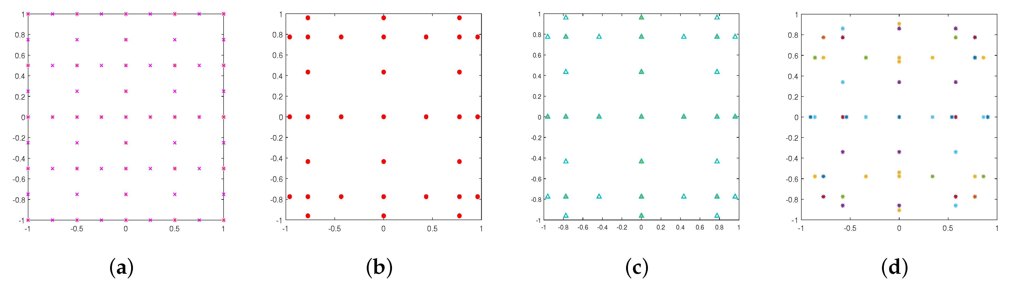
2.1. The Sparse Grid Method

We now recall the formulation of the sparse grid method for approximating (1) and its tensor product reformulation formula, which will be crucially used later in the formulation of our fast MDI-SG algorithm.

For each positive integer index $l\ge 1$, let $n_l$ be a positive integer, which denotes the number of grid points at level l and

$${\Gamma }_1^l:=\left\{x_1^l<x_2^l<\cdots <x_{n_l}^l\right\}\subset [-1,1]$$

(2)

denote a sequence of the level l grid points in $[-1,1]$. The grid set $\left\{{\Gamma }_1^l\right\}$ is said to be nested provided that ${\Gamma }_1^l\subset {\Gamma }_1^{l+1}$. The best known example of the nested grids is the following dyadic grids:

$${\Gamma }_1^l=\left\{x_i^l:=\frac{i}{2^{l-1}}:i=-2^{l-1},\cdots ,0,1,\cdots ,2^{l-1}\right\}.$$

(3)

For a given positive integer q, the tensor product $G_d^q:={\Gamma }_1^q\times {\Gamma }_1^q\times \cdots \times {\Gamma }_1^q$ then yields a standard tensor product grid on $\Omega ={[-1,1]}^d$. Notice that here the qth level is used in each coordinate direction. To reduce the number of grid points in $G_d^q$, the sparse grid idea is to restrict the total level to be q in the sense that $q=l_1+l_2+\cdots +l_d$, where $l_i$ is the level used in the ith coordinate direction. Its corresponding tensor product grid is ${\Gamma }_1^{l_1}\times {\Gamma }_1^{l_2}\times \cdots \times {\Gamma }_1^{l_d}$. Obviously, the decomposition $q=l_1+l_2+\cdots +l_d$ is not unique, so all such decomposition must be considered. The union

$${\Gamma }_d^q:=\bigcup _{l_1+\cdots +l_d=q}{\Gamma }_1^{l_1}\times \cdots \times {\Gamma }_1^{l_d}$$

(4)

then yields the famous Smolyak sparse grid (embedded) on $\Omega ={[-1,1]}^d$ (cf. [5]). We remark that the underlying idea of going from $G_d^q$ to ${\Gamma }_d^q$ is exactly the same as going from $Q_q(\Omega )$ to $P_q(\Omega )$, where $Q_q$ denotes the set of polynomials whose degrees in all coordinate directions do not exceed q and $P_q$ denotes the set of polynomials whose total degrees do not exceed q.

After having introduced the concept of sparse grids, we can then define the sparse grid quadrature rule. For a univariate function g on $[-1,1]$, we consider d, i.e., the one-dimensional quadrature formula

$${\mathcal{J}}_1^{l_i}\left(g\right):=\sum _{j=1}^{n_{l_i}}{w}_j^{l_i}g\left(x_j^{l_i}\right),i=1,\cdots ,d,$$

(5)

where $\{x_j^{l_i},j=1,\cdots ,n_{l_i}\}$ and $\{w_j^{l_i},j=1,\cdots ,n_{l_i}\}$ denote the integration points/nodes and weights of the quadrature rule, respectively, and $n_{l_i}$ denotes the number of integration points in the ith coordinate direction in $[-1,1]$. In addition, define the following:

$$\begin{array}{cc}\hfill \mathbf{l}& :=[l_1,l_2,\cdots ,l_d],\left|\mathbf{l}\right|:=l_1+l_2+\cdots +l_d,\hfill \\ \hfill {\mathcal{N}}_{d,s}& :=\left\{\mathbf{l}=[l_1,\cdots ,l_d]:\left|\mathbf{l}\right|=s,s\ge d\right\}.\hfill \end{array}$$

For example, ${\mathcal{N}}_{2,4}=\left\{[1,3],[2,2],[3,1]\right\}$.

Then, the sparse grid quadrature rule with accuracy level $q\in \mathbb{N}$ for d-dimensional integration (1) on ${[-1,1]}^d$ is defined as (cf. [1])

$$Q_d^q\left(f\right):=\sum _{q-d+1\le \left|\mathbf{l}\right|\le q}{(-1)}^{q-\left|\mathbf{l}\right|}\left(\begin{array}{c}d-1\\ q-\left|\mathbf{l}\right|\end{array}\right)\sum _{\mathbf{l}\in {\mathcal{N}}_{d,\left|\mathbf{l}\right|}}\left({\mathcal{J}}_1^{l_1}\otimes {\mathcal{J}}_1^{l_2}\otimes \cdots \otimes {\mathcal{J}}_1^{l_d}\right)f,$$

(6)

where

$$\left({\mathcal{J}}_1^{l_1}\otimes {\mathcal{J}}_1^{l_2}\otimes \cdots \otimes {\mathcal{J}}_1^{l_d}\right)f:=\sum _{j_1=1}^{n_{l_1}}\cdots \sum _{j_d=1}^{n_{l_d}}{w}_{j_1}^{l_1}\cdots w_{j_d}^{l_d}f\left(x_{j_1}^{l_1},\cdots ,x_{j_d}^{l_d}\right).$$

(7)

We note that each term $({\mathcal{J}}_1^{l_1}\otimes {\mathcal{J}}_1^{l_2}\otimes \cdots \otimes {\mathcal{J}}_1^{l_d})f$ in (7) is the tensor product quadrature rule, which uses $n_{l_i}$ integration points in the ith coordinate direction. To write $Q_d^q\left(f\right)$ more compactly, we set

$$n_d^q:=\sum _{q-d+1\le \left|\mathbf{l}\right|\le q}{n}_{l_1}\dots n_{l_d},$$

which denotes the total number of integration points in $\Omega ={[-1,1]}^d$. Let $w_k,k=1,\cdots ,n_d^q$ denote the corresponding weights and define the bijective mapping

$$\left\{{\mathbf{x}}^k:k=1,\cdots ,n_d^q\right\}⟶\left\{(x_{j_1}^{l_1},\cdots ,x_{j_d}^{l_d}):j_i=1,\cdots ,n_{l_i},q-d+1\le \left|\mathbf{l}\right|\le q\right\}.$$

Then, the sparse grid quadrature rule $Q_d^q\left(f\right)$ can be rewritten as (cf. Section 4 of [6])

$$Q_d^q\left(f\right)=\sum _{k=1}^{n_d^q}{w}_{k}f\left({\mathbf{x}}^k\right).$$

(8)

We also note that some weights $w_k$ may become negative even though the one-dimensional weights $w_{j_1}^{l_1},\cdots ,w_{j_d}^{l_d}$ are positive. Therefore, it is no longer possible to interpret $Q_d^q\left(f\right)$ as a discrete probability measure. Moreover, the existence of negative weights in (8) may cause numerical cancellation, and hence, the loss of significant digits. Circumventing such a potential cancellation, it is recommended in [6] that the summation is carried out by coordinates, this then leads to the following tensor product reformulation of $Q_d^q\left(f\right)$:

$$Q_d^q\left(f\right)=\sum _{l_1=1}^{q-1}\sum _{l_2=1}^{{\gamma }_1^q}\cdots \sum _{l_d=1}^{{\gamma }_{d-1}^q}\sum _{j_1=1}^{n_{l_1}}\cdots \sum _{j_d=1}^{n_{l_d}}{w}_{j_1}^{l_1}\cdots w_{j_d}^{l_d}f(x_{j_1}^{l_1},\cdots ,x_{j_d}^{l_d}),$$

(9)

where the upper limits are defined recursively as

$${\gamma }_0^q:=q,{\gamma }_j^q:={\gamma }_{j-1}^q-l_j,j=1,2,\cdots ,d.$$

In the nested mesh case (i.e., ${\Gamma }_1^l$ is nested), nested integration points are selected to form the sparse grid. We remark that different 1-d quadrature rules in (5) will lead to different sparse grid methods in (6). We also note that the tensor product reformulation (9) will play a crucial role later in the construction of our MD-SG algorithm.

Figure 1 demonstrates the construction of a sparse grid according to the Smolyak rule when $d=2$ and $q=4$. The meshes are nested, namely, ${\Gamma }_1^{l_i}\subset {\Gamma }_1^{l_{i+1}}$. The 1-d integration-point sequence ${\Gamma }_1^{l_1}$ ($l_1=1,2,3$, and $n_{l_1}=3,5,9$) and ${\Gamma }_1^{l_2}$ ($l_2=1,2,3$, and $n_{l_2}=3,5,9$) are shown at the top and left of the figure, and the tensor product points ${\Gamma }_1^3\otimes {\Gamma }_1^3$ are shown in the upper right corner. From (6), we see that the sparse grid rule is a combination of the low-order tensor product rule on ${\Gamma }_1^i\otimes {\Gamma }_1^j$ with $3\le i+j\le 4$. The point sets of these products and the resulting sparse grid ${\Gamma }_2^4$ are shown in the lower half of the figure. We notice that some points in the sparse grid ${\Gamma }_2^4$ are repeatedly used in ${\Gamma }_1^i\otimes {\Gamma }_1^j$ with $3\le i+j\le 4$. Consequently, we would avoid the repeated points (i.e., only using the red points in Figure 1) and use the reformulation (9), which does not involve repetition in the summation.

Figure 1. Construction of a nested sparse grid in two dimensions.

2.2. Examples of Sparse Grid Methods

As mentioned earlier, different 1-d quadrature rules in (5) lead to different sparse grid quadrature rules in (9). Below, we introduce four widely used sparse grid quadrature rules, which will be the focus of this paper.

Example 1

(The classical trapezoidal rule). The 1-d trapezoidal rule is defined by (cf. [29])

$${\mathcal{J}}_1^q\left(g\right)=\sum _{l=1}^{q-1}\sum _{j=1}^{n_l}{}^{″}{w}_j^{l}g\left(x_j^l\right)$$

(10)

with $q\ge 2$ and $n_1=1,n_l=2^{l-1}+1,w_j^l=2^{2-l},x_j^l=(j-1)·2^{2-l}-1$; where the $\sum {}^{″}$ indicates that the first and last terms in the sum are halved. The following theorem gives the error estimate; its proof can be found in [6] (pages 3–5).

Theorem 1.

Suppose $g\in {\mathcal{C}}^2:=\left\{g:\Omega \to R,\parallel \frac{{\partial }^{s}g}{\partial x^s}{\parallel }_{\infty }<\infty ,s\le 2\right\}$, then there holds

$$\left|I_1\left(g\right)-{\mathcal{J}}_1^q\left(g\right)\right|\le C{2}^{-2q}.$$

(11)

Example 2

(The classical Clenshaw-Curtis rule). This quadrature rule reads as follows (cf. [30,31]):

$${\mathcal{J}}_1^q\left(g\right)=\sum _{l=1}^{q-1}\sum _{j=1}^{n_l}{w}_j^{l}g\left(x_j^l\right)$$

(12)

with $q\ge 2,n_1=1,n_l=2^{l-1}+1,x_j^l=-cos(\pi (j-1)/(n_l-1)),j=1,\cdots ,n_l$ and the weights

$$w_1^l=w_{n_l}^l=\frac{1}{n_l(n_l-2)},w_j^l=\frac{2}{n_l-1}\left(1+2\sum _{k=1}^{\frac{n_l-1}{2}}{}^{\prime }\frac{1}{1-4k^2}cos\frac{2\pi (j-1)k}{n_l-1}\right)$$

for $2\le j\le n_l-1$; where $\sum {}^{\prime }$ indicates that the last term in the summation is halved.

The following error estimate holds and see [31] (Theorem 1) for its proof.

Theorem 2.

Suppose $g\in {\mathcal{C}}^r:=\left\{g:\Omega \to R,\parallel \frac{{\partial }^{s}g}{\partial x^s}{\parallel }_{\infty }<\infty ,s\le r\right\}$, then there holds

$$\left|I_1\left(g\right)-{\mathcal{J}}_1^q\left(g\right)\right|\le C{\left(n_1^q\right)}^{-r},where{n}_1^q:=n_1+n_2+\cdots +n_{q-1}.$$

(13)

Example 3

(The Gauss-Patterson rule). This quadrature rule is defined by (cf. [32,33])

$${\mathcal{J}}_1^q\left(g\right)=\sum _{l=1}^{q-1}\sum _{j=1}^{n_l}{w}_j^{l}g\left(x_j^l\right)$$

(14)

with $q\ge 2,n_l=2^l(n+1)-1$, and ${\left\{x_j^l\right\}}_{j=1}^{n_l}$ being the union of the zeroes of the polynomial $P_n\left(x\right)$ and $G_i\left(x\right),1\le i<l$, where $P_n\left(x\right)$ is the n-th order Legendre polynomial, $G_1\left(x\right)$ is the $(n+1)$-th order Stieltjes polynomial, and $G_i\left(x\right)$ is orthogonal to all polynomials of degree less than $2^{l-1}(n+1)$ with respect to the weight function $P_n\left(x\right)\left({\prod }_{j=1}^{i-1}{G}_j\left(x\right)\right)$. ${\left\{w_j^l\right\}}_{j=1}^{n_l}$ is defined similarly to the Gauss-Legendre case, see [32] for details. Gauss-Patterson rules are a sequence of nested quadrature formulas with the maximal order of exactness. Its error estimate is given by the following theorem, see [30,33] (Theorem 1).

Theorem 3.

Suppose $g\in {\mathcal{C}}^r:=\left\{g:\Omega \to R,\parallel \frac{{\partial }^{s}g}{\partial x^s}{\parallel }_{\infty }<\infty ,s\le r\right\}$, then there holds

$$\left|I_1\left(g\right)-{\mathcal{J}}_1^q\left(g\right)\right|\le C{\left(n_1^q\right)}^{-r},where{n}_1^q:=n_1+n_2+\cdots +n_{q-1}.$$

(15)

Example 4

(The classical Gauss-Legendre rule). This classical quadrature rule is defined by

$${\mathcal{J}}_1^q\left(g\right)=\sum _{l=1}^{q-1}\sum _{j=1}^{n_l}{w}_j^{l}g\left(x_j^l\right)$$

(16)

with $q\ge 2,n_l=l$ for $l\ge 1$. ${\left\{x_j^l\right\}}_{j=1}^{n_l}$ are the zeroes of the $n_l$th order Legendre polynomial $P_{n_l}\left(x\right)$, and ${\left\{w_j^l\right\}}_{j=1}^{n_l}$ are the corresponding weights.

The following theorem gives the error estimate; its proof can be found in [6] (pages 3–5).

Theorem 4.

Suppose $g\in {\mathcal{C}}^r:=\left\{g:\Omega \to R,\parallel \frac{{\partial }^{s}g}{\partial x^s}{\parallel }_{\infty }<\infty ,s\le r\right\}$, then there holds

$$\left|I_1\left(g\right)-{\mathcal{J}}_1^q\left(g\right)\right|\le C{\left(n_1^q\right)}^{-r},where{n}_1^q:=n_1+n_2+\cdots +n_{q-1}.$$

(17)

Figure 2 and Figure 3 show the resulting sparse grids of the above four examples in both 2-d and 3-d cases with $q=6$ and $q=7$, respectively. We note that these four sparse grids have different structures.

Figure 2. Sparse grids corresponding to the trapezoidal rule (a), Clenshaw-Curtis rule (b), Gauss-Patterson rule (c), and Gauss-Legendre rule (d) when $d=2,q=6$.

Figure 3. Sparse grids corresponding to the trapezoidal rule (a), Clenshaw-Curtis rule (b), Gauss-Patterson rule (c), and Gauss-Legendre rule (d) when $d=3,q=7$.

We conclude this section by remarking that the error estimates of the above quadrature rules can be easily translated to error estimates for the sparse grid method (9). For example, in the case of the Clenshaw-Curtis, Gauss-Patterson, and Gauss-Legendre quadrature rule, there holds (cf. [31] (Corollary 1))

$$\left|I_d\left(f\right)-Q_d^q\left(f\right)\right|\le C{\left(n_d^q\right)}^{-r}·{\left(\log \left(n_d^q\right)\right)}^{(d-1)(r+1)}\forall f\in W_d^r,$$

(18)

where

$$n_d^q:=\sum _{q-d+1\le \left|\mathbf{l}\right|\le q}{n}_{l_1}\dots n_{l_d},$$

$$W_d^r:=\{f:\Omega \to \mathbb{R};|\frac{{\partial }^{\left|\mathbf{l}\right|}f}{\partial x_1^{l_1}\cdots \partial x_d^{l_d}}|{}_{\infty }<\infty ,l_i\le r,i=1,2,\cdots ,d\}.$$

We note that the above estimate indicates that the error of the sparse grid method still deteriorates exponentially in the dimension d, but with a smaller base $log\left(n_d^q\right)$.

3. The MDI-SG Algorithm

The goal of this section is to present an efficient and fast implementation algorithm (or solver), called the MDI-SG algorithm, for evaluating the sparse grid quadrature rule (6) via its reformulation (9) in order to circumvent the curse of dimensionality, which hampers the usage of the sparse grid method (6) in high dimensions. To better understand the main idea of the MDI-SG method, we first consider the simple two- and three-dimensional cases and then formulate the algorithm in arbitrary dimensions.

Recall that $f\left(\mathbf{x}\right):\overline{\Omega }$$\to R$ denotes a continuous function on $\overline{\Omega }\subset {\mathbb{R}}^d$; we assume that f has a known expression.

3.1. Formulation of the MDI-SG Algorithm in Two Dimensions

Let $d=2$, $\Omega ={[-1,1]}^2$, and $\mathbf{x}=(x_1,x_2)\in \Omega$. Using Fubini’s theorem, we have

$$I_2\left(f\right):={\int }_{{[-1,1]}^2}f\left(\mathbf{x}\right)d\mathbf{x}={\int }_{-1}^1\left({\int }_{-1}^{1}f(x_1,x_2)d{x}_1\right)d{x}_2.$$

(19)

Then, the two-dimensional SG quadrature rule (9) takes the form

$$Q_2^q\left(f\right)=\sum _{l_1=1}^{q-1}\sum _{l_2=1}^{{\gamma }_1^q}\sum _{j_1=1}^{n_{l_1}}\sum _{j_2=1}^{n_{l_2}}{w}_{j_1}^{l_1}{w}_{j_2}^{l_2}f(x_{j_1}^{l_1},x_{j_2}^{l_2}),$$

(20)

where ${\gamma }_1^q=q-l_1$. Motivated by (and mimicking) Fubini’s Formula (19), we rewrite (20) as

$$\begin{array}{cc}\hfill Q_2^q\left(f\right)& =\sum _{l_2=1}^{{\gamma }_1^q}\sum _{j_2=1}^{n_{l_2}}{w}_{j_2}^{l_2}\left(\sum _{l_1=1}^{q-1}\sum _{j_1=1}^{n_{l_1}}{w}_{j_1}^{l_1}f(x_{j_1}^{l_1},x_{j_2}^{l_2})\right)\hfill \\ \hfill & =\sum _{l_2=1}^{{\gamma }_1^q}\sum _{j_2=1}^{n_{l_2}}{w}_{j_2}^{l_2}{f}_1\left(x_{j_2}^{l_2}\right),\hfill \end{array}$$

(21)

where

$$f_1\left(s\right):=\sum _{l_1=1}^{q-1}\sum _{i=1}^{n_{l_1}}{w}_i^{l_1}f(x_i^{l_1},s).$$

We note that the evaluation of $f_1\left(x_2\right)$ amounts to applying the 1-d Formula (5) to approximate the integral ${\int }_{-1}^{1}f(x_1,x_2)d{x}_1.$ However, the values of $\left\{f_1\left(x_{j_2}^{l_2}\right)\right\}$ will not be computed by the 1-d quadrature rule in our MDI-SG algorithm; instead, $f_1$ is formed as a symbolic function, so the 1-d quadrature rule can be called on $f_1$. Therefore, we still use the SG method to select the integration points, and then use our MDI-SG algorithm to perform function evaluations at the integration points collectively to save computation, which is the main idea of the MDI-SG method.

Let W and X denote the weight and node vectors of the 1-d quadrature rule on $[-1,1]$. In addition, $n_{l_i}$ represents the number of integration points in the $x_i$ direction and we use a parameter $r\in \{1,2,3,4\}$ to indicate one of the four quadrature rule. The following algorithm implements the sparse grid quadrature Formula (21).

We note that the first do-loop forms the symbolic function $f_1$, which encodes all computations involving the $x_1$-components at all integration points. The second do-loop evaluates the 1-d quadrature rule for the function $f_1$. As mentioned above, in this paper, we only focus on the four well-known 1-d quadrature rules: (i) the trapezoidal rule; (ii) the Clenshaw-Curtis rule; (iii) the Gauss-Patterson rule; (iv) the Gauss-Legendre rule. They will be represented respectively by $r=1,2,3,4$.

Below, we use a simple 2-d example to explain the mechanism of above 2d-MDI-SG algorithm. It is clear that to directly compute the SD sum

$$\sum _{i_1=1}^{n_1}\sum _{i_2=1}^{n_2}f({\xi }_{i_1},{\xi }_{i_2})=f({\xi }_1,{\xi }_1)+f({\xi }_1,{\xi }_2)+\cdots +f({\xi }_{n_1},{\xi }_{n_2}),$$

(22)

it is necessary to compute the function values of $f(x_1,x_2)$ at $n_1{n}_2$ points, which is often performed independently. On the other hand, the 2d-MDI-SD algorithm is based on rewriting the sum as

$$\sum _{i_1=1}^{n_1}\sum _{i_2=1}^{n_2}f({\xi }_{i_1},{\xi }_{i_2})=\sum _{i_1=1}^{n_1}{f}_1\left({\xi }_{i_1}\right),$$

(23)

where $f_1\left(x_1\right)={\sum }_{i_2}^{n_2}f(x_1,{\xi }_{i_2})$ denotes the symbolic function obtained in the first do-loop. Hence, the algorithm performs two separate do-loops. In the first d-loop, symbolic computations are performed to obtain the symbolic function $f_1\left(x_1\right)$, which is saved. In the second do-loop, the single sum ${\sum }_{i_1=1}^{n_1}{f}_1\left({\xi }_{i_1}\right)$ is calculated. When computing the symbolic function $f_1\left(x_1\right)$, a lot of computations have been reused for computing the coefficients in $f_1\left(x_1\right)$, and those coefficients are constants in the second do-loop. Efficiently generating the symbolic function and using it to compute the SG sum are the main reasons for saving computation and computer memory.

Take $f(x_1,x_2)=x_1^2+x_1{x}_2+x_2^2$ as a concrete example. The direct computation the SG sum in (22) requires to compute the function value $f({\xi }_1,{\xi }_2)={\xi }_1^2+{\xi }_1{\xi }_2+{\xi }_2^2$ at each node $({\xi }_1,{\xi }_2)$; this, in turn, requires three multiplications and two additions. With a total of $n_1{n}_2$ nodes, the computing the sum requires a total of $3n_1{n}_2$ multiplications and $3n_1{n}_2-1$ additions. On the other hand, when using the 2d-MDI-SD algorithm to compute the same sum, in the first do-loop, we compute the symbolic function $f_1\left(x_1\right)={\sum }_{i_2=1}^{n_2}f(x_1,{\xi }_{i_2})$, which requires $n_2$ “symbolic multiplications” of ${\xi }_{i_2}{x}_1$ (no real multiplication is needed because of its linear dependence on ${\xi }_{u_2}$ and $n_2$ multiplications of ${\xi }_{i_2}^2$, and $3n_2-1$ additions. In the second do-loop, computing the ${\sum }_{i_1=1}^{n_1}{f}_1\left({\xi }_{i_1}\right)$ requires $n_1$ multiplications of ${\xi }_{i_1}^2$ and $n_1$ multiplications of ${\xi }_{i_1}{\overline{\xi }}_{i_2}$, and $3n_1-1$ additions. Thus, the 2d-MDI-SD algorithm requires a total of $2(n_1+n_2)$ multiplications and $3(n_1+n_2-\frac{4}{3})$ additions. Therefore, the 2d-MDI-SG algorithm computes the SD sum much more economically than the standard implementation, and this advantage will become more significant in high dimensions. See Section 3.2 and Section 3.3 for details.

3.2. Formulation of the MDI-SG Algorithm in Three Dimensions

In the subsection, we extend the formulation of the above 2d-MDI-SGI algorithm to the 3-d case by highlighting its main steps, in particular, how the above 2-d algorithm is utilized. First, recall that Fubini’s theorem is given by

$$I_3\left(f\right):={\int }_{{[-1,1]}^3}f\left(\mathbf{x}\right)d\mathbf{x}={\int }_{{[-1,1]}^2}\left({\int }_{-1}^{1}f\left(\mathbf{x}\right)d{x}_1\right)d{\mathbf{x}}^{\prime },$$

(24)

where ${\mathbf{x}}^{\prime }=(x_2,x_3)$.

Second, notice that the SG quadrature rule (9) in 3-d takes the form

$$Q_3^q\left(f\right)=\sum _{l_1=1}^{q-1}\sum _{l_2=1}^{{\gamma }_1^q}\sum _{l_3=1}^{{\gamma }_2^q}\sum _{j_1=1}^{n_{l_1}}\sum _{j_2=1}^{n_{l_2}}\sum _{j_3=1}^{n_{l_3}}{w}_{j_1}^{l_1}{w}_{j_2}^{l_2}{w}_{j_3}^{l_3}f(x_{j_1}^{l_1},x_{j_2}^{l_2},x_{j_3}^{l_3}).$$

(25)

where ${\gamma }_2^q=q-l_1-l_2$. Mimicking Fubini’s formula above, we rewrite (25) as

$$\begin{array}{cc}\hfill Q_3^q\left(f\right)& =\sum _{l_3=1}^{{\gamma }_2^q}\sum _{j_3=1}^{n_{l_3}}\sum _{l_2=1}^{{\gamma }_1^q}\sum _{j_2=1}^{n_{l_2}}{w}_{j_3}^{l_3}{w}_{j_2}^{l_2}\left(\sum _{l_1=1}^{q-1}\sum _{j_1=1}^{n_{l_1}}{w}_{j_1}^{l_1}f(x_{j_1}^{l_1},x_{j_2}^{l_2},x_{j_3}^{l_3})\right)\hfill \\ \hfill & =\sum _{l_3=1}^{{\gamma }_2^q}\sum _{j_3=1}^{n_{l_3}}\sum _{l_2=1}^{{\gamma }_1^q}\sum _{j_2=1}^{n_{l_2}}{w}_{j_3}^{l_3}{w}_{j_2}^{l_2}{f}_2(x_{j_2}^{l_2},x_{j_3}^{l_3}),\hfill \end{array}$$

(26)

where

$$f_2(s,t):=\sum _{l_1=1}^{q-1}\sum _{j_1=1}^{n_{l_1}}{w}_{j_1}^{l_1}f(x_{j_1}^{l_1},s,t).$$

(27)

We note that $f_2$ is formed as a symbolic function in our MDI-SG algorithm and the right-hand side of (26) is viewed as a 2-d sparse grid quadrature formula for $f_2$; it can be computed either directly or recursively by using Algorithm 1. The following algorithm implements the SG quadrature Formula (26).

Algorithm 1: 2d-MDI-SG (f, $\Omega ,r,q,X,W$)

Initialize $Q=0$, $f_1=0$. for $l_1=1:q$ do      for $j_1=1:n_{l_1}$ do         $f_1=f_1+W_{j_1}^{l_1}f\left((X_{j_1}^{l_1},·)\right)$.      end for end for for $l_2=1:q-l_1$ do      for $j_2=1:n_{l_2}$ do         $Q=Q+W_{j_2}^{l_2}·f_1\left(X_{j_2}^{l_2}\right)$.      end for end for return Q.

Where $P_3^2$ denotes the orthogonal projection (or natural embedding): $x=(x_1,x_2,x_3)$$\to {\mathbf{x}}^{\prime }=(x_2,x_3)$, and W and X stand for the weight and node vectors of the underlying 1-d quadrature rule, respectively.

From Algorithm 2 we can see the mechanism of the MDI-SG algorithm. It is based on two main ideas: (i) Using the sparse grid approach to select integration points; (ii) using the discrete Fubini formula to efficiently compute the total sparse grid sum by reducing it to the calculation of a low-dimensional (i.e., 2-d) sparse grid sum, which allows us to recursively call the low-dimensional MDI-SG algorithm.

Algorithm 2: 3d-MDI-SG(f, $\Omega ,r,q,X,W$)

Initialize $Q=0,f_2=0$. for $l_1=1:q$ do      for $j_1=1:n_{l_1}$ do         $f_2=f_2+W_{j_1}^{l_1}·f\left((X_{j_1}^{l_1},·,·)\right)$.      end for end for ${\Omega }_2=P_3^2\Omega ,{\gamma }_1^q=q-l_1$. $Q=$2d-MDI-SG$(f_2,{\Omega }_2,r,{\gamma }_1^q,X,W)$. return Q.

3.3. Formulation of the MDI-SG Algorithm in Arbitrary d-Dimensions

The goal of this subsection is to extend the 2-d and 3-d MDI-SG algorithms to arbitrary d-dimensions. We again start by recalling the d-dimensional Fubini’s theorem

$$I_d\left(f\right)={\int }_{\Omega }f\left(\mathbf{x}\right)d\mathbf{x}={\int }_{{\Omega }_{d-m}}\left({\int }_{{\Omega }_m}f\left(\mathbf{x}\right)d{\mathbf{x}}^{\prime \prime }\right)d{\mathbf{x}}^{\prime },$$

(28)

where $1\le m<d$, $\Omega ={[-1,1]}^d,{\Omega }_m={\rho }_d^m\Omega ={[-1,1]}^m$ and ${\Omega }_{d-m}=P_d^{d-m}\Omega ={[-1,1]}^{d-m}$ in which ${\rho }_d^m$ and $P_d^{d-m}$ denote the orthogonal projections (or natural embeddings): $\mathbf{x}=(x_1,x_2,\cdots ,x_d)\to {\mathbf{x}}^{\prime \prime }=(x_1,x_2,\cdots ,x_m)$ and $\mathbf{x}=(x_1,x_2,\cdots ,x_d)\to {\mathbf{x}}^{\prime }=(x_{m+1},x_{m+2},\cdots ,x_d)$, respectively. The integer m denotes the dimension reduction step length in our algorithm.

Mimicking Fubini’s theorem above, we rewrite the d-dimensional SG quadrature rule (9) as follows:

$$\begin{array}{cc}\hfill Q_d^q\left(f\right)& =\sum _{l_d=1}^{{\gamma }_{d-1}^q}\sum _{j_d=1}^{n_{l_d}}\cdots \sum _{l_{m+1}=1}^{{\gamma }_m^q}\sum _{j_{m+1}}^{n_{l_{m+1}}}{w}_{j_{m+1}}^{l_{m+1}}\cdots w_{j_d}^{l_d}\left(\sum _{l_m=1}^{{\gamma }_{m-1}^q}\cdots \sum _{j_1=1}^{n_{l_1}}{w}_{j_1}^{l_1}\cdots w_{j_m}^{l_m}f(x_{j_1}^{l_1},\cdots ,x_{j_d}^{l_d})\right)\hfill \\ \hfill & =\sum _{l_d=1}^{{\gamma }_{d-1}^q}\sum _{j_d=1}^{n_{l_d}}\cdots \sum _{l_{m+1}=1}^{{\gamma }_m^q}\sum _{j_{m+1}=1}^{n_{l_{m+1}}}{w}_{j_{m+1}}^{l_{m+1}}\cdots w_{j_d}^{l_d}{f}_{d-m}(x_{j_{m+1}}^{l_{m+1}},\cdots ,x_{j_d}^{l_d}),\hfill \end{array}$$

(29)

where

$$\begin{array}{c}\hfill f_{d-m}(s_1,\cdots ,s_{d-m})=\sum _{l_m=1}^{{\gamma }_{m-1}^q}\sum _{j_m=1}^{n_{l_m}}\cdots \sum _{l_1=1}^{q-1}\sum _{j_1=1}^{n_{l_1}}{w}_{j_1}^{l_1}\cdots w_{j_m}^{l_m}f(x_{j_1}^{l_1},\cdots ,x_{j_m}^{l_m},s_1,\cdots ,s_{d-m}).\end{array}$$

(30)

We note that, in our MDI-SG algorithm, $f_{d-m}$ defined by (30) is a symbolic function and the right-hand side of (29) is a $(d-m)$-order multisummation, which itself can be evaluated by employing the dimension reduction strategy. Dimensionality can be reduced by iterating $k:=\left[\frac{d}{m}\right]$ times until $d-km\le m$. To implement this process, we introduce the following conventions:

• If $t=1$, set MDI-SG$(t,f_t,{\Omega }_t,m,s,r,q,X,W):={\mathcal{J}}_1^q\left(f\right)$, which is computed by using the one-dimensional quadrature rule (5);
• If $t=2$, set MDI-SG$(t,f_t,{\Omega }_t,m,s,r,q,X,W):=$ 2d-MDI-SG$(f_t,{\Omega }_t,r,q,X,W)$;
• If $t=3$, set MDI-SG$(t,f_t,{\Omega }_t,m,s,r,q,X,W):=$ 3d-MDI-SG$(f_t,{\Omega }_t,r,q,X,W)$.

We note that when $t=1,2,3$, the parameter m becomes a dummy variable and can be given any value. Recall that $P_t^{t-m}$ denotes the natural embedding from ${\mathbb{R}}^t$ to ${\mathbb{R}}^{t-m}$ by deleting the first m components of vectors in ${\mathbb{R}}^t$. The following algorithm implements the sparse grid quadrature via (29) with

$$\begin{array}{c}\hfill f_{t-m}(s_1,\cdots ,s_{t-m})=\sum _{l_m=1}^{{\gamma }_{m-1}^q}\sum _{j_m=1}^{n_{l_m}}\cdots \sum _{l_1=1}^{q-1}\sum _{j_1=1}^{n_{l_1}}{w}_{j_1}^{l_1}\cdots w_{j_m}^{l_m}·f(x_{j_1}^{l_1},\cdots ,x_{j_m}^{l_m},s_1^{},\cdots ,s_{t-m}).\end{array}$$

(31)

Algorithm 3 recursively generates a sequence of symbolic functions $f_d,\cdots ,f_{d-km},$$f_{d-km-s},\cdots ,f_{d-km-k_{1}s}$; each function has m fewer arguments than its predecessor. As mentioned earlier, our MDI-SG algorithm does not perform the function evaluations at all integration points independently, but rather iteratively along m-coordinate directions; hence, the function evaluation at any integration point is not completed until the last step of the algorithm is executed. As a result, many computations are reused in each iteration, which is the main reason for the computational savings and achieving a faster algorithm.

Algorithm 3: MDI-SG$(d,f,\Omega ,m,s,r,q,X,W)$

${\Omega }_d=\Omega ,f_d=f,k=\left[\frac{d}{m}\right],{\gamma }_d^q=q-1$. for $t=d:-m:d-km$ (the index is decreased by m at each iteration) do     ${\Omega }_{d-m}=P_t^{t-m}{\Omega }_t,{\gamma }_{d-m}^q={\gamma }_t^q-l_1-\cdots -l_m$.     (Construct symbolic function $f_{t-m}$ by (31) below).     $\mathrm{MDI}-\mathrm{SG}(t,f_t,{\Omega }_t,m,s,r,{\gamma }_t^q,X,W):=\mathrm{MDI}-\mathrm{SG}(t-m,f_{t-m},{\Omega }_{t-m},m,s,r,{\gamma }_{t-m}^q,X,W)$ end for $d=d-km,s=1(\mathrm{or} 2,3),f_d=f_t,k_1=\left[\frac{d-km}{s}\right]$. for $t=d:-s:d-k_{1}s$ (the index is decreased by s at each iteration) do     ${\Omega }_{d-s}=P_t^{t-s}{\Omega }_t,{\gamma }_{d-s}^q={\gamma }_t^q-l_1-\cdots -l_s$.     (Construct symbolic function $f_{t-s}$ by (31) below).     $\mathrm{MDI}-\mathrm{SG}(t,f_t,{\Omega }_t,m,s,r,{\gamma }_t^q,X,W):=\mathrm{MDI}-\mathrm{SG}(t-s,f_{t-s},{\Omega }_{t-s},m,s,r,{\gamma }_{t-s}^q,X,W)$ end for $Q=\mathrm{MDI}-\mathrm{SG}(d-k_{1}s,f_{d-k_{1}s},{\Omega }_{d-k_{1}s},m,s,r,{\gamma }_{d-k_{1}s}^q,X,W).$ returnQ.

Remark 1.

We note that as a solver-type algorithm, the proposed MDI-SG algorithm provides an efficient and fast way to implement the widely used sparse grid methods reviewed in Section 2.2; it does not improve or reduce the theoretical convergence rate of the underlying sparse grid method. As a result, the numerical results obtained by our MDI-SG algorithm also obey the same theoretical error bounds stated in Theorems 1–4 depending on the choice of the underlying sparse grid method.

4. Numerical Performance Tests

In this section, we present extensive numerical tests to gauge the performance of the proposed MDI-SG algorithm and to compare it with the standard sparse grid (SG) and classical Monte Carlo (MC) methods. All numerical tests show that MDI-SG algorithm outperforms both the SG and MC methods in low and medium/high dimensions (i.e., $d\lesssim 100$), and can compute very high-dimensional (i.e., $d\approx 1000$) integrals while others fail.

All our numerical experiments were performed in Matlab 9.4.0.813654(R2018a) on a desktop PC with Intel(R) Xeon(R) Gold 6226R CPU 2.90GHz and 32GB RAM.

4.1. Two- and Three-Dimensional Tests

We first tested our MDI-SG algorithm on simple 2-d and 3-d examples and compared its performance (in terms of CPU time) with the SG methods.

Test 1. Let $\Omega ={[-1,1]}^2$ and consider the following 2-d integrands:

$$f\left(x\right):=exp\left(5x_1^2+5x_2^2\right);\widehat{f}\left(x\right):=sin\left(2\pi +10x_1^2+5x_2^2\right).$$

(32)

Let q denote the accuracy level of the sparse grid. The larger q is, the more integration points we need for the 1-d quadrature rule, and the higher the accuracy of the MDI-SG quadrature. The base 1-d quadrature rule was chosen to be the Gauss-Patterson rule; hence, parameter $r=3$ in the algorithm.

Table 1 and Table 2 present the computational results (errors and CPU times) of the MDI-SG and SG methods for approximating $I_2\left(f\right)$ and $I_2\left(\widehat{f}\right)$, respectively.

Table 1. Relative errors and CPU times of MDI-SG and SG tests with $m=1$ for approximating $I_2\left(f\right)$.

		MDI-SG		SG
Accuracy Level $\left(\mathit{q}\right)$	Total Nodes	Relative Error	CPU Time (s)	Relative Error	CPU Time (s)
6	33	$1.0349\times {10}^{-1}$	0.0512817	$1.0349\times {10}^{-1}$	0.0078077
7	65	$2.3503\times {10}^{-3}$	0.0623538	$2.3503\times {10}^{-3}$	0.0084645
9	97	$8.1019\times {10}^{-4}$	0.0644339	$8.1019\times {10}^{-4}$	0.0095105
10	161	$1.8229\times {10}^{-6}$	0.0724491	$1.8229\times {10}^{-6}$	0.0106986
13	257	$2.0720\times {10}^{-7}$	0.0913161	$2.0720\times {10}^{-7}$	0.0135131
14	321	$4.3279\times {10}^{-7}$	0.1072016	$4.3279\times {10}^{-7}$	0.0155733

Table 2. Relative errors and CPU times of MDI-SG and SG tests with $m=1$ for approximating $I_2(\widehat{f}$).

		MDI-SG		SG
Accuracy Level $\left(\mathit{q}\right)$	Total Nodes	Relative Error	CPU Time (s)	Relative Error	CPU Time (s)
9	97	$4.7425\times {10}^{-1}$	0.0767906	$4.7425\times {10}^{-1}$	0.0098862
10	161	$1.4459\times {10}^{-3}$	0.0901238	$1.4459\times {10}^{-3}$	0.0102700
13	257	$1.9041\times {10}^{-5}$	0.1025934	$1.9041\times {10}^{-5}$	0.0152676
14	321	$2.3077\times {10}^{-5}$	0.1186194	$2.3077\times {10}^{-5}$	0.0144737
16	449	$3.1236\times {10}^{-6}$	0.1353691	$3.1236\times {10}^{-6}$	0.0177445
20	705	$2.4487\times {10}^{-6}$	0.1880289	$2.4487\times {10}^{-6}$	0.0355606

From Table 1 and Table 2, we can see that these two methods used very little CPU time; however, despite the SG method outperforming the MDI-SG method in both tests, the difference was almost negligible, so both methods performed well in 2-d case.

Test 2. Let $\Omega ={[-1,1]}^3$ and we consider the following 3-d integrands:

$$f\left(x\right)=exp\left(5x_1^2+5x_2^2+5x_3^2\right),\widehat{f}\left(x\right)=sin\left(2\pi +10x_1^2+5x_2^2+5x_3\right).$$

(33)

We computed the integral of these two functions over $\Omega ={[-1,1]}^3$ using the MDI-SG and SG methods. Similarly, let q denote the accuracy level of the sparse grid. In addition, we chose parameters $r=3$ and $m=1$ in the algorithm.

The test results are given in Table 3 and Table 4. We again can see that both methods used very little CPU time; although the SG method again slightly outperformed the other method in both tests. However, as q increased, the number of integration points increased, and the CPU times used by these two methods became closer. We would like to point out that both methods were very efficient and their difference was negligible in the 3-d case.

Table 3. Relative errors and CPU times of MDI-SG and SG tests with $m=1$ for approximating $I_3\left(f\right)$.

		MDI-SG		SG
Accuracy Level $\left(\mathit{q}\right)$	Total Nodes	Relative Error	CPU Time (s)	Relative Error	CPU Time (s)
9	495	$3.2467\times {10}^{-2}$	0.0669318	$3.2467\times {10}^{-2}$	0.0235407
10	751	$1.8956\times {10}^{-3}$	0.0886774	$1.8956\times {10}^{-3}$	0.0411750
11	1135	$3.9146\times {10}^{-4}$	0.0902602	$3.9146\times {10}^{-4}$	0.0672375
13	1759	$4.7942\times {10}^{-6}$	0.1088353	$4.7942\times {10}^{-6}$	0.0589584
14	2335	$1.8013\times {10}^{-6}$	0.1381728	$1.8013\times {10}^{-6}$	0.0704032
15	2527	$1.2086\times {10}^{-6}$	0.1484829	$1.2086\times {10}^{-6}$	0.0902680
16	3679	$3.6938\times {10}^{-7}$	0.1525743	$3.6938\times {10}^{-7}$	0.1143728

Table 4. Relative errors and CPU times of MDI-SG and SG tests with $m=1$ for approximating $I_3\left(\widehat{f}\right)$.

		MDI-SG		SG
Accuracy Level $\left(\mathit{q}\right)$	Total Nodes	Relative Error	CPU Time (s)	Relative Error	CPU Time (s)
12	1135	$5.5057\times {10}^{-1}$	0.0921728	$5.5057\times {10}^{-1}$	0.0495310
13	1759	$8.9519\times {10}^{-3}$	0.1031632	$8.9519\times {10}^{-3}$	0.0644124
15	2527	$1.8063\times {10}^{-3}$	0.1771094	$1.8063\times {10}^{-3}$	0.0891040
16	3679	$1.1654\times {10}^{-4}$	0.1957219	$1.1654\times {10}^{-4}$	0.1159222
17	4447	$2.4311\times {10}^{-5}$	0.2053174	$2.4311\times {10}^{-5}$	0.1443184
19	6495	$5.4849\times {10}^{-6}$	0.4801467	$5.4849\times {10}^{-6}$	0.2259950
20	8031	$1.5333\times {10}^{-6}$	0.6777698	$1.5333\times {10}^{-6}$	0.2632516

4.2. High-Dimensional Tests

In this section, we evaluate the performance of the MDI-SG method for $d>>1$. First, we tested and compared the performance of the MDI-SG and SG methods in computing Gaussian integrals for dimensions $2\le d\le 20$ because $d\approx 20$ is the highest dimension that the SG method is able to compute on our computer. We then provide a performance comparison (in terms of CPU time) of the MDI-SG and classical Monte Carlo (MC) methods in computing high-dimensional integrals.

Test 3. Let $\Omega ={[-1,1]}^d$ for $2\le d\le 20$ and consider the following Gaussian integrand:

$$f\left(\mathbf{x}\right)=\frac{1}{\sqrt{2\pi }}exp\left(-\frac{1}{2}{\left|\mathbf{x}\right|}^2\right),$$

(34)

where $\left|\mathbf{x}\right|$ stands for the Euclidean norm of the vector $\mathbf{x}\in {\mathbb{R}}^d$.

We computed the integral $I_d\left(f\right)$ by using the MDI-SG and SG methods, as was done in Tests 1 and 2. Both methods were based on the same 1-d Gauss-Patterson rule (i.e., the parameter $r=3$). We also set $m=1,s=1$ in the MDI-SG method and used two accuracy levels: $q=10,12$.

Table 5 gives the relative error and CPU time for approximating $I_d\left(f\right)$ using the MDI-SG and SG methods with the accuracy level $q=10$, and Table 6 gives the corresponding results for $q=12$. As can be observed, the errors were the same for both methods (since they used the same integration points), but their CPU times were quite different. The SG method was more efficient for $d\le 4$ when $q=8,10$ and for $d\le 3$ when $q=12$, but the MDI-SG method excelled for $d\ge 4$ and the winning margin became significant as d and q increased (also see Figure 4). For example, when $d=14$ and $q=10$, the CPU time required by the SG method was about 6167 s, which is about 2 h, but the CPU time of the MDI-SG method was less than 1 s. Also, when $d=13$ and $q=12$, the SG method failed to compute the integral due to running out of computer memory. This is because the large number of integration points need to be saved and function evaluations must be performed. The MDI-SG method only needed about 2 s to complete the computation.

Table 5. Relative errors and CPU times of MDI-SG and SG tests with $m=1,s=1$, and $q=10$ for approximating $I_d\left(f\right)$.

		MDI-SG		SG
Dimension ($\mathit{d}$)	Total Nodes	Relative Error	CPU Time (s)	Relative Error	CPU Time (s)
2	161	$1.0163\times {10}^{-8}$	0.0393572	$1.0163\times {10}^{-8}$	0.0103062
4	2881	$2.0310\times {10}^{-8}$	0.0807326	$2.0310\times {10}^{-8}$	0.0993984
8	206465	$1.3429\times {10}^{-7}$	0.1713308	$1.3429\times {10}^{-7}$	6.7454179
10	1041185	$1.6855\times {10}^{-6}$	0.2553576	$1.6855\times {10}^{-6}$	86.816883
12	4286913	$1.8074\times {10}^{-5}$	0.3452745	$1.8074\times {10}^{-5}$	866.1886366
14	5036449	$2.1338\times {10}^{-4}$	0.4625503	$2.1338\times {10}^{-4}$	6167.3838002
15	12533167	$7.1277\times {10}^{-4}$	0.5867914	failed	failed

Table 6. Relative errors and CPU times of MDI-SG and SG tests with $m=1,s=1$, and $q=12$ for approximating $I_d\left(f\right)$.

		MDI-SG		SG
Dimension ($\mathit{d}$)	Total Nodes	Relative Error	CPU Time (s)	Relative Error	CPU Time (s)
2	161	$1.0198\times {10}^{-8}$	0.0418615	$1.0198\times {10}^{-8}$	0.0191817
4	6465	$2.0326\times {10}^{-8}$	0.0704915	$2.0326\times {10}^{-8}$	0.2067346
6	93665	$3.0487\times {10}^{-8}$	0.0963325	$3.0487\times {10}^{-8}$	3.1216913
8	791169	$4.0881\times {10}^{-8}$	0.2233707	$4.0881\times {10}^{-8}$	41.3632962
10	5020449	$4.0931\times {10}^{-8}$	0.3740873	$4.0931\times {10}^{-8}$	821.6461622
12	25549761	$1.1560\times {10}^{-6}$	0.8169479	$1.1560\times {10}^{-6}$	11,887.797686
13	29344150	$5.2113\times {10}^{-6}$	1.2380811	failed	failed

Figure 4. CPU time comparison of MDI-SG and SG tests: $q=8$ (left); $q=10$ (middle); $q=12$ (right).

The classical (and quasi) Monte Carlo (MC) method is often the preferred/default method for computing high-dimensional integrals. However, due to its low order of convergence, to achieve the accuracy, a large number of function evaluations are required at randomly sampled integration points, and the number grows rapidly as dimension d increases (due to the rapid growth of variance). Below, we compare the performance of the MDI-SG (with parameters $r=3,q=10,m=10,s=1$) and classical MC method. In the test, when $d\ge 10$, we used the iteration step length $m>1$ to iterate faster until $d-km\le m$ to reach stage 2 of the iteration. We refer the reader to Section 5.2 for a detailed analysis.

Test 4. Let $\Omega ={[-1,1]}^d$ and choose the following integrands:

$$f\left(x\right)=\prod _{i=0}^d\frac{1}{0.9^2+{(x_i-0.6)}^2},\widehat{f}\left(x\right)=\frac{1}{\sqrt{2\pi }}exp\left(-\frac{1}{2}{\left|x\right|}^2\right).$$

(35)

We used relative error as a criterion for comparison, that is, we determined a required (minimum) number of random sampling points for the MC method so that it produced a relative error comparable to that of the MDI-SG method. The computed results for $I_d\left(f\right)$ and $I_d\left(\widehat{f}\right)$ are given in Table 7 and Table 8, respectively.

Table 7. CPU times of the MDI-SG and MC tests with comparable relative errors for approximating $I_d\left(f\right)$.

	MC		MDI-SG
Dimension ($\mathit{d}$)	Relative Error	CPU Time (s)	Relative Error	CPU Time (s)
5	$1.3653\times {10}^{-5}$	62.1586394	$1.3653\times {10}^{-5}$	0.0938295
10	$2.0938\times {10}^{-5}$	514.1493073	$2.0938\times {10}^{-5}$	0.1945813
20	$4.2683\times {10}^{-5}$	1851.0461899	$4.1876\times {10}^{-5}$	0.4204564
30	$6.2814\times {10}^{-5}$	15,346.222011	$6.2814\times {10}^{-5}$	0.7692118
35	$7.3283\times {10}^{-5}$	failed	$7.3283\times {10}^{-5}$	0.9785784
40	$8.3752\times {10}^{-5}$		$8.3752\times {10}^{-5}$	1.2452577
60	$1.2562\times {10}^{-4}$		$1.2562\times {10}^{-4}$	2.5959174
80	$1.6750\times {10}^{-4}$		$1.6750\times {10}^{-4}$	4.9092032
100	$2.1235\times {10}^{-4}$		$2.1235\times {10}^{-4}$	8.1920274

Table 8. CPU times of the MDI-SG and MC tests with comparable relative errors for approximating $I_d\left(\widehat{f}\right)$.

	MC		MDI-SG
Dimension ($\mathit{d}$)	Relative Error	CPU Time (s)	Relative Error	CPU Time (s)
5	$9.4279\times {10}^{-7}$	85.2726354	$9.4279\times {10}^{-7}$	0.0811157
10	$1.6855\times {10}^{-6}$	978.1462121	$1.6855\times {10}^{-6}$	0.295855
20	$3.3711\times {10}^{-6}$	2038.138555	$3.3711\times {10}^{-6}$	6.3939110
30	$5.0567\times {10}^{-6}$	16,872.143255	$5.0567\times {10}^{-6}$	29.5098187
35	$5.8995\times {10}^{-6}$	failed	$5.8995\times {10}^{-6}$	62.0270714
40	$6.7423\times {10}^{-6}$		$6.7423\times {10}^{-6}$	106.1616486
80	$1.3484\times {10}^{-5}$		$1.3484\times {10}^{-5}$	1893.8402620
100	$1.7825\times {10}^{-5}$		$1.7825\times {10}^{-5}$	3077.1890005

From Table 7 and Table 8, we clearly see that there was a significant difference in the CPU time of these two methods for computing $I_d\left(f\right)$ and $I_d\left(\widehat{f}\right)$. When $d>30$, the classical MC method failed to produce a computed result with a relative error of order ${10}^{-5}$. As explained in [20], the MC method requires more than ${10}^{10}$ randomly sampled integration points and then needs to independently compute their function values, which is a tall order on a regular workstation.

Next, we come to address a natural question: how high a dimension d can be handled by the MDI-SG method. Obviously, the answer is computer-dependent, and the result given below was obtained using the workstation at our disposal.

Test 5. Let $\Omega ={[-1,1]}^d$ and consider the following integrands:

$$f\left(x\right)=\frac{1}{2^d}exp\left(\sum _{i=1}^d{(-1)}^{i+1}{x}_i\right),\widehat{f}\left(x\right)=\prod _{i=0}^d\frac{1}{0.9^2+{(x_i-0.6)}^2}.$$

(36)

We then computed $I_d\left(f\right)$ and $I_d\left(\widehat{f}\right)$ using the MDI-SG algorithm for an increasing sequence of d up to 1000 with parameters $r=3,q=10,m=10,s=1$. The computed results are shown in Table 9. We stopped the computation at $d=1000$ since it was already quite high and used $q=10,m=10,s=1$ to minimize the computation in each iteration. This test demonstrates the promise and capability of the MDI-SG algorithm for efficiently computing high-dimensional integrals. When computing the integral of a 1000-dimensional function using the SG method, the SG sum contained $5.6\times {10}^{601}$ function evaluations, but the MDI-SG algorithm did not compute them one by one. Instead, the symbolic functions were efficiently degenerated through dimension iterations by reusing/sharing many calculations. It should be noted that the MDI-SG algorithm uses of a lot of computer memory when computing high-dimensional integrals.

Table 9. Computed results for $I_d\left(f\right)$ and $I_d\left(\widehat{f}\right)$ from the MDI-SG algorithm.

		${\mathit{I}}_{\mathit{d}}\left(\mathit{f}\right)$		${\mathit{I}}_{\mathit{d}}\left(\widehat{\mathit{f}}\right)$
Dimension ($\mathit{d}$)	Approximate Total Nodes	Relative Error	CPU Time (s)	Relative Error	CPU Time (s)
10	$1.0411\times {10}^6$	$1.4725\times {10}^{-6}$	0.1541	$2.0938\times {10}^{-5}$	0.1945
100	$1.4971\times {10}^{60}$	$1.5125\times {10}^{-5}$	80.1522	$2.1235\times {10}^{-4}$	8.1920
300	$3.3561\times {10}^{180}$	$4.5377\times {10}^{-5}$	348.6000	$6.3714\times {10}^{-4}$	52.0221
500	$7.5230\times {10}^{300}$	$7.7786\times {10}^{-5}$	1257.3354	$1.0621\times {10}^{-3}$	219.8689
700	$1.6767\times {10}^{421}$	$1.0890\times {10}^{-4}$	3827.5210	$1.4869\times {10}^{-3}$	574.9161
900	$3.7524\times {10}^{541}$	$1.4001\times {10}^{-4}$	9209.119	$1.9117\times {10}^{-3}$	1201.65
1000	$5.6136\times {10}^{601}$	$1.5557\times {10}^{-4}$	13225.14	$2.3248\times {10}^{-3}$	1660.84

5. Influence of Parameters

There are four parameters in the d-dimensional MDI-SG algorithm; they are $r,m,s$, and q, respectively, where $r\in \{1,2,3,4\}$ represents the choice of one-dimensional numerical quadrature rule, namely, the (composite) trapezoidal rule ($r=1$), Clenshaw-Curtis rule ($r=2$), Gauss-Patterson rule ($r=3$), and Gauss-Legendre rule ($r=4$). The parameter m stands for the multidimensional iteration step size in the first stage of the algorithm so the dimension of the integration domain is reduced by m in each iteration. In practice, $1\le m\le q$, and it is preferred to be close to q. In this section, we shall evaluate the performance of the MDI-SG algorithm when $m<q,m=q,m>q$. It should be noted that after $k:=\left[\frac{d}{m}\right]$ iterations, the algorithm enters its second stage and the iteration step size is changed to s. Because after the first stage the remaining dimension $d-km$ is small, $s\in \{1,2,3\}$. It should be noted that after $k_1:=\left[\frac{d-km}{s}\right]$ iterations, the residual dimension satisfies $d-km-k_{1}s\le s$. Then, in case $s=2$ or 3, one has two options to complete the algorithm. One either just continues the dimension reduction by calling 3d-MDI-SG or 2d-MDI-SG as explained in the definition of Algorithm 3 or computes the remaining two- or three-dimensional integral directly. The effect of these two choices will be tested in this section. Finally, the parameter q represents the precision level of the sparse grid method. Obviously, the larger q is, the higher the accuracy of the computed results. The trade-off comprises more integration points being used, and hence, more cost. In this section, we test the impact of the q value on the MDI-SG algorithm.

5.1. Influence of Parameter r

We first examined the impact of one-dimensional quadrature rules, which are indicated by $r=1,2,3,4$, in the MDI-SG algorithm.

Test 6. Let $\Omega ={[-1,1]}^d$ and choose the integrand f as

$$f\left(x\right)=exp\left(\sum _{i=1}^d{(-1)}^{i+1}{x}_i\right),\widehat{f}\left(x\right)=\prod _{i=0}^d\frac{1}{0.9^2+{(x_i-0.6)}^2}.$$

(37)

Below, we compare the performance of the MDI-SG algorithm with different r in computing $I_d\left(f\right)$ and $I_d\left(\widehat{f}\right)$ with the accuracy level $q=10$ and step size $m=10$.

Figure 5a shows the computed results of $I\left(f\right)$ from the MDI-SG algorithm. We observed that the choice of one-dimensional quadrature rules had a significant impact on the accuracy and efficiency of the MDI-SG algorithm. The trapezoidal rule ($r=1$) had the lowest precision and used the most integration points, the Clenshaw-Curtis rule ($r=2$) was the second lowest, and the Gauss-Patterson ($r=3$) and Gauss-Legendre rule ($r=4$) had the highest precision. Both the Clenshaw-Curtis and Gauss-Patterson rule use the nested grids, that is, the integration points of the $(q+1)$th level contain those of the qth level. Although they used the same number of integration points, the Gauss-Patterson rule was more efficient than the Clenshaw-Curtis rule. Moreover, the Gauss-Patterson rule was more efficient than the Gauss-Legendre rule ($r=4$), which used the most CPU time and produced the most accurate solution. This comparison suggests that the Gauss-Patterson rule is the superior among these four rules when they are used as the building blocks in the MDI-SG algorithm for high-dimensional integration.

Figure 5. Performance comparison of the MDI-SG algorithm with $q=10,m=10,s=1$, and $r=1,2,3,4$. (a) Approximate $I_d\left(f\right)$. (b) Approximate $I_d\left(\widehat{f}\right)$.

Figure 5b shows the computational results of $I_d\left(\widehat{f}\right)$ from the MDI-SG algorithm. Similarly, the choice of one-dimensional quadrature rules had a significant impact on the accuracy and efficiency of the MDI-SG algorithm. Because the integrand $\widehat{f}\left(x\right)$ is simple, the MDI-SG algorithm with all four 1-d quadrature rules computed this integral very fast. Again, the trapezoidal rule was least accurate and the other three rules all performed very well; however, a closer look shows that the Gauss-Patterson rule was again the best performer.

5.2. Influence of Parameter m

From the Table 5 and Table 6 and Figure 6 and Figure 7, we can observe that when $m=1$ is fixed, as the dimension d increased, the number of iterations of the MDI-SG algorithm also increased, and the computational efficiency decreased rapidly. In practice, the step size m of the MDI-SG algorithm in the first stage iteration should not be too large or too small. One strategy is to use variable step sizes. After selecting an appropriate initial step size m, this can be decreased during the dimension iteration. The next test presents a performance comparison of the MDI-SG algorithm for $m<q,m=q,m>q$.

Figure 6. (a) Efficiency comparison of the MDI-SG algorithm with $q=10$, $r=3,s=1$ and $m=5,10,15$ for approximating $I_d\left(f\right)$. (b) Accuracy comparison of the MDI-SG algorithm with $q=10$, $,d=100,r=3,s=1$ and different parameters m for approximating $I_{100}\left(f\right)$.

Figure 7. (a) Efficiency comparison of the MDI-SG algorithm with $q=10$, $r=3,s=1$ and $m=5,10,15$ for approximating $I_d\left(\widehat{f}\right)$. (b) Accuracy comparison of the MDI-SG algorithm with $q=10$, $,d=100,r=3,s=1$ and different parameters m for approximating $I_{100}\left(\widehat{f}\right)$.

Test 7. Let $\Omega ={[-1,1]}^d$, f and $\widehat{f}$ be the same as in (35).

We computed these integrals using the MDI-SG algorithm with $s=1,r=3$ (Gauss-Patterson rule), and $q=10$.

Figure 6 presents the computed results of integral $I\left(f\right)$ in Test 7 from the MDI-SG algorithm. It is easy to see that the accuracy and efficiency of the MDI-SG algorithm with different m were different; this is because the step size m affects the number of iterations in the first stage. It shows that the larger step size m, the smaller the number of iterations and the number of symbolic functions that need to be saved, and the less CPU time used; however, this is at the expense of decreasing the accuracy and a higher truncation error. On the other hand, the smaller step size m, the more accurate the computed results, but at the expense of CPU time. To explain this observation, we notice that when the step size m was large, each iteration reduced more dimensions, and the number of symbolic functions that needed to be saved was less; however, the truncation error generated by the system was larger, although the CPU time used was small. The increase in the system truncation error was due to the augmentation of the iteration step size. This was because, when the iteration step size became large while keeping q fixed, the shared computation in evaluating the sparse grid summation deceased, consequently causing the integration points to become overly sparse. When the step size was small, however, more symbolic functions needed to be saved. This was because each iteration reduced a small number of dimensions, and the error of computed result was smaller, but the CPU time used was larger. We also observed that the MDI-SG algorithm with step size $m\approx q$ achieved a good balance between CPU time and accuracy.

Figure 7 shows the computed results of $I_d\left(\widehat{f}\right)$ in Test 7 for the MDI-SG algorithm. As expected, choosing different parameters m had a significant impact on the accuracy and efficiency of the MDI-SG algorithm. Since function evaluation of the integrand $\widehat{f}\left(x\right)$ was more complicated, the influence of different parameters m on the MDI-SG algorithm was dramatic. Again, the MDI-SG algorithm with step size $m\approx q$ struck a balance between CPU time and accuracy.

5.3. Influence of the Parameter s

In this subsection, we tested the impact of the step size s used in the second stage of the MDI-SG algorithm. Recall that the step size $m\approx q$ works well in the first stage. After $k:=\left[\frac{d}{m}\right]$ iterations, the dimension of the integration domain was reduced to $d-km$, which is relatively small; hence, s should be small. In practice, we have $1\le s\le 3$. The goal of the next test was to provide a performance comparison of the MDI-SG algorithm with $s=1,2,3$.

Test 8. Let $\Omega ={[-1,1]}^d$, and choose the integrand f as

$$f\left(x\right)=\prod _{i=0}^d\frac{1}{0.9^2+{(x_i-0.6)}^2}.$$

(38)

We computed this integral $I\left(f\right)$ using the MDI-SG algorithm with $m=10,r=3$ (Gauss-Patterson rule), and $q=10$. Figure 8 displays the computed results. We observed that the same accuracy was achieved in all cases $s=1,2,3$, which was expected. Moreover, the choice of s had little effect on the efficiency of the algorithm. An explanation of this observation is that, because $d-km$ became small after the first stage iterations, the number of the second stage iterations was small, and the special way of performing function evaluations in the MDI-SG algorithm was not sensitive to the small variations in the choice of $s=1,2,3$.

Figure 8. Efficiency comparison of the MDI-SG algorithm with $r=3$ and $s=1,2,3$.

5.4. Influence of the Parameter q or N

Finally, we examine the impact of the accuracy level q on the MDI-SG algorithm. Recall that the parameter q in the SG method is related to the number of integration points N in one coordinate direction on the boundary. It is easy to check that for the trapezoidal ($r=1$) and Clenshaw-Curtis ($r=2$) quadrature rules, $q=1,2,3,4,5,6,7,8,9,10$ correspond to $N=1,3,5,9,9,17,17,17,17,33$, for the Gauss-Patterson quadrature rule ($r=3$), $q=1,2,3,4,5,6,7,8,9,10$ correspond to $N=1,3,3,7,7,7,15,15,15,15$, and for the Gauss-Legendre quadrature rule ($r=4$), $q=1,2,3,4,5,6,7,8,9,10,12,14$ correspond to $N=1,2,3,4,5,6,7,8,9,10,12,14$. Therefore, we only needed to examine the impact of the parameter N on the MDI-SG algorithm. To the end, we consider the case $m=1,s=1$, and $r=4$ (Gauss-Legendre rule) in the next test.

Test 8. Let $\Omega ={[-1,1]}^d$ and choose the following integrands:

$$\begin{array}{c}\hfill f\left(x\right)=exp\left(\sum _{i=1}^d{(-1)}^{i+1}{x}_i\right),\widehat{f}\left(x\right)=cos\left(2\pi +\sum _{i=1}^d{x}_i\right),\tilde{f}\left(x\right)=\prod _{i=0}^d\frac{1}{0.9^2+{(x_i-0.6)}^2}.\end{array}$$

Table 10, Table 11 and Table 12 present the computed results for $d=5,10$ and $N=4,6,8,10,12,14$, respectively. We observed that the quality of approximations also depends on the behavior of the integrand. For very oscillatory and rapidly growing functions, more integration points must be used to achieve good accuracy.

Table 10. Performance comparison of the MDI-SG algorithm with $q,N=4,6,8,10,12,14$ for computing $I_d\left(f\right)$.

$\mathit{q}\left(\mathit{N}\right)$	$\mathit{d}=5$			$\mathit{d}=10$
	Approximate Total Nodes	Relative Error	CPU Time (s)	Approximate Total Nodes	Relative Error	CPU Time (s)
4 (4)	241	$3.8402\times {10}^{-3}$	0.1260	1581	$5.7516\times {10}^{-2}$	0.3185
6 (6)	2203	$1.6039\times {10}^{-5}$	0.1608	40405	$2.3524\times {10}^{-3}$	0.4546
8 (8)	13073	$1.7195\times {10}^{-8}$	0.2127	581385	$3.6774\times {10}^{-5}$	0.6056
10 (10)	58923	$6.4718\times {10}^{-12}$	0.2753	5778965	$2.2885\times {10}^{-7}$	0.7479
12 (12)	218193	$1.8475\times {10}^{-12}$	0.3402	44097173	$2.2746\times {10}^{-9}$	1.0236
14 (14)	695083	$8.0013\times {10}^{-12}$	0.4421	112613833	$3.8894\times {10}^{-11}$	1.2377

Table 11. Performance comparison of the MDI-SG algorithm with $q,N=4,6,8,10,12,14$ for computing $I_d\left(\widehat{f}\right)$.

$\mathit{q}\left(\mathit{N}\right)$	$\mathit{d}=5$			$\mathit{d}=10$
	Approximate Total Nodes	Relative Error	CPU Time (s)	Approximate Total Nodes	Relative Error	CPU Time (s)
4 (4)	241	$1.4290\times {10}^{-2}$	0.1664	1581	$8.1129\times {10}^{-1}$	0.3174
6 (6)	2203	$6.1319\times {10}^{-5}$	0.2159	40405	$3.6823\times {10}^{-2}$	0.4457
8 (8)	13073	$6.6347\times {10}^{-8}$	0.2526	581385	$5.8931\times {10}^{-4}$	0.5571
10 (10)	58923	$2.5247\times {10}^{-11}$	0.3305	5778965	$3.8749\times {10}^{-6}$	0.6717
12 (12)	218193	$1.7163\times {10}^{-12}$	0.3965	44097173	$2.2490\times {10}^{-8}$	0.8843
14 (14)	695083	$8.2889\times {10}^{-12}$	0.5277	112613833	$8.7992\times {10}^{-10}$	1.1182

Table 12. Performance comparison of the MDI-SG algorithm with $q,N=4,6,8,10,12,14$ for computing $I_d\left(\tilde{f}\right)$.

$\mathit{q}\left(\mathit{N}\right)$	$\mathit{d}=5$			$\mathit{d}=10$
	Approximate Total Nodes	Relative Error	CPU Time (s)	Approximate Total Nodes	Relative Error	CPU Time (s)
4 (4)	241	$6.1894\times {10}^{-4}$	0.1275	1581	$1.5564\times {10}^{-2}$	0.1657
6 (6)	2203	$1.9354\times {10}^{-3}$	0.1579	40405	$1.0163\times {10}^{-2}$	0.2530
8 (8)	13073	$1.5488\times {10}^{-4}$	0.1755	581385	$2.2076\times {10}^{-3}$	0.3086
10 (10)	58923	$1.7878\times {10}^{-6}$	0.1963	5778965	$1.4304\times {10}^{-4}$	0.3889
12 (12)	218193	$7.0609\times {10}^{-7}$	0.2189	44097173	$9.3339\times {10}^{-6}$	0.4493
14 (14)	695083	$1.7194\times {10}^{-8}$	0.2459	112613833	$2.4671\times {10}^{-7}$	0.4864

6. Computational Complexity

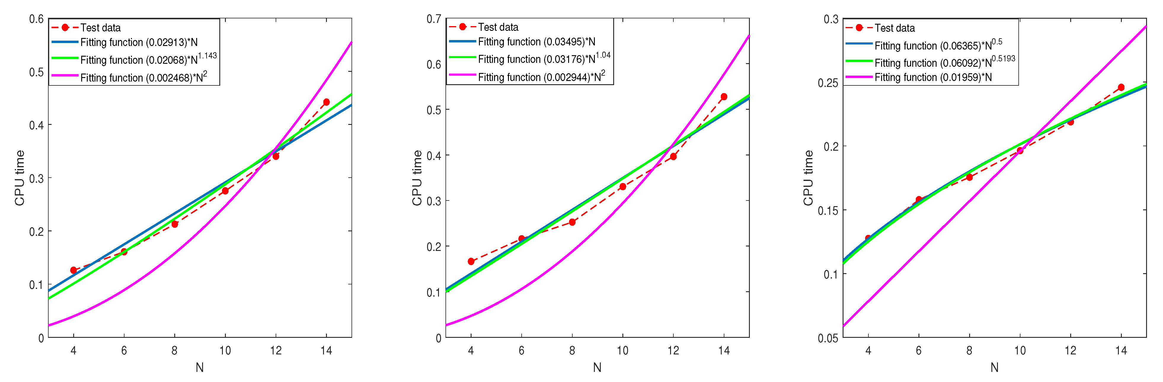
6.1. The Relationship between the CPU Time and N

In this subsection, we examine the relationship between the CPU time and parameter N using the regression technique based on the test data.

Test 9. Let $\Omega ,f,\tilde{f}$, and $\tilde{f}$ be the same as in Test 8.

Figure 9 and Figure 10 show the CPU time as a function of N obtained by the least square method and the fitting functions are given in Table 13. All the results indicate that the CPU time grew at most in the polynomial order $O\left(N^b\right)(b\le 2)$.

Figure 9. The relationship between the CPU time and parameter N when $d=5,r=3,m=1$ for computing $I_d\left(f\right)$ (left), $I_d\left(\widehat{f}\right)$ (middle), and $I_d\left(\tilde{f}\right)$ (right).

Figure 10. The relationship between the CPU time and parameter N when $d=10,r=3,m=1$ for computing $I_d\left(f\right)$ (left), $I_d\left(\widehat{f}\right)$ (middle), and $I_d\left(\tilde{f}\right)$ (right).

Table 13. The relationship between the CPU time and parameter N.

		Fitting Function $\mathit{h}\left(\mathit{N}\right)=\mathit{a}\ast {\mathit{N}}^{\mathit{b}}$
Integrand	$\mathit{d}$	$\mathit{a}$	$\mathit{b}$	$\mathit{R}$-Square	$\mathit{a}$	$\mathit{b}$	$\mathit{R}$-Square	$\mathit{a}$	$\mathit{b}$	$\mathit{R}$-Square
$f\left(x\right)$	5	0.0291	1	0.9683	0.0206	1.14	0.9790	0.0024	2	0.7361
$\widehat{f}\left(x\right)$	5	0.0349	1	0.9564	0.0317	1.04	0.9574	0.0029	2	0.6028
$\tilde{f}\left(x\right)$	5	0.0636	$\frac{1}{2}$	0.9877	0.0609	0.52	0.9889	0.0195	1	0.3992
$f\left(x\right)$	10	0.0826	1	0.9692	0.0518	1.19	0.9876	0.0070	2	0.7866
$\widehat{f}\left(x\right)$	10	0.0744	1	0.9700	0.0584	1.10	0.9758	0.0062	2	0.6905
$\tilde{f}\left(x\right)$	10	0.0373	1	0.9630	0.0558	0.83	0.9924	0.0109	$\frac{3}{2}$	0.6287

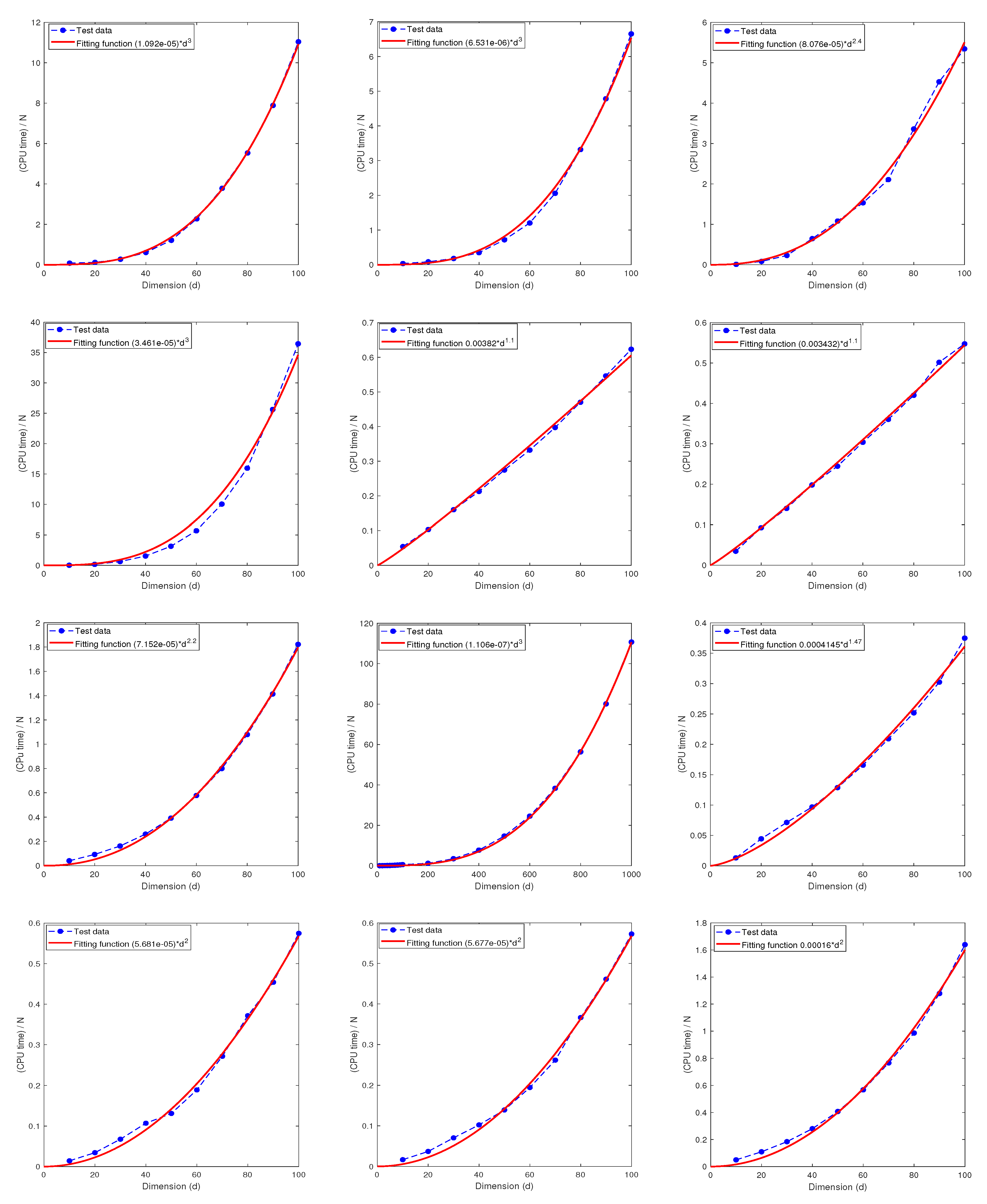
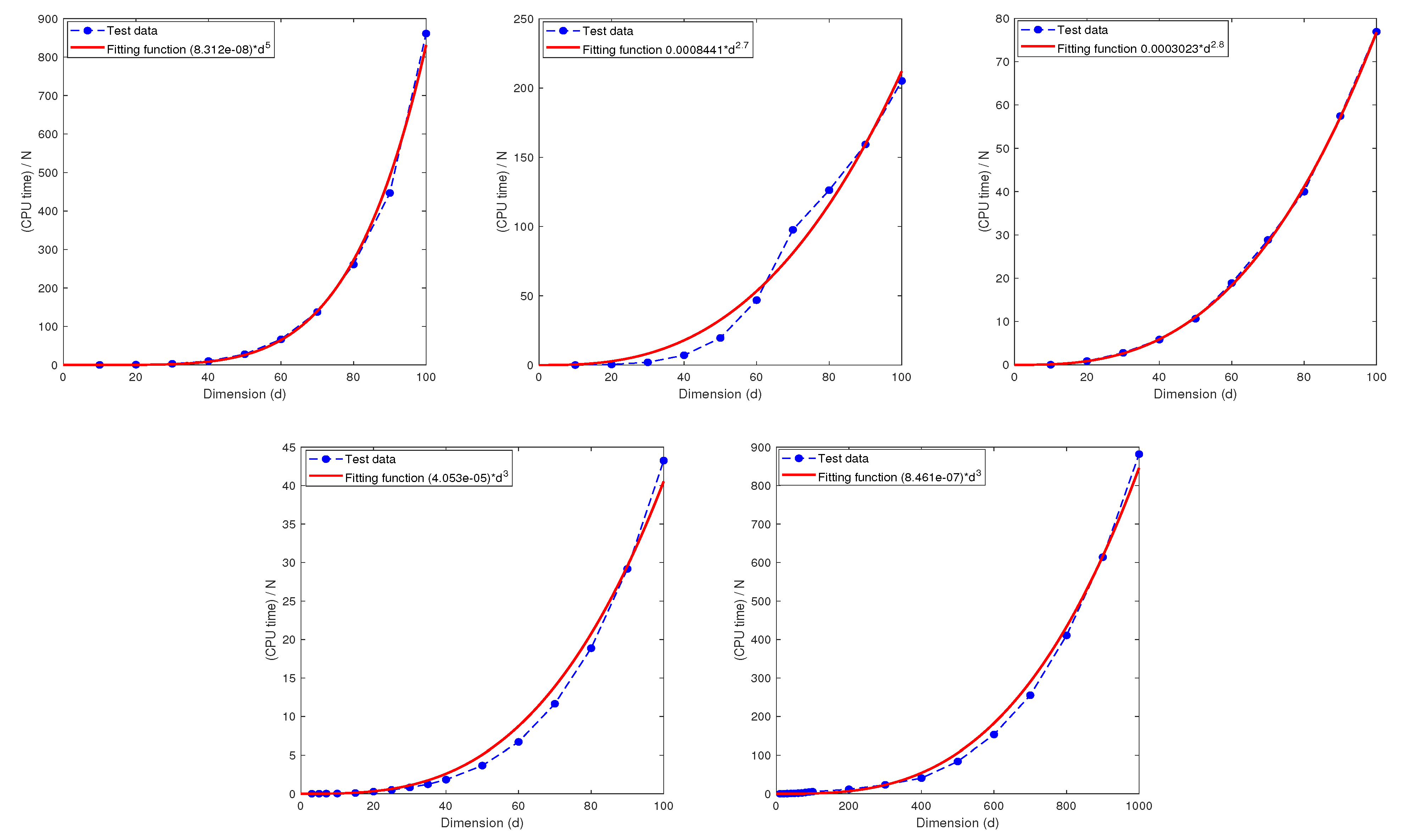
6.2. The Relationship between the CPU Time and the Dimension d

Recall that the computational complexity of the sparse grid method is of the order $O(N·{(logN)}^{d-1})$ for computing $I_d\left(f\right)$, which grew exponentially in d with base $logN$. The numerical tests presented above overwhelmingly and consistently indicate that the MDI-SG algorithm has hidden capability to overcome the curse of dimensionality, which hampers the sparse grid method. The goal of this subsection is to find out the computational complexity of the MDI-SG algorithm (in terms of CPU time as a function of d) using the regression technique based on numerical test data.

Test 10. Let $\Omega ={[0,1]}^d$ and consider the following five integrands:

$$\begin{array}{cccc}& f_1\left(x\right)=exp\left(\sum _{i=1}^d{(-1)}^{i+1}{x}_i\right),\hfill & & f_2\left(x\right)=\prod _{i=0}^d\frac{1}{0.9^2+{(x_i-0.6)}^2},\hfill \\ & f_3\left(x\right)=\frac{1}{\sqrt{2\pi }}exp\left(-\frac{1}{2}{\left|x\right|}^2\right),\hfill & & f_4\left(x\right)=cos\left(2\pi +\sum _{i=1}^d{x}_i\right),\hfill \\ & f_5\left(x\right)=\frac{1}{2^d}exp\left(\sum _{i=1}^d{(-1)}^{i+1}{x}_i\right).\hfill \end{array}$$

Figure 11 displays the CPU time as functions of d obtained by the least square regression method, whose analytical expressions are given in Table 14. We note that the parameters of the MDI-SG algorithm only affect the coefficients of the fitting functions, but not their orders in d.

Figure 11. The relationship between the CPU time and dimension d.

Table 14. The relationship between CPU time as a function of the dimension d.

Integrand	r	m	s	$\mathit{q}\left(\mathit{N}\right)$	Fitting Function	R-Square
$f_1$	1	10	1	10(33)	$g_1=(1.092e-05)\ast N{d}^3$	0.9995
	2	10	1	10(33)	$g_2=(6.531e-06)\ast N{d}^3$	0.9977
	3	10	1	10(15)	$g_3=(8.076e-05)\ast N{d}^{2.4}$	0.9946
	4	10	1	10(10)	$g_4=(3.461e-05)\ast N{d}^3$	0.9892
$f_2$	1	10	1	10(33)	$g_5=0.003820\ast N{d}^{1.1}$	0.9985
	2	10	1	10(33)	$g_6=0.003432\ast N{d}^{1.1}$	0.9986
	3	5	1	10(15)	$g_6=(7.152e-05)\ast N{d}^{2.2}$	0.9983
	3	10	1	10(15)	$g_9=(1.106e-07)\ast N{d}^3$	0.9998
	3	15	1	10(15)	$g_7=0.0004145\ast N{d}^{1.47}$	0.9955
	3	15	2	10(15)	$g_7=(5.681e-05)\ast N{d}^2$	0.9961
	3	15	3	10(15)	$g_7=(5.677e-05)\ast N{d}^2$	0.9962
	4	10	1	10(10)	$g_8=0.00016\ast N{d}^2$	0.9965
$f_3$	3	5	1	10(15)	$g_{11}=(8.312e-08)\ast N{d}^3$	0.9977
	3	10	1	10(15)	$g_{12}=0.0008441\ast N{d}^{2.7}$	0.9844
	3	15	1	10(15)	$g_{13}=0.0003023\ast N{d}^{2.8}$	0.9997
$f_4$	3	10	1	10(15)	$g_{18}=(4.053e-05)\ast N{d}^3$	0.9903
$f_5$	3	10	1	10(15)	$g_{19}=(8.461e-07)\ast N{d}^3$	0.9958

We also quantitatively characterized the performance of the fitted curve by the R-square in Matlab, which is defined as R-$\mathrm{square}=1-\frac{{\sum }_i^n{(y_i-{\widehat{y}}_i)}^2}{{\sum }_i^n{(y_i-\overline{y})}^2}$; where $y_i$ represents a test data output, ${\widehat{y}}_i$ refers to the predicted value, and $\overline{y}$ indicates the mean value of $y_i$. Table 14 also shows that the R-square of all fitting functions is very close to 1, which indicates that the fitting functions are quite accurate. These results suggest that the CPU time grows at most cubically in d. Combining the results of Test 9 in Section 6.1, we conclude that the CPU time required by the proposed MDI-SG algorithm grows at most in the polynomial order $O\left(d^3{N}^b\right)(b\le 2)$.

7. Conclusions

This paper presents an efficient and fast implementation algorithm (or solver), called the MDI-SG algorithm, for high-dimensional numerical integration using the sparse grid method. It is based on combining the idea of dimension iteration/reduction combined with the idea of computing the function evaluations at all integration points in cluster so many computations can be reused. It was shown numerically that the computational complexity (in terms of the CPU time) of the MDI-SG algorithm grows at most cubically in the dimension d, and overall in the order $O\left(d^3{N}^b\right)(b\le 2)$, where N denotes the maximum number of integration points in each coordinate direction. This shows that the MDI-SG algorithm could effectively circumvent the curse of dimensionality in high-dimensional numerical integration; hence, this shows that sparse grid methods are not only competitive but can excel in the job. Extensive numerical tests were conducted to examine the performance of the MDI-SG algorithm and to carry out performance comparisons with the standard sparse grid method and with the Monte Carlo (MC) method. It was shown that the MDI-SG algorithm (regardless of the choice of the 1-d base sparse grid quadrature rules) is faster than the MC method in low and medium dimensions (i.e., $d\lesssim 100$), much faster in very high dimensions (i.e., $d\approx 1000$), and succeeds even when the MC method fails. An immediate application of the proposed MDI-SG algorithm is to solve high-dimensional linear PDEs based on the integral equation formulation, which will be reported in a forthcoming work.

References

1. Griebel, M.; Holtz, M. Dimension-wise integration of high-dimensional functions with applications to finance. J. Complex. 2010, 26, 455–489. [Google Scholar] [CrossRef]
2. LaValle, S.M.; Moroney, K.J.; Hutchinson, S.A. Methods for numerical integration of high-dimensional posterior densities with application to statistical image models. IEEE Trans. Image Process. 1997, 6, 1659–1672. [Google Scholar] [CrossRef] [PubMed]
3. Barraquand, J.; Martineau, D. Numerical valuation of high dimensional multivariate American securities. J. Financ. Quant. Anal. 1995, 30, 383–405. [Google Scholar] [CrossRef]
4. Quackenbush, J. Extracting biology from high-dimensional biological data. J. Exp. Biol. 2007, 210, 1507–1517. [Google Scholar] [CrossRef] [PubMed]
5. Azevedo, J.D.S.; Oliveira, S.P. A numerical comparison between quasi-Monte Carlo and sparse grid stochastic collocation methods. Commun. Comput. Phys. 2012, 12, 1051–1069. [Google Scholar] [CrossRef]
6. Gerstner, T.; Griebel, M. Numerical integration using sparse grids. Numer. Algorithms 1998, 18, 209–232. [Google Scholar] [CrossRef]
7. Bungartz, H.-J.; Griebel, M. Sparse grids. Acta Numer. 2014, 13, 147–269. [Google Scholar] [CrossRef]
8. Caflisch, R.E. Monte Carlo and quasi-Monte Carlo methods. Acta Numer. 1998, 7, 1–49. [Google Scholar] [CrossRef]
9. Ogata, Y. A Monte Carlo method for high dimensional integration. Numer. Math. 1989, 55, 137–157. [Google Scholar] [CrossRef]
10. Dick, J.; Kuo, F.Y.; Sloan, I.H. High-dimensional integration: The quasi-Monte Carlo way. Acta Numer. 2013, 22, 133–288. [Google Scholar] [CrossRef]
11. Hickernell, F.J.; Müller-Gronbach, T.; Niu, B.; Ritter, K. Multi-level Monte Carlo algorithms for infinite-dimensional integration on RN. J. Complexity 2010, 26, 229–254. [Google Scholar] [CrossRef]
12. Kuo, F.Y.; Schwab, C.; Sloan, I.H. Quasi-Monte Carlo methods for high-dimensional integration: The standard (weighted Hilbert space) setting and beyond. ANZIAM J. 2011, 53, 1–37. [Google Scholar] [CrossRef]
13. Lu, J.; Darmofal, L. Higher-dimensional integration with Gaussian weight for applications in probabilistic design. SIAM J. Sci. Comput. 2004, 26, 613–624. [Google Scholar] [CrossRef]
14. Wipf, A. High-Dimensional Integrals. In Statistical Approach to Quantum Field Theory; Springer Lecture Notes in Physics; Springer: Berlin/Heidelberg, Germany, 2013; Volume 100, pp. 25–46. [Google Scholar]
15. E, W.; Yu, B. The deep Ritz method: A deep learning-based numerical algorithm for solving variational problems. Commun. Math. Stat. 2018, 6, 1–12. [Google Scholar] [CrossRef]
16. Lu, L.; Meng, X.; Mao, Z.; Karniadakis, G.E. DeepXDE: A deep learning library for solving differential equations. SIAM Rev. 2021, 63, 208–228. [Google Scholar] [CrossRef]
17. Sirignano, J.; Spiliopoulos, K. DGM: A deep learning algorithm for solving partial differential equations. J. Comput. Phys. 2018, 375, 1339–1364. [Google Scholar] [CrossRef]
18. Han, J.; Jentzen, A.E.W. Solving high-dimensional partial differential equations using deep learning. Proc. Natl. Acad. Sci. USA 2018, 115, 8505–8510. [Google Scholar] [CrossRef]
19. Xu, J. Finite neuron method and convergence analysis. Commun. Comput. Phys. 2020, 28, 1707–1745. [Google Scholar] [CrossRef]
20. Feng, X.; Zhong, H. A fast multilevel dimension iteration algorithm for high dimensional numerical integration. arXiv 2022, arXiv:2210.13658. [Google Scholar]
21. Yang, X.; Wu, L.; Zhang, H. A space-time spectral order sinc-collocation method for the fourth-order nonlocal heat model arising in viscoelasticity. Appl. Math. Comput. 2023, 457, 128192. [Google Scholar] [CrossRef]
22. Burden, R.L.; Faires, J.D. Numerical Analysis, 10th ed.; Cengage Learning: Boston, MA, USA, 2015. [Google Scholar]
23. Smolyak, S.A. Quadrature and Interpolation Formulas for Tensor Products of Certain Classes of Functions; Russian Academy of Sciences: Saint Petersburg, Russia, 1963; Volume 148, pp. 1042–1045. [Google Scholar]
24. Maruri-Aguilar, H.; Wynn, H. Sparse polynomial prediction. Stat. Pap. 2023, 64, 1233–1249. [Google Scholar] [CrossRef]
25. Deluzet, F.; Fubiani, G.; Garrigues, L.; Guillet, C.; Narski, J. Sparse grid reconstructions for Particle-In-Cell methods. ESAIM: Math. Model. Numer. Anal. 2022, 56, 1809–1841. [Google Scholar] [CrossRef]
26. Wu, J.; Zhang, D.; Jiang, C. On reliability analysis method through rotational sparse grid nodes. Mech. Sys. Signal Process. 2021, 147, 107106. [Google Scholar] [CrossRef]
27. Baszenki, G.; Delvos, F.-J. Multivariate Boolean Midpoint Rules, Numerical Integration IV; Birkhäuser: Basel, Switzerland, 1993; pp. 1–11. [Google Scholar]
28. Paskov, S.H. Average case complexity of multivariate integration for smooth functions. J. Complex. 1993, 9, 291–312. [Google Scholar] [CrossRef]
29. Bonk, T. A new algorithm for multi-dimensional adaptive numerical quadrature. In Adaptive Methods—Algorithms, Theory and Applications; Vieweg/Teubner Verlag: Wiesbaden, Germany, 1994; pp. 54–68. [Google Scholar]
30. Novak, E.; Ritter, K. The curse of dimension and a universal method for numerical integration. In Multivariate Approximation and Splines; Birkhäuser: Basel, Switzerland, 1997; pp. 177–187. [Google Scholar]
31. Novak, E.; Ritter, K. High dimensional integration of smooth functions over cubes. Numer. Math. 1996, 75, 79–97. [Google Scholar] [CrossRef]
32. Patterson, T.N.L. The optimum addition of points to quadrature formulae. Math. Comp. 1968, 22, 847–856. [Google Scholar] [CrossRef]
33. Novak, E.; Ritter, K. Simple Cubature Formulas for d-Dimensional Integrals with High Polynomial Exactness and Small Error; Report; Institut für Mathematik, Universität Erlangen–Nürnberg: Nürnberg, Germany, 1997. [Google Scholar]