Z-Type Control Methods on a Three-Species Model with an Invasive Prey

Abstract

The process by which nature and evolution discriminate between species bound to survive or become extinct has always been an interesting phenomenon. One example of this selection is represented by biological invasions, when alien species spread into new environments causing ecological disruptions, alteration of native population dynamics and ecosystem dysfunctioning. In this paper, we concentrate on the introduction of the Eastern cottontail (Sylvilagus floridanus) into the regions of northern and central Italy. This has influenced the local predator–prey dynamics of the indigenous European hares (Lepus europaeus) and red foxes (Vulpes vulpes), consequently producing a “hyperpredation” effect on hares. In this framework, we investigate this scenario with the objective of mitigating the negative effects of the invasion. Specifically, we devise and apply a Z-control technique in order to drive chosen populations toward a desired state that at least theoretically can ensure the survival of native species. The purpose of such a study is twofold: on one hand, this approach is employed with the aim of reducing the invasive population; secondly, it aims to avoid the extinction of native prey, i.e., the hare population.

1. Introduction

Currently, with global communications a phenomenon unknown in centuries before the XXth is occurring, also favored by the ongoing climatic changes. It is represented by the invasions of alien species that find new habitats in regions where they were formerly unknown [1]. The negative effects of alien species on indigenous ones can be exerted in various ways [2]. For example, demographically, by competition, predation or hybridization, and epidemiologically, via new disease transmission. In particular, during the invasion the alien species often outcompete the native ones, for various reasons, among which we can mention the larger niche occupied by the invaders, their bigger size, absence of specific predators and so on. The alien species may also become a nuisance for agriculture, in addition to the indigenous species [3,4,5].

Modeling pest populations is a fundamental task for biological control, which tries to fight these pernicious agents via their natural enemies, rather than by using chemicals. In the last decades, the latter have indeed often been found to produce counterproductive effects [6]. Focusing on insects, spraying also kills useful populations, such as spiders, generalist predators that remove a very sizeable quantity of insects [7,8,9]. A second side effect is that upon ingestion by other animals that are not their specific target, these poisons enter into the food web, accumulating in the largest animals. Indeed, the latter have longer lifespans and therefore their intake lasts longer and may ultimately reach dangerous levels in their bodies. Through the passage among various trophic levels, these poisons end up on our tables and finally in our bodies. This advocates the use of alternative methods, such as biological control [10,11,12,13,14].

The output of population model studies is the assessment of the final regime of the dynamical system, e.g., stable equilibria configurations or persistent oscillations. The theoretical analysis allows one to assess under which conditions these configurations occur, in terms of the model parameters. Often, it is the case that these various situations are linked to each other, in the sense that a change of a parameter shifts the ecosystem to a different outcome. The latter can be induced by natural stochastic environmental fluctuations or by temperature or other physical quantity changes brought up by different climatic conditions. It is sometimes possible to obtain a chart in which all the final system configurations appear, with links among “neighboring” equilibria, i.e., those attainable by a parameter change. Such a graph would represent a useful tool for ecosystem managers to drive ecosystems toward a desired state [15].

In this paper, we turn our attention to the introduction of an invasive species into a predator–prey system. This in general can lead to direct or indirect competition between native and exotic species, which in some cases can even lead to the extinction of one or more native species [16]. In this regard, let us keep in mind that invasive species are a major cause of animal extinction [17]. Several ecological implications of invasions have been analyzed in the literature, for example, in the case of marine invaders in [18] and of terrestrial invaders in [19].

In particular, we consider a specific invasion situation concerning the Eastern cottontail (Sylvilagus floridanus). This lagomorph has shifted the natural equilibrium between red foxes (Vulpes vulpes) and native European hares (Lepus europaeus) in the northern and central regions of Italy [20,21,22]. No direct competition seems to occur between the hares and the cottontails. However, indirect competition dynamics exist between the two lagomorphs. In fact, the correlation between fox and hare abundances, which is positive when invasive rodents are few, becomes more and more negative as the latter’s population increases [23]. A theoretical investigation has allowed an explanation of the phenomenon [24]. However, the problem persists. An increase in cottontail abundance would lead to an increase in fox populations, amplifying their predatory impact on hares (“hyperpredation”). Alternatively, cottontails attract foxes where they live and where there are also important resting areas for hares, and consequently the increased presence of foxes results in increased predation rates on hares. In order to preserve the native hare, it is necessary to control the invader population. For this task, we apply a relatively novel technique, the Z control [25,26,27,28].

The article is organized as follows. In the next section, the Z-control technique is recalled, the reference model on which to apply this technique is presented and finally, three different indirect control strategies are proposed, respectively, in Section 2.3, Section 2.4 and Section 2.5: action on foxes, action on hares and combined action on foxes and hares. Each one of the new models is studied analytically in detail. In particular, the possible equilibrium points are determined with their feasibility and local stability conditions. In the case of action on foxes, a transcritical bifurcation linking the hare-free equilibrium with coexistence has also been identified, analytically demonstrated and graphically represented. In Section 3, several numerical simulations obtained using MATLAB are shown. Further, the biological interpretation of the three proposed controls is discussed. The Conclusion finally debates the best option to manage the ecological control problem.

2. Materials and Methods

2.1. Highlights on the Z Control

Starting from an autonomous system $\dot{\mathbf{y}}=f(\mathbf{y},\mathbf{G})$ incorporating an unknown control function $\mathbf{G}=\mathbf{G}\left(t\right)$ as input, the central idea of the Z control method is to consider the evolution over time of the tracking error function ${\mathbf{v}}_1\left(t\right)=\mathbf{y}\left(t\right)-{\mathbf{y}}_d\left(t\right)$, which measures the discrepancy between the output solution $\mathbf{y}\left(t\right)$ and the desired outcome ${\mathbf{y}}_d\left(t\right)$. More in detail, this method is based on forcing the first error ${\mathbf{v}}_1\left(t\right)$ to converge zero exponentially in the following prescribed way:

$${\displaystyle \frac{d{\mathbf{v}}_1}{dt}}\left(t\right)=-\lambda {\mathbf{v}}_1\left(t\right).$$

(1)

If it is not possible to find an explicit expression for the control function $\mathbf{G}\left(t\right)$ from Equation (1), the same process is repeated for the subsequent errors ${\mathbf{v}}_k\left(t\right)$, recursively defined by

$${\mathbf{v}}_k\left(t\right)≔{\displaystyle \frac{d{\mathbf{v}}_{k-1}}{dt}}\left(t\right)+\lambda {\mathbf{v}}_{k-1}\left(t\right),k\ge 2,$$

until this goal is achieved. This means that, at each step, a new condition is imposed:

$${\displaystyle \frac{d{\mathbf{v}}_k}{dt}}\left(t\right)=-\lambda {\mathbf{v}}_k\left(t\right).$$

The control function can involve one or more equations of the original model. We distinguish between indirect and direct controls. In the former case, the equations of the classes to be controlled are not modified and the action is performed on other classes; in the second case, a control function is introduced directly on the classes for which a desired state has been chosen.

In our case, this method will be applied in three different ways, namely, acting on the foxes alone with the aim of reducing the invasive population and possibly to avoid the extinction of native hares; alternatively just acting on the hares to preserve them and possibly eradicate the cottontails; finally, by combining these efforts.

2.2. The Reference Model

The starting point of this analysis is a three-species mathematical model (sometimes referred to simply as reference model) which describes the predator–two-prey interaction between the two native species, foxes and hares, and the invasive cottontail species. As already mentioned, the model formulated in [24] has explained the field results obtained in [23].

Formally, the dynamics are described by the following system of first-order nonlinear ordinary differential equations, where the variables V, S and L, respectively, represent the populations of foxes, cottontails and hares:

$$\begin{array}{c}\hfill \begin{array}{cc}& {\displaystyle \frac{dV}{dt}}=V(r-c_{VV}V-m+eaS+ebL)=f_1(V,S,L),\hfill \\ & {\displaystyle \frac{dS}{dt}}=S(s-c_{SS}S-n-aV)=f_2(V,S),\hfill \\ & {\displaystyle \frac{dL}{dt}}=L(u-c_{LL}L-p-bV)=f_3(V,L).\hfill \end{array}\end{array}$$

(2)

All parameters are nonnegative, with their values being taken from [24], unless otherwise specified. In particular, information from [20,21,22] on the hares’ carrying capacity allows the determination of the intraspecific competition rate for this species. These equations essentially model reproduction and intraspecific competition for all species, natural mortality and the hunting of foxes over the two types of prey. These interactions are described via mass action, or Holling type I, terms in view of the low population densities. It is important to remark that direct interspecific competition between prey does not occur, as clearly discussed in [24].

A preliminary analysis of the model leads to eight equilibria $E_i=(V_i,S_i,L_i)$ for $i=0,\dots ,7$, whose feasibility conditions and stability properties can be found in [24]; for our discussion, we will just consider

$$E_3=({\displaystyle \frac{ae(s-n)+c_{SS}(r-m)}{a^{2}e+c_{VV}{c}_{SS}}},{\displaystyle \frac{a(m-r)+c_{VV}(s-n)}{a^{2}e+c_{VV}{c}_{SS}}},0),$$

$$E_4=(0,0,{\displaystyle \frac{u-p}{c_{LL}}}),$$

$$E_5=({\displaystyle \frac{be(u-p)+c_{LL}(r-m)}{b^{2}e+c_{VV}{c}_{LL}}},0,{\displaystyle \frac{b(m-r)+c_{VV}(u-p)}{b^{2}e+c_{VV}{c}_{LL}}})$$

(where the names are referred to the ones in [24]) in order to facilitate a comparison with the models in which Z-control is applied. In addition to explaining the “hyperpredation effect” empirically observed, the results of the analysis of [24] show that coexistence of the three species is possible under suitable conditions, but also that the extinction of the hares can occur. In the former case, this means persistence of the invader. Our task here is to try to curb this phenomenon and possibly to enhance the hares’ survival. This is performed in three different ways: acting separately on foxes, at first, then on the hare population and finally by a combination of the two.

2.3. Invasive Species Removal: Single Indirect Control on Foxes

Here, we apply an indirect control on the cottontail population acting on foxes. This is performed by introducing a control function $G\left(t\right)$ in the equation of the foxes. The motivation behind this choice lies in the fact that to curb the invasive cottontails causing the hyperpredation effect on hares, a predator removal is considered, thereby reducing the pressure on hares. The class to be forced is represented by the cottontails S, for which the desired state is here chosen as a nonnegative constant function $S_d\left(t\right)\equiv S_d$$\forall t\ge 0$, with $S_d\approx 0$.

2.3.1. Z-Controlled Model Design on Foxes

The first modified model is obtained acting on the first equation of the reference model (2) by introducing a forcing function $G_{\mathrm{pred}}\left(t\right)$, while the other two equations remain unchanged:

$${\displaystyle \frac{dV}{dt}}=f_1(V,S,L)-G_{\mathrm{pred}}\left(t\right)V.$$

(3)

From now on, we will refer to it as $G\left(t\right)$ for simplicity. In general, the input function could assume both positive and negative values, but what is considered relevant in this context is $G\left(t\right)>0$. This function could possibly represent a culling or removal of predators followed by their transfer elsewhere.

Introducing now a design parameter

$$\lambda >0,$$

we define the first error function

$$v_1\left(t\right)≔S\left(t\right)-S_d\left(t\right).$$

(4)

We apply the Z-control method by imposing $v_1\left(t\right)$ to approach 0 exponentially fast for $t\to +\infty$. This corresponds to setting

$$\frac{d{v}_1}{dt}\left(t\right)=-\lambda v_1\left(t\right).$$

In this case, we will also need a further condition involving the second error function, defined as

$$v_2\left(t\right)≔{\displaystyle \frac{d{v}_1}{dt}}\left(t\right)+\lambda v_1\left(t\right)$$

(5)

so that an explicit expression of the control function $G\left(t\right)$ can be found in the following way. Imposing once more

$$\frac{d{v}_2}{dt}\left(t\right)=-\lambda v_2\left(t\right)$$

and substituting in it (5), we are led to

$$\frac{d^2{v}_1}{d{t}^2}\left(t\right)+\lambda \frac{d{v}_1}{dt}\left(t\right)=-\lambda [\frac{d{v}_1}{dt}\left(t\right)+\lambda v_1\left(t\right)]$$

and finally to

$$\frac{d^2{v}_1}{d{t}^2}\left(t\right)+2\lambda \frac{d{v}_1}{dt}\left(t\right)+{\lambda }^2{v}_1\left(t\right)=0.$$

(6)

It is now sufficient to rewrite (6) in terms of the original variables, omitting for convenience the dependence on t, to obtain

$$(\frac{d^{2}S}{d{t}^2}-\frac{d^2{S}_d}{d{t}^2})+2\lambda (\frac{dS}{dt}-\frac{d{S}_d}{dt})+{\lambda }^2(S-S_d)=0$$

and rearranging

$$\frac{d^{2}S}{d{t}^2}+2\lambda \frac{dS}{dt}+{\lambda }^{2}S-(\frac{d^2{S}_d}{d{t}^2}+2\lambda \frac{d{S}_d}{dt}+{\lambda }^2{S}_d)=0.$$

By letting

$$G_d\left(t\right)=\frac{d^2{S}_d}{d{t}^2}\left(t\right)+2\lambda \frac{d{S}_d}{dt}\left(t\right)+{\lambda }^2{S}_d\left(t\right)$$

(7)

and observing that

$$\frac{d^{2}S}{d{t}^2}={\displaystyle \frac{d{f}_2}{dV}}\frac{dV}{dt}+{\displaystyle \frac{d{f}_2}{dS}}\frac{dS}{dt}=-aS[f_1-G\left(t\right)V]+(s-2S{c}_{SS}-n-aV)f_2,$$

we thus obtain

$$-aS{f}_1+aSVG\left(t\right)+(s-2S{c}_{SS}-n-aV+2\lambda )f_2+{\lambda }^{2}S-G_d\left(t\right)=0.$$

(8)

We now solve in terms of G Equation (8) to get the control function

$$G_{\mathrm{pred}}\left(t\right)=G_{\lambda }\left(t\right)+{\displaystyle \frac{G_d\left(t\right)}{aSV}}\mathrm{with}{G}_{\lambda }\left(t\right)={\displaystyle \frac{f_1}{V}}-{\displaystyle \frac{f_2(f_2-c_{SS}{S}^2+2\lambda S)}{a{S}^{2}V}}-{\displaystyle \frac{{\lambda }^2}{aV}}.$$

(9)

Note that in so doing we must assume $S,V\ne 0$. This is the reason why we cannot impose that $S_d=0$. From (7), we finally observe that for $S_d\left(t\right)\equiv S_d=\mathrm{const}.$ the expression of $G_d\left(t\right)$ simplifies to $G_d\left(t\right)\equiv {\lambda }^2{S}_d$. Furthermore, substituting (9) into (3), we obtain

$$\frac{dV}{dt}={\displaystyle \frac{f_2(f_2-c_{SS}{S}^2+2\lambda S)}{a{S}^2}}+{\displaystyle \frac{{\lambda }^2}{a}}-{\displaystyle \frac{G_d}{aS}}=F_1(V,S).$$

Note that the equation describing the dynamics of foxes in the model controlled in this way explicitly depends not only on V but also on S.

Theorem 1. 

For any positive initial state $(V_0,S_0,L_0)$ and for any continuously differentiable and bounded desired state $S_d\left(t\right)$, the tracking error function $v_1\left(t\right)$ converges to zero exponentially.

Proof. 

We observe that setting $u_1=v_1$ and $u_2={\dot{v}}_1$, (6) is equivalent to the following system of first-order equations

$$\begin{array}{c}\hfill \begin{array}{cc}& {\dot{u}}_1\left(t\right)=u_2,\hfill \\ & {\dot{u}}_2\left(t\right)=-{\lambda }^2{u}_1-2\lambda u_2.\hfill \end{array}\end{array}$$

This system has the general solution

$$v_1\left(t\right)=c_1{e}^{-\lambda t}+c_{2}t{e}^{-\lambda t}$$

where, using the initial conditions

$$\begin{array}{cc}\hfill & c_1=S\left(0\right)-S_d\left(0\right),\hfill \\ \hfill & c_2=\dot{S}\left(0\right)-{\dot{S}}_d\left(0\right)+\lambda [S\left(0\right)-S_d\left(0\right)].\hfill \end{array}$$

Applying Lemma 1 of [29], it is possible to control with an exponential function the term $c_{2}t{e}^{-\lambda t}$ appearing in the expression of $v_1\left(t\right)$. Choosing $C,\Lambda >0$ appropriately, we can then bound $v_1\left(t\right)$ from above

$$v_1\left(t\right)\le C{e}^{-\Lambda t}\forall t\ge 0.$$

From this, the exponential convergence of the error to zero with rate $\lambda$ is proved. □

2.3.2. Equilibria

We now look for the equilibrium points of the controlled system and study their feasibility conditions, excluding the cases in which either V or S vanish, as stated above. The only population that is theoretically allowed to disappear is thus L. The equilibrium equations lead only to the two possible equilibria

$$E_L=(\widehat{V},\widehat{S},0)\mathrm{and}{E}_c=(\widehat{V},\widehat{S},\widehat{L})$$

where

$$\begin{array}{c}\hfill \widehat{V}={\displaystyle \frac{{\lambda }^2(s-n)-c_{SS}{G}_d}{a{\lambda }^2}},\widehat{S}={\displaystyle \frac{s-n-a\widehat{V}}{c_{SS}}}={\displaystyle \frac{G_d}{{\lambda }^2}},\\ \hfill \widehat{L}={\displaystyle \frac{u-p-bV}{c_{LL}}}={\displaystyle \frac{a{\lambda }^2(u-p)-b{\lambda }^2(s-n)+b{c}_{SS}{G}_d}{a{\lambda }^2{c}_{LL}}}.\end{array}$$

Observe that $\widehat{S}=S_d$ when $G_d\left(t\right)\equiv {\lambda }^2{S}_d$, which is consistent with the control requesting $S\left(t\right)$ to achieve a stationary state. Furthermore, the value of $\widehat{V}$ at both equilibria is the same. It depends only on the choice of $S_d$. Hence, the only difference between these points is determined by the survival or extinction of the hare population. As far as these two equilibria are concerned, the first one does not reflect an optimal ecological situation, as the hares disappear while foxes, being generalist predators, would be supported not only by cottontails but also by the alternative feeding resources modeled via the carrying capacity in System (2). Instead, the second one is preferable because “near extinction”, if $S_d\approx 0$, only affects the invasive species. There is the possibility then that the pristine invader-free ecosystem could be restored.

We rewrite here for convenience the actual populations at equilibrium with the specific choice of $S_d\left(t\right)\equiv S_d=\mathrm{const}.$

$$\widehat{V}={\displaystyle \frac{(s-n)-c_{SS}{S}_d}{a}},\widehat{S}=S_d,\widehat{L}={\displaystyle \frac{a(u-p)-b(s-n)+b{c}_{SS}{S}_d}{a{c}_{LL}}}.$$

Finally, the equilibria have biological sense if the populations are nonnegative. Thus, the following feasibility conditions for $E_L$ must hold:

$$s\ge n+c_{SS}{S}_d,S_d>0,$$

(10)

while those for $E_c$ are

$$s\ge n+c_{SS}{S}_d,S_d>0,a(u-p)\ge b[(s-n)-c_{SS}{S}_d].$$

(11)

If not otherwise specified, from now on we will assume they are verified. As already remarked earlier, an important point is that $S_d\ne 0$.

2.3.3. Local Stability Analysis

For a local stability analysis, we consider the matrix of the linearized system in a neighborhood of each equilibrium point, i.e. the Jacobian matrix evaluated at each equilibrium. Some derivatives are indeed immediate, since $F_1,f_2$ and $f_3$ do not depend on L and S, respectively.

The Jacobian matrix of the Z-controlled model is

$$\widehat{J}=\left(\begin{array}{ccc}{\displaystyle \frac{d{F}_1}{dV}}& {\displaystyle \frac{d{F}_1}{dS}}& 0\\ -aS& {\displaystyle \frac{d{f}_2}{dS}}& 0\\ -bL& 0& {\displaystyle \frac{d{f}_3}{dL}}\end{array}\right),$$

(12)

so that its characteristic polynomial factorizes to immediately provide an explicit real eigenvalue ${\mu }_1={\displaystyle \frac{d{f}_3}{dL}}$, while the remaining ones come from the roots of the quadratic

$$P\left(\mu \right)=\sum _{i=0}^2{a}_i{\mu }^i=0,a_1=-(\frac{d{F}_1}{dV}+\frac{d{f}_2}{dS}),a_0=\frac{d{F}_1}{dV}\frac{d{f}_2}{dS}+aS\frac{d{F}_1}{dS}.$$

In addition to the negativity of ${\mu }_1$, the local stability for the equilibria is obtained by applying the Routh–Hurwitz (RH) criterion.

Proposition 1. 

For the Z-controlled Models (2) and (3):

• If feasible, the hare-free equilibrium $E_L$ is locally asymptotically stable if and only if

  $$u-p-b\widehat{V}<0;$$

  (13)
• The coexistence equilibrium $E_c$, when feasible, is instead locally asymptotically stable for every choice of parameters, including λ.

Proof. 

The asymptotic local stability for the equilibria is therefore equivalent to requiring the RH conditions on the principal minor of (12), $\mathrm{tr}\left(\widehat{J}\right)<0$ and $det\left(\widehat{J}\right)>0$, which are the same for both equilibria and unconditionally satisfied, as for all $\lambda >0$

$$a_1=-\mathrm{tr}\left(\widehat{J}\right)=2\lambda >0,a_0={\lambda }^2>0.$$

Hence, the stability is determined by the sign of the first eigenvalue, for which we distinguish the two cases. For $E_L$

$${\mu }_1^{\left(L\right)}=\frac{d{f}_3}{dL}\left(E_L\right)=u-p-b\widehat{V},$$

and for $E_c$

$${\mu }_1^{\left(c\right)}=\frac{d{f}_3}{dL}\left(E_c\right)=-c_{LL}\widehat{L}<0,$$

which holds unconditionally.

In conclusion, stability for $E_c$ is unconditional when it is feasible, namely, (11) holds, while for $E_L$ in addition to feasibility (10) it is also necessary to require (13). □

From the two previous properties, the bifurcation scenarios may be discussed, taking as bifurcation parameter, for instance, b. Choosing for b a value much larger than the one of a could represent a hyperpredation situation. Such a choice may produce stability for $E_L$, as the hare population is subject to a higher pressure.

Assume that all ecological parameters are fixed so that the feasibility conditions of $E_L$ are satisfied. Studying the sign change of $a(u-p-b\widehat{V})=a(u-p)-b(s-n)-b{c}_{SS}{S}_d$, we can find the critical value $b^{*}$ for a local stability transition of $E_L$:

$$b^{*}=a{\displaystyle \frac{u-p}{s-n-c_{SS}{S}_d}}.$$

Note that some values of b do not guarantee the feasibility of $E_c$. Specifically, (11) are not satisfied if $b\ge b^{*}$.

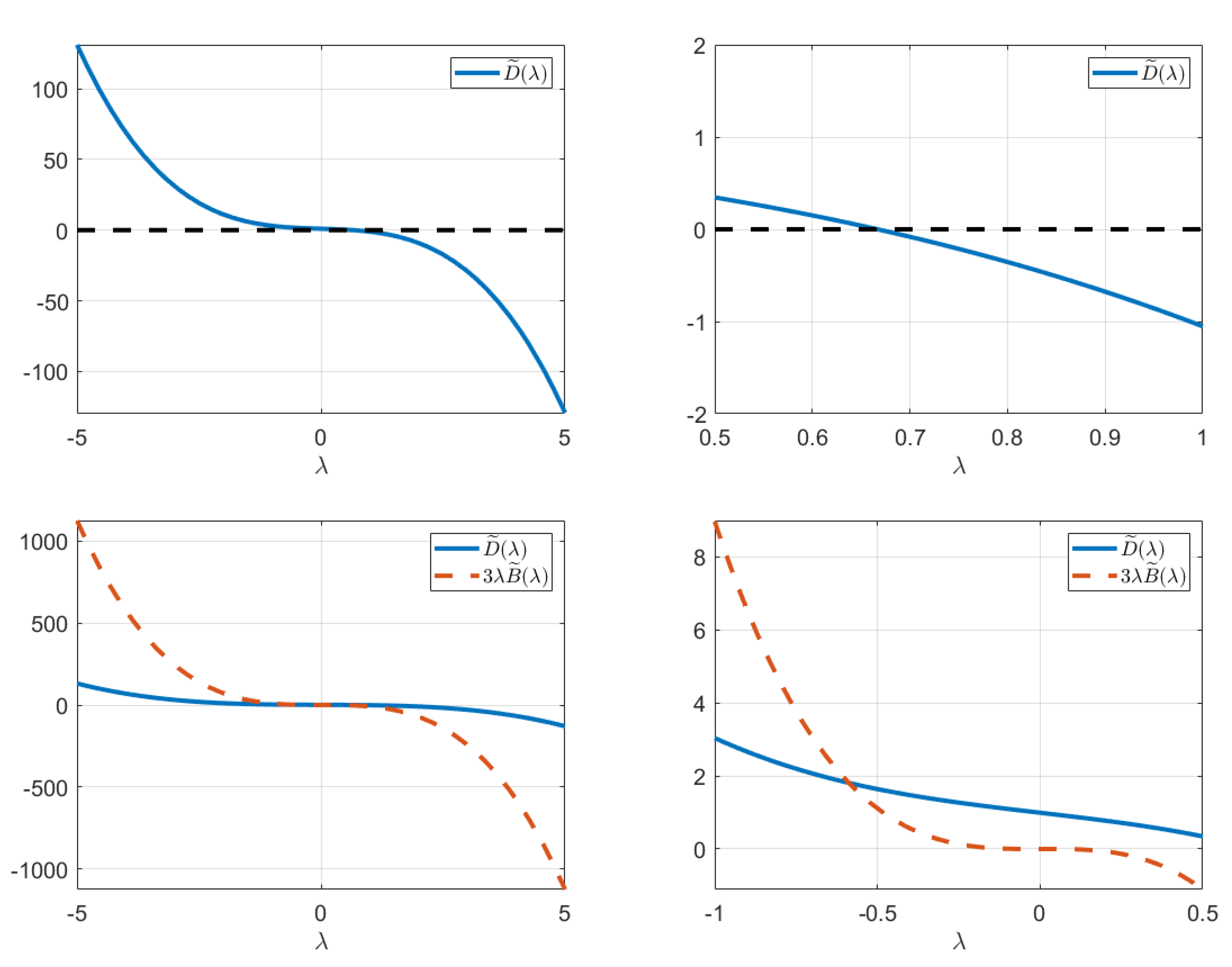
2.3.4. Existence of the Transcritical Bifurcation

We now actually prove the existence of the transcritical bifurcation for which $E_L$ emanates from $E_c$ as soon as b increases past $b^{*}$, using the classical tool of Sotomayor’s theorem [30].

Evaluating in $E_L$ the Jacobian matrix $\widehat{J}$ of the Z-controlled model with $S_d\left(t\right)\equiv S_d=\mathrm{const}.$, we obtain

$$\widehat{J}\left(E_L\right)=\left(\begin{array}{ccc}{c}_{SS}{S}_d-2\lambda & \frac{c_{SS}(c_{SS}{S}_d-2\lambda )}{a}+\frac{{\lambda }^2}{a{S}_d}& 0\\ -a{S}_d& -c_{SS}{S}_d& 0\\ 0& 0& u-p-\frac{b(s-n-c_{SS}{S}_d)}{a}\end{array}\right).$$

Focusing attention on the parameter b, we can observe that the third element on the diagonal of $\widehat{J}\left(E_L\right)$ vanishes when $b=b^{*}$, and in view of the structure of $\widehat{J}\left(E_L\right)$, it is in fact an eigenvalue. Right and left eigenvectors of $\widehat{J}(E_L,b^{*})$ are $v=w={\left[0,0,1\right]}^T.$ Furthermore, denoting by F the system’s right-hand side, we find

$$F_b={[0,0,-VL]}^T\mathrm{and}D{F}_b=\left[\begin{array}{ccc}0& 0& 0\\ 0& 0& 0\\ -L& 0& -V\end{array}\right].$$

Consequently, we have

$$w^T{F}_b(E_L,b^{*})=0,w^T\left[D{F}_b(E_L,b^{*})v\right]=-\widehat{V}\ne 0\iff S_d\ne \frac{s-n}{c_{SS}}$$

and

$$w^T\left[D^{2}F(E_L,b^{*})(v,v)\right]=D^2{f}_3(E_L,b^{*})(v,v)=\frac{d^2{f}_3}{d{L}^2}(E_L,b^{*})v_3^2=-2c_{LL}\ne 0.$$

Thus, Sotomayor’s theorem allows us to conclude that if $s\ne n$, there is a transcritical bifurcation from $E_c$ to $E_L$ at $b=b^{*}$.

This transcritical bifurcation is graphically represented in Figure 1. The initial conditions are

$$V\left(0\right)=0.4,S\left(0\right)=1\mathrm{and}L\left(0\right)=3,$$

(14)

while the ecological parameter values are those of [24], except b, which are

$$\begin{array}{cc}\hfill & a=0.2,c_{VV}=log\left(3\right)-\frac{2}{7},c_{SS}=\frac{log\left(4.5\right)}{100}-\frac{4}{500},\hfill \\ \hfill & c_{LL}=\frac{log\left(5\right)}{30}-\frac{2}{330},e=0.91,m=\frac{2}{7},n=\frac{4}{5},p=\frac{2}{11},\hfill \\ \hfill & r=log\left(3\right),s=log\left(4.5\right)\mathrm{and}u=log\left(5\right).\hfill \end{array}$$

(15)

In this case, we choose $S_d=0.5\ne \frac{s-n}{c_{SS}}=100$ and $\lambda =0.01$ and we vary the parameter b in the interval $[0,1]$. The transcritical bifurcation from $E_c$ to $E_L$ occurs at the critical value $b=b^{*}\approx 0.4076$.

2.4. Action on Hares

In view of the hyperpredation effect on hares exerted by foxes in the presence of the invading cottontails [23,24], it is imperative to find ways of curbing this negative effect.

For this second scenario, the goal remains the same, but in this case instead of culling the predators, the importation of hares from outside is assumed. This sustains the hare population, although it also provides more resources for foxes. However, one should keep in mind that the introduction of alien hares may have a negative effect on the native population, with the possible emergence of a new hybrid species and the pushing of the native one toward smaller and more inhospitable areas, as discussed in [31].

We now consider the second approach for indirect control of cottontail population. We introduce an unknown input function $G_{\mathrm{prey}}\left(t\right)$, to modify the reference Model (2) so that now the last equation becomes

$${\displaystyle \frac{dL}{dt}}=f_3(V,L)+G_{\mathrm{prey}}\left(t\right)L=F_3,$$

(16)

while the other two equations are the same as in (2). From now on we will refer to $G_{\mathrm{pred}}\left(t\right)$ as $\tilde{G}\left(t\right)$ for simplicity. The idea behind this choice is that we consider an additional “immigration” term for hares in order to preserve them from extinction. We apply the Z-control method to drive $S\left(t\right)$ to the desired state $S_d$. Since $\tilde{G}\left(t\right)$ is part of the third equation, we need to impose error conditions mathematically until the derivative of L with respect to time is involved. In particular, we prove that by repeating the Z-control process up to the third error, an explicit expression for $\tilde{G}\left(t\right)$ can be obtained.

Recalling (4) and (5), we define the third error function as follows

$$v_3\left(t\right)≔\frac{d{v}_2}{dt}\left(t\right)+\lambda v_2\left(t\right)$$

and impose once again

$$\frac{d{v}_3}{dt}\left(t\right)=-\lambda v_3\left(t\right).$$

Back substitution now leads to

$${\displaystyle \frac{d^3{v}_1}{d{t}^3}}\left(t\right)+3\lambda {\displaystyle \frac{d^2{v}_1}{d{t}^2}}\left(t\right)+3{\lambda }^2{\displaystyle \frac{d{v}_1}{dt}}\left(t\right)+{\lambda }^3{v}_1\left(t\right)=0.$$

Rewriting it in terms of S, we obtain

$${\displaystyle \frac{d^{3}S}{d{t}^3}}+3\lambda {\displaystyle \frac{d^{2}S}{d{t}^2}}+3{\lambda }^2{\displaystyle \frac{dS}{dt}}+{\lambda }^{3}S-{\tilde{G}}_d\left(t\right)=0,$$

with

$${\tilde{G}}_d\left(t\right)={\displaystyle \frac{d^3{S}_d}{d{t}^3}}\left(t\right)+3\lambda {\displaystyle \frac{d^2{S}_d}{d{t}^2}}\left(t\right)+3{\lambda }^2{\displaystyle \frac{d{S}_d}{dt}}\left(t\right)+{\lambda }^3{S}_d\left(t\right),$$

from which an explicit expression $G_{\mathrm{prey}}\left(t\right)$ is obtained for $SVL\ne 0$

$$G_{\mathrm{prey}}\left(t\right)=\frac{1}{abeSVL}[{\tilde{G}}_{\lambda }\left(t\right)-{\tilde{G}}_d\left(t\right)]-{\displaystyle \frac{f_3}{L}},$$

where

$$\begin{array}{c}\hfill {\tilde{G}}_{\lambda }\left(t\right)=-aS{\displaystyle \frac{f_1^2}{V}}-2f_2^2{c}_{SS}-3a{f}_1{f}_2+aS(c_{VV}V+c_{SS}S-3\lambda )f_1+\\ \hfill +\left[\right({\displaystyle \frac{f_2}{S}}-c_{SS}S{)}^2+3\lambda ({\displaystyle \frac{f_2}{S}}-c_{SS}S)+3{\lambda }^2-e{a}^{2}SV]f_2+{\lambda }^{3}S.\end{array}$$

We can therefore rewrite the right-hand side of the third equation more conveniently as:

$$F_3=\frac{1}{abeSV}[{\tilde{G}}_{\lambda }\left(t\right)-{\tilde{G}}_d\left(t\right)].$$

2.4.1. Equilibria

For this model as well, we search for possible stationary configurations. Solving the equilibrium equations leads to a unique coexistence equilibrium $\tilde{E}=(\tilde{V},\tilde{S},\tilde{L})$ since all the populations cannot be zero. Assuming ${\tilde{G}}_d\left(t\right)$ to be constant, the coexistence population values are

$$\tilde{V}={\displaystyle \frac{(s-n)-c_{SS}{S}_d}{a}},\tilde{S}={\displaystyle \frac{s-n-a\tilde{V}}{c_{SS}}}={\displaystyle \frac{{\tilde{G}}_d\left(t\right)}{{\lambda }^3}}=S_d,$$

$$\tilde{L}={\displaystyle \frac{-a(r-m)+c_{VV}(s-n)-(c_{VV}{c}_{SS}+e{a}^2)S_d}{abe}}.$$

(17)

Once again, we observe that by forcing the solution $S\left(t\right)$, at equilibrium we obtain a value of $\tilde{S}=S_d$, which cannot be zero. The feasibility conditions for $\tilde{V}$ and $\tilde{S}$ are the same as (11), while for the third one $\tilde{L}>0$, we now obtain

$$c_{VV}[(s-n)-c_{SS}{S}_d]>a(r-m)+e{a}^2{S}_d.$$

2.4.2. Local Stability Analysis

For the local stability analysis, proceeding similarly as in the previous section, we consider the Jacobian matrix:

$$\tilde{J}=\left(\begin{array}{ccc}-c_{VV}\tilde{V}& ea\tilde{V}& eb\tilde{V}\\ -a{S}_d& -c_{SS}{S}_d& 0\\ {\displaystyle \frac{d{F}_3}{dV}}{|}_{\tilde{E}}& {\displaystyle \frac{d{F}_3}{dS}}{|}_{\tilde{E}}& {\displaystyle \frac{d{F}_3}{dL}}{|}_{\tilde{E}}\end{array}\right),$$

where letting

$$H(V,S)={\left(c_{SS}S\right)}^2-3\lambda c_{SS}S+3{\lambda }^2-e{a}^{2}VS,$$

the derivatives of the third row at equilibrium have the following expressions:

$${\displaystyle \frac{d{F}_3}{dV}}{|}_{\tilde{E}}=\frac{1}{eb\tilde{V}}[{\displaystyle \frac{d{f}_1}{dV}}{\displaystyle \frac{d{F}_3}{dL}}-H(V,S)]{|}_{\tilde{E}},$$

$${\displaystyle \frac{d{F}_3}{dS}}{|}_{\tilde{E}}=\frac{1}{abe{S}_d\tilde{V}}[{\lambda }^3+aS{\displaystyle \frac{d{f}_1}{dV}}{\displaystyle \frac{d{F}_3}{dL}}+{\displaystyle \frac{d{f}_2}{dS}}H(V,S)]{|}_{\tilde{E}},$$

$${\displaystyle \frac{d{F}_3}{dL}}{|}_{\tilde{E}}=c_{VV}\tilde{V}+c_{SS}{S}_d-3\lambda =-({\displaystyle \frac{d{f}_1}{dV}}{|}_{\tilde{E}}+{\displaystyle \frac{d{f}_2}{dS}}{|}_{\tilde{E}})-3\lambda .$$

Proposition 2. 

The coexistence equilibrium $\tilde{E}$ of the Z-controlled Model (2) together with (16) is locally asymptotically stable if and only if

$$3\lambda \tilde{B}<\tilde{D}<0,$$

(18)

where these quantities are defined in the proof, (20) and (21).

Proof. 

The eigenvalues of $\tilde{J}\left(\tilde{E}\right)$ are solutions of the characteristic equation

$$det(\tilde{J}-\mu I)=-({\mu }^3+3\lambda {\mu }^2-\tilde{B}\mu -\tilde{D})=0,$$

(19)

with coefficients

$$\tilde{B}=\left(c_{VV}\tilde{V}\right)\left(c_{SS}{S}_d\right)-3{\lambda }^2,$$

(20)

$$\tilde{D}=-{\lambda }^3+(c_{VV}\tilde{V}+c_{SS}{S}_d-3\lambda )(c_{VV}+ea)\left(a{S}_d\right)\tilde{V}.$$

(21)

Considering the minors involved in the RH criterion applied to the monic polynomial in the brackets of (19)

$$D_1=a_2=3\lambda >0,D_2=\left|\begin{array}{cc}{a}_2& a_0\\ a_3& a_1\end{array}\right|=-3\lambda \tilde{B}+\tilde{D},D_3=\left|\begin{array}{ccc}{a}_2& a_0& 0\\ a_3& a_1& 0\\ 0& a_2& a_0\end{array}\right|=-\tilde{D}{D}_2.$$

$\tilde{E}$ is asymptotically stable if and only if (18) holds. □

2.5. Combined Control over Two Species

2.5.1. Direct and Indirect Control Combination Providing Cottontails’ Extinction and Hares’ Survival

The results of the previous sections indicate that a single indirect control, by acting on a species other than the invasive one, does not produce optimal results, because the hare-free equilibrium may arise, entailing the hares’ extinction.

We thus try a new approach, where we study the effect produced by a simultaneous control of classes S and L. More precisely, the idea is to choose two desired states, $S_d\left(t\right)$ and $L_d\left(t\right)$, in order to drive both prey populations to a predefined configuration. To this end, we will consistently choose $S_d\left(t\right)\equiv S_d\approx 0$ and $L_d\left(t\right)\equiv L_d>0$$\forall t>0$. Introducing two different control functions for foxes and hares, respectively, $G_V\left(t\right)$ and $G_L\left(t\right)$, we modify the first and third equations of the reference Model (2), obtaining

$${\displaystyle \frac{dV}{dt}}=f_1(V,S,L)-G_V\left(t\right)V,{\displaystyle \frac{dS}{dt}}=f_2(V,S),{\displaystyle \frac{dL}{dt}}=f_3(V,L)+G_L\left(t\right)L.$$

(22)

We separately apply a Z-type control method to the two populations starting from two error functions

$$v_{1,S}\left(t\right)=S\left(t\right)-S_d\left(t\right),v_{1,L}\left(t\right)=L\left(t\right)-L_d\left(t\right).$$

(23)

We are thus producing an indirect control for the cottontail population and a direct one for the hares, because $G_L\left(t\right)$ directly affects their dynamics.

The approach we propose has similarities with the Z-control method. The difference between this approach and the conventional one lies in defining the two error components (23). However, we cannot impose joint design conditions on the components of the vector-valued error function ${\mathbf{v}}_1\left(t\right)=(v_{1,S},v_{1,L})$. This is because we need to act separately on each one of them, as explained in the following.

To find an explicit expression for $G_V\left(t\right)$, we have to impose different conditions for the two parts of the error, $v_{1,S}\left(t\right)$ and $v_{1,L}\left(t\right)$. Indeed, note that for the latter only one condition is required, since the hares’ dynamics are directly controlled, namely,

$${\displaystyle \frac{d{v}_{1,L}}{dt}}=-\lambda v_{1,L}.$$

(24)

Instead, because the only way to find $G_V$ is to manipulate an equation containing a derivative of V with respect to time, for the former we need to use both $v_{1,S}\left(t\right)$ and $v_{2,S}\left(t\right)$ as is done in Section 2.3.1.

Now, the conditions

$$\begin{array}{c}\hfill {\displaystyle \frac{d^2{v}_{1,S}}{d{t}^2}}+2\lambda {\displaystyle \frac{d{v}_{1,S}}{dt}}+{\lambda }^2{v}_{1,S}=0,{\displaystyle \frac{d{v}_{1,L}}{dt}}+\lambda v_{1,L}=0\end{array}$$

are respectively equivalent to

$$\begin{array}{c}\hfill {\displaystyle \frac{d^{2}S}{d{t}^2}}+2\lambda {\displaystyle \frac{dS}{dt}}+{\lambda }^{2}S-G_{d,S}\left(t\right)=0,\end{array}$$

(25)

$$\begin{array}{c}\hfill {\displaystyle \frac{dL}{dt}}+\lambda L-G_{d,L}\left(t\right)=0.\end{array}$$

(26)

Note that $G_{d,S}\left(t\right)$ is equivalent to the function $G_d\left(t\right)$ considered in Section 2.3.1. For $G_{d,L}\left(t\right)$, we have instead

$$G_{d,L}\left(t\right)={\displaystyle \frac{dL}{dt}}+\lambda L_d.$$

As was previously done, we will restrict the study to the case in which $G_{d,S}\left(t\right)\equiv {\lambda }^2{S}_d\approx 0$ and $G_{d,L}\left(t\right)\equiv \lambda L_d\ne 0$.

First, assuming $S,V\ne 0$, from (25), we obtain a general explicit expression for the control $G_V\left(t\right)$

$$G_V\left(t\right)={\displaystyle \frac{f_1}{V}}-{\displaystyle \frac{f_2(f_2-c_{SS}{S}^2+2\lambda S)}{a{S}^{2}V}}-{\displaystyle \frac{{\lambda }^2}{aV}}+{\displaystyle \frac{G_{d,S}\left(t\right)}{aSV}}=G_{\lambda }\left(t\right)+{\displaystyle \frac{G_{d,S}\left(t\right)}{aSV}}.$$

From (26) taking $L\ne 0$, we obtain instead

$$f_3+G_L\left(t\right)L+\lambda L-G_{d,L}\left(t\right)=0,G_L\left(t\right)=-({\displaystyle \frac{f_3}{L}}+\lambda )+{\displaystyle \frac{G_{d,L}\left(t\right)}{L}}.$$

In Theorem 1, it has already been shown that $S\left(t\right)\to S_d$ as $t\to +\infty$. Therefore, we only need to prove the convergence of $L\left(t\right)$ to the chosen state.

Theorem 2. 

For any positive initial state $(V_0,S_0,L_0)$ and for any continuously differentiable and bounded desired state $L_d\left(t\right)$, the tracking error function $v_{1,L}\left(t\right)$ converges to zero exponentially.

Proof. 

From (24), it follows immediately that $v_{1,L}\left(t\right)=e^{-\lambda t}+(L_0-L_d)$. □

2.5.2. How to Choose the Hares’ Desired State $L_d$

In the context of the optimal choice for $L_d$, it is important to make two remarks:

1.

$L_d$ should be chosen in such a way that $L_d\le K_{\left(L\right)}$. Here, $K_{\left(L\right)}$ denotes the carrying capacity related to this class, as well as the population level attained by hares in the absence of the other two species, i.e., the value $L_4$ in the two-vanishing populations equilibrium $E_4=(0,0,L_4)$ [24]. Consistently with the previous sections, in the simulations we will use a value for the carrying capacity within the range of approximately 26–40 hares/km² [32], and so $K_{\left(L\right)}=30$ hares/km².

2.

It would be advisable to drive $L\left(t\right)$ to the hares value attained at the native species coexistence equilibrium. This value corresponds to the one at the cottontail-free equilibrium $E_5$ of the reference model (2) [24].

2.6. Equilibria

In this scenario with both foxes and hares subject to forcing, the hare-free equilibrium does not exist, in contrast to the case of single action on foxes. The Z-controlled model (22) constructed in this way exhibits a unique coexistence equilibrium. Taking again $V,S,L\ne 0$ for an arbitrary choice of constant desired state functions, it is

$$E_c^{★}=(V^{★},S^{★},L^{★})=({\displaystyle \frac{{\lambda }^2(s-n)-c_{SS}{G}_{d,S}}{a{\lambda }^2}},{\displaystyle \frac{G_{d,S}}{{\lambda }^2}},{\displaystyle \frac{G_{d,L}}{\lambda }})=({\displaystyle \frac{s-n-c_{SS}{S}_d}{a}},S_d,L_d).$$

Since $V,S,L\ne 0$, we cannot take $S_d=0$. Furthermore, $E_c^{★}$ is biologically consistent if the general feasibility conditions hold

$$s-n>c_{SS}{S}_d,S_d>0,L_d>0.$$

2.7. Local Stability Analysis

The Jacobian matrix J of the system is almost the same as the one in Section 2.3.1, with only a change in the third row; indeed, here derivatives with respect to V and L of $G_L\left(t\right)$ also need to be taken.

Proposition 3. 

For any parameter choice, including the design parameter $\lambda >0$, the equilibrium $E_c^{★}$, when feasible, is unconditionally locally asymptotically stable.

Proof. 

The Jacobian evaluated at $E_c^{★}$ is

$$J\left(E_c^{★}\right)=\left|\begin{array}{ccc}{\displaystyle \frac{d{F}_1}{dV}}& {\displaystyle \frac{d{F}_1}{dS}}& 0\\ -aS& {\displaystyle \frac{d{f}_2}{dS}}& 0\\ 0& 0& -\lambda \end{array}\right|.$$

It thus factorizes to give the negative eigenvalue $-\lambda <0$ which has no influence on the equilibrium stability. The remaining ones are the roots of the quadratic equation

$${\mu }^2-A^{★}\mu +B^{★}=0,$$

where $A^{★}=-2\lambda <0$ and $B^{★}={\lambda }^2>0$. The latter represent the RH conditions, which are thus unconditionally satisfied and the claim follows. □

3. Results

In this section, we show several numerical simulations to support the theoretical results previously obtained. In all simulations, we use the ecological parameters of [24] and the following initial conditions for all models

$$V\left(0\right)=0.4,S\left(0\right)=1,L\left(0\right)=3.$$

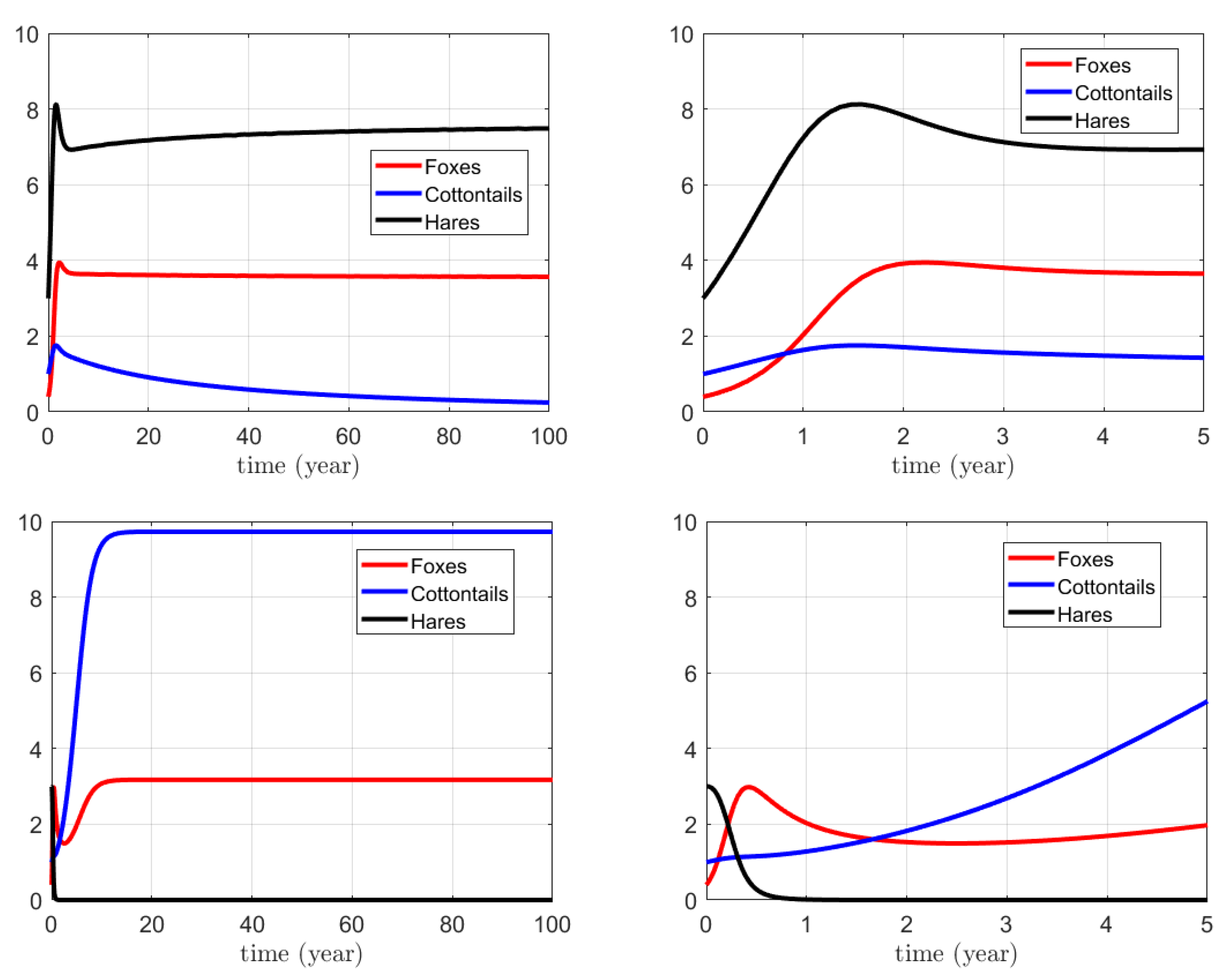
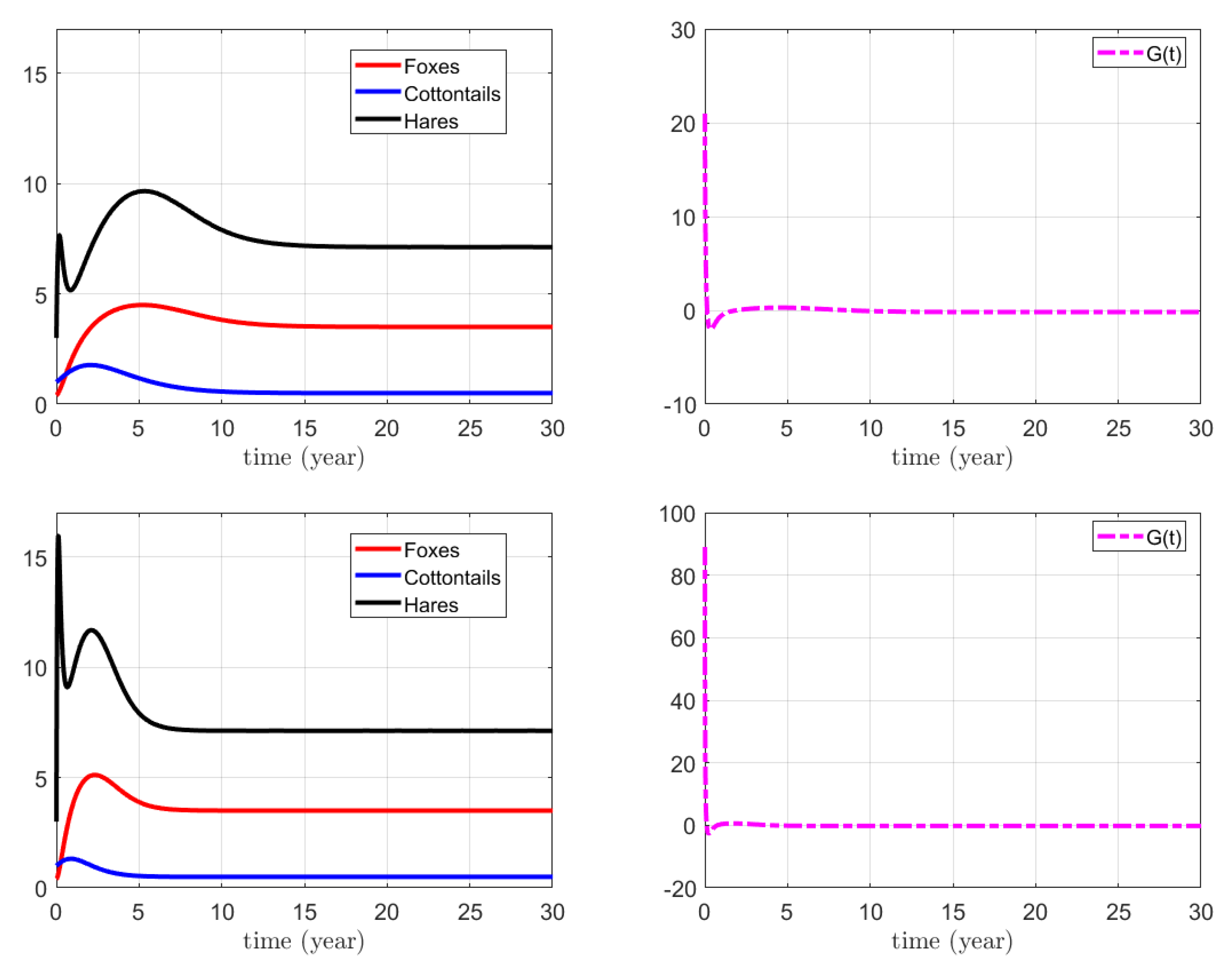
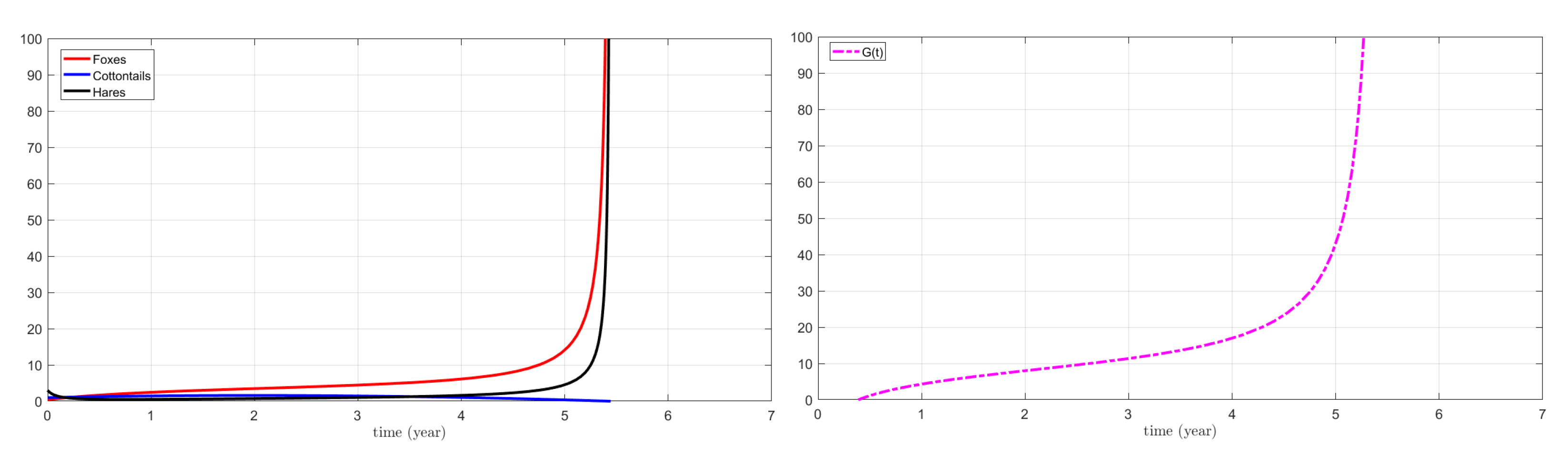
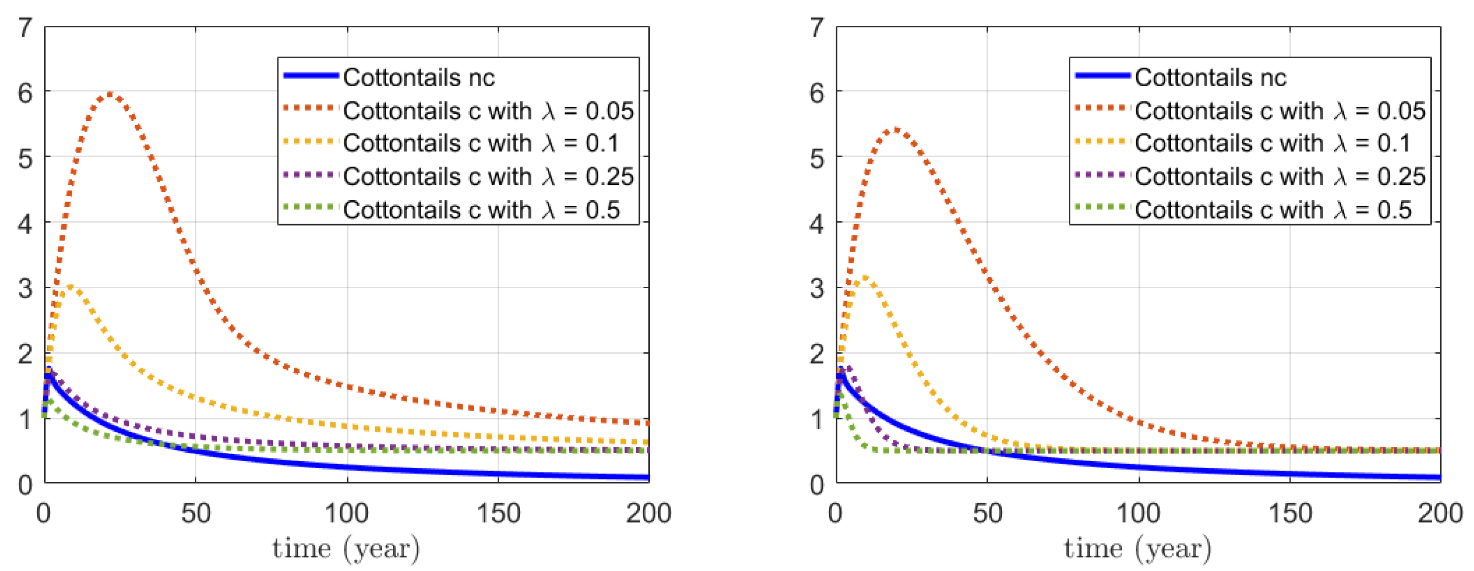
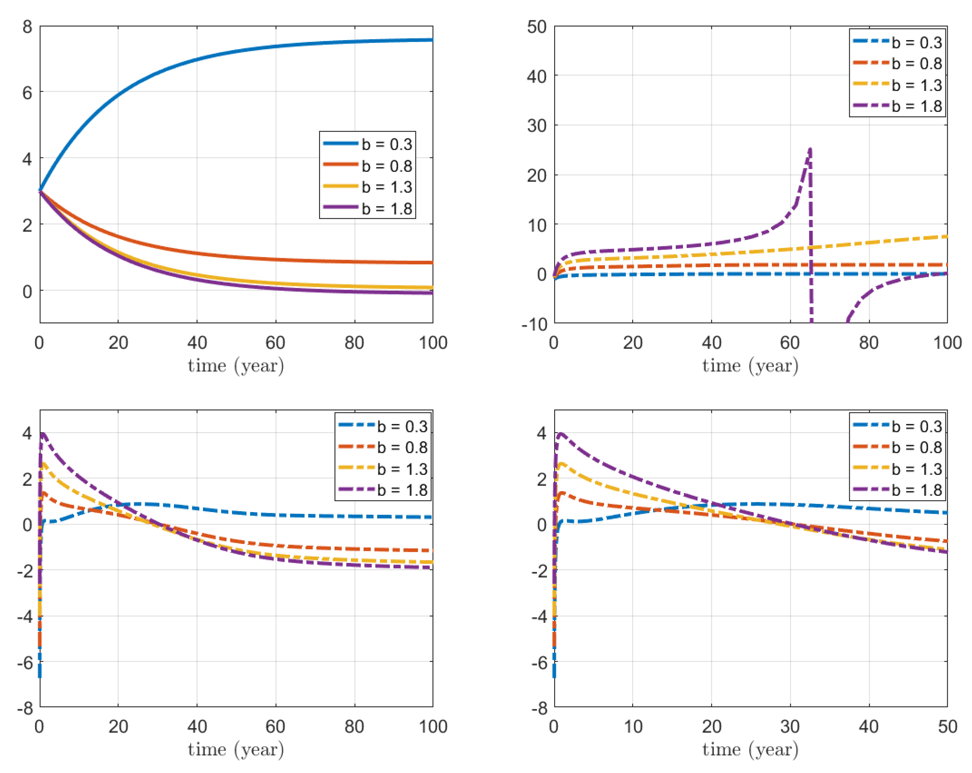
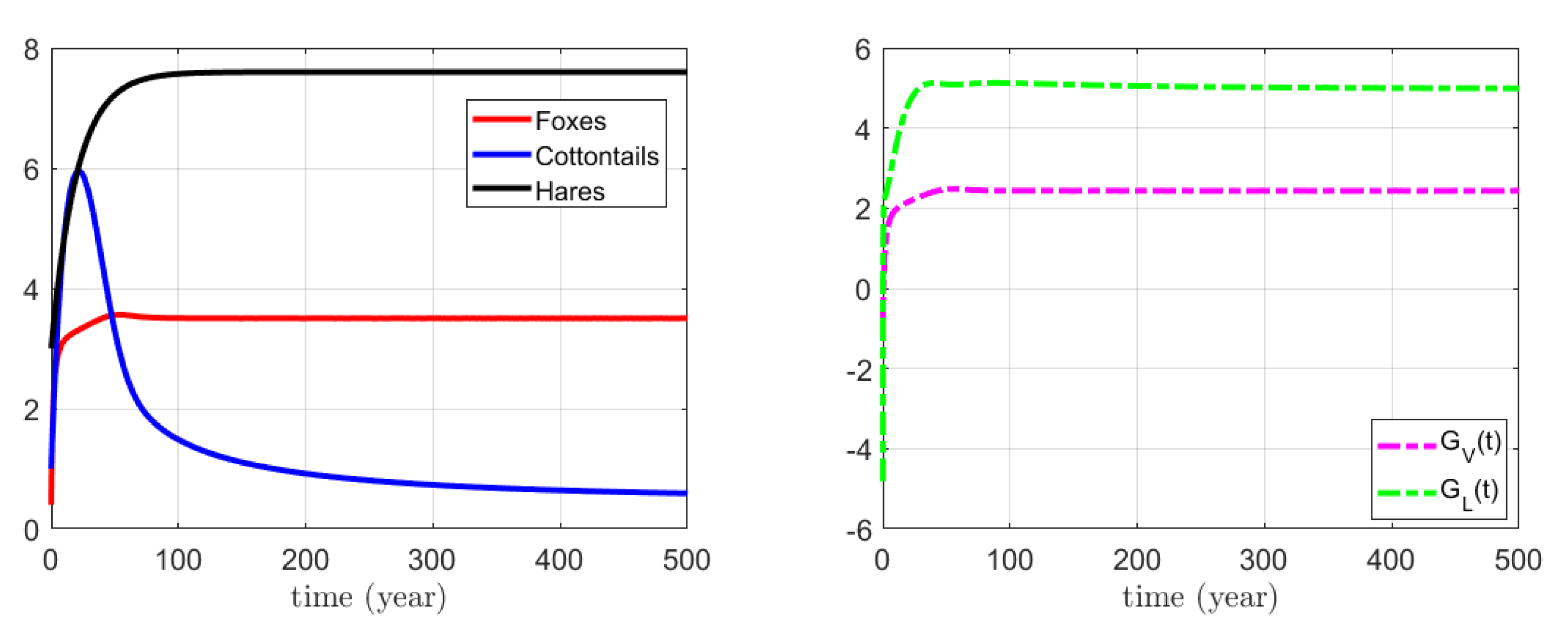
3.1. Numerical Simulations for the Action on Foxes

Suppose we want to reduce the invasive population to a lower value, so that $S_d$ is set to, say, $0.5$. We distinguish two cases for the choice of the parameter b. A low value, specifically when $b=0.3$, simulates a situation where foxes hunt the two prey almost indistinguishably, at the same rates $b\sim a$. On the contrary, the larger value $b=3$ represents a scenario of hyperpredation on hares. We observe that $b^{*}\approx 0.4076$ and therefore these two different situations could indeed occur. Figure 2 shows the model with no control, respectively, with $b=0.3$ and $b=3$. In the first case, the cottontail population naturally decreases and with this choice of parameters the equilibrium $E_5$ of the uncontrolled reference model (2) is feasible and locally stable. The equilibrium values for the native species are, respectively,

$$V_5\approx 3.5529\mathrm{and}{L}_5\approx 7.6017$$

(27)

and these levels are reached relatively soon, after about 3 years. This scenario would not require an excessive control, as the invasive species naturally tends to disappear. However, we discuss how the application of Z-control can affect this process and which scenario may be more advantageous. Figure 3 and Figure 4 show the population behavior in the controlled model with $b=0.3$, as well as the control function $G_{\mathrm{pred}}\left(t\right)$ with $\lambda =0.01$, $\lambda =0.025$, $\lambda =0.05$, $\lambda =0.1$ and $\lambda =0.7$, respectively. We observe that, since b is low, a control with a small $\lambda$, for example $\lambda =0.01$ or $\lambda =0.025$, should already produce a good result. In this case, however, a weak control initially produces an increase in the cottontail population and thus slows down the natural process for cottontails’ extinction, so its employment does not add any advantages. Additional forcing means a higher convergence speed to the desired state, as expected from a theoretical point of view, and a gradual lowering of the cottontails’ curve. Furthermore, we observe that when a faster convergence is required, as in the case of $\lambda =0.1$, the control function $G_{\mathrm{pred}}\left(t\right)$ indicates that a considerably high effort is necessary in order to guide the populations towards the configuration $E_c$. The stable equilibrium of the controlled model is $E_c=(3.5028,0.5,7.9177)$; comparing these values with those of $E_5$, compare (27), we observe that the control does not result in a significantly better situation than the uncontrolled one.

Focusing now on the second scenario, represented in Figure 5 and Figure 6, we observe that in the uncontrolled model ($b=3$), the cottontails’ invasion leads to the extinction of the native prey L and the local feasibility and stability conditions for equilibrium $E_3=(3.1779,9.7277,0)$, where the predator and invasive species coexist, are satisfied. In this situation, the Z-control action plays a crucial role to eradicate the invasive species but it is not sufficient to ensure the survival of hares since, with $b>b^{*}$, the only admissible stationary configuration is represented by $E_L=(3.5028,0.5,0)$. In particular, $E_L$ is locally asymptotically stable. As in the previous case, as the value of $\lambda$ increases, the convergence of S to $S_d$ strengthens, and the effort employed by $G_{\mathrm{pred}}\left(t\right)$ increases as well.

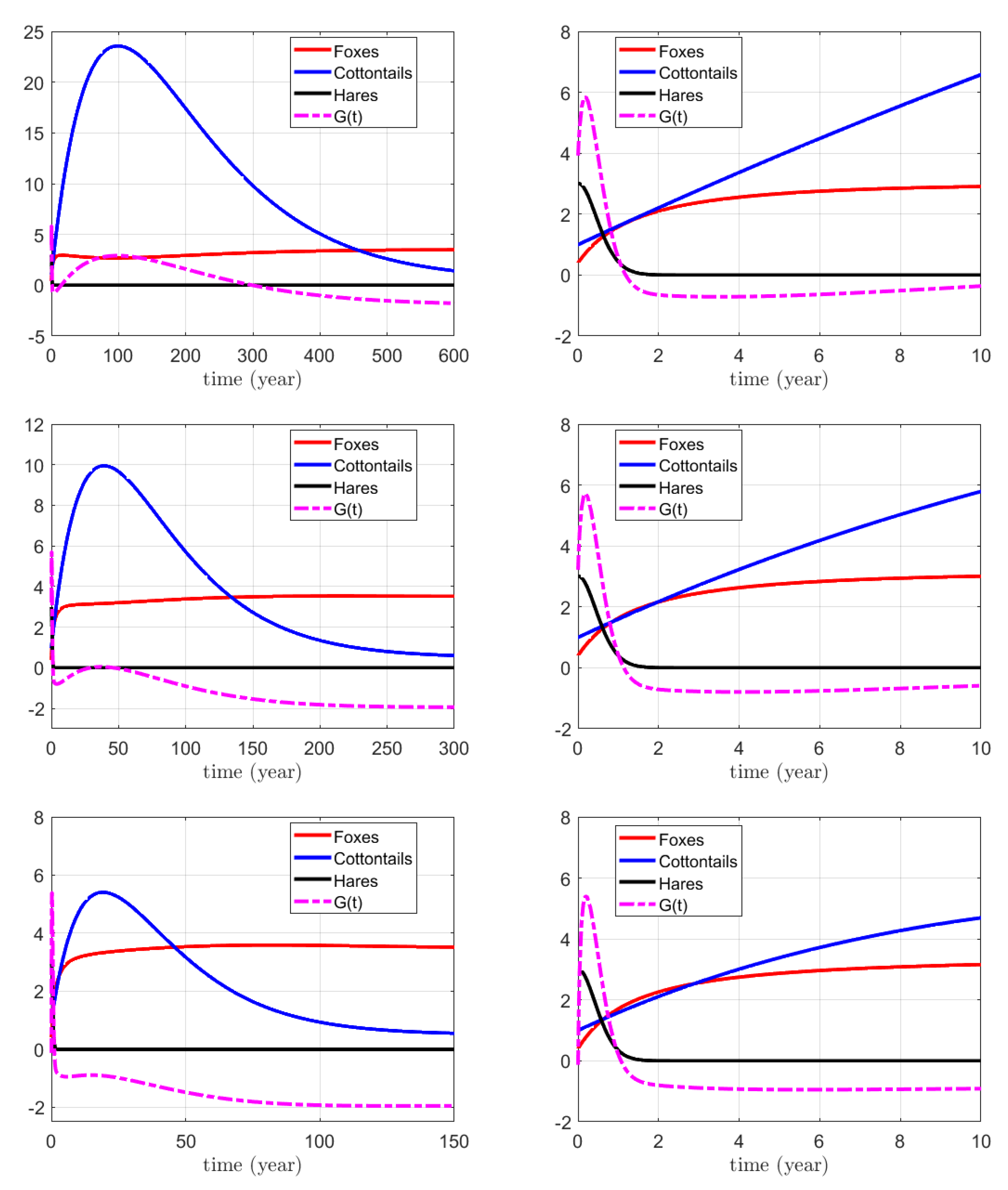
3.2. Numerical Simulations for the Action on Hares

We now discuss the second approach (16) employed for reducing the invasive species, where the desired state is assumed to be $S_d=0.5$. For this model, the equilibrium $\tilde{E}=(3.5028,S_d,\tilde{L})$ is always feasible with the choice made on parameters, but its local stability depends on the $\lambda$ values. We also observe that the hares value $\tilde{L}$ at the equilibrium depends on b: according to (17), it is inversely proportional to the hunting parameter. In order to investigate the stability conditions (18) for this situation, we can graphically observe in Figure 7 that $\tilde{D}<0$, i.e., $-{\lambda }^3+(c_{VV}\tilde{V}+c_{SS}{S}_d-3\lambda )(c_{VV}+ea)\left(a{S}_d\right)\tilde{V}<0$, if $\lambda >0.6668$. Moreover, the numerical real solution resulting from the intersection of the cubic polynomials $3\lambda \tilde{B}\left(\lambda \right)$ and $\tilde{D}\left(\lambda \right)$ involved in (18), i.e., the real solution of

$$3\lambda [\left(c_{VV}\tilde{V}\right)\left(c_{SS}{S}_d\right)-3{\lambda }^2]=-{\lambda }^3+(c_{VV}\tilde{V}+c_{SS}{S}_d-3\lambda )(c_{VV}+ea)\left(a{S}_d\right)\tilde{V},$$

is $\lambda =-0.5879$ (Figure 7). Therefore, local stability for $\tilde{E}$ is guaranteed if $\lambda >0.6668$ and does not depend on the choice of b. In line with the previous section, we perform simulations to explore the system’s behavior which may lead to instability scenarios, across a range of values for $\lambda$ together with the two previously used values of b.

Figure 8 and Figure 9 show the controlled model with $\lambda =0.7$ and $\lambda =1.4$, both for $b=0.3$ and $b=3$, where the values for $\tilde{L}$ are ${\tilde{L}}_{\left(0.3\right)}\approx 7.1191$ and ${\tilde{L}}_{\left(3\right)}\approx 0.7119$, respectively. In these situations, the convergence speed to the equilibrium is quite high and, once again, it increases for higher values of $\lambda$.

To observe a different situation, let us consider, for example, the case where $b=3$ and $\lambda =0.025$, illustrated in Figure 10: the control function in the bottom panel is unbounded and, after approximately 5 years, the introduction of hares into the territory grows indefinitely, therefore influencing the native population’s behavior. This fact could be interpreted as a restoration of the coexistence of native species, as the growth is attributed to a continuous introduction of prey into the territory. Indeed, the cottontail population decrease with time, leading to extinction.

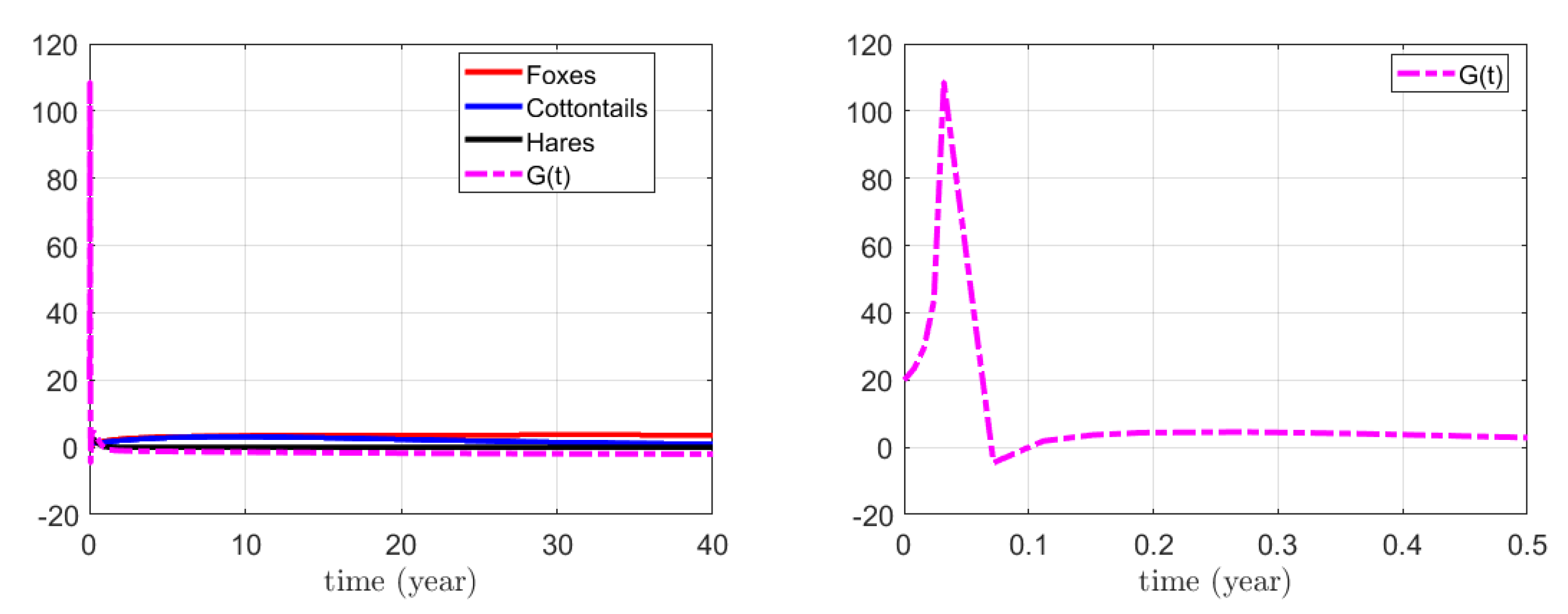
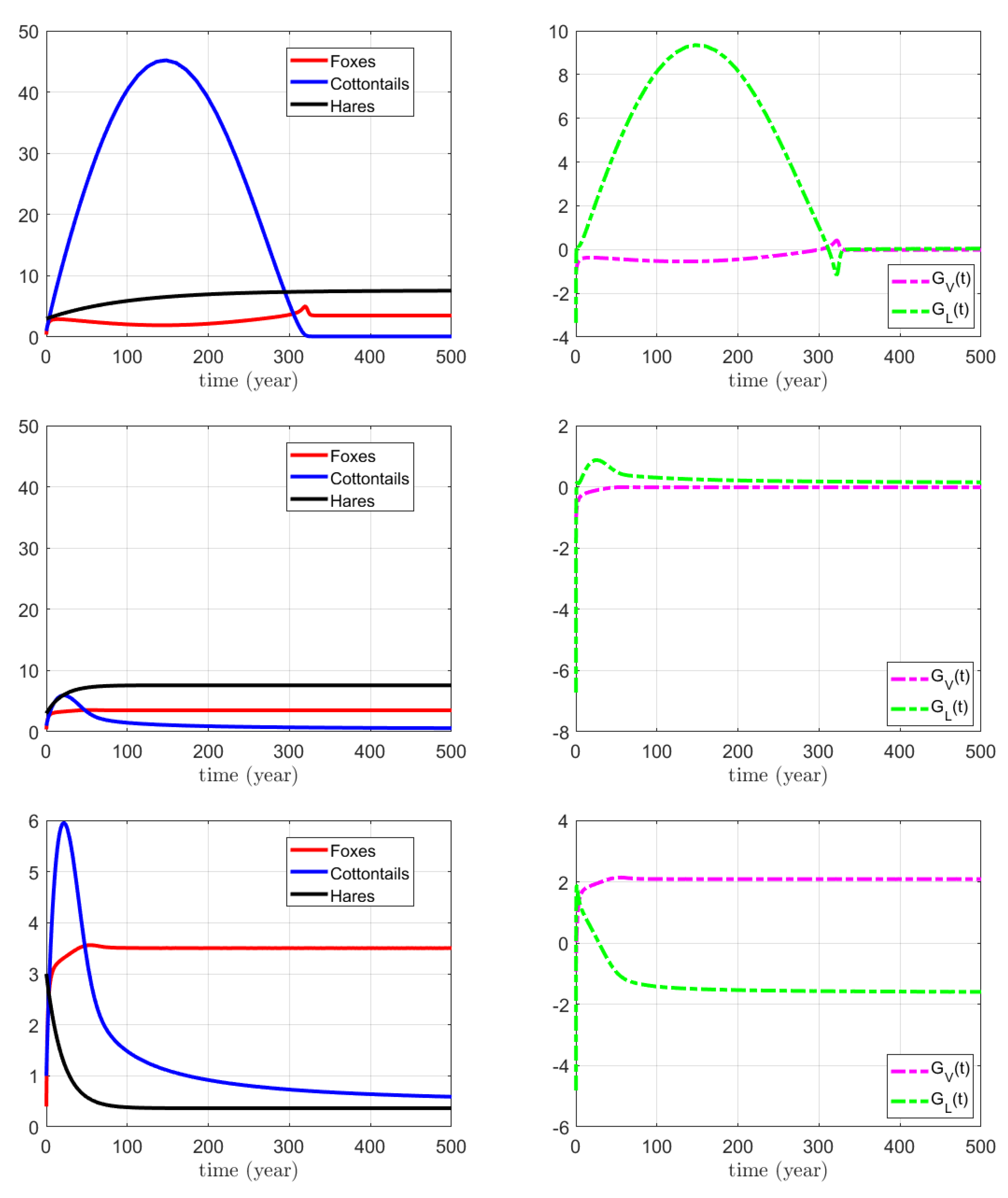
3.3. Numerical Simulations for the Combined Action on Foxes and Hares

We finally consider the model (22) with action on both foxes and hares choosing as desired states the values $S_d=0.5$ and $L_d=L_5$, as first trial. We will then discuss the case $L_d<K_{\left(L\right)}$ and compare which choice may be better. For this controlled model, the equilibrium is $E_c^{*}=(3.5028,S_d,L_d)$. We observe that $L_5$, whose expression is presented again in the next equation, depends on the choice of b and in particular its value decreases as b increases (assuming the other parameters are fixed)

$$L_5={\displaystyle \frac{b(m-r)+c_{VV}(u-p)}{b^{2}e+c_{VV}{c}_{LL}}}.$$

Therefore, in order to have a feasible equilibrium, b has to be chosen so that

$$b<-{\displaystyle \frac{c_{VV}(u-p)}{m-r}}\approx 1.4276$$

(28)

and, furthermore, if b is larger than a certain threshold, the use of this method could drive the class L towards a desired state $L_5$ that could represent extinction. Figure 11 shows the simulations in the case in which (28) is satisfied, particularly with $b=0.3$ (for different values of $\lambda$) and $b=1$. In these two cases, $L_5=7.6017$ and $L_5=0.3664$, respectively.

From Figure 11, we observe that an increase in the value of $\lambda$ leads to a faster convergence. In this case, we also note that, as this parameter increases, the need for adding hares becomes lower and lower and consequently this is reflected in the decreasing of the function $G_L\left(t\right)$. This fact can be explained by observing that higher values of $\lambda$ better reflect the natural undisturbed system behavior. Instead, lower ones impose a convergence speed slower than the one which is naturally exhibited; counterintuitively, it produces a general slowdown of the convergence process. This point is also apparent in the sequence of panels of Figure 3. On the other hand, it appears that above a certain threshold, the system is forced to converge at a faster rate than its natural behavior, resulting in greater external effort. Figure 12 shows the changes in the cottontails’ curve for different values of $\lambda$ in the case of the controlled model with action on foxes (left panel) compared to the double action on V and L (right panel). In particular, smaller values of $\lambda$ show a peak in the cottontail population, which decreases with the increase in this parameter and thus better approaches the natural trajectory. However, for early times, the best situation appears to be given by an intermediate value, such as $\lambda =0.25$.

As observed in previous cases, in the uncontrolled system with $b=0.3$, the invasive species naturally goes extinct, and the dual action through the Z-control works from a mathematical perspective but is not necessary in practice. On the other hand, by increasing b, e.g., $b=1$, the class L is indeed driven towards a lower value (for instance $L_5=0.3664$). If b does not satisfy (28), hares are driven to extinction because $L_5$ turns out to be negative. Figure 13 shows the behavior of the class L and the control functions for b varying between $0.3$ and $1.8$.

To conclude this section, the case $L_d<K_{\left(L\right)}$ is considered. For example, set $L_d$ approximately equal to the value achieved at the equilibrium configuration $E_5$ when $b=0.3$ as calculated in (27), so $L_d=7.6$. An instance of this situation is presented in Figure 14.

4. Discussion

4.1. Biological Interpretation for Indirect Control on Foxes

For the first model, external intervention is made through predator removal or reintroduction into the territory. Numerical results enable us to primarily compare two distinct situations. For the first one, where $b=0.3$, one may expect that the application of Z-control speeds up the process of extinction of the cottontails. This is possible from a theoretical point of view, since the cottontails’ class converges to the desired state, but it may be resource-demanding from a practical perspective. For instance, the first row of Figure 4 illustrates that around half a month after the invasion, the number of individuals to be removed or relocated exceeds 100. Moreover, the values attained at the equilibrium reflect the scenario that would naturally occur without any intervention. As a further example, looking at the second row of Figure 4, we observe in the graph of $G_{\mathrm{pred}}$ that predator insertion and removal should alternate, presenting a more practical approach. However, non-intervention might be preferable.

On the other hand, the second scenario, where $b=3$, represents an invasive phenomenon where the invasive species settles in the territory, negatively affecting the survival of the native prey. Unlike the previous case, here both prey populations go extinct. Hence, the natural pre-invasion dynamics between native species are disrupted and predators may be forced to seek new resources elsewhere.

4.2. Biological Interpretation for Indirect Control on Hares

Among the two methods indirectly applied to control the cottontails’ curve, the second one may yield better results. In this situation, the behavior of the function $G_{\mathrm{prey}}$ represents the introduction or removal of native hares, depending on its sign. From an analysis of Figure 8, Figure 9 and Figure 10, we can observe that, in addition to the removal of the invasive species, the survival of hares can also be assured without being imposed. Furthermore, even for those values of $\lambda$ that do not make the unique equilibrium locally stable, situations of coexistence among the native species can still be achieved. Hence, a restoration of the dynamic interaction between foxes and hares becomes feasible for these simulations.

4.3. Biological Interpretation for Combined Indirect Control on Foxes and Hares

By combining the previous approaches, it becomes possible to impose two conditions to ensure both the removal of the invasive prey and the survival of the native one. In principle, this technique is expected to be more resource-intensive since it involves two parallel efforts. However, it may also be more effective, as the controlled classes converge to the desired states. Specifically, forcing the hares’ population towards a level $L_d$, it is possible to achieve favorable outcomes with control functions that do not entail excessive effort, as shown in Figure 11. Therefore, this method can provide, for the situation examined in this work, a balanced strategy to address the invasion issue of the pre-existing ecosystem.

5. Conclusions

In this paper, the Z-type control method was applied in an ecological context involving a native predator, the fox, and two preys, one native and one invasive, hares and cottontails, respectively. Our goal was to explore some situations in which the invasive species could be kept at low values while preserving the critically endangered native prey, in order to possibly give indications to ecosystem managers. Specifically, we considered three possible alternatives to act on the ecosystem. At first, we considered predator removal in order to curb the invasive cottontails causing the hyperpredation effect on hares. We applied an indirect control on the cottontails acting on foxes to reduce the pressure on hares. Then, we considered the possibility of importing new individuals of the indigenous prey population from outside, employing a direct control on this class. This choice sustains the hare population although it also provides more resources for foxes. However, this may entail other problems due to the emergence of hybrid species, a problem addressed in [31]. Finally, we combined the two strategies initially proposed: direct control on hares and indirect control on the cottontails acting on foxes. In the first case, the controlled model can evolve toward two equilibrium points, coexistence and hare-free equilibrium. Both are found to be conditionally admissible and locally asymptotically stable. Moreover, a transition from one to the other is possible through a transcritical bifurcation as the value of the hunting rate of foxes on hares varies. In the last two cases, instead, the controlled system can only converge to a conditionally admissible and stable coexistence equilibrium. Consequently, with a view to preserving the hare population, we can conclude that the best solutions among the three proposed to manage the cottontail invasion problem would seem to be the last two. Indeed, by applying indirect control on cottontails acting on foxes, the hare-free equilibrium may arise, entailing the hares’ extinction. This cannot happen in the remaining two cases because the corresponding controlled models can only evolve toward the coexistence of the three populations involved, where the cottontail population can be kept as small as desired. In this regard, however, we stress that choosing either of the last two proposed strategies could give rise to other secondary problems. Considering the numerical results, comparisons between the three models and the original unmodified one have been made. Specifically, the attention was focused on different scenarios relying on the choice of the parameter b. The situations in which it was assumed that hares are hunted at rate $b=3$, approximately 10 times higher than the value chosen for a, may be more interesting and significant from a biological point of view. Instead, the case in which b was kept lower, e.g., $b=0.3$, could be more interesting from a theoretical perspective, since the system naturally evolves to the desired state. For the specific situation where $b=3$, our conclusions indicate that it is not necessary to apply the Z-control method, mainly for two reasons. On one hand, the cottontails’ curve undergoes a significant slowdown in the convergence to zero, since the choice of $\lambda$ greatly affects the dynamics of the system; on the other one, in some cases, requiring higher convergence speed to the desired solution involves a great effort that could become not practicable. In conclusion, our goal was primarily to show that the method is at least theoretically viable, a task that has been achieved, and to explore different ways of implementing the Z-control approach in a real-world scenario.

References

1. Pyšek, P.; Hulme, P.E.; Simberloff, D.; Bacher, S.; Blackburn, T.M.; Carlton, J.T.; Dawson, W.; Essl, F.; Foxcroft, L.C.; Genovesi, P.; et al. Scientists’ warning on invasive alien species. Biol. Rev. 2020, 95, 1511–1534. [Google Scholar] [CrossRef] [PubMed]
2. Bellavere, E.; Venturino, E. Crossing the desert: A model for alien species invasion containment or to lessen habitat disruption effects. J. Biol. Syst. 2023, 31, 557–589. [Google Scholar] [CrossRef]
3. Harms, W.B.; Stortelder, A.H.F.; Vos, W. Effects of intensification of agriculture on nature and landscape in the Netherlands. In Land Transformation in Agriculture; Wolman, M.G., Fournier, F.G.A., Eds.; SCOPE Publication 32; John Wiley: New York, NY, USA, 1987; pp. 357–380. [Google Scholar]
4. Huffaker, C.B.; Kennett, C.E.; Finney, G.L. Biological control of olive scale. Parlatoria oleae in California by imported Aphytis maculiformis (Hymenoptera; Aphelinidae). Hilgardia 1962, 32, 541–636. [Google Scholar] [CrossRef]
5. Isaia, M.; Bona, F.; Badino, G. Influence of landscape diversity and agricultural practices on spiders assemblage in Italian vineyards of Langa Astigiana (Northwest Italy). Environ. Entomol. 2006, 35, 297–307. [Google Scholar] [CrossRef]
6. Brown, K.C.; Lawton, J.H.; Shires, S. Effects of insecticides on invertebrate predators and their cereal aphid (Hemiptera: Aphidae) prey: Laboratory experiments. Environ. Entomol. 1983, 12, 1747–1750. [Google Scholar] [CrossRef]
7. Nyffeler, M.; Benz, G. Spiders in natural pest control: A review. J. Appl. Entomol. 1987, 103, 321–339. [Google Scholar] [CrossRef]
8. Sunderland, K.D.; Samu, F. Effects of agricultural diversification on the abundance, distribution, and pest control potential of spiders: A review. Entomol. Exp. Appl. 2000, 95, 113. [Google Scholar] [CrossRef]
9. Wise, D.H. Spiders in Ecological Webs; Cambridge University Press: London, UK, 1993. [Google Scholar]
10. DeBach, P.; Rosen, D. Biological Control by Natural Enemies; Cambridge University Press: London, UK, 1991. [Google Scholar]
11. Flaherty, D.L.; Huffaker, C.B. Biological control of pacific mites and Willamette mites in San Joaquin Valley vineyards, I. Role of Metaseilus occidentalis. Hilgardia 1970, 40, 267–308. [Google Scholar] [CrossRef]
12. Marc, P.; Canard, A. Maintaining spider biodiversity in agroecosystems as a tool in pest control. Agric. Ecosyst. Environ. 1997, 62, 229–235. [Google Scholar] [CrossRef]
13. Marc, P.; Canard, A.; Ysnel, F. Spiders (Aranee) useful for pest limitation and bioindication. Agric. Ecosyst. Environ. 1999, 74, 229–273. [Google Scholar] [CrossRef]
14. Wood, B.J. Development of integrated control programs for pests of tropical perennial crops in Malaysia. In Biological Control; Huffaker, C.B., Ed.; Plenum Press: New York, NY, USA, 1971; pp. 423–457. [Google Scholar]
15. Pappalardo, S.; Villa, M.; Santos, S.A.P.; Benhadi-Marín, J.; Pereira, J.A.; Venturino, E. A tritrophic interaction model for an olive tree pest, the olive moth Prays oleae (Bernard). Ecol. Model. 2021, 462, 10977. [Google Scholar] [CrossRef]
16. Simberloff, D.; Martin, J.L.; Genovesi, P.; Maris, V.; Wardle, D.A.; Aronson, J.; Courchamp, F.; Galil, B.; García-Berthou, E.; Pascal, M.; et al. Impacts of biological invasions: What’s what and the way forward. Trends Ecol. Evol. 2013, 28, 58–66. [Google Scholar] [CrossRef] [PubMed]
17. Clavero, M.; García-Berthou, E. Invasive species are a leading cause of animal extinctions. Trends Ecol. Evol. 2005, 20, 110. [Google Scholar] [CrossRef] [PubMed]
18. Rilov, G. Predator-Prey Interactions of Marine Invaders. In Biological Invasions in Marine Ecosystems: Ecological, Management, and Geographic Perspectives; Springer: Berlin/Heidelberg, Germany, 2009; pp. 261–285. [Google Scholar] [CrossRef]
19. Norbury, G. Conserving dryland lizards by reducing predator-mediated apparent com- petition and direct competition with introduced rabbits. J. Appl. Ecol. 2001, 38, 1350–1361. [Google Scholar] [CrossRef]
20. Bertolino, S.; Perrone, A.; Gola, L.; Viterbi, R. Population density and habitat use of the introduced Eastern Cottontail (Sylvilagus floridanus) compared to the native European Hare (Lepus europaeus). Zool. Stud. 2011, 50, 315–326. [Google Scholar]
21. Bertolino, S.; di Montezemolo, N.C.; Perrone, A. Daytime habitat selection by introduced Eastern Cottontail Sylvilagus floridanus and native European hare Lepus Europaeus in Northern Italy. Zool. Sci. 2011, 28, 414–419. [Google Scholar] [CrossRef] [PubMed]
22. Bertolino, S.; di Montezemolo, N.C.; Perrone, A. Habitat use of coexisting introduced eastern cottontail and native European hare. Mamm. Biol. 2013, 78, 235–240. [Google Scholar] [CrossRef]
23. Cerri, J.; Ferretti, M.; Bertolino, S. Rabbits killing hares: An invasive mammal modifies native predator-prey dynamics. Anim. Conserv. 2017, 20, 511–519. [Google Scholar] [CrossRef]
24. Caudera, E.; Viale, S.; Bertolino, S.; Cerri, J.; Venturino, E. A mathematical model supporting a hyperpredation effect in the apparent competition between invasive Eastern cottontail and native European hare. Bull. Math. Biol. 2021, 83, 51. [Google Scholar] [CrossRef]
25. Laticignola, D.; Diele, F. On the Z-type control of backward bifurcations in epidemic models. Math. Biosci. 2019, 315, 108215. [Google Scholar]
26. Laticignola, D.; Diele, F. Using awareness to Z-control a SEIR model with overexposure: Insights od Covid-19 pandemic. Chaos Solitons Fractals 2021, 150, 111063. [Google Scholar] [CrossRef]
27. Laticignola, D.; Diele, F.; Marangi, C.; Provenzale, A. On the dynamics of a generalized predator-prey system with Z-type control. Math. Biosci. 2016, 280, 10–23. [Google Scholar] [CrossRef]
28. Zhang, Y.; Yan, X.; Liao, B.; Zhang, Y.; Ding, Y. Z-type control of populations for Lotka-Volterra model with exponencial convergence. Math. Biosci. 2016, 272, 15–23. [Google Scholar] [CrossRef]
29. Zhang, Z.; Zhang, Y. Design and experimentation of acceleration-level drift-free scheme aided by two recurrent neural networks. IET Control Theory Appl. 2013, 7, 25–42. [Google Scholar] [CrossRef]
30. Perko, L. Differential Equations and Dynamical Systems; Springer: New York, NY, USA, 2001. [Google Scholar]
31. La Morgia, V.; Venturino, E. Understanding hybridization and competition processes between hare species: Implications for conservation and management on the basis of a mathematical model. Ecol. Model. 2017, 364, 13–24. [Google Scholar] [CrossRef]
32. Pandini, W.; Tosi, G.; Meriggi, A.; Lepre, L.; Bianca, C.; Selvatico, S.; Simonetta, A.M.; Dessì-Fulgheri, F. Principi e tecniche di gestione faunistico-venatoria. Greentime 1998, 195–220. [Google Scholar]
Figure 1. Transcritical bifurcation from E c to E L at b = b * 0.4076 , with S d = 0.5 and λ = 0.01 . The initial conditions are in (14) and the ecological parameter values are in (15). (Left) panel: b = 0:0.025:1. (Right) panel: zoom with b = 0.38:0.0015:0.44.
Mathematics 11 04182 g001
Figure 2. (Left): Population behavior for the uncontrolled Model (2) with b = 0.3 (top) or b = 3 (bottom). (Right): zoom of the left panels near the origin.
Mathematics 11 04182 g002
Figure 3. (Left): Population behavior and control function G pred ( t ) for parameters b = 0.3 and λ = 0.01 (top), λ = 0.025 (middle) or λ = 0.05 (bottom). (Right): zoom of the left panels near the origin.
Mathematics 11 04182 g003
Figure 4. (Left): Population behavior and control function G pred ( t ) for parameters b = 0.3 and λ = 0.1 (top) or λ = 0.7 (bottom). (Right): zoom of the control functions near the origin.
Mathematics 11 04182 g004
Figure 5. (Left): Population behavior and control function G pred ( t ) for parameters b = 3 and λ = 0.01 (top), λ = 0.025 (middle) or λ = 0.05 (bottom). (Right): zoom of the left panels near the origin.
Mathematics 11 04182 g005
Figure 6. (Left): Population behavior and control function G pred ( t ) for parameters b = 3 and λ = 0.1 . (Right): zoom of the control function near the origin.
Mathematics 11 04182 g006
Figure 7. (Top, Left): Graph of D ˜ (blue line) as a cubic function of λ . (Bottom, Left): Graphs of D ˜ ( λ ) (blue line) and 3 λ B ˜ ( λ ) (orange line). (Right): zoom of the left panels.
Mathematics 11 04182 g007
Figure 8. Population behavior (left) and control function G prey ( t ) (right) over time for parameters b = 0.3 and λ = 0.7 (top) or λ = 1.4 (bottom).
Mathematics 11 04182 g008
Figure 9. Population behavior (left) and control function G prey ( t ) (right) over time for parameters b = 3 and λ = 0.7 (top) or λ = 1.4 (bottom).
Mathematics 11 04182 g009
Figure 10. Population behavior (left) and control function G prey ( t ) (right) as function of time for parameters b = 3 and λ = 0.025 .
Mathematics 11 04182 g010
Figure 11. Population behavior ((left) panels) and the control functions G V ( t ) and G L ( t ) ((right) panels, respectively, in magenta and green) over time for parameters b = 0.3 and λ = 0.01 (top), b = 0.3 and λ = 0.05 (middle), b = 1 and λ = 0.05 (bottom).
Mathematics 11 04182 g011
Figure 12. Comparison between the cottontails’ curve of the uncontrolled Model (2) for b = 0.3 (continuous line identified with nc in the legend) and the controlled models with single action on foxes (Model (3), (left) panel) and action on foxes and hares (Model (22), (right) panel) for different values of λ .
Mathematics 11 04182 g012
Figure 13. Class L ((top left) panel) and control functions G L ( t ) ((top right) panel) and G V ( t ) ((bottom left) panel, with zoom in the (bottom right) one) behavior for b = 0.3 : 0.5: 1.8 and λ = 0.05 .
Mathematics 11 04182 g013
Figure 14. Population behavior ((left) panel) and control functions G V ( t ) and G L ( t ) ((right) panel, respectively, in magenta and green) as a function of time for parameters b = 1 and λ = 0.05 .
Mathematics 11 04182 g014
Disclaimer/Publisher’s Note: The statements, opinions and data contained in all publications are solely those of the individual author(s) and contributor(s) and not of MDPI and/or the editor(s). MDPI and/or the editor(s) disclaim responsibility for any injury to people or property resulting from any ideas, methods, instructions or products referred to in the content.