Utilizing m-Polar Fuzzy Saturation Graphs for Optimized Allocation Problem Solutions

Abstract

It is well known that crisp graph theory is saturated. However, saturation in a fuzzy environment has only lately been created and extensively researched. It is necessary to consider m components for each node and edge in an m-polar fuzzy graph. Since there is only one component for this idea, we are unable to manage this kind of circumstance using the fuzzy model since we take into account m components for each node as well as edges. Again, since each edge or node only has two components, we are unable to apply a bipolar or intuitionistic fuzzy graph model. In contrast to other fuzzy models, mPFG models produce outcomes of fuzziness that are more effective. Additionally, we develop and analyze these kinds of mPFGs using examples and related theorems. Considering all those things together, we define saturation for a m-polar fuzzy graph (mPFG) with multiple membership values for both vertices and edges; thus, a novel approach is required. In this context, we present a novel method for defining saturation in mPFG involving m saturations for each element in the membership value array of a vertex. This explains $\alpha$-saturation and $\beta$-saturation. We investigate intriguing properties such as $\alpha$-vertex count and $\beta$-vertex count and establish upper bounds for particular instances of mPFGs. Using the concept of $\alpha$-saturation and $\alpha$-saturation, block and bridge of mPFG are characterized. To identify the $\alpha$-saturation and $\beta$-saturation mPFGs, two algorithms are designed and, using these algorithms, the saturated mPFG is determined. The time complexity of these algorithms is $O\left(\right|V{|}^3)$, where $\left|V\right|$ is the number of vertices of the given graph. In addition, we demonstrate a practical application where the concept of saturation in mPFG is applicable. In this application, an appropriate location is determined for the allocation of a facility point.

1. Introduction

Graph theory is a powerful mathematical framework used to model relationships and connections among objects. In many real-world applications, it is essential to understand the strength or degree of association between various elements within a graph. Saturation is a concept that plays a crucial role in quantifying this degree of connection and is particularly significant in both traditional graphs and fuzzy graphs.

In traditional graph theory, saturation refers to the level of connectivity or completeness within a graph. More formally, the saturation of a vertex in a graph is a measure of how many edges are incident upon that vertex concerning the total possible number of edges it could have. In simpler terms, it tells us how closely a particular vertex is connected to others in the graph.

1.1. Research Background and Related Work

Fuzzy graph theory extends the traditional graph theory to capture uncertainty and imprecision in relationships. In fuzzy graphs, saturation takes on a more nuanced meaning. Instead of sharp connectivity values (0 or 1), vertices in fuzzy graphs are associated with degrees of membership that represent the strength of connections.

Saturation in fuzzy graphs involves quantifying the degree to which a vertex is related to other vertices in a fuzzy and uncertain context. It allows us to express the level of association between vertices as fuzzy values, which can be continuous and gradual. This approach is particularly valuable in situations where the connections between elements are not binary but exhibit varying degrees of affinity.

Applications of saturation in fuzzy graphs can be found in fields such as decision-making, pattern recognition, image processing, and artificial intelligence, where imprecise information needs to be modelled and analyzed.

In both traditional and fuzzy graphs, the concept of saturation offers valuable insights into the structure and dynamics of networks and relationships. Whether dealing with crisp, well-defined connections in traditional graphs or handling uncertainty and fuzziness in fuzzy graphs, saturation provides a quantitative measure for characterizing the strength and extent of associations, enabling more informed decision-making and analysis in various domains.

Zadeh [1], in 1965, discovered the ambiguity of the real-life situation and the phenomenon of uncertainty and introduced a fuzzy set that changed how science and technology were portrayed. Zhang [2] explained the bipolar fuzzy set idea as well as presented the possibility of bipolar fuzzy sets in different environmental analyses [3]. First, Kaufman [4] studied the fuzzy graph concept. After that, Rosenfeld [5] supplied the possibility of nodes and edges along with several theoretical ideas such as paths, connectedness, cycle, etc., in fuzziness. Different concepts are presented after that on fuzzy graphs [6]. Several definitions and real-life applications have been studied in [7]. Some new concepts of the fuzzy graph and their generalization are also discussed by Mordeson and Mathew [8]. Nair and Cheng [9] provided fuzzy graphs with fuzzy cliques. Saturation on the fuzzy graph is presented first by Mathew et al. [10]. Chen et al. [11] first presented mPFG. Later on, Ghorai and Pal [12] first introduced density on mPFG. Akram et al. [13,14] studied on a few edge properties of mPFG. Next, Mahapatra et al. [15] studied fuzzy fractional colouring on fuzzy graphs. They also discussed the threshold graph on mPF environment [16]. They also initiated the mPF tolerance graph [17]. Mandal et al. [18] studied the application of strong arcs on mPFG. They also worked on different types of arcs on mPFG [19]. Subrahmanyam [20] also introduced different types of products on mPFG. Several works on fuzzy graphs and their generalization were developed by Nagoorgani et al. [21,22,23,24]. For more terminology on fuzzy graphs and its generalized concept, one can see [25,26,27,28,29,30].

1.2. Framework of This Study

This paper is structured as follows: Section 2 describes some useful definitions in these manuscripts. In Section 3, we have discussed the definitions of the strong node as well as strong edge (SE) count, $\alpha$-node as well as $\alpha$-edge count, $\beta$-node as well as $\beta$-edge count of mPFG and give the lower and upper bound of them in an mPFG. In Section 3.1, we investigate node and edge counts of some well-known mPFG. In Section 4, we introduced saturation in mPFG with the help of $\alpha$-saturation and $\beta$-saturation. Section 5 describes algorithms used to find $\alpha$-saturated and $\beta$-saturated mPFG. Here, we also developed saturation in mPFG. Saturation in mPFG has been used to resolve an application in real life based on an allocation problem, which has been given in Section 6. Finally, a conclusion has been made in Section 7.

1.3. Motivation of the Work

Many issues in daily life have been resolved utilising data from various sources or origins. The multi-polarity of this data collection is represented. We might not be well structured in this sort of polarity by the concepts of fuzzy models or bipolar fuzzy models. For example, we consider a graph model on social groups to explain whether the group is active or not with respect to attributes of cooperation, team spirit, awareness, controlling power, good behaviour, creativeness, etc. We need to express this situation using the 3-polar fuzzy model because these terms are inherently uncertain. A fuzzy model, an intuitionistic fuzzy model, or a bipolar fuzzy model cannot be used to deal with this problem. Thus, the m-polar fuzzy model is more suitable than any fuzzy model. The development and analysis of these kinds of mPFGs with relevant instances and theorems is also quite fascinating. The previous theories about the saturation of mPFGs are unquestionably improved by these definitions and theorems, and they are more trustworthy when it comes to resolving any challenging real-world issue. If anyone considers an example to model a location problem such that there are three components of each node and edge, where the edges MV are given depending on the following criteria: {Condition of roads, traffic jams on the roads, and the communication system between two cities}. This real-life problem can be solved with the help of saturation in mPFG.

1.4. Notations and Symbols

In this section, we revise some of the significant and practical notations that are utilised throughout the whole work to establish the theories.

Table 1. Abbreviation form of some terms.

Full Name	Abbreviation Form
Fuzzy graph	FG
m-polar fuzzy graph	mPFG
Underlying crisp graph	UGC
Membership value	MV
m-polar fuzzy set	mPFS
Strength of connectedness	SC
Strong edge	SE
Maximal spanning tree	MST

provides the abbreviated forms and their meanings.

2. Preliminaries

In this section, we quickly review several terminologies related to mPFG, such as complete mPFG, strong mPFG, path in mPFG etc.

This article’s current $p_s:{[0,1]}^m\to [0,1]$ denotes $s^{th}$ projection mapping material and $s=1,2,\dots ,m$ stands for $s=1\left(1\right)m$.

Definition 1

([12]). An mPFG is denoted as $H=(\tilde{V},\sigma ,\gamma )$ over a crisp graph $H^{\ast }=(\tilde{V},\tilde{E})$, where $\tilde{V}$ and $\tilde{E}$ respectively denote the set of vertices and edges of $H^{\ast }$. The functions $\sigma :\tilde{V}\to {[0,1]}^m$ and $\gamma :\tilde{V}\times \tilde{V}\to {[0,1]}^m$ represent the membership value of vertices and edges, respectively. Also, $p_i\circ \gamma (x,t)\le p_i\circ \sigma \left(x\right)\wedge p_i\circ \sigma \left(t\right)$ for every $i=1\left(1\right)m$ and $(x,t)\in \tilde{V}\times \tilde{V}$, while $\gamma (x,t)=0$ for every $(x,t)\in (\tilde{V}\times \tilde{V}-\tilde{E})$.

Definition 2

([12]). An mPFG $H=(\tilde{V},\sigma ,\gamma )$ is called a complete mPFG if $p_s\circ \gamma (x,t)=\{p_s\circ \sigma \left(x\right)\wedge p_s\circ \sigma \left(t\right)\},$ for each $x,t\in \tilde{V}$ and $s=1\left(1\right)m$.

Definition 3

([12]). An mPFG $H=(\tilde{V},\sigma ,\gamma )$ is called an mPF strong graph if

$$p_s\circ \gamma (x,t)=\{p_s\circ \sigma \left(x\right)\wedge p_s\circ \sigma \left(t\right)\},$$

for every $(x,t)\in \tilde{E}$ and $s=1\left(1\right)m$.

Definition 4

([13]). Let $H=(\tilde{V},\sigma ,\gamma )$ be an mPFG and let $P:x_1,x_2,\dots ,x_k$ be a path in H. $S\left(P\right)$ denotes the strength of P, which is defined as $S\left(P\right)=({\gamma }_1^k(x_t,x_j),{\gamma }_2^k(x_t,x_j),\dots ,{\gamma }_m^k(x_t,x_j)),$ where ${\gamma }_s^k(x_t,x_j)=\underset{1\le t<j\le k}{min}{p}_s\circ \gamma (x_t,x_j)$.

The strength of connectedness of the path between $x_1$ and $x_k$ is given as follows: $CON{N}_G(x_1,x_k)=(p_1\circ \gamma {(x_t,x_j)}^{\infty },p_2\circ \gamma {(x_t,x_j)}^{\infty },\dots ,p_m\circ \gamma {(x_t,x_j)}^{\infty })$, where $(p_s\circ \gamma {(x_t,x_j)}^{\infty })=\underset{n\in N}{max}\{p_s\circ {\gamma }^n(x_t,x_j)\}$.

Definition 5

([19]). Suppose $H=(V,\alpha ,\mu )$ is an mPFG and let $(x,z)$ be an edge in G. If ∀ $s=1\left(1\right)m$, $p_s\circ \mu (x,z)>p_s\circ CON{N}_{H-(x,z)}(x,z)$ holds, then $(x,z)$ is called α-strong.

∀$s=1\left(1\right)m$, if 

$$p_s\circ \mu (x,z)=p_s\circ CON{N}_{H-(x,z)}(x,z)holds,$$

then $(x,z)$ is called β-strong.

∀$s=1\left(1\right)m$, if 

$$p_s\circ \mu (x,z)<p_s\circ CON{N}_{H-(x,z)}(x,z)holds,$$

then $(x,z)$ is called δ-strong, respectively.

Definition 6

([18]). An mPFG $H=(V,\sigma ,\mu )$ is said to be mPF tree if there exists a spanning mPF subgraph $H^{\prime }=(V,{\sigma }^{\prime },{\mu }^{\prime })$, which is an mPF tree and $p_s\circ {\mu }^{\prime }(a,c)=0$ means $p_s\circ CON{N}_{H^{\prime }}(a,c)>p_s\circ {\mu }^{\prime }(a,c)$, for $s=1\left(1\right)m$.

Definition 7

([18]). Suppose $H=(V,\alpha ,\mu )$ is an mPFG. An arc $(a,c)$ is said to be an mPF bridge if deletion of it decreases the SC between some other pair of nodes of H.

Definition 8

([12]). Suppose $H=(V,\sigma ,\mu )$ as well as $H^{\prime }=(V^{\prime },{\sigma }^{\prime },{\mu }^{\prime })$ are two mPFGs. If there exists a mapping $\varphi :H\to H^{\prime }$ such that $s=1\left(1\right)m$

(i) 

$p_s\circ \sigma \left(a\right)=p_s\circ {\sigma }^{\prime }\left(\varphi \left(a\right)\right)$, $\forall a\in V$.

(ii) 

$p_s\circ \mu (a,c)=p_s\circ {\mu }^{\prime }(\varphi \left(a\right),\varphi \left(c\right))$, $\forall (a,c)\in \widetilde{V\times V}$.

Then H, as well as $H^{\prime }$, are called isomorphic. We write it as $H\cong H^{\prime }$.

3. Node as Well as Edge Saturation Counts of $\mathbf{m}$PFG

The node and edge saturation counts in mPFG are defined here and characterized also. An mPFG’s node saturation count and edge saturation count both show the proportion of SEs in the mPFG and the mPFG’s mean strong degree, respectively. Here, we consider $\sigma \left(u\right)=\mathbf{1}=(1,1,\dots ,1)$, $\forall u\in V$.

Definition 9.

Suppose H is an mPFG. Then the strong node count of H is indicated by $S_V\left(H\right)$ and given as

$$\begin{array}{c}{p}_s\circ S_V\left(H\right)=\frac{Sumof{s}^{th}componentsofMVofallSEofH}{\left|V\right|}\\ =\frac{Sumof{s}^{th}componentsofMVofall\alpha -strongedgeor\beta -strongedgeofH}{\left|V\right|}\end{array}$$

$\forall s=1\left(1\right)m$.

The SE count of H is indicated by $S_E\left(H\right)$ as well as given by

$$\begin{array}{ll}& p_s\circ S_V\left(H\right)=\frac{Sumof{s}^{th}componentsofMVofallSEofH}{\left|E\right|}\\ =& \frac{Sumof{s}^{th}componentsofMVofall\alpha strongedgeor\beta -strongedgeofH}{\left|E\right|}\end{array}$$

$\forall s=1\left(1\right)m$.

Definition 10.

Let H be an mPFG having UCG $H^{\ast }$. Then the α-node count ${\alpha }_V\left(H\right)$ of H is defined as

$$\begin{array}{c}{p}_s\circ {\alpha }_V\left(H\right)=\frac{Sumof{s}^{th}componentsofMVofall\alpha -SEofH}{\left|V\right|}\end{array}$$

$\forall s=1\left(1\right)m$.

The α-SE count ${\alpha }_E\left(H\right)$ of H is given by

$$\begin{array}{c}{p}_s\circ {\alpha }_E\left(H\right)=\frac{Sumof{s}^{th}componentsofMVofall\alpha -SEofH}{\left|E\right|}\end{array}$$

$\forall s=1\left(1\right)m$.

Definition 11.

Let H be an mPFG having UCG $H^{\ast }$. Then the β-node count ${\beta }_V\left(H\right)$ of H is defined as

$$\begin{array}{c}{p}_s\circ {\beta }_V\left(H\right)=\frac{Sumof{s}^{th}componentsofMVofall\beta -SEofH}{\left|V\right|}\end{array}$$

$\forall s=1\left(1\right)m$.

The β-SE count ${\beta }_E\left(H\right)$ of H is given by

$$\begin{array}{c}{p}_s\circ {\beta }_E\left(H\right)=\frac{Sumof{s}^{th}componentsofMVofall\beta -SEofH}{\left|E\right|}\end{array}$$

$\forall s=1\left(1\right)m$.

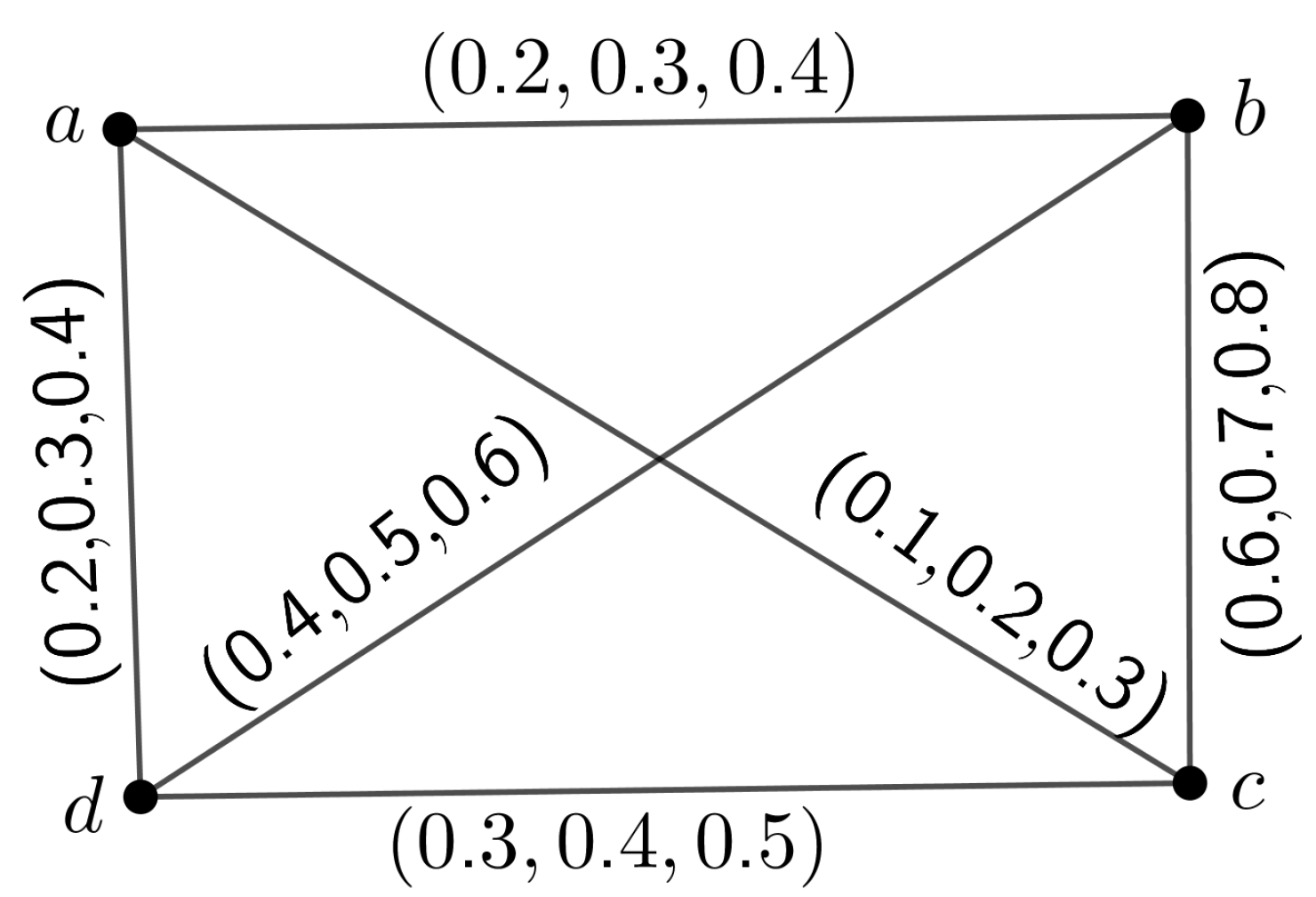
Example 1.

Here, we take a 3PFG, shown in Figure 1, to depict the above definitions. Here, we take into account all crisp nodes.

Here, the classified edges are given in

Table 2. Classification of edges of Figure 1.

Edge	Classification
$(a,b)$	$\beta$-strong
$(b,c)$	$\alpha$-strong
$(a,d)$	$\beta$-strong
$(b,d)$	$\alpha$-strong
$(a,c)$	$\delta$-strong
$(d,c)$	$\delta$-strong

.

α-node count of H is

$${\alpha }_V\left(H\right)=(\frac{0.6+0.4}{4},\frac{0.7+0.5}{4},\frac{0.8+0.6}{4})=(0.25,0.3,0.35)$$

and α-edge count of H is

$${\alpha }_E\left(H\right)=(\frac{0.6+0.4}{6},\frac{0.7+0.5}{6},\frac{0.8+0.6}{6})=(0.16,0.2,0.23)$$

β-node count of H is

$${\beta }_V\left(H\right)=(\frac{0.2+0.2}{4},\frac{0.3+0.3}{4},\frac{0.4+0.4}{4})=(0.1,0.15,0.2)$$

and β-edge count of H is

$${\beta }_E\left(H\right)=(\frac{0.2+0.2}{6},\frac{0.3+0.3}{6},\frac{0.4+0.4}{6})=(0.067,0.1,0.13)$$

Strong-node count of H is

$$S_V\left(H\right)=(\frac{1.4}{4},\frac{1.8}{4},\frac{2.2}{4})=(0.35,0.45,0.55)$$

and Strong-edge count of H is

$$S_E\left(H\right)=(\frac{1.4}{6},\frac{1.8}{6},\frac{2.2}{6})=(0.23,0.3,0.36)$$

Every edge in a mPF tree is $\alpha$-strong, according to Theorem 3.18 of [19]. Therefore, $p_s\circ {\alpha }_V\left(G\right)=\frac{n-1}{n}$ and $p_s\circ {\alpha }_E\left(G\right)=\frac{n-1}{n-1}=1$, where $n=$ no. of nodes in a mPF tree G as a whole.

The number of $\alpha$-strong nodes never surpasses the number of nodes for any other mPFG than the mPF tree. For a complete mPFG, all possible edges can be made $\beta$-strong by allotting the same MV to the nodes. Then $p_s\circ {\beta }_V\left(G\right)=\frac{\left(\genfrac{}{}{0pt}{}{n}{2}\right)}{2}$ and $p_s\circ {\beta }_E\left(G\right)=\frac{\left(\genfrac{}{}{0pt}{}{n}{2}\right)}{\left(\genfrac{}{}{0pt}{}{n}{2}\right)}=1$, $s=1\left(1\right)m$.

Depending on the above observation, we can say the following:

Proposition 1.

Suppose H is an mPFG where $\left|V\right|=n$. Then

(i) 

$0\le p_s\circ {\alpha }_V\left(H\right)\le \frac{n-1}{n}$.

(ii) 

$0\le p_s\circ {\alpha }_E\left(H\right)\le 1$.

(iii) 

$0\le p_s\circ {\beta }_V\left(H\right)\le \frac{\left(\genfrac{}{}{0pt}{}{n}{2}\right)}{2}$.

(iv) 

$0\le p_s\circ {\beta }_E\left(H\right)\le 1$.

(v) 

$0\le p_s\circ S_V\left(H\right)\le \frac{\left(\genfrac{}{}{0pt}{}{n}{2}\right)}{2}$.

(vi) 

$0\le p_s\circ S_E\left(H\right)\le 1$.

$s=1\left(1\right)m$.

Proposition 2.

Suppose H is an mPF tree. Then $0\le p_s\circ {\alpha }_V\left(H\right)\le p_s\circ {\alpha }_E\left(H\right)$, $s=1\left(1\right)m$.

Proof. 

As H is an mPF tree, therefore $p_s\circ {\alpha }_V\left(H\right)=\frac{n-1}{n}$, $s=1\left(1\right)m$ and $p_s\circ {\alpha }_E\left(H\right)=\frac{n-1}{n-1}=1$, $s=1\left(1\right)m$. Hence, $0\le p_s\circ {\alpha }_V\left(H\right)\le p_s\circ {\alpha }_E\left(H\right)$, $s=1\left(1\right)m$.    □

3.1. Vertex and Edge Counts of Some Well-Known mPFG

In this portion, we talk over saturation counts of mPFG structures such as mPF cycles, trees as well as blocks in mPFG. Some necessary parts for these structures are also obtained.

Theorem 1.

Suppose H is an mPFG where $\left|V\right|=w$. Then, the following condition is identical:

(i) 

H be an mPF tree.

(ii) 

$p_s\circ {\alpha }_V\left(H\right)=\frac{w-1}{w}$ as well as $p_s\circ {\alpha }_E\left(H\right)=1$, $s=1\left(1\right)m$.

(iii) 

$w\times p_s\circ {\alpha }_V\left(H\right)=(w-1)\times p_s\circ {\alpha }_E\left(H\right)$, $s=1\left(1\right)m$.

Proof. 

$\left(i\right)\Rightarrow \left(ii\right)$ is completed previously. $\left(ii\right)\Rightarrow \left(iii\right)$ Suppose that $p_s\circ {\alpha }_V\left(H\right)=\frac{w-1}{w}$ and $p_s\circ {\alpha }_E\left(H\right)=1$, $s=1\left(1\right)m$.

$$\begin{array}{cc}\hfill p_s\circ {\alpha }_V\left(H\right)& =\frac{w-1}{w}\hfill \\ \hfill \Rightarrow w\times p_s\circ {\alpha }_V\left(H\right)& =(w-1)\hfill \\ \hfill \Rightarrow w\times p_s\circ {\alpha }_V\left(H\right)& =(w-1)\times 1\hfill \\ \hfill \Rightarrow w\times p_s\circ {\alpha }_V\left(H\right)& =(w-1)\times p_s\circ {\alpha }_E\left(H\right)[As{p}_s\circ {\alpha }_E\left(H\right)=1]\hfill \end{array}$$

Hence, $n\times p_s\circ {\alpha }_V\left(H\right)=(w-1)\times p_s\circ {\alpha }_E\left(H\right)$, $s=1\left(1\right)m$. $\left(iii\right)\Rightarrow \left(i\right)$ Suppose that $w\times p_s\circ {\alpha }_V\left(H\right)=(w-1)\times p_s\circ {\alpha }_E\left(H\right)$, $s=1\left(1\right)m$.

Since,

$$\begin{array}{cc}\hfill w\times p_s\circ {\alpha }_V\left(H\right)& =(w-1)\times p_s\circ {\alpha }_E\left(H\right)\hfill \\ \hfill \Rightarrow \frac{p_s\circ {\alpha }_V\left(H\right)}{p_s\circ {\alpha }_E\left(H\right)}& =\frac{(w-1)}{w}\hfill \\ \hfill \Rightarrow \frac{p_s\circ {\alpha }_V\left(H\right)}{p_s\circ {\alpha }_E\left(H\right)}& =\frac{(w-1)}{w}=p_s\circ {\alpha }_V\left(H\right),\hfill \end{array}$$

this shows that $p_s\circ {\alpha }_E\left(H\right)=1$, $s=1\left(1\right)m$.

Hence, H is connected and acyclic only when every edge is $\alpha$-strong; therefore, H is a tree.   □

Theorem 2.

Suppose H is a connected mPFG. H is an mPF tree iff $p_s\circ {\alpha }_V\left(H\right)=p_s\circ S_V\left(H\right)$ as well as $p_s\circ {\alpha }_E\left(H\right)=p_s\circ S_E\left(H\right)$, $s=1\left(1\right)m$.

Proof. 

Suppose H is a connected mPFG as well as an mPF tree. Now, from Theorem 3.19 of [18], we know that H is free from $\beta$-SEs. Therefore,

$$p_s\circ {\beta }_V\left(H\right)=\frac{0}{\left|V\right|}=0,s=1\left(1\right)m$$

and

$$p_s\circ {\beta }_E\left(H\right)=\frac{0}{\left|E\right|}=0,s=1\left(1\right)m.$$

Therefore,

$$p_s\circ {\alpha }_V\left(H\right)=p_i\circ S_V\left(H\right),s=1\left(1\right)m$$

and

$$p_s\circ {\alpha }_E\left(H\right)=p_s\circ S_E\left(H\right),s=1\left(1\right)m.$$

Conversely, let $p_s\circ {\alpha }_V\left(H\right)=p_s\circ S_V\left(H\right)$ and $p_s\circ {\alpha }_E\left(H\right)=p_s\circ S_E\left(H\right)$, for $s=1,2,\dots ,m$. Whenever H defines a cycle, then H is an mPF tree. Take C to represent a cycle in H. Hence, C must have only $\alpha$-strong and $\delta$-SEs only. Again, consider that H does not have all $\alpha$-SEs. Therefore, H contains at least one $\delta$-SE. Suppose e is an $\delta$-SE. Then, we remove it from C. If a unique MST is found, then the condition is complete. Otherwise, we remove each $\delta$-SE individually from C until we get a specific MST of H.   □

Theorem 3.

Let a connected mPFG H be an mPF tree iff $p_s\circ {\alpha }_V\left(H\right)=p_s\circ {\alpha }_V\left(F\right)$, $s=1\left(1\right)m$, where F is MST of G.

Proof. 

Let H be an mPF tree. So, H and F are isomorphic. Therefore,

$$\begin{array}{cc}\hfill p_s\circ {\alpha }_V\left(H\right)& =\frac{countof\alpha -SEofH}{no.ofnodes}\hfill \\ \hfill & =\frac{countof\alpha -SEofF}{no.ofnodes}\hfill \\ \hfill & =p_s\circ {\alpha }_V\left(F\right)\hfill \end{array}$$

$s=1\left(1\right)m$.    □

Now, we consider another case. Let H contain a cycle C. Then, it is not free from $\delta$-SE. Let q be a $\delta$-SE. If $H-q$ is a tree, then $H-q$ and F are isomorphic. Therefore,

$$p_s\circ {\alpha }_V\left(H\right)=p_s\circ {\alpha }_V\left(F\right),s=1\left(1\right)m.$$

If $H-q$ is not a tree, then we delete the $\delta$-SEs in $H-e$ in a similar way to obtain an MST F of H, such that $p_s\circ {\alpha }_V\left(H\right)=p_s\circ {\alpha }_V\left(F\right)$, $s=1\left(1\right)m$.

Conversely, let $p_s\circ {\alpha }_V\left(H\right)=p_s\circ {\alpha }_V\left(F\right)$, $s=1\left(1\right)m$, in which F corresponds to H’s MST. We have to show that H is an mPF tree. Supposing H is not an mPF tree, it must have one $\beta$-SE, say $(a,b)$. Let $c-d$ be another path P in H for which $p_s\circ \mu (c,d)\ge p_s\circ \mu (a,b)$, $s=1\left(1\right)m$ and $\forall (c,d)\in P$. Now, the joining of P and $(a,b)$ creates a cycle in H. Let k be the count of $\alpha$-SEs, which are incident at a. To find F, take $(a,b)$ out of H since it has the least weight in C. Then the count of $\alpha$-SEs connected to c in F is $k+1$. Suppose the remaining counts of $\alpha$-SEs are $k_1$. Hence, $p_s\circ {\alpha }_V\left(H\right)=\frac{k+1}{\left|V\right|}$ as well as $p_s\circ {\alpha }_V\left(F\right)=\frac{k+k_1+1}{\left|V\right|}$, $s=1\left(1\right)m$, which is a contrast. This contradiction leads to the theorem.

4. Saturation in $\mathit{m}$-Polar Fuzzy Graph

Here, saturation in terms of the node and edge counts is presented. In this section, we also studied some of its interesting facts. We also studied saturated blocks in mPFG.

Definition 12.

Suppose H is an mPFG. Then H is called α-saturate ($\alpha -S$) if it must have one α-SEs incident with each node of H. H is said to be β-strong saturate if it must have one β-SE incident with each node of H.

Definition 13.

Suppose H is an mPFG. H is called a saturate graph if it has at least one α-SE as well as β-SEs incident with every node of H. Otherwise, H is called an unsaturated mPFG.

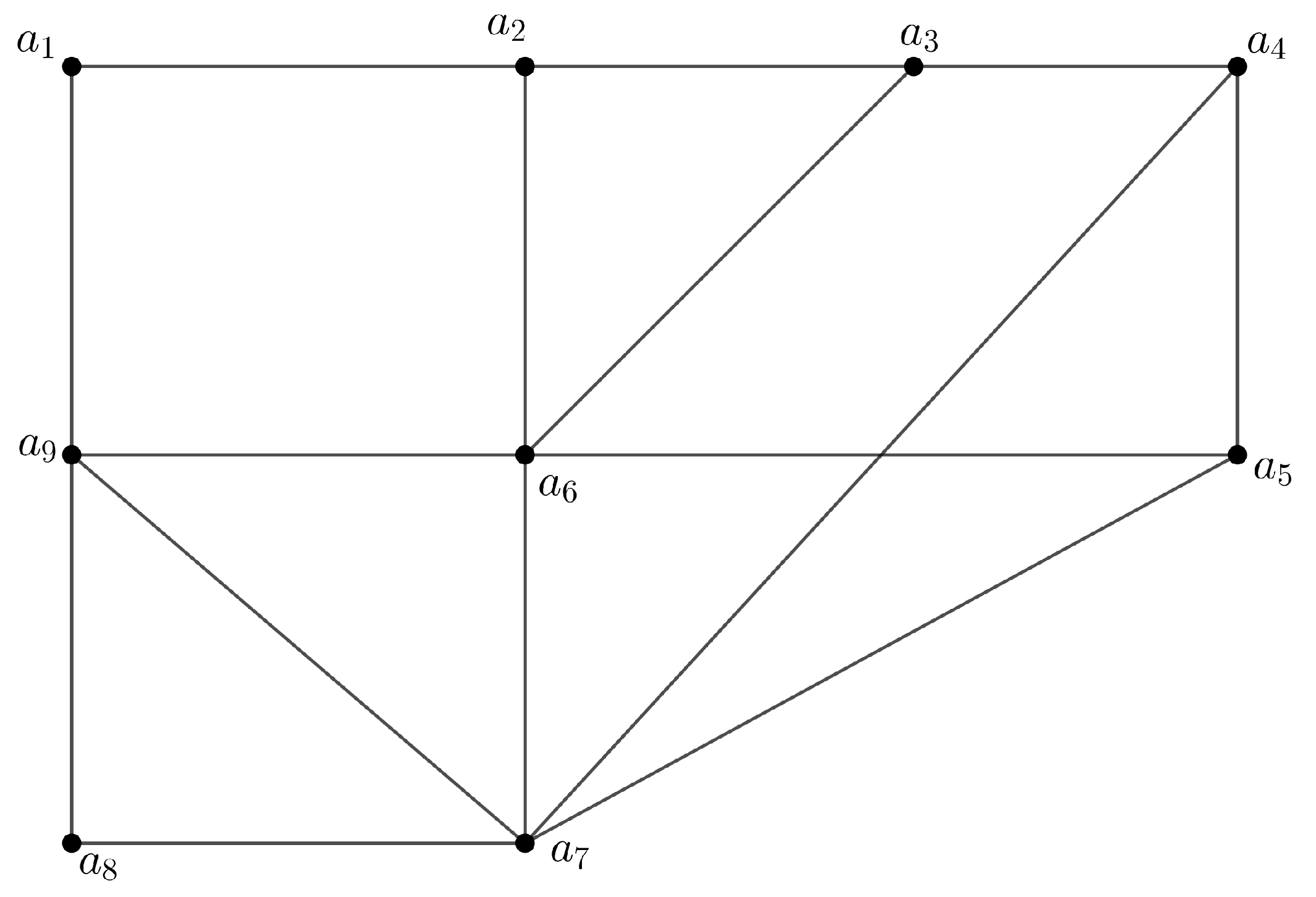
Example 2.

To illustrate the above definition, we consider a 3PFG H displayed in Figure 2 whose nodes all have MV $(1,1,1)$.

Here, we see that the edges $(a,b),(c,d)$ are α-SEs and $(c,b),(a,d)$ are β-SEs. The edges $(a,c)$ are δ-SE. Each node is connected with α-SE and β-SE. Therefore, H is a saturated 3PFG.

Theorem 4.

Suppose H as well as $H^{\prime }=(V^{\prime },{\sigma }^{\prime },{\mu }^{\prime })$ are two isomorphic mPFGs. If H is saturated, $H^{\prime }$ is also saturated.

Proof. 

Let $\varphi :H\to H^{\prime }$ be the isomorphism between two mPFGs. To show $H^{\prime }$ is saturated, we have to show that each node is connected with at least one $\alpha$-SE as well as $\beta$-SEs. Let $w^{\prime }\in V^{\prime }$. Then there must be a node, say w, in H for which $\varphi \left(w\right)=w^{\prime }$. Since H is saturated, therefore w is incident with at least one $\alpha$-SE and one $\beta$-SE. Since, H and $H^{\prime }$ are isomorphic with each other, therefore, $w^{\prime }$ is also incident with at least one $\alpha$-SE and one $\beta$-SE. Hence, $H^{\prime }$ is also saturated.

Let H be an mPFG having UCG $H^{\ast }$ where $\left|V\right|=k$. We define a finite collection ${\alpha }_S\left(H\right)=(n_1,n_2,\dots ,n_k)$ called $\alpha$-strong sequence where, $n_j=$ is the count of $\alpha$-SEs connected to node $v_j$. We define a finite collection ${\beta }_S\left(H\right)=(n_1,n_2,\dots ,n_k)$ called $\beta$-strong sequence where, $n_j=$ count of $\beta$-SEs connect at node $v_j$. Since the count of SEs of $H=$ (the count of $\alpha$-SEs of H + the count of $\beta$-SEs of H), therefore,

$$\sum _{n_j\in {\alpha }_S\left(H\right)}{n}_j+\sum _{n_j\in {\beta }_S\left(H\right)}{n}_j=\sum _{n_j\in S_S\left(H\right)}{n}_j$$

   □

Theorem 5.

Suppose H is an mPFG having UGC $H^{\ast }$ where $\left|V\right|=k$. Then H is α-saturated iff ${\displaystyle \sum _{n_j\in {\alpha }_S\left(H\right)}}{n}_j\ge k$.

Proof. 

Suppose H is an $\alpha$-saturated mPFG. Therefore, at least one $\alpha$-SE is incident with each node of H. Thus,

$$\begin{array}{cc}\hfill \sum _{n_j\in {\alpha }_S\left(H\right)}{n}_j& \ge 1+1+\dots +1\hfill \\ \hfill \Rightarrow \sum _{n_j\in {\alpha }_S\left(H\right)}{n}_j& \ge k\hfill \end{array}$$

Conversely, let ${\displaystyle \sum _{n_j\in {\alpha }_S\left(H\right)}}{n}_j\ge k$. Then, all k nodes of H are connected with at least one $\alpha$-SE. Therefore, H is $\alpha$-saturated mPFG.   □

Theorem 6.

Suppose H is an mPFG where $\left|V\right|=k$. Then H is β-saturated iff ${\displaystyle \sum _{n_j\in {\beta }_S\left(H\right)}}{n}_j\ge k$.

Proof. 

Similar to the above theorem.   □

Theorem 7.

Suppose H is an mPFG where $\left|V\right|=k$. If H is β-saturated, then ${\displaystyle \sum _{n_j\in S_S\left(H\right)}}{n}_j\ge 2k$.

Proof. 

Let H be saturated. Therefore, each node of H is connected with at least one $\alpha$-SE and one $\beta$-SE. Thus, ${\displaystyle \sum _{n_j\in S_S\left(H\right)}}{n}_j\ge 2k$.   □

Theorem 8.

Suppose H is an mPFG with UGC $H^{\ast }$ where $\left|V\right|=w$. If

(i) 

$p_s\circ {\alpha }_V\left(H\right)\ge 0.5$ if α-saturated.

(ii) 

$p_s\circ {\beta }_V\left(H\right)\ge 0.5$ if β-saturated.

(iii) 

$p_s\circ S_V\left(H\right)\ge 1$ if saturated.

$s=1\left(1\right)m$.

Proof. 

(i) Let H be $\alpha$-S. Then every node of H is incident with at least one $\alpha$-SE. Therefore, H must have $\frac{w}{2}$, $\alpha$-SEs. Therefore, $p_s\circ {\alpha }_V\left(H\right)\ge \frac{\frac{w}{2}}{w}=0.5$. (ii) Similar to the above. (iii) Let H be saturated. Therefore, every node of H is connected, having a minimum of $\alpha$-SEs and $\beta$-SEs. Therefore, the count of SEs of $H=$ (the count of $\alpha$-SEs of H + the count of $\beta$-SEs of H)$\ge \frac{w}{2}+\frac{w}{2}=n$. Hence, $p_s\circ S_V\left(H\right)\ge \frac{w}{w}=1$.   □

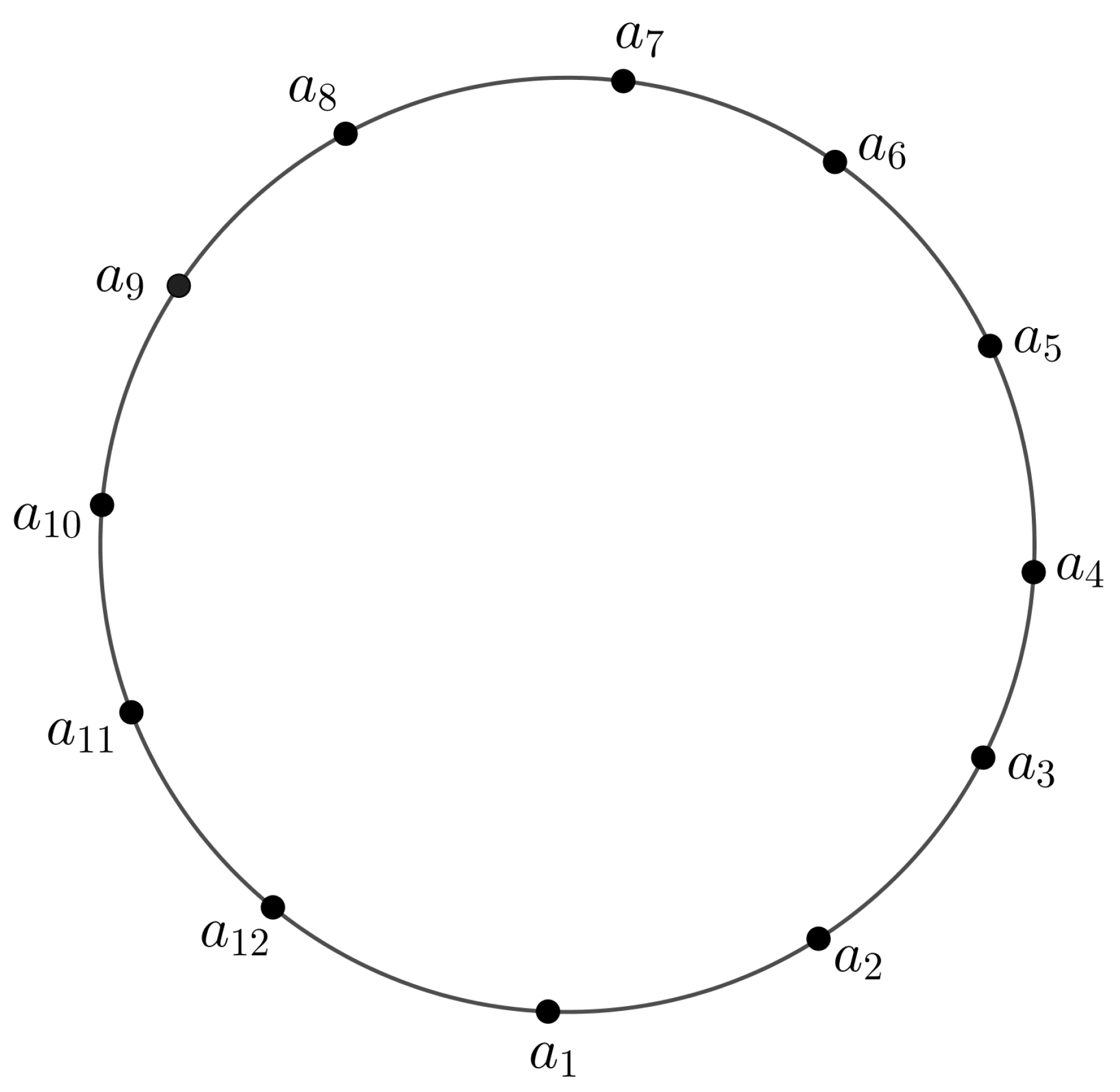
In Figure 3, all the nodes have MV $(1,1,1)$, that is $\sigma \left(a_j\right)=(1,1,1),forj=1,2,\dots ,12$. The edges MV are $\mu (a_j,a_k)=(0.6,0.6,0.6)$, where $1\le j<k\le 12$ and j is odd and k is even. The edges MV is $\mu (a_j,a_k)=(0.4,0.4,0.4)$, where $1<j<k<12$ and j is even and k is odd. The edge MV between $a_1$ and $a_{12}$ is $(0.4,0.4,0.4)$.

In Figure 3, we see that all the edges having MV $(0.6,0.6,0.6)$ are $\alpha$-strong and the edges having MV $(0.4,0.4,0.4)$ are $\beta$-strong. Therefore, Figure 3 is saturated.

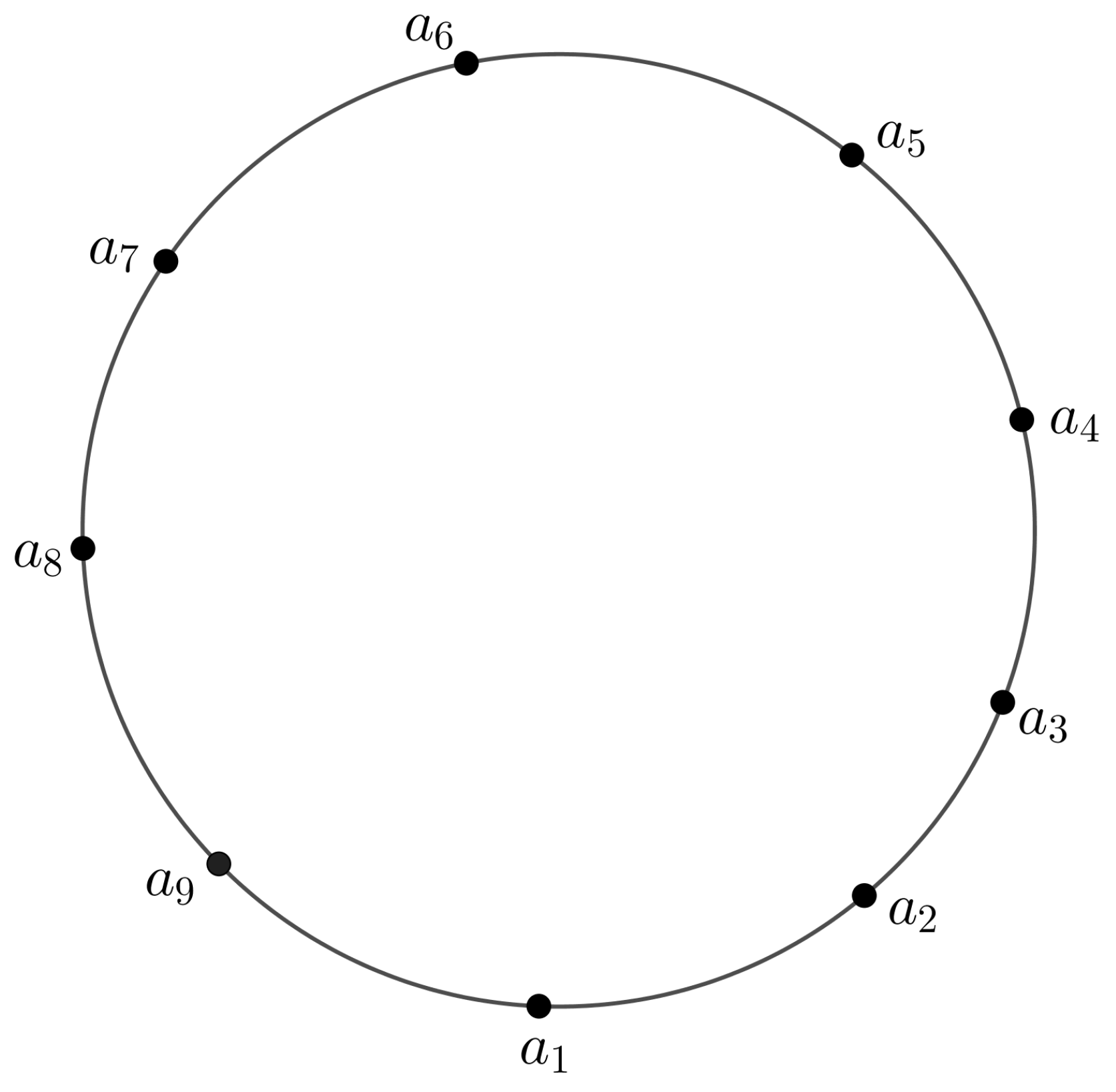
In Figure 4, all the nodes have MV $(1,1,1)$, that is $\sigma \left(a_j\right)=(1,1,1),forj=1,2,\dots ,9$. The edges MV is $\mu (a_j,a_k)=(0.5,0.5,0.5)$, where $1\le j<k\le 9$ and j is odd and k is even. The edges MV are $\mu (a_j,a_k)=(0.7,0.7,0.7)$, where $1<j<k<9$ and j is even and k is odd. The edge MV between $a_1$ and $a_9$ is $(0.5,0.5,0.5)$.

In Figure 4, we see that all the edges having MV $(0.7,0.7,0.7)$ are $\alpha$-strong and the edges having MV $(0.5,0.5,0.5)$ are $\beta$-strong. Therefore, Figure 4 is unsaturated as the node $a_1$ connected with both the $\beta$-SEs.

One simple observation of the above discussion is that Figure 3 has an even number of nodes while Figure 4 has an odd number of nodes. Thus, the next hypothesis applies.

Theorem 9.

Suppose $C_n$ is an mPF cycle. If the next two hold, it is saturated:

(i) 

$n=2t$, t is a positive integer.

(ii) 

α-SE as well as β-SEs occur as an alternate $C_n$.

Proof. 

Let $C_n$ be an mPF cycle. Therefore, it is free from $\delta$-SEs. All arcs occurring on $C_n$ are $\alpha$-SE or $\beta$-SE. Let us assume that $C_n$ is saturated. Therefore, each node is connected with at least one $\alpha$-SE and one $\beta$-SEs. Hence, the count of $\alpha$-SEs $=t$ = the count of $\beta$-SEs. Therefore, $n=2t$. Again, every node connected with both $\alpha$-SEs as well as $\beta$-SEs happen if they occur as an alternate $C_n$.   □

Conversely, let $C_n$ be a fuzzy cycle with an even number of nodes in which each node is connected with both $\alpha$-SEs and $\beta$-SEs alternatively. Therefore, each node is connected with precisely one $\alpha$-SE and $\beta$-SEs. Hence, $C_n$ is a saturated fuzzy cycle.

Theorem 10.

Suppose G is an mPF cycle. If H is saturated, it must be a block.

Proof. 

Since H is saturated, each node is connected with at least one $\alpha$-SE as well as one $\beta$-SE. Again, since H is an mPF cycle, every node is connected with just two nodes. Therefore, each node contains precisely one alpha-SE and one beta-SE. Hence, removing any node from H may not decrease SC between other nodes. This shows that H is free from mPF cut node; therefore, H is a block.   □

Theorem 11.

Let H be an mPF cycle. If H is an mPF block, then either it is β-saturated or it is saturated.

Proof. 

Let a block be H. We demand that H is free from $\delta$-SEs. If possible, let e be a $\delta$-SE. Then the remaining edges must be $\alpha$-SE; therefore, G contains $n-2$ fuzzy cut nodes, which is an irrelevance. So, H has no $\delta$-SEs. Thus, H is free from $\delta$-SEs.   □

If H has only $\alpha$-SEs as well as $\beta$-SEs, they appear alternatively; otherwise, the block shape will not be found. If the count of $\alpha$-SEs = the count of $\beta$-SEs =$\frac{n}{2}$, then H is $\alpha$-saturated as well as $\beta$-saturated; therefore, it is saturated. If the count of $\alpha$-SEs is less than the count of $\beta$-SEs, then H must be only $\beta$-S. For another case, when the count of $\alpha$-SEs is greater than the count of $\beta$-SEs, this will not be true as it does not form a block. If every of arc is $\beta$-strong of H, then it must be $\beta$-saturated. Therefore, the theorem is proved.

Theorem 12.

A complete mPFG has no δ-arcs.

Proof. 

Suppose G is a complete mPFG. Let G have a $\delta$-arc. Let $(p,q)$ be the $\delta$-arcs. Then we have,

$$p_s\circ \mu (p,q)<p_s\circ CON{N}_{G-(p,q)}\mu (p,q),s=1\left(1\right)m.$$

   □

In G, a stronger path P that excludes the arc $(p,q)$ must exist. Suppose $p_s\circ \mu (p,q)=t_i$, $s=1\left(1\right)m$ and the strength of P are $(u_1,u_2,\dots ,u_m)$. Therefore, we have $t_i<u_i$, $s=1\left(1\right)m$. Suppose r is the first node after u in the path P. Then, we have

$$p_s\circ \mu (p,r)>t_i,\forall s=1\left(1\right)m$$

(1)

In a similar way, let s be the last node before q in the path P. Again, we also have

$$p_s\circ \mu (s,q)>t_i,\forall s=1\left(1\right)m$$

(2)

Since G is a complete mPFG, we therefore have $p_s\circ \mu (p,t)=min\{p_s\circ \sigma \left(p\right),p_s\circ \sigma \left(t\right)\}$, $s=1\left(1\right)m$ as well as $\forall (p,t)\in E$. Therefore, at least one of $p_s\circ \sigma \left(p\right)$ or $p_s\circ \sigma \left(t\right)$ is $t_i$, $s=1\left(1\right)m$.

Therefore, $\left(1\right)$ will contradict if $p_s\circ \sigma \left(p\right)=t_i$, $s=1\left(1\right)m$ and $\left(2\right)$ will contradict if $p_s\circ \sigma \left(t\right)=t_i$, for $s=1\left(1\right)m$.

Hence, we conclude the theorem.

Theorem 13.

Suppose H is an mPFG. An arc $(a,c)$ is a bridge if it is α-strong.

Proof. 

Suppose $(a,c)$ is an mPF bridge. Then we have from the definition of mPF bridge,

$$p_s\circ CON{N}_{H-(a,c)}(a,c)<p_s\circ CON{N}_H(a,c), \mathrm{for} s=1\left(1\right)m$$

(3)

Again, from Theorem 3.11 of [19], we have

$$p_s\circ \mu (a,c)=p_s\circ CON{N}_H(a,c), s=1\left(1\right)m$$

(4)

From Equations $\left(3\right)$ and $\left(4\right)$, we get $p_s\circ \mu (a,c)>p_s\circ CON{N}_{H-(a,c)}(a,c)$, $s=1\left(1\right)m$. Hence, $(a,c)$ be $\alpha$-SE.

Conversely, suppose $(a,c)$ is an $\alpha$-SE. Then, we have $(a,c)$ as the one and only strongest path in between a and c, and the removal of $(a,c)$ will decrease the SC of a and c. Therefore, $(a,c)$ is a bridge.   □

Theorem 14.

A complete mPFG has at most one α-SE.

Proof. 

We know that complete mPFG have at most one mPF bridge. Again, from Theorem 13, we have an arc $(a,b)$ that is an mPF bridge iff it is $\alpha$-SE. Hence, a complete mPFG has at most one $\alpha$-SE.   □

Proposition 3.

Every complete mPFG has at most $\left(\genfrac{}{}{0pt}{}{w}{2}\right)$ or $\left(\genfrac{}{}{0pt}{}{w}{2}\right)$-1 β-SEs.

Theorem 15.

If H is a complete mPFG having w nodes, then few disparities hold.

(i) 

$0\le p_s\circ {\alpha }_V\left(H\right)\le \frac{1}{w}$.

(ii) 

$\frac{w^2-w-2}{2w}\le p_s\circ {\beta }_V\left(H\right)\le \frac{w-1}{2}$.

$s=1\left(1\right)m$.

Proof. 

With the help of Theorem 14, we conclude that H can have at most one $\alpha$-SE. Hence, we have $p_s\circ {\alpha }_V\left(H\right)\le \frac{1}{w}$, $s=1\left(1\right)m$. Again, clearly $p_s\circ {\alpha }_V\left(H\right)\ge 0$, $s=1\left(1\right)m$. Therefore, $0\le p_s\circ {\alpha }_V\left(H\right)\le \frac{1}{w}$, $s=1\left(1\right)m$.

Again, from Proposition 3, we are aware that the minimal number of $\beta$-SEs is $\left(\genfrac{}{}{0pt}{}{w}{2}\right)$−1. Therefore,

$$\begin{array}{cc}\hfill p_s\circ {\beta }_V\left(H\right)& \ge \frac{w\left(\frac{w-1}{2}\right)-1}{w}\hfill \\ \hfill & \ge \frac{w^2-w-2}{2w}\hfill \end{array}$$

Thus,$\frac{w^2-w-2}{2w}\le p_s\circ {\beta }_V\left(H\right)\le \frac{w-1}{2}$, $s=1\left(1\right)m$.

Next, we will try to find out the upper limit of the $\alpha$-node count for a block in mPFG.   □

Theorem 16.

If H is an mPF block, we have $p_s\circ {\alpha }_V\left(G\right)\le 0.5$, $s=1\left(1\right)m$.

Proof. 

To prove this, we first try to determine the maximum count of $\alpha$-SEs of H. Let $\left|V\right|=n$. We know that if more than one $\alpha$-SEs are connected with a common node, then the node is a mPF cut node. Since H is an mPF block, it therefore has no mPF cut node. Therefore, the maximum count of $\alpha$-SEs of H is $\frac{w}{2}$. Thus, $p_s\circ {\alpha }_V\left(H\right)\le \frac{\frac{w}{2}}{w}=0.5$, $s=1\left(1\right)m$.   □

Theorem 17.

An mPF block H is α-saturated then $p_s\circ {\alpha }_V\left(H\right)=0.5$, $s=1\left(1\right)m$.

Proof. 

Let H be $\alpha$-saturated. Since H is an mPF block, it therefore has no mPF cut node. Hence, every node is incident with exactly unique $\alpha$-SE. Therefore, H contains exactly $\frac{w}{2}$ the count of $\alpha$-SEs. Thus, $p_s\circ {\alpha }_V\left(H\right)=\frac{\frac{w}{2}}{w}=0.5$, for $s=1\left(1\right)m$.   □

5. Algorithms

In this section, three algorithms are designed to find $\alpha$-saturated mPFG, $\beta$-saturated mPFG and saturated mPFG.

Let $H^{\ast }=(V,E)$ be the crisp graph for the given mPFG.

Step 1 assigns the membership values to all nodes, and Step 2 does the same for all edges. So, the time complexities for these steps are $O\left(\right|V\left|\right)$ and $O\left(\right|E\left|\right)$, respectively. Finding connectedness between a pair of vertices is equivalent to finding all pairs’ shortest paths. Many algorithms are available to find all pairs of shortest paths, and their time complexity depends on the specific algorithm, data structure and type of graphs. Let such time complexity be $O\left(\chi \right(G\left)\right)$. So, the time complexity of Step 3 is $O\left(\chi \right(G\left)\right)$. Step 4 and Step 5 take $O\left(\right|E\left|\right)$ and $O\left(\right|V\left|\right)$, respectively. Step 6 takes only $O\left(\right|V\left|\right)$ time. Hence, the total time complexity of Algorithm 1 is $O\left(\right|V|+|E\left|\right)+O\left(\chi \right(G\left)\right)=O\left(\right|E|+\chi (G\left)\right)$. In the worst case, $O\left(\chi \left(G\right)\right)=O\left(\right|V{|}^3)$. So, the worst case time complexity of Algorithm 1 is $O\left(\right|V{|}^3)$, as the maximum value of $\left|E\right|$ is ${\left|V\right|}^2$.

The time complexities of Algorithms 2 and 3 are the same as in Algorithm  1.

Algorithm 1 An algorithm to find $\alpha$-saturation in mPFG

Input: A mPFG $H=(V,\sigma ,\mu )$. Output: Finding $\alpha$-saturated mPFG. Step 1: Put the MV of nodes $a_j$, $j=1\left(1\right)w$. Step 2: Put the MV of edges that satisfied $p_s\circ \mu (a_j,a_k)\le inf\{p_s\circ \sigma \left(a_j\right),p_s\circ \sigma \left(a_k\right)\}$, $s=1\left(1\right)m$. Step 3: Calculate $p_s\circ CON{N}_{H-\left((a_j,a_k)\right)}(a_j,a_k)$, $fors=1\left(1\right)m,\forall (a_j,a_k)\in E$. Step 4: Verify $p_s\circ \mu (a_j,a_k)>p_s\circ CON{N}_{H-(a_j,a_k)}(a_j,a_k)$, $\forall (a_j,a_k)\in E$. Step 5: Select all $\alpha$-SEs in H. Step 6: Check whether every node is connected with at least one $\alpha$-SE or not.

Algorithm 2 An algorithm to find $\beta$-saturation in mPFG

Input: A mPFG $H=(V,\sigma ,\mu )$. Output: Finding $\beta$-saturated mPFG. Step 1: Put the MV of nodes $a_j$, $j=1\left(1\right)w$. Step 2: Put the MV of edges that satisfied $p_s\circ \mu (a_j,a_k)\le inf\{p_s\circ \sigma \left(a_j\right),p_s\circ \sigma \left(a_k\right)\}$, $s=1\left(1\right)m$. Step 3: Find $p_s\circ CON{N}_{H-\left((a_j,a_k)\right)}(a_j,a_k)$, $fors=1\left(1\right)m,\forall (a_j,a_k)\in E$. Step 4: Verify $p_s\circ \mu (a_j,a_k)=p_s\circ CON{N}_{H-(a_j,a_k)}(a_j,a_k)$, $\forall (a_j,a_k)\in E$. Step 5: Select all $\beta$-SEs in H. Step 6: Check whether every node is connected with at least one $\beta$-SE or not.

Algorithm 3 An algorithm to find saturation in mPFG

Input: A mPFG $H=(V,\sigma ,\mu )$. Output: Finding saturated mPFG. Step 1: Put the MV of nodes $a_j$, $j=1\left(1\right)w$. Step 2: Put the MV of edges that satisfied $p_s\circ \mu (a_j,a_k)\le inf\{p_s\circ \sigma \left(a_j\right),p_s\circ \sigma \left(a_k\right)\}$, $s=1\left(1\right)m$. Step 3: Using Algorithms 1 and 2 identified all $\alpha$-strong as well as $\beta$-SEs in G. Step 4: Check whether every node is connected with at least one $\alpha$-SE as well as $\beta$-SEs or not.

6. Application

Decision-making in allocation problems is a multifaceted process that requires a systematic approach, consideration of various factors, and a balance between optimizing objectives and meeting constraints. Effective decision-making in allocation can lead to improved resource utilization, cost savings, and overall better outcomes for organizations and society. The mPFG is a fundamental mathematical framework that depicts facts from real life that are related by graphical systems, where nodes and edges are made up of m-polar fuzzy information. In this section, we attempt to resolve a specific allocation problem using saturation in mPFG.

6.1. Model Construction

Education is a crucial concern for everyone in the current world. Everyone gets the chance to read and write thanks to the 2005 Right to Education (RTE) law. IIT (Indian Institute of Technology) is one of the most significant universities in India’s educational system. Therefore, it is not a simple undertaking for any Government to construct an IIT in a town among other towns.

In this case, nine towns ($a_1,a_2,\dots ,a_9$) are regarded as nodes. If there is a road link between two nodes, then there will be an edge. Here, we use saturation in 3PFG G to solve the allocation problem. Since the town is fixed in nature, we can therefore assign the MV of each node $(1,1,1)$, that is, $\sigma \left(a_i\right)=(1,1,1)$, for $i=1,2,\dots ,9$. The edge MVs are calculated depending on three criteria. Those criteria are as follows: {Condition of roads, traffic jams on the roads, communication system between two cities}. All the indicators of an edge between two towns are uncertain in nature. We can calculate the edge MVs by remembering the relation $p_s\circ \mu (a,c)\le inf\{p_s\circ \sigma \left(a\right),p_s\circ \sigma \left(c\right)\}$, $s=1\left(1\right)m$. The model 3PFG is shown in Figure 5.

Here, the edges MV are given in

Table 3. The edge membership value of Figure 5.

Edge	Membership Value
$(a_1,a_2)$	$(0.5,0.4,0.3)$
$(a_2,a_3)$	$(0.5,0.4,0.3)$
$(a_3,a_4)$	$(0.3,0.2,0.1)$
$(a_4,a_5)$	$(0.3,0.2,0.1)$
$(a_5,a_7)$	$(0.6,0.5,0.4)$
$(a_7,a_8)$	$(0.5,0.4,0.3)$
$(a_8,a_9)$	$(0.3,0.2,0.1)$
$(a_1,a_9)$	$(0.7,0.6,0.5)$
$(a_7,a_9)$	$(0.6,0.5,0.4)$
$(a_6,a_9)$	$(1,0.9,0.8)$
$(a_6,a_7)$	$(0.6,0.5,0.4)$
$(a_5,a_6)$	$(0.6,0.5,0.4)$
$(a_2,a_6)$	$(0.8,0.7,0.6)$
$(a_3,a_6)$	$(0.5,0.4,0.3)$
$(a_4,a_7)$	$(0.7,0.6,0.5)$

.

6.2. Illustration of Membership Values

Here, the model network system contains nine nodes and fifteen edges. It can be seen from the given 3PFG that every town is connected to others through some paths. So, first, we want to check whether the connections between towns are $\alpha$, $\beta$ or $\delta$-strong. Next, we find out the saturation node in Figure 5. After calculating $CON{N}_{G-(a,b)}$, for all $(a,b)\in E$, we find out which edges are $\alpha$, $\beta$ or $\delta$-strong. Then, by the routine computations, we get the classification of edges. Here, the classified edges are given in

Table 4. Classification of edges of Figure 5.

Edge	Classification
$(a_1,a_2)$	$\delta$-strong
$(a_2,a_3)$	$\delta$-strong
$(a_3,a_4)$	$\delta$-strong
$(a_4,a_5)$	$\delta$-strong
$(a_5,a_7)$	$\delta$-strong
$(a_7,a_8)$	$\alpha$-strong
$(a_8,a_9)$	$\delta$-strong
$(a_1,a_9)$	$\alpha$-strong
$(a_7,a_9)$	$\delta$-strong
$(a_6,a_9)$	$\alpha$-strong
$(a_6,a_7)$	$\delta$-strong
$(a_5,a_6)$	$\delta$-strong
$(a_2,a_6)$	$\alpha$-strong
$(a_3,a_6)$	$\beta$-strong
$(a_4,a_7)$	$\alpha$-strong

.

We can observe that the model 3PFG G only has one $\beta$-SE. The node $a_6$, which is incident with at least one $\alpha$-SE and one $\beta$-SE, is the sole saturation node in the model 3PFG G.

6.3. Decision Making

The town $a_6$ is the most favourable location to set up the IIT (Indian Institute of Technology) among all the towns taken into consideration in our suggested model since it is the sole saturation node in the model 3PFG G. Decision-making in allocation problems is critical to operations management and resource allocation across various domains, including business, logistics, healthcare, and government. Allocation problems involve distributing limited resources among competing demands or tasks in an optimal or efficient manner. These decisions play a significant role in determining the overall performance, cost-effectiveness, and fairness of an allocation process.

We know that saturation in mPFG plays an important role in this allocation problem through the above discussion. Moreover, we also recognize that saturation in mPFG is more applicable than saturation in FG in the allocation problem.

Comparative study

First, Mathew et al. [10] introduced a saturation graph in the light of fuzziness. Later on, Mathew et al. [6,7] also worked on different properties of saturated FGs. So, none of the results discussed earlier are applicable when the model is considered in another environment, such as in m-polar fuzzy sets. This is why the proposed model in this paper plays a significant role in such situations to give better results.

Advantages and limitations of the proposed Work

Some of the advantages of the proposed work are as follows:

(i)

This work mainly depends on m-polar fuzzy logic network system.

(ii)

Many important definitions and theorems are presented in this study, which are very useful.

(iii)

A real application of a m-polar fuzzy saturation graph is presented in the allocation problem system.

Some of the limitations of this study are given as follows:

(i)

This work mainly focuses on the m-polar fuzzy graph.

(ii)

If the membership value of the character is given in a different interval-valued m-polar fuzzy environment, then the m-polar fuzzy threshold graph cannot be used.

(iii)

This type of work is mainly used in allocation problems.

7. Conclusions

In this paper, $\alpha$-saturation and $\beta$-saturation in mPFG, along with its several properties, are initiated. Node, as well as edge saturation count in mPFG and a few of its facts on some well-known mPFGs, are also introduced. The upper and lower bound of a node and edge saturation count in mPFG are also investigated. Saturation in mPFG by using $\alpha$-saturation and $\beta$-saturation are also discussed here, along with some of its intersecting properties. Using saturation in mPFG, an application is also given in the last part of this paper. Depending on the mPFG, our research will be expanded to uncover other traits and potential uses. To the best of our knowledge, no work has been conducted on $\alpha$-saturation and $\beta$-saturation before this present work on mPFG. Several results have been presented in this paper. The connection between $\alpha$-saturation and $\beta$-saturation is not established here. This should be conducted in later work. Until now, the saturation on interval-valued m-polar fuzzy soft graphs, saturation on balanced IVmPF graphs, and saturation on self-centered IVmPF graphs were not investigated by any researchers.