Article

Some Results in Fuzzy b-Metric Space with b-Triangular Property and Applications to Fredholm Integral Equations and Dynamic Programming

1
Department of Mathematics, Saveetha School of Engineering, Saveetha Institute of Medical and Technical Sciences, Chennai 602105, Tamil Nadu, India
2
Department of Mathematics, Faculty of Engineering and Technology, SRM Institute of Science and Technology, SRM Nagar, Kattankulathur 603203, Tamil Nadu, India
3
Department of Pharmaceutical Sciences, “Vasile Goldiş” Western University of Arad, L. Rebreanu Street, No. 86, 310048 Arad, Romania
4
Department of Mathematics, College of Science and Humanities in Alkharj, Prince Sattam bin Abdulaziz University, Al-Kharj 11942, Saudi Arabia
5
Faculty of Electrical Engineering, University of Banja Luka, Patre 5, 78000 Banja Luka, Bosnia and Herzegovina
*
Author to whom correspondence should be addressed.
Mathematics 2023, 11(19), 4101; https://doi.org/10.3390/math11194101
Submission received: 13 May 2023 / Revised: 19 June 2023 / Accepted: 20 June 2023 / Published: 28 September 2023

Abstract

:
In this paper, we introduce the b-triangular property in fuzzy b-metric space. Furthermore, we give some new fixed point results in fuzzy b-metric space for non-continuous mappings. Our results generalize and expand some results from the related literature. Two applications of our results, to solving Fredholm integral equation and in dynamic programming, are also given.

1. Introduction and Preliminaries

The concept of continuous triangular norm was given by Schweizer and Sklar [1] in 1960. In 1965, the theory of fuzzy sets was given by Zadeh [2]. Later, in 1975, Kramosil and Michalek (see [3]), starting with the notion of fuzzy sets, defined the concept of fuzzy metric space with the continuous t-norms. The premise that there does not necessarily have to be a real number to describe the distance between two points is the basis for the fuzzy approach to distance. Then, in the same frame, George and Veeramani [4], in 1994, changed the definition of the fuzzy metric spaces. In [5], Grabeic gave the well-known Banach contraction principle in the case of fuzzy metric spaces, in the sense of Kramosil and Michalek. Starting with this generalization, many other researchers extended these results. One important case is that of Gregori and Sapena (see [6]), where the fuzzy Banach contraction theorem is translated in the case of fuzzy metric space in the sense of George and Veeramani [4]. Recently, were developed the fixed point theory fuzzy b-metric spaces. For example, see the generalizations of Sedghi and Shobe [7] and Abbas et al. [8]. The notion of the triangular property of the fuzzy metric in fuzzy metric spaces was given by Shamas et al. [9] in order to prove fixed point results losing the continuity condition. Moreover, many results on fuzzy metric spaces can be consulted in the following research works [10,11,12,13,14,15,16,17,18,19,20,21,22,23,24,25,26,27,28].
Furthermore, we give some basic definitions below:
Definition 1
([7]). A 3-tuple ( U , M r , ) is said to be a fuzzy b-metric space (FBM space) if U is an arbitrary (non-empty) set, ∗ is a continuous ϑ-norm and M r is a fuzzy set on U 2 × ( 0 , + ) , satisfying the following conditions:
(F1)
M r ( υ , ϖ , ϑ ) > 0 ,
(F2)
M r ( υ , ϖ , ϑ ) = 1 if and only if υ = ϖ ,
(F3)
M r ( υ , ϖ , ϑ ) = M r ( ϖ , υ , ϑ ) ,
(F4)
M r ( υ , ϖ , s ( ϑ + g ) ) M r ( υ , ξ , ϑ ) M r ( ξ , ϖ , g ) ,
(F5)
M r ( υ , ϖ , . ) : ( 0 , + ) [ 0 , 1 ] is continuous,
for all υ , ϖ , ξ U , ϑ , g > 0 and s 1 . The function M r is said to be a fuzzy b-metric.
Definition 2
([8]). Let ( U , M r , ) be a FBM space.
(D1)
A sequence { υ κ } is convergent and converges to υ U if lim κ + M r ( υ κ , υ , ϑ ) = 1 for all ϑ > 0 and denoted υ κ υ as κ + .
(D2)
If lim κ , k + M r ( υ κ , υ k , ϑ ) = 1 and for any ϑ > 0 then { υ κ } is said to be a Cauchy sequence in U .
(D3)
If every Cauchy sequence is convergent in U then U is said to be a complete FBM space.
Definition 3.
Let ( U , M r , ) be an FBM-space with s 1 and a mapping 𝓁 : U U is called fuzzy b-contraction if there exists δ 1 ( 0 , 1 ) such that
1 M r ( 𝓁 υ 1 , 𝓁 υ * , ϑ ) 1 δ 1 1 M r ( υ 1 , υ * , ϑ ) 1 ,
for all υ 1 , υ * , U , ϑ > 0 .
Definition 4.
Let ( U , M r , ) be an FBM-space with s 1 and a mapping 𝓁 : U U is said to be a rational type fuzzy b-contraction if there exists δ 1 ( 0 , 1 ) and δ 2 0 s.t:
1 M r ( 𝓁 υ 1 , 𝓁 υ * , ϑ ) 1 δ 1 1 M r ( υ 1 , υ * , ϑ ) 1 + δ 2 M r ( υ 1 , υ * , ϑ ) M r ( υ 1 , 𝓁 υ 1 , ϑ ) * M r ( υ * , 𝓁 υ 1 , 2 s ϑ ) 1 ,
for all υ 1 , υ * , U , ϑ > 0 .
In this manuscript, we prove some results of fixed points in the fuzzy b-metric spaces for non-continuous mappings. Motivated by the solutions of Shamas et al. [9] and Mani et al. [29] we recall the b-triangular property in fuzzy b-metric space, which is crucial for proving the new results here presented. Furthermore, we give some interesting applications of our results, the first result for proving the existence of a unique result of an integral Fredholm equation, and the other in dynamic programming.

2. Main Results

In this section, we recall first the b-triangular property given by Mani et al. in [29] and we discuss some new fixed point results involving this condition. We can say that it is an interesting way to prove the existence of a fixed point considering the b-triangular property, without having the property of continuity of the fuzzy b-metric. Then we give a result of fixed points for rational-type fuzzy b-contractions that satisfy condition (2).
First, let us recall the b-triangular property of a fuzzy b-metric in an F B M space.
Definition 5
([29]). Let ( U , M r , ) be an FBM space with s 1 . The fuzzy b-metric M r is b-triangular if:
1 M r ( υ , ϖ , ϑ ) 1 s 1 M r ( υ , ξ , ϑ ) 1 + 1 M r ( ξ , ϖ , ϑ ) 1
Remark 1.
Note that, if s = 1 , we obtain the triangular property defined by Bari and Vetro [30].
Example 1
([29]). Let M r : U 2 × ( 0 , + ) [ 0 , 1 ] be defined by:
M r ( υ , ϖ , ϑ ) = ϑ ϑ + | υ ϖ | 2 ,
for all υ , ϖ U , ϑ > 0 .
Now,
1 M r ( υ , ϖ , ϑ ) 1 = | υ ϖ | 2 ϑ = | υ ξ + ξ ϖ | 2 ϑ 2 | υ ξ | 2 ϑ + | ξ ϖ | 2 ϑ = 2 1 M r ( υ , ξ , ϑ ) 1 + 1 M r ( ξ , ϖ , ϑ ) 1
which implies that:
1 M r ( υ , ϖ , ϑ ) 1 s 1 M r ( υ , ξ , ϑ ) 1 + 1 M r ( ξ , ϖ , ϑ ) 1 ,
for ϑ > 0 , where s = 2 . So, M r is fuzzy b-triangular.
Our first main result is the following.
Theorem 1
(Banach contraction principle in FBM). Let ( U , M r , ) be a complete FBM-space with s 1 s.t M r is b-triangular and a mapping 𝓁 : U U is a fuzzy b-contraction satisfying (1). Then, ℓ has a UFP (unique fixed point) in U .
Proof. 
Fix υ 0 U and υ κ + 1 = 𝓁 υ κ , κ 0 . Then, by (1), for ϑ > 0 , κ 1 , we have:
1 M r ( υ κ , υ κ + 1 , ϑ ) 1 = 1 M r ( 𝓁 υ κ 1 , 𝓁 υ κ , ϑ ) 1 δ 1 1 M r ( υ κ 1 , υ κ , ϑ ) 1 .
Then,
1 M r ( υ κ , υ κ + 1 , ϑ ) 1 δ 1 1 M r ( υ κ 1 , υ κ , ϑ ) 1 .
Now, from (3) using induction, we have:
1 M r ( υ κ , υ κ + 1 , ϑ ) 1 δ 1 κ 1 M r ( υ 0 , υ 1 , ϑ ) 1
for ϑ > 0 . So,
lim κ + M ( υ κ , υ κ 1 , ϑ ) = 1 ,
for ϑ > 0 . Since M r is b-triangular, using (4) we obtain:
1 M r ( υ κ , υ k , ϑ ) 1 s 1 M r ( υ κ , υ κ + 1 , ϑ ) 1 + 1 M r ( υ κ + 1 , υ k , ϑ ) 1 s 1 M r ( υ κ , υ κ + 1 , ϑ ) 1 + s 2 1 M r ( υ κ + 1 , υ κ + 2 , ϑ ) 1
+ + s k κ 1 1 M r ( υ k 1 , υ k , ϑ ) 1 ( s δ 1 κ + s 2 δ 1 κ + 1 + + s k κ 1 δ 1 k 1 ) 1 M r ( υ 0 , υ 1 , ϑ ) 1 s δ 1 κ 1 s δ 1 1 M r ( υ 0 , υ 1 , ϑ ) 1 0 , as   κ + .
Therefore, { υ κ } is a Cauchy sequence in U . Since ( U , M r , ) is complete, there is ϖ 1 U such that
lim κ + M r ( υ κ , ϖ 1 , ϑ ) = 1 ,
for ϑ > 0 . Since M r is a b-triangular, from (1), (5) and (6), for ϑ > 0 , we have:
1 M r ( ϖ 1 , 𝓁 ϖ 1 , ϑ ) 1 s 1 M r ( ϖ 1 , υ κ + 1 , ϑ ) 1 + s 1 M r ( 𝓁 υ κ , 𝓁 ϖ 1 , ϑ ) 1 s 1 M r ( ϖ 1 , υ κ + 1 , ϑ ) 1 + s δ 1 1 M r ( υ κ , ϖ 1 , ϑ ) 1 = s 1 M r ( ϖ 1 , υ κ + 1 , ϑ ) 1 + s δ 1 1 M r ( υ κ , ϖ 1 , ϑ ) 1 0   as   κ + .
Hence,
M r ( ϖ 1 , 𝓁 ϖ 1 , ϑ ) = 1 .
Therefore,
𝓁 ϖ 1 = ϖ 1 ,
for ϑ > 0 . Let z 1 U s.t 𝓁 z 1 = z 1 and 𝓁 z 1 ϖ 1 ; then, from (1) we obtain:
1 M r ( ϖ 1 , z 1 , ϑ ) 1 = 1 M r ( 𝓁 ϖ 1 , 𝓁 z 1 , ϑ ) 1 δ 1 1 M r ( ϖ 1 , z 1 , ϑ ) 1 < 1 M r ( ϖ 1 , z 1 , ϑ ) 1 .
This is a contradiction. So, ϖ 1 = z 1 . □
Example 2.
Consider U = [ 0 , + ) , ∗ to be a continuous ϑ-norm and M r : U 2 × ( 0 , + ) [ 0 , 1 ] by:
M r ( υ , ϖ , ϑ ) = ϑ ϑ + | υ 1 υ * | 2 ,
for all υ 1 , υ * U , ϑ > 0 . Clearly, M r is b-triangular and ( M r , ) is a complete FBM space with s = 2 (see Example 1). Define 𝓁 : U U by:
𝓁 ( υ 1 ) = υ 1 3 ,
for all υ 1 U . Then we have:
1 M r ( 𝓁 ( υ 1 ) , 𝓁 ( υ * ) , ϑ ) 1 = 1 3 1 M r ( υ 1 , υ * , ϑ ) 1
Thereby, all the axioms of Theorem 1 are fulfilled with δ 1 = 1 3 ( 0 , 1 2 ) . Hence ℓ has a UFP υ 1 = 0 .
Our next main theorem is given below:
Theorem 2.
Let ( U , M r , ) be a complete FBM-space with s 1 s.t M r is b-triangular and a mapping 𝓁 : U U is a rational-type fuzzy b-contraction satisfying (2) s.t δ 1 ( 0 , 1 s ) and δ 2 0 . Then, ℓ has a UFP in U .
Proof. 
Fix υ 0 U and υ κ + 1 = 𝓁 υ κ , κ 0 . Then, by (2), for ϑ > 0 , κ 1 , we have:
1 M r ( υ κ , υ κ + 1 , ϑ ) 1 = 1 M r ( 𝓁 υ κ 1 , 𝓁 υ κ , ϑ ) 1 δ 1 1 M r ( υ κ 1 , υ κ , ϑ ) 1 + δ 2 M r ( υ κ 1 , υ κ , ϑ ) M r ( υ κ 1 , 𝓁 υ κ 1 , ϑ ) M r ( υ κ , 𝓁 υ κ 1 , 2 s ϑ ) 1 = δ 1 1 M r ( υ κ 1 , υ κ , ϑ ) 1 + δ 2 M r ( υ κ 1 , υ κ , ϑ ) M r ( υ κ 1 , υ κ , ϑ ) M r ( υ κ , υ κ , 2 s ϑ ) 1 .
Then,
1 M r ( υ κ , υ κ + 1 , ϑ ) 1 δ 1 1 M r ( υ κ 1 , υ κ , ϑ ) 1 .
Now, from (7) using induction, we have:
1 M r ( υ κ , υ κ + 1 , ϑ ) 1 δ 1 κ 1 M r ( υ 0 , υ 1 , ϑ ) 1
for ϑ > 0 . So,
lim κ + M ( υ κ , υ κ 1 , ϑ ) = 1 ,
for ϑ > 0 . Since M r is b-triangular, using (8) we obtain:
1 M r ( υ κ , υ k , ϑ ) 1 s 1 M r ( υ κ , υ κ + 1 , ϑ ) 1 + 1 M r ( υ κ + 1 , υ k , ϑ ) 1 s 1 M r ( υ κ , υ κ + 1 , ϑ ) 1 + s 2 1 M r ( υ κ + 1 , υ κ + 2 , ϑ ) 1 + + s k κ 1 1 M r ( υ k 1 , υ k , ϑ ) 1 ( s δ 1 κ + s 2 δ 1 κ + 1 + + s k κ 1 δ 1 k 1 ) 1 M r ( υ 0 , υ 1 , ϑ ) 1 s δ 1 κ 1 s δ 1 1 M r ( υ 0 , υ 1 , ϑ ) 1 0 , as   κ + .
Therefore, { υ κ } is a Cauchy sequence in U . Since ( U , M r , ) is complete, there is ϖ 1 U such that:
lim κ + M r ( υ κ , ϖ 1 , ϑ ) = 1 ,
for ϑ > 0 . Since M r is a b-triangular, from (2), (9) and (10), for ϑ > 0 , we have:
1 M r ( ϖ 1 , 𝓁 ϖ 1 , ϑ ) 1 s 1 M r ( ϖ 1 , υ κ + 1 , ϑ ) 1 + s 1 M r ( 𝓁 υ κ , 𝓁 ϖ 1 , ϑ ) 1 s 1 M r ( ϖ 1 , υ κ + 1 , ϑ ) 1 + s δ 1 1 M r ( υ κ , ϖ 1 , ϑ ) 1 + s δ 2 M r ( υ κ , ϖ 1 , ϑ ) M r ( υ κ , 𝓁 υ κ , ϑ ) M r ( ϖ 1 , 𝓁 υ κ , 2 s ϑ ) 1 = s 1 M r ( ϖ 1 , υ κ + 1 , ϑ ) 1 + s δ 1 1 M r ( υ κ , ϖ 1 , ϑ ) 1 + s δ 2 M r ( υ κ , ϖ 1 , ϑ ) M r ( υ κ , υ κ + 1 , ϑ ) M r ( ϖ 1 , υ κ + 1 , 2 s ϑ ) 1 0   as   κ + .
Hence,
M r ( ϖ 1 , 𝓁 ϖ 1 , ϑ ) = 1 .
Therefore,
𝓁 ϖ 1 = ϖ 1 ,
for ϑ > 0 . Let z 1 U s.t 𝓁 z 1 = z 1 and 𝓁 z 1 ϖ 1 ; then, from (2) we obtain:
1 M r ( ϖ 1 , z 1 , ϑ ) 1 = 1 M r ( 𝓁 ϖ 1 , 𝓁 z 1 , ϑ ) 1 δ 1 1 M r ( ϖ 1 , z 1 , ϑ ) 1 + δ 2 M r ( ϖ 1 , z 1 , ϑ ) M r ( ϖ 1 , 𝓁 ϖ 1 , ϑ ) M r ( z 1 , 𝓁 ϖ 1 , 2 s ϑ ) 1 δ 1 1 M r ( ϖ 1 , z 1 , ϑ ) 1 + δ 2 M r ( ϖ 1 , z 1 , ϑ ) M r ( z 1 , ϖ 1 , ϑ ) M r ( ϖ 1 , ϖ 1 , ϑ ) 1 = δ 1 1 M r ( ϖ 1 , z 1 , ϑ ) 1 < 1 M r ( ϖ 1 , z 1 , ϑ ) 1 .
This is a contradiction. So, ϖ 1 = z 1 . □
Next, let us give another fixed point result related to b-triangular property of the fuzzy metric.
Theorem 3.
Let ( U , M r , ) be a complete FBM-space with s 1 , s.t M r is b-triangular and a mapping 𝓁 : U U that satisfies:
1 M r ( 𝓁 υ 1 , 𝓁 υ * , ϑ ) 1 δ 1 1 M r ( υ 1 , υ * , ϑ ) 1 + δ 2 M r ( υ 1 , υ * , ϑ ) M r ( υ 1 , 𝓁 υ * , ϑ ) M r ( υ 1 , 𝓁 υ 1 , ϑ ) M r ( υ 1 , 𝓁 υ * , 2 s ϑ ) 1 + δ 3 M r ( υ 1 , 𝓁 υ 1 , ϑ ) M r ( υ 1 , 𝓁 υ * , 2 s ϑ ) 1 + M r ( υ * , 𝓁 υ * , ϑ ) M r ( 𝓁 υ 1 , 𝓁 υ * , 2 s ϑ ) 1 + δ 4 1 M r ( υ 1 , 𝓁 υ 1 , ϑ ) 1 + 1 M r ( υ * , 𝓁 υ * , ϑ ) 1 ,
for all υ 1 , υ * M , ϑ > 0 , δ i 0 , i = 1 , 2 , 3 , 4 with δ 1 + δ 2 + 2 δ 3 + 2 δ 4 < 1 s . Then ℓ has a UFP.
Proof. 
Fix υ 0 U and υ κ + 1 = 𝓁 υ κ , κ 0 . Then, by (11), for ϑ > 0 , κ 1 , we have:
1 M r ( υ κ , υ κ + 1 , ϑ ) 1 = 1 M r ( 𝓁 υ κ 1 , 𝓁 υ κ , ϑ ) 1 δ 1 1 M r ( υ κ 1 , υ κ , ϑ ) 1 + δ 2 M r ( υ κ 1 , υ κ , ϑ ) M r ( υ κ , 𝓁 υ κ , ϑ ) M r ( υ κ 1 , 𝓁 υ κ 1 , ϑ ) M r ( υ κ 1 , 𝓁 υ κ , 2 s ϑ ) 1 + δ 3 M r ( υ κ 1 , 𝓁 υ κ 1 , ϑ ) M r ( υ κ 1 , 𝓁 υ κ , 2 s ϑ ) 1 + M r ( υ κ , 𝓁 υ κ , ϑ ) M r ( υ κ 1 , 𝓁 υ κ , 2 s ϑ ) 1 + δ 4 ( 1 M r ( υ κ 1 , 𝓁 υ κ 1 , ϑ ) 1 + 1 M r ( υ κ , 𝓁 υ κ , ϑ ) 1 ) = δ 1 1 M r ( υ κ 1 , υ κ , ϑ ) 1 + δ 2 M r ( υ κ 1 , υ κ , ϑ ) M r ( υ κ , υ κ + 1 , ϑ ) M r ( υ κ 1 , υ κ , ϑ ) M r ( υ κ 1 , υ κ + 1 , 2 s ϑ ) 1 + δ 3 M r ( υ κ 1 , υ κ , ϑ ) M r ( υ κ 1 , υ κ + 1 , 2 s ϑ ) 1 + M r ( υ κ , υ κ + 1 , ϑ ) M r ( υ κ 1 , υ κ + 1 , 2 s ϑ ) 1 + δ 4 ( 1 M r ( υ κ 1 , υ κ , ϑ ) 1 + 1 M r ( υ κ , υ κ + 1 , ϑ ) 1 ) .
By definition of the FBM space, M r ( υ κ 1 , υ κ + 1 , 2 s ϑ ) M r ( υ κ 1 , υ κ , ϑ ) M r ( υ κ , υ κ + 1 , ϑ ) , for ϑ > 0 , and after simplification, we have:
1 M r ( υ κ , υ κ + 1 , ϑ ) 1 β 1 M r ( υ κ 1 , υ κ , ϑ ) 1 ,
where β = δ 1 + δ 2 + δ 3 + δ 4 1 δ 3 δ 4 < 1 .
Now, from (12) using induction, we have:
1 M r ( υ κ , υ κ + 1 , ϑ ) 1 β κ 1 M r ( υ 0 , υ 1 , ϑ ) 1
for ϑ > 0 . Then,
lim κ + M r ( υ κ , υ κ + 1 , ϑ ) = 1 ,
for ϑ > 0 . Notice that M r is b-triangular; then, k > κ κ 0 ,
1 M r ( υ κ , υ k , ϑ ) 1 s 1 M r ( υ κ , υ κ + 1 , ϑ ) 1 + 1 M r ( υ κ + 1 , υ k , ϑ ) 1 s 1 M r ( υ κ , υ κ + 1 , ϑ ) 1 + s 2 1 M r ( υ κ + 1 , υ κ + 2 , ϑ ) 1 + + s k κ 1 1 M r ( υ k 1 , υ k , ϑ ) 1 ( s β κ + s 2 β κ + 1 + + s k κ 1 β k 1 ) 1 M r ( υ 0 , υ 1 , ϑ ) 1 s β κ 1 s β 1 M r ( υ 0 , υ 1 , ϑ ) 1 0 , a s κ + .
Hence, ( υ κ ) is a Cauchy sequence. Since ( U , M r , ) is complete, then we can find ϖ 1 U satisfying:
lim κ M r ( υ κ , ϖ 1 , ϑ ) = 1 ,
for ϑ > 0 . Since M r is b-triangular,
1 M r ( ϖ 1 , 𝓁 ϖ 1 , ϑ ) 1 s 1 M r ( ϖ 1 , υ κ + 1 , ϑ ) 1 + s 1 M r ( υ κ + 1 , 𝓁 ϖ 1 , ϑ ) 1 ,
for ϑ > 0 . Now from (11), (14) and (15), for ϑ > 0 ,
1 M r ( υ κ + 1 , 𝓁 ϖ 1 , ϑ ) 1 = 1 M r ( 𝓁 υ κ , 𝓁 ϖ 1 , ϑ ) 1 δ 1 1 M r ( υ κ , ϖ 1 , ϑ ) 1 + δ 2 M r ( υ κ , ϖ 1 , ϑ ) M r ( ϖ 1 , 𝓁 ϖ 1 , ϑ ) M r ( υ κ , 𝓁 υ κ , ϑ ) M r ( υ κ , 𝓁 ϖ 1 , 2 s ϑ ) 1 + δ 3 M r ( υ κ , 𝓁 υ κ , ϑ ) M r ( υ κ , 𝓁 ϖ 1 , 2 s ϑ ) 1 + M r ( ϖ 1 , 𝓁 ϖ 1 , ϑ ) M r ( υ κ , 𝓁 ϖ 1 , 2 s ϑ ) 1 + δ 4 1 M r ( υ κ , 𝓁 υ κ , ϑ ) 1 + 1 M r ( ϖ 1 , 𝓁 ϖ 1 , ϑ ) 1 = δ 1 1 M r ( υ κ , ϖ 1 , ϑ ) 1 + δ 2 M r ( υ κ , ϖ 1 , ϑ ) M r ( ϖ 1 , 𝓁 ϖ 1 , ϑ ) M r ( υ κ , υ κ + 1 , ϑ ) M r ( υ κ , 𝓁 ϖ 1 , 2 s ϑ ) 1 + δ 3 M r ( υ κ , υ κ + 1 , ϑ ) M r ( υ κ , 𝓁 ϖ 1 , 2 s ϑ ) 1 + M r ( ϖ 1 , 𝓁 ϖ 1 , ϑ ) M r ( υ κ , 𝓁 ϖ 1 , 2 s ϑ ) 1 + δ 4 1 M r ( υ κ , υ κ + 1 , ϑ ) 1 + 1 M r ( ϖ 1 , 𝓁 ϖ 1 , ϑ ) 1
By definition of the FBM space, we have M r ( υ κ , 𝓁 ϖ 1 , 2 s ϑ ) M r ( υ κ , ϖ 1 , ϑ ) M r ( ϖ 1 , 𝓁 ϖ 1 , ϑ ) , for ϑ > 0 . So, we obtain:
1 M r ( υ κ + 1 , 𝓁 ϖ 1 , ϑ ) 1 δ 1 1 M r ( υ κ , ϖ 1 , ϑ ) 1 + δ 2 M r ( υ κ , ϖ 1 , ϑ ) M r ( ϖ 1 , 𝓁 ϖ 1 , ϑ ) M r ( υ κ , υ κ + 1 , ϑ ) M r ( υ κ , ϖ 1 , ϑ ) M r ( ϖ 1 , 𝓁 ϖ 1 , ϑ ) 1 + δ 3 M r ( υ κ , υ κ + 1 , ϑ ) M r ( υ κ , ϖ 1 , ϑ ) M r ( ϖ 1 , 𝓁 ϖ 1 , ϑ ) 1 + M r ( ϖ 1 , 𝓁 ϖ 1 , ϑ ) M r ( υ κ + 1 , ϖ 1 , ϑ ) M r ( ϖ 1 , 𝓁 ϖ 1 , ϑ ) 1 + δ 4 1 M r ( υ κ , υ κ + 1 , ϑ ) 1 + 1 M r ( ϖ 1 , 𝓁 ϖ 1 , ϑ ) 1 ( δ 3 + δ 4 ) 1 M r ( ϖ 1 , 𝓁 ϖ 1 , ϑ ) 1 as κ + .
Now, from (15)–(17), as κ + , we derive that:
1 M r ( ϖ 1 , 𝓁 ϖ 1 , ϑ ) 1 s ( δ 3 + δ 4 ) 1 M r ( ϖ 1 , 𝓁 ϖ 1 , ϑ ) 1 ,
for ϑ > 0 , and s ( δ 3 + δ 4 ) < 1 , where δ 1 + δ 2 + 2 δ 3 + 2 δ 4 < 1 s and hence M r ( ϖ 1 , 𝓁 ϖ 1 , ϑ ) = 1 , i.e., 𝓁 ϖ 1 = ϖ 1 , for ϑ > 0 . Let z 1 U s.t 𝓁 z 1 = z 1 . Then, from (11), we have:
1 M r ( ϖ 1 , z 1 , ϑ ) 1 = 1 M r ( 𝓁 ϖ 1 , 𝓁 z 1 , ϑ ) 1 δ 1 1 M r ( ϖ 1 , z 1 , ϑ ) 1 + δ 2 M r ( ϖ 1 , z 1 , ϑ ) M r ( z 1 , 𝓁 z 1 , ϑ ) M r ( ϖ 1 , 𝓁 ϖ 1 , ϑ ) M r ( ϖ 1 , 𝓁 z 1 , 2 s ϑ ) 1 + δ 3 M r ( ϖ 1 , 𝓁 ϖ 1 , ϑ ) M r ( ϖ 1 , 𝓁 z 1 , 2 s ϑ ) 1 + M r ( z 1 , 𝓁 z 1 , ϑ ) M r ( ϖ 1 , 𝓁 z 1 , 2 s ϑ ) 1 + δ 4 1 M r ( ϖ 1 , 𝓁 ϖ 1 , ϑ ) 1 + 1 M r ( z 1 , 𝓁 z 1 , ϑ ) 1 = δ 1 1 M r ( ϖ 1 , z 1 , ϑ ) 1 + δ 2 M r ( ϖ 1 , z 1 , ϑ ) M r ( ϖ 1 , z 1 , 2 s ϑ ) 1
+ δ 3 1 M r ( ϖ 1 , z 1 , 2 s ϑ ) 1 + 1 M r ( ϖ 1 , z 1 , 2 s ϑ ) 1 = δ 1 1 M r ( ϖ 1 , z 1 , ϑ ) 1 + δ 2 M r ( ϖ 1 , z 1 , ϑ ) M r ( ϖ 1 , z 1 , ϑ ) M r ( z 1 , z 1 , ϑ ) 1 + δ 3 1 M r ( ϖ 1 , z 1 , ϑ ) M r ( z 1 , z 1 , ϑ ) 1 + 1 M r ( ϖ 1 , z 1 , ϑ ) M r ( z 1 , z 1 , ϑ ) 1 = ( δ 1 + 2 δ 3 ) 1 M r ( ϖ 1 , z 1 , ϑ ) 1 = ( δ 1 + 2 δ 3 ) 1 M r ( 𝓁 ϖ 1 , 𝓁 z 1 , ϑ ) 1 ( δ 1 + 2 δ 3 ) 2 1 M r ( ϖ 1 , z 1 , ϑ ) 1 ( δ 1 + 2 δ 3 ) κ 1 M r ( ϖ 1 , z 1 , ϑ ) 1 0 , as κ + ,
where δ 1 + 2 δ 3 < 1 . Thereby, M r ( ϖ 1 , z 1 , ϑ ) = 1 . Hence, ϖ 1 = z 1 , for ϑ > 0 . □
Corollary 1.
Let ( U , M r , ) be a complete FBM-space s.t M r is b-triangular and a map 𝓁 : U U satisfies:
1 M r ( 𝓁 υ 1 , 𝓁 υ * , ϑ ) 1 δ 1 1 M r ( υ 1 , υ * , ϑ ) 1 + δ 2 M r ( υ 1 , υ * , ϑ ) M r ( υ * , 𝓁 υ * , ϑ ) M r ( υ 1 , 𝓁 υ 1 , ϑ ) M r ( υ 1 , 𝓁 υ * , 2 ϑ ) 1 + δ 4 1 M r ( 𝓁 υ 1 , 𝓁 υ 1 , ϑ ) 1 + 1 M r ( υ * , 𝓁 υ * , ϑ ) 1 ,
υ 1 , υ * U , ϑ > 0 , δ 1 , δ 2 , δ 4 0 with δ 1 + δ 2 + 2 δ 4 < 1 s . Then, ℓ has a UFP.
Corollary 2.
Let ( U , M r , ) be a complete FBM-space with s 1 , in which M r is b-triangular and a mapping 𝓁 : U U satisfies:
1 M r ( 𝓁 υ 1 , 𝓁 υ * , ϑ ) 1 δ 1 1 M r ( υ 1 , υ * , ϑ ) 1 + δ 3 M r ( υ 1 , 𝓁 υ 1 , ϑ ) M r ( υ 1 , 𝓁 υ * , 2 ϑ ) 1 + M r ( υ * , 𝓁 υ * , ϑ ) M r ( υ 1 , 𝓁 υ * , 2 ϑ ) 1 + δ 4 1 M r ( υ 1 , 𝓁 υ 1 , ϑ ) 1 + 1 M r ( υ * , 𝓁 υ * , ϑ ) 1 ,
υ 1 , υ * U , ϑ > 0 , δ 1 , δ 3 , δ 4 0 with δ 1 + 2 δ 3 + 2 δ 4 < 1 s . Then, ℓ has a UFP.
Corollary 3.
Let ( U , M r , ) be a complete FBM-space with s 1 , s.t M r is b-triangular and a mapping 𝓁 : U U satisfies:
1 M r ( 𝓁 υ 1 , 𝓁 υ * , ϑ ) 1 δ 1 1 M r ( υ 1 , υ * , ϑ ) 1 + δ 4 1 M r ( υ 1 , 𝓁 υ 1 , ϑ ) 1 + 1 M r ( υ * , 𝓁 υ * , ϑ ) 1 ,
υ 1 , υ * U , ϑ > 0 , δ 1 , δ 4 0 with δ 1 + 2 δ 4 < 1 s . Then, ℓ has a UFP.
Example 3.
Let U = [ 0 , + ) , ∗ be a continuous ϑ-norm and M r : U 2 × ( 0 , + ) [ 0 , 1 ] defined by:
M r ( υ , ϖ , ϑ ) = ϑ ϑ + | υ 1 υ * | 2 .
Afterward, one may simply verify that M r is b-triangular and ( M r , ) is a complete FBM space with s 1 . Define 𝓁 : U U by:
𝓁 ( υ 1 ) = sin υ 1 4 ,
Let υ 1 , υ * U and ϑ > 0 , then:
1 M r ( 𝓁 ( υ 1 ) , 𝓁 ( υ * ) , ϑ ) 1 = | 𝓁 ( υ 1 ) 𝓁 ( υ * ) | 2 ϑ = 1 16 1 M r ( υ 1 , υ * , ϑ ) 1
Therefore, all the axioms of Theorem 3 are fulfilled with δ 1 = 1 16 , δ 2 = δ 3 = δ 4 = 0 . Hence ℓ has a unique fixed point υ 1 = 0 .

3. Application to a Fredholm Inegral Equation

In this section, as an application of Theorem 2, we examine the existence and unique solution to a Fredholm integral problem. Let U = C ( [ 0 , η ] , R ) be the set of all real-valued continuous mappings on [ 0 , η ] , where η > 0 . The Fredholm IE (integral equation) is:
υ ( π ) = 0 η K ( π , , υ ( π ) ) d .
The binary operation ∗ is defined by ϕ ς = ϕ ς , for all ϕ , ς [ 0 , η ] . Define M r : U × U × ( 0 , + ) [ 0 , 1 ] by:
M r ( υ , ϖ , ϑ ) = ϑ ϑ + | υ ϖ | 2 .
Then, M r is b-triangular and ( U , M r , ) is a complete FBM space with s = 2 .
Theorem 4.
Presume that:
(T1)
there is a mapping θ : [ 0 , η ] × [ 0 , η ] [ 0 , + ) be a continuous function s.t:
| K ( π , , υ ( π ) ) K ( π , , ϖ ( π ) ) | θ ( π , ) | υ ( π ) ϖ ( π ) | ,
(T2)
0 η θ ( π , ) d < 1 2 .
Then, the Equation (18) has a unique solution in U .
Proof. 
Define the mapping 𝓁 : U U by:
𝓁 ( υ ( π ) ) = 0 η K ( π , , υ ( π ) ) d .
Then we have:
1 M r ( 𝓁 υ ( π ) , 𝓁 ϖ ( π ) ) , ϑ ) 1 = | 𝓁 υ ( π ) 𝓁 ϖ ( π ) | 2 ϑ = 0 η K ( π , , υ ( π ) ) K ( π , , ϖ ( π ) ) d 2 ϑ 0 η | K ( π , , υ ( π ) ) K ( π , , ϖ ( π ) ) | 2 d ϑ 0 η θ ( π , ) | υ ( π ) ϖ ( π ) | 2 d ϑ δ 1 | υ ( π ) ϖ ( π ) | 2 ϑ = δ 1 1 M r ( υ ( π ) , ϖ ( π ) ) , ϑ ) 1 .
Thereby, all the axioms of Theorem 2 are satisfied with δ 1 = 0 η θ ( π , ) d ( 0 , 1 s ) and δ 2 = 0 . Hence ℓ has a UFP in U . □
Example 4.
Consider the Fredholm IE as follows:
υ ( π ) = 0 η K ( π , , υ ( ) ) d , η > 0 .
Let us take K ( π , , υ ( ) ) = e 2 π as the exact solution of Equation (19).
Hence, the absolute solution of the given equation is π e 2 π for π > 0 . Table 1 shows the numerical results below:
The comparison between the approximate solution (A.S) and exact solutions (E.S) is shown in the following Figure 1.

4. Application to Dynamic Programming

Dynamic programming can be considered both a mathematical optimization and a computational programming method at the same time. It was formulated by the US mathematician Richard Bellman in the 1950s; see [31,32]. This algorithm was used to describe the problem-solving process in which the best decision is sought at each step. Dynamic programming is one of the most popular algorithms used in biocomputing. Moreover, it is used in a variety of processes, such as sequence comparison, physics phenomena, genetic recognition, social sciences analysis and many other problems.
The theory of dynamic programming extends to multi-stage decision processes. In these types of processes, some functional equations appear in a usual manner. In this section we use a couple functional equations which appear in some types of continuous multi-stage decision-making processes. Next, let us recall some main definitions of the continuous multi-stage decision-making theory.
Consider Δ U , Ω S to be the state and decision space, respectively, where U and S are Banach spaces. We denote a state and decision vector by u and v. Let us consider the following given maps 𝓁 : Δ × Ω Δ , g : Δ × Ω R , and G : Δ × Ω × R R , where R denotes the set of real numbers. Let f : Δ R be the return function of the continuous decision process; it is defined by the following functional equation:
f = sup ζ Ω { g ( λ , ζ ) + G ( λ , ζ , f ( 𝓁 ( λ , ζ ) ) ) } ,   f o r   λ Δ .
In accord with the previous facts, let us give the main outcome of this part.
Theorem 5.
Considering the previous conditions, we suppose the following to be true:
(i)
G and g are bounded;
(ii)
| G ( λ , ζ , z 1 ) G ( λ , ζ , z 2 ) | δ 1 | z 1 z 2 | , for δ 1 ( 0 , 1 2 ) ,
for all ( λ , ζ , z 1 ) , ( λ , ζ , z 2 ) Δ × Ω × R .
Then the functional Equation (20) has a unique bounded solution on Δ.
Proof. 
Let U = B ( Δ ) be the space of bounded real-valued maps on Δ and let * be a binary operation defined by ϕ ς = ϕ ς , for all ϕ , ς [ 0 , η ] . We consider the fuzzy b-metric M r : U × U × ( 0 , + ) [ 0 , 1 ] defined as:
M r ( υ , ϖ , ϑ ) = ϑ ϑ + | υ ϖ | 2 .
Clearly, M r is b-triangular and ( B ( S ) , M r , ) is a complete FBM space with s = 2 . Next, let us define the mapping on B ( S ) by 𝓁 υ = ξ , where:
ξ ( λ ) = sup ζ Ω { g ( λ , ζ ) + G ( λ , ζ , υ ( 𝓁 ( λ , ζ ) ) ) }
By the hypothesis ( i ) we obtain that ξ B ( S ) .
Let υ 1 and υ * be any two elements of B ( S ) , and we define ξ 1 = 𝓁 υ 1 and ξ 2 = 𝓁 υ * . Then we have:
ξ 1 ( λ ) = sup ζ Ω { g ( λ , ζ ) + G ( λ , ζ , υ 1 ( 𝓁 ( λ , ζ ) ) ) } ,
ξ 2 ( λ ) = sup ζ Ω { g ( λ , ζ ) + G ( λ , ζ , υ * ( 𝓁 ( λ , ζ ) ) ) } .
We consider λ Δ and let η > 0 be any positive real number. For any two elements ζ 1 , ζ 2 Ω we obtain:
ξ 1 ( λ ) < g ( λ , ζ 1 ) + G ( λ , ζ 1 , υ 1 ( λ 1 ) ) + η , ξ 2 ( λ ) < g ( λ , ζ 2 ) + G ( λ , ζ 2 , υ * ( λ 2 ) ) + η ,
with λ i = 𝓁 ( λ , ζ i ) , for i = { 1 , 2 } .
In addition, we obtain:
ξ 1 ( λ ) g ( λ , ζ 2 ) + G ( λ , ζ 2 , υ 1 ( λ 2 ) ) + η ,
ξ 2 ( λ ) g ( λ , ζ 1 ) + G ( λ , ζ 1 , υ * ( λ 1 ) ) + η ,
By ( 21 ) and ( 23 ) we obtain:
1 M r ( ξ 1 ( λ ) ) , ξ 2 ( λ ) ) , ϑ ) 1 = | ξ 1 ( λ ) ) ξ 2 ( λ ) ) | 2 ϑ < 1 ϑ | G ( λ , ζ 1 , υ 1 ( λ 1 ) ) G ( λ , ζ 1 , υ * ( λ 1 ) ) + η | 2 1 ϑ | G ( λ , ζ 1 , υ 1 ( λ 1 ) ) G ( λ , ζ 1 , υ * ( λ 1 ) ) | 2 + | η | 2 1 ϑ δ 1 | υ 1 ( λ 1 ) υ * ( λ 1 ) | 2 + η 2 = 1 M r ( υ 1 , υ * , ϑ ) 1 + η 2 ϑ .
By ( 21 ) and ( 22 ) and using the property ( F 3 ) we obtain:
1 M r ( ξ 2 ( λ ) ) , ξ 1 ( λ ) ) , ϑ ) 1 = | ξ 2 ( λ ) ) ξ 1 ( λ ) ) | 2 ϑ < 1 ϑ | G ( λ , ζ 2 , υ * ( λ 2 ) ) G ( λ , ζ 2 , υ 1 ( λ 2 ) ) + η | 2 1 ϑ | G ( λ , ζ 2 , υ * ( λ 2 ) ) G ( λ , ζ 2 , υ 1 ( λ 2 ) ) | 2 + | η | 2 1 ϑ δ 1 | υ * ( λ 2 ) υ 1 ( λ 2 ) | 2 + η 2 = 1 M r ( υ 1 , υ * , ϑ ) 1 + η 2 ϑ .
Since η , ϑ > 0 then η 2 ϑ > 0 . Then, by (24) and (25) and using the definitions of ξ 1 and ξ 2 we obtain:
| 1 M r ( 𝓁 υ 1 , 𝓁 υ * , ϑ ) 1 | δ 1 1 M r ( υ 1 , υ * , ϑ ) 1 .
Thus, all the axioms of Theorem 1 are accomplished. Then the map has a UFP. This gives that the functional Equation (20) has a unique bounded solution on Δ . □

5. Application to Fractional Differential Equation

Consider the nonlinear fractional differential equation (NLFDE)
D 0 + ω υ ( ϑ ) = h ( ϑ , υ ( ϑ ) ) , 0 < ϑ < 1
with υ ( 0 ) + υ ( 0 ) = 0 , υ ( 1 ) + υ ( 1 ) = 0 , where 1 < ω 2 is a real number, D 0 + ω is the Caputo fractional derivative and a continuous function h from [ 0 , 1 ] × [ 0 , ) to [ 0 , ) . Let U = C ( [ 0 , 1 ] , R ) = { f : [ 0 , 1 ] R be a continuous function } . Define M r : U × U × ( 0 , + ) [ 0 , 1 ] by:
M r ( υ , ϖ , ϑ ) = ϑ ϑ + sup ϑ [ 0 , 1 ] | υ ( ϑ ) ϖ ( ϑ ) | 2 .
Then, M r is b-triangular and ( U , M r , ) , where ∗ is defined by ω q = ω q , for all ω , q [ 0 , 1 ] is a complete FBM space with s = 2 . Notice that υ U solves (26) whenever υ U solves the following IE:
υ ( ϑ ) = 1 Γ ( ω ) 0 1 ( 1 ι ) ω 1 ( 1 ϑ ) h ( ι , υ ( ι ) ) d ι + 1 Γ ( ω 1 ) 0 1 ( 1 ι ) ω 1 ( 1 ϑ ) h ( ι , υ ( ι ) ) d ι + 1 Γ ( ω ) 0 ϑ ( ϑ ι ) ω 1 h ( ι , υ ( ι ) ) d ι .
More details can be found in [33].
Theorem 6.
The integral operator 𝓁 : U U is given by:
𝓁 υ ( ϑ ) = 1 Γ ( ω ) 0 1 ( 1 ι ) ω 1 ( 1 ϑ ) h ( ι , υ ( ι ) ) d ι + 1 Γ ( ω 1 ) 0 1 ( 1 ι ) ω 2 ( 1 ϑ ) h ( ι , υ ( ι ) ) d ι + 1 Γ ( ω ) 0 ϑ ( ϑ ι ) ω 1 h ( ι , υ ( ι ) ) d ι ,
where h : [ 0 , 1 ] × [ 0 , ) [ 0 , ) fulfills the following criteria:
(S1)
| h ( ι , υ ( ι ) ) h ( ι , ϖ ( ι ) ) | 1 3 | υ ( ι ) ϖ ( ι ) | υ , ϖ U
(S2)
sup ϑ [ 0 , 1 ] 1 9 1 ϑ Γ ( ω + 1 ) + 1 ϑ Γ ( ω ) + ϑ ω Γ ( ω + 1 ) 2 = δ 1 < 1 .
Then, NLFDE (26) has a unique solution in U :
Proof. 
| 𝓁 υ ( ϑ ) 𝓁 ϖ ( ϑ ) | 2 = | 1 ϑ Γ ( ω ) 0 1 ( 1 ι ) ω 1 [ h ( ι , υ ( ι ) ) h ( ι , ϖ ( ι ) ) ] d ι + 1 ϑ Γ ( ω 1 ) 0 1 ( 1 ι ) ω 1 [ h ( ι , υ ( ι ) ) h ( ι , ϖ ( ι ) ) ] d ι + 1 Γ ( ω ) 0 ϑ ( ϑ ι ) ω 1 [ h ( ι , υ ( ι ) ) h ( ι , ϖ ( ι ) ) ] d ι | 2 ( 1 ϑ Γ ( ω ) 0 1 ( 1 ι ) ω 1 | h ( ι , υ ( ι ) ) h ( ι , ϖ ( ι ) ) | d ι + 1 ϑ Γ ( ω 1 ) 0 1 ( 1 ι ) ω 1 | h ( ι , υ ( ι ) ) h ( ι , ϖ ( ι ) ) | d ι + 1 Γ ( ω ) 0 ϑ ( ϑ ι ) ω 1 | h ( ι , υ ( ι ) ) h ( ι , ϖ ( ι ) ) | d ι ) 2 ( 1 ϑ Γ ( ω ) 0 1 ( 1 ι ) ω 1 | υ ( ι ) ϖ ( ι ) | 4 d ι + 1 ϑ Γ ( ω 1 ) 0 1 ( 1 ι ) ω 1 | υ ( ι ) ϖ ( ι ) | 4 d ι + 1 Γ ( ω ) 0 ϑ ( ϑ ι ) ω 1 | υ ( ι ) ϖ ( ι ) | 4 d ι ) 2 1 3 2 sup ϑ [ 0 , 1 ] | υ ( ϑ ) ϖ ( ϑ ) | 2 ( 1 ϑ Γ ( ω ) 0 1 ( 1 ι ) ω 1 d ι + 1 ϑ Γ ( ω 1 ) 0 1 ( 1 ι ) ω 2 d ι + 1 Γ ( ω ) 0 ϑ ( ϑ ι ) ω 1 d ι ) 2 1 9 sup ϑ [ 0 , 1 ] | υ ( ϑ ) ϖ ( ϑ ) | 2 1 ϑ Γ ( ω + 1 ) + 1 ϑ Γ ( ω ) + ϑ ω Γ ( ω + 1 ) 2 = δ 1 sup ϑ [ 0 , 1 ] | υ ( ϑ ) ϖ ( ϑ ) | 2 .
where δ 1 = sup ϑ [ 0 , 1 ] 1 9 1 ϑ Γ ( ω + 1 ) + 1 ϑ Γ ( ω ) + ϑ ω Γ ( ω + 1 ) 2 . Therefore, the above inequality becomes:
sup ϑ [ 0 , 1 ] | 𝓁 υ ( ϑ ) 𝓁 ϖ ( ϑ ) | 2 δ 1 sup ϑ [ 0 , 1 ] | υ ( ϑ ) ϖ ( ϑ ) | 2 .
Now,
1 M r ( 𝓁 υ ( τ ) , 𝓁 ϖ ( τ ) ) , ϑ ) 1 = sup ϑ [ 0 , 1 ] | 𝓁 υ ( ϑ ) 𝓁 ϖ ( ϑ ) | 2 ϑ δ 1 sup ϑ [ 0 , 1 ] | υ ( ϑ ) ϖ ( ϑ ) | 2 ϑ = δ 1 1 M r ( υ ( τ ) , ϖ ( τ ) ) , ϑ ) 1 .
Thereby, all the axioms of Theorem 3 are fulfilled with δ 1 < 1 s and δ 2 = δ 3 = δ 4 = 0 . Hence ℓ has a UFP in U . □
Example 5.
Consider the NLFDE:
D 0 + 2 υ ( ϑ ) = h ( ϑ , υ ( ϑ ) ) , 0 < ϑ < 1 ,
where h is defined by:
h ( ϑ , υ ( ϑ ) ) = 1 3 ( 1 + υ ( ϑ ) ) , υ 0
with:
υ ( 0 ) + υ ( 0 ) = 0 , υ ( 1 ) + υ ( 1 ) = 0 .
Proof. 
An integral operator 𝓁 : U U is defined as in Theorem 6 and h ( ι , υ ( ι ) ) = 1 3 ( 1 + υ ( ι ) ) , υ ( ι ) 0 for ι [ 0 , 1 ] .
(i)
Note that h from [ 0 , 1 ] × [ 0 , ) to [ 0 , ) is continuous and
| h ( ι , υ ( ι ) ) h ( ι , ϖ ( ι ) ) | = | 1 3 ( 1 + υ ( ι ) ) 1 3 ( 1 + ϖ ( ι ) ) | = | υ ( ι ) ϖ ( ι ) | 3 ( 1 + υ ( ι ) ) ( 1 + ϖ ( ι ) ) | υ ( ι ) ϖ ( ι ) | 3 .
(ii)
Here ω = 2 . Hence,
δ 1 = sup ϑ [ 0 , 1 ] 1 9 1 ϑ Γ ( ω + 1 ) + 1 ϑ Γ ( ω ) + ϑ ω Γ ( ω + 1 ) 2 = sup ϑ [ 0 , 1 ] 1 9 1 ϑ Γ ( 3 ) + 1 ϑ Γ ( 2 ) + ϑ 2 Γ ( 3 ) 2 = sup ϑ [ 0 , 1 ] 1 9 ϑ 2 3 ϑ + 3 2 2 < 1
and δ 2 = δ 3 = δ 4 = 0 .
Therefore, all the axioms of Theorem 6 are fulfilled. Hence, the problem (30) has a solution on U . □
Open problems:
(1)
It will be very interesting in future studies if the condition δ 1 ( 0 , 1 s ) of the Theorem 2 can be replaced by the condition δ 1 ( 0 , 1 ) .
(2)
Moreover, the case of multivalued operators can raise other new results in this fixed point research direction.

6. Conclusions

In this manuscript, we proved the fixed point results without continuity and by using the b-triangular property on FBM-space. Moreover, we give some illustrative examples to sustain our results and two interesting and different applications, to show the variety of applicability of our main results in any other mathematics and computer sciences domains. Then, we give applications to prove the uniqueness and the existence of the solutions of a Fredholm IE and the second application is given for dynamic programming processes. In the end we give two open problems.

Author Contributions

Investigation, G.M., A.J.G., L.G., Z.D.M. and R.G.; Methodology, G.M., A.J.G., L.G., Z.D.M. and R.G.; Software, G.M., L.G. and Z.D.M.; Supervision, Z.D.M. and R.G. All authors have read and agreed to the published version of the manuscript.

Funding

This research received no external funding.

Data Availability Statement

Not applicable.

Conflicts of Interest

The authors declare no conflict of interest.

References

  1. Schweizer, B.; Sklar, A. Statistical metric spaces. Pac. J. Math. 1960, 10, 313–334. [Google Scholar] [CrossRef]
  2. Zadeh, L.A. Fuzzy sets. Inf. Control 1965, 8, 338–353. [Google Scholar] [CrossRef]
  3. Kramosil, I.; Michalek, J. Fuzzy metric and statistical metric spaces. Kybernetica 1975, 11, 326–334. [Google Scholar]
  4. George, A.; Veeramani, P. On some results in fuzzy metric spaces. Fuzzy Sets Syst. 1994, 64, 395–399. [Google Scholar] [CrossRef]
  5. Grabiec, M. Fixed points in fuzzy metric spaces. Fuzzy Sets Syst. 1988, 27, 385–389. [Google Scholar] [CrossRef]
  6. Gregori, V.; Sapena, A. On fixed point theorems in fuzzy metric spaces. Fuzzy Sets Syst. 2002, 125, 245–252. [Google Scholar] [CrossRef]
  7. Sedghi, S.; Shobe, N. Common fixed point theorem in b-fuzzy metric space. Nonlinear Funct. Anal. Appl. 2012, 17, 349–359. [Google Scholar]
  8. Abbas, M.; Lael, F.; Saleem, N. Fuzzy b-Metric Spaces, Fixed Point Results for ψ-Contraction Correspondences and Their Application. Axioms 2020, 9, 36. [Google Scholar] [CrossRef]
  9. Shamas, I.; Rehman, S.U.; Aydi, H.; Mahmood, T.; Ameer, E. Unique fixed-point results in fuzzy metric spaces with an application to fredholm integral equations. J. Funct. Spaces 2021, 2021, 4429173. [Google Scholar] [CrossRef]
  10. Fuller, R. Neural Fuzzy Systems; ESF Series A; Abo Akademis Tryckeri Abo: Tallinn, Estionia, 1995; p. 443. [Google Scholar]
  11. McBratney, A.; Odeh, I.O.A. Application of fuzzy sets in soil science: Fuzzy logic, fuzzy measurements and fuzzy decisions. Geoderma 1997, 77, 85–113. [Google Scholar] [CrossRef]
  12. Romaguera, S.; Sapena, A.; Tirado, P. The Banach fixed point theorem in fuzzy quasi-metric spaces with application to the domain of words. Topol. Appl. 2007, 154, 2196–2203. [Google Scholar] [CrossRef]
  13. Steimann, F. On the use and usefulness of fuzzy sets in medical AI. Artif. Intell. Med. 2001, 21, 131–137. [Google Scholar] [CrossRef] [PubMed]
  14. George, A.; Veeramani, P. On some results of analysis for fuzzy metric spaces. Fuzzy Sets Syst. 1997, 90, 365–368. [Google Scholar] [CrossRef]
  15. Došenović, T.; Rakić, D.; Brdar, M. Fixed point theorem in fuzzy metric spaces using altering distance. Filomat 2014, 28, 1517–1524. [Google Scholar] [CrossRef]
  16. Došenović, T.; Rakić, D.; Carić, B.; Radenović, S. Multivalued generalizations of fixed point results in fuzzy metric spaces. Nonlinear Anal. Model. Control 2016, 21, 211–222. [Google Scholar] [CrossRef]
  17. Hadžić, O. A fixed point theorem in Menger spaces. Publ. Inst. Math. 1979, 20, 107–112. [Google Scholar]
  18. Hadžić, O.; Pap, E. Fixed Point Theory in Probabilistic Metric Spaces; Kluwer Academic: Dordrecht, The Netherlands, 2001. [Google Scholar]
  19. Mihet, D. A Banach contraction theorem in fuzzy metric spaces. Fuzzy Sets Syst. 2004, 144, 431–439. [Google Scholar] [CrossRef]
  20. Shen, Y.; Qiu, D.; Chen, W. Fixed Point Theorems in Fuzzy Metric Spaces. Appl. Math. Lett. 2012, 25, 138–141. [Google Scholar] [CrossRef]
  21. Wang, S.; Alsulami, S.M.; Ćirić, L.J. Common fixed point theorems for nonlinear contractive mappings in fuzzy metric spaces. Fixed Point Theory Appl. 2013, 2013, 191. [Google Scholar] [CrossRef]
  22. Klement, E.P.; Mesiar, R.; Pap, E. Triangular Norms; Trends in Logic 8; Kluwer Academic Publishers: Dordrecht, The Netherlands, 2000. [Google Scholar]
  23. Hadžić, O.; Pap, E.; Budinčević, M. Countable extension of triangular norms and their applications to the Fixed Point Theory in Probabilistic Metric Spaces. Kybernetika 2002, 38, 363–382. [Google Scholar]
  24. Mihet, D. Fuzzy ψ-contractive mappings in non-Archimedean fuzzy metric spaces. Fuzzy Sets Syst. 2008, 159, 739–744, Erratum in Fuzzy Sets Syst. 2010, 161, 1150–1151. [Google Scholar] [CrossRef]
  25. Wardowski, D. Fuzzy contractive mappings and fixed points in fuzzy metric space. Fuzzy Sets Syst. 2013, 222, 108–114. [Google Scholar] [CrossRef]
  26. Gregori, V.; Minana, J.-J. Some remarks on fuzzy contractive mappings. Fuzzy Sets Syst. 2014, 251, 101–103. [Google Scholar] [CrossRef]
  27. Amini-Harandi, A.; Mihet, D. Quasi-contractive mappings in fuzzy metric spaces. Iran. J. Fuzzy Syst. 2015, 12, 147–153. [Google Scholar]
  28. Rakić, D.; Došenović, T.; Mitrović, Z.D.; de la Sen, M.; Radenović, S. Some Fixed Point Theorems of Ćirić Type in Fuzzy Metric Spaces. Mathematics 2020, 8, 297. [Google Scholar] [CrossRef]
  29. Mani, G.; Gnanaprakasam, A.J.; Ul Haq, A.; Baloch, I.A.; Park, C. On solution of Fredholm integral equations via fuzzy b-metric spaces using triangular property. AIMS Math. 2022, 7, 11102–11118. [Google Scholar] [CrossRef]
  30. Bari, C.D.; Vetro, C. Fixed points, attractors and weak fuzzy contractive mappings in a fuzzy metric space. J. Fuzzy Math. 2005, 1, 973–982. [Google Scholar]
  31. Bellman, R. The theory of dynamic programming. Bull. Am. Math. Soc. 1954, 60, 503–516. [Google Scholar] [CrossRef]
  32. Bellman, R.; Lee, E.S. Functional equations in dynamic programming. Aequationes Math. 1978, 17, 1–18. [Google Scholar] [CrossRef]
  33. Zhang, S. Positive solutions for boundary-value problems of nonlinear fractional differential equations. Electron. J. Differ. Equ. 2006, 36, 1–12. [Google Scholar] [CrossRef]
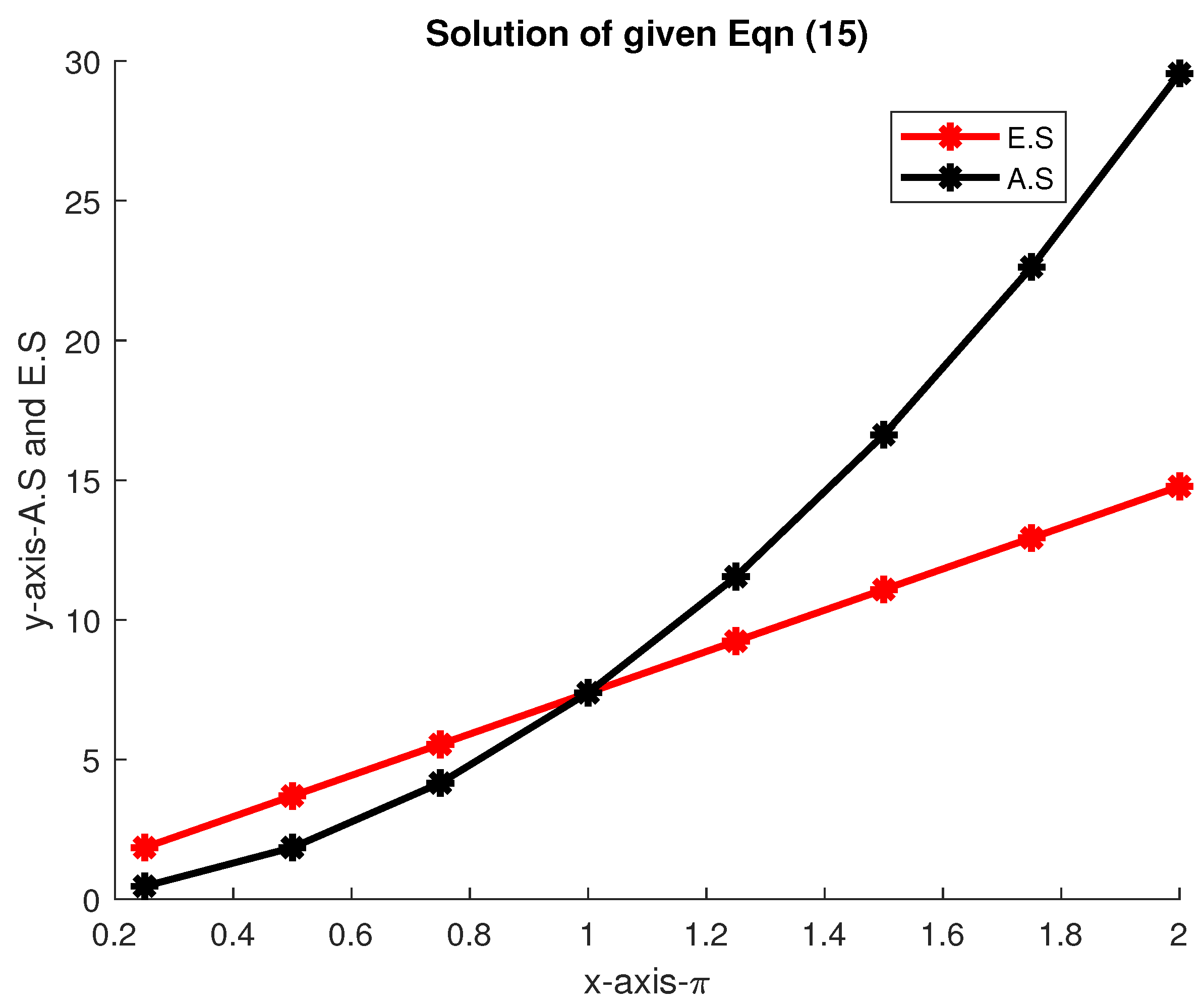
Figure 1. Prove that the fixed point of π is 1 and is unique.
Mathematics 11 04101 g001
Table 1. Numerical results for Example 4.
π e 2 π π e 2 π Error
0.251.84730.46181.0112
0.503.69451.84731.8473
0.755.54184.15631.3855
1.007.38917.38910.0000
1.259.236311.54542.3091
1.5011.083616.62545.5418
1.7512.930822.62899.6981
2.0014.778129.556214.7781
Disclaimer/Publisher’s Note: The statements, opinions and data contained in all publications are solely those of the individual author(s) and contributor(s) and not of MDPI and/or the editor(s). MDPI and/or the editor(s) disclaim responsibility for any injury to people or property resulting from any ideas, methods, instructions or products referred to in the content.

