A Numerical Approach for Dealing with Fractional Boundary Value Problems

Abstract

This paper proposes a novel numerical approach for handling fractional boundary value problems. Such an approach is established on the basis of two numerical formulas; the fractional central formula for approximating the Caputo differentiator of order $\alpha$ and the fractional central formula for approximating the Caputo differentiator of order $2\alpha$, where $0<\alpha \le 1$. The first formula is recalled here, whereas the second one is derived based on the generalized Taylor theorem. The stability of the proposed approach is investigated in view of some formulated results. In addition, several numerical examples are included to illustrate the efficiency and applicability of our approach.

1. Introduction

The significance of fractional differential equations (FDEs) has grown significantly in recent decades. This is, of course, due to their value in modeling various phenomena in many practical and industrial applications such as science, physics, dynamics, mechanics, engineering, etc. When dealing with ordinary/partial differential equations, one might be concerned about obtaining solutions to these equations so that they satisfy specific conditions [1,2]. In general, we will have initial conditions once certain conditions are provided at a single point of an independent variable, whereas we will have boundary conditions once the conditions are provided at more than a single point of that variable. Actually, obtaining a solution of a fractional-order problem in accordance with n-boundary conditions is called an FBVP. Such a problem in its linear and $2\alpha$-order cases is regarded as a very important problem due to its various applications in technology and science. In this work, two boundary conditions are typically assumed at end points of an interval, as in most physical applications. In particular, we consider the following FBVP:

$$p{D}^{2\alpha }y\left(x\right)+q{D}^{\alpha }y\left(x\right)+ry\left(x\right)=f\left(x\right),$$

(1)

subject to the boundary conditions

$$y\left(a\right)=y_{a}y\left(b\right)=y_b,a<x<b,$$

(2)

where $p,q,r$ are constants and $0<\alpha \le 1$ and $y_a,y_b$ are given real numbers.

The boundary value problems consisting of FDEs have contributed to a deep understanding of many processes in different sciences, as different types of these equations can be solved using certain mathematical methods which meet specific boundary conditions. Given the impossibility of solving nonlinear types of the BVPs analytically, several numerical approaches are used, see [3,4,5,6,7]. It should be noted that the finite difference method can provide very good numerical solutions for different types of FDES, see, e.g., [8,9,10]. From this point of view, we here propose to use the fractional central formula for approximating the Caputo differentiator of order $\alpha$ established in [11], and another formula called the fractional central formula for approximating the Caputo differentiator of order $2\alpha$, to find approximate solutions to a type of FBVPs given in (1), where $0<\alpha \le 1$. The stability of the proposed method is then examined, and several numerical examples are provided for completeness.

This paper is coordinated as follows. In Section 2, necessary preliminaries and some properties connected with fractional calculus are presented. Section 3 displays the methodology of the proposed method coupled with its stability. Section 4 provides a number of examples with some figures and tabulated results attached to illustrate the fulfilled findings. Section 5 finishes this work by declaring a conclusion.

2. Preliminaries

In this section, we mention some basic and necessary definitions in fractional calculus, such as the Riemann–Liouville integral and derivative, the Caputo derivative, and properties of the operators, which will be applied throughout the paper.

Definition 1

([12,13]). The Riemann–Liouville fractional integral of the function f of order γ is outlined as

$${\mathcal{J}}^{\gamma }f\left(t\right)=\frac{1}{\mathsf{\Gamma }\left(\gamma \right)}{\int }_0^t{(t-\tau )}^{\gamma -1}f\left(\tau \right)d\tau ,$$

(3)

where $t>0$ and $0<\gamma \le 1$.

Remark 1

([12,13]). It is useful to mention some characteristics of the Riemann–Liouville integral operator, which are listed below for completeness:

• The identity property, i.e.,

  $${\mathcal{J}}^{0}f\left(t\right)=f\left(t\right).$$

  (4)
• The power rule property, i.e.,

  $${\mathcal{J}}^{\gamma }{t}^m=\frac{\mathsf{\Gamma }(m+1)}{\mathsf{\Gamma }(m+\gamma +1)}{t}^{m+\gamma },m\in {\mathbb{Z}}^{+}.$$

  (5)
• The commutation property, i.e.,

  $${\mathcal{J}}^{\gamma }{\mathcal{J}}^{\mathcal{B}}f\left(t\right)={\mathcal{J}}^{\gamma +\mathcal{B}}f\left(t\right)={\mathcal{J}}^{\mathcal{B}}{\mathcal{J}}^{\gamma }f\left(t\right),\gamma ,\mathcal{B}\ge 0.$$

  (6)

Definition 2

([12,13]). Let $n-1<\gamma \le n$ such that n is a positive integer and $\gamma \in {\mathbb{R}}^{+}$. The Riemann–Liouville derivative of fractional-order γ is outlined as

$$D^{\gamma }f\left(t\right)=\frac{1}{\mathsf{\Gamma }(n-\gamma )}\frac{d^n}{d{t}^n}{\int }_0^t\frac{f^{\left(n\right)}\left(\tau \right)}{{(t-\tau )}^{\gamma +1-n}}d\tau .$$

(7)

Definition 3

([12,13]). The Caputo fractional differential operator of order γ is outlined as

$$D^{\gamma }f\left(x\right)=\frac{1}{\mathsf{\Gamma }(n-\gamma )}{\int }_0^t\frac{f^{\left(n\right)}\left(\tau \right)}{{(t-\tau )}^{\gamma +1-n}}d\tau ,$$

(8)

where $t>0$ and $n-1<\gamma \le n$ such that $n\in \mathbb{N}$.

Remark 2

([12,13]). The Caputo fractional derivative satisfies the following properties:

• The power rule property, i.e.,

  $$D^{\gamma }{t}^{\epsilon }=\left\{\begin{array}{cc}\frac{\mathsf{\Gamma }(\epsilon +1)}{\mathsf{\Gamma }(\epsilon -\gamma +1)}{t}^{\epsilon -\gamma },& n-1<\alpha <n,\epsilon >n-1,\epsilon \in \mathbb{R}\\ 0,& n-1<\alpha <n,\epsilon \le n-1,\epsilon \in \mathbb{N}\end{array}\right..$$

  (9)
• The constant property, i.e.,

  $$D^{\gamma }c=0,$$

  (10)

  where c is constant.
• Interpolation property, i.e.,

  $$\underset{\gamma \to n}{lim}{D}^{\gamma }f\left(t\right)=D^{n}f\left(t\right).$$

  (11)
• Linearity property, i.e.,

  $$D^{\gamma }({\lambda }_{1}f\left(t\right)+{\lambda }_{2}g\left(t\right))={\lambda }_1{D}^{\gamma }f\left(t\right)+{\lambda }_2{D}^{\gamma }g\left(t\right),$$

  (12)

  where ${\lambda }_1$ and ${\lambda }_2$ are two constants.
• Non-commutation property, i.e.,

  $$D^{\gamma }{D}^{\mu }f\left(t\right)\ne D^{\mu }{D}^{\gamma }f\left(t\right),$$

  (13)

  where $n-1<\gamma ,\mu \le$ n such that $n\in \mathbb{N}$.

Theorem 1

([14]). Suppose that $D^{k\alpha }f\left(x\right)\in C^{n+1}(0,b]$ for $k=0,1,\cdots ,n+1,$ where $0<\alpha \le 1$. Then, the function f can be expanded about $x=x_0$ as follows:

$$\begin{array}{c}\hfill f\left(x\right)=\sum _{i=0}^n\frac{{(x-x_0)}^{i\alpha }}{\mathsf{\Gamma }(i\alpha +1)}{D}^{i\alpha }f\left(x_0\right)+\frac{{(x-x_0)}^{(n+1)\alpha }}{\mathsf{\Gamma }\left(\right(n+1)\alpha +1)}{D}^{(n+1)\alpha }f\left(\xi \right),\end{array}$$

(14)

where $0<\xi <b$ and $x\in (0,b]$.

3. Methodology and Stability

In this section, we attempt to develop a novel numerical approach to deal with FBVPs. This approach is accomplished based upon a recent formula established in [11] called the fractional central formula for approximating the Caputo differentiator of order $\alpha$, and another formula called the fractional central formula for approximating the Caputo differentiator of order $2\alpha$, which would be established here, where $0<\alpha \le 1$. But before all of this, we recall below the first formula by stating the following theorem.

Theorem 2

([11]). Let $f\in C^3(0,b]$ and $x_0,x_1,x_3$ be three distinct points in the interval $(0,b]$ such that $0=x_0<x_1=x_0+$$h<x_2=x_0+2h=b$, where $h>0$. Then, for any $x\in (0,b]$, the fractional central formula for approximating the Caputo differentiator of order α is determined by

$$\begin{array}{cc}\hfill D_t^{\alpha }f\left(x\right)=& \frac{x^{2-\alpha }}{h^{2\alpha }\mathsf{\Gamma }(3-\alpha )}\left(f\left(x_0\right)-2f\left(x_1\right)+f\left(x_2\right)\right)\hfill \\ \hfill & -\frac{x^{1-\alpha }}{2h^{2\alpha }\mathsf{\Gamma }(2-\alpha )}\left(f\left(x_0\right)(x_1+x_2)-2f\left(x_1\right)(x_0+x_2)+f\left(x_2\right)(x_0+x_1)\right)\hfill \\ \hfill & +{\displaystyle \frac{f^{\left(3\right)}\left(\xi \right)}{6}}\left(\frac{6}{\mathsf{\Gamma }(4-\alpha )}{x}^{3-\alpha }-\frac{2(x_0+x_1+x_2)}{\mathsf{\Gamma }(3-\alpha )}{x}^{2-\alpha }+\frac{(x_0{x}_1+x_0{x}_2+x_1{x}_2)}{\mathsf{\Gamma }(2-\alpha )}{x}^{1-\alpha }\right),\hfill \end{array}$$

(15)

where $0<\alpha \le 1$, for an unknown $\xi \in (0,b)$.

3.1. Approximating Caputo Differentiator of Order $2\alpha$

Herein, on the basis of the generalized Taylor Theorem 1, we intend to derive a novel formula called the fractional central formula for approximating the Caputo differentiator of order $2\alpha$, where $0<\alpha \le 1$.

Theorem 3.

Suppose that $f\in C^4(0,b]$ and $x_0,x_1,x_2$ are distinct points in the interval $(0,b]$ such that $0=x_0<x_1=x_0+h<x_2=x_0+2h=b$ with $h>0$. Let $0<\alpha \le 1$, then the fractional central formula for approximating the Caputo differentiator of order $2\alpha$ is determined by

$$D^{2\alpha }f\left(x\right)=\frac{\mathsf{\Gamma }(2\alpha +1)}{2h^{2\alpha }}\left(f\left(x_0\right)-2f\left(x_1\right)+f\left(x_2\right)\right)-\frac{\mathsf{\Gamma }(2\alpha +1)}{\mathsf{\Gamma }(4\alpha +1)}{h}^{2\alpha }{D}^{4\alpha }f\left(\xi \right),$$

(16)

where $x\in (0,b)$ for an unknown $\xi \in (0,b)$.

Proof. 

To prove this result, we first expand the function f about $x_0$ using Theorem 1 to obtain

$$f\left(x\right)=f\left(x_0\right)+\frac{{(x-x_0)}^{\alpha }}{\mathsf{\Gamma }(\alpha +1)}{D}^{\alpha }f\left(x_0\right)+\frac{{(x-x_0)}^{2\alpha }}{\mathsf{\Gamma }(2\alpha +1)}{D}^{2\alpha }f\left(x_0\right)+\frac{{(x-x_0)}^{3\alpha }}{\mathsf{\Gamma }(3\alpha +1)}{D}^{3\alpha }f\left(x_0\right)+\frac{{(x-x_0)}^{4\alpha }}{\mathsf{\Gamma }(4\alpha +1)}{D}^{4\alpha }f\left({\xi }_1\right).$$

(17)

Consequently, we can approximate the function f at $x_1=x_0+h$. In other words, we can have

$$f(x_0+h)=f\left(x_0\right)+\frac{h^{\alpha }}{\mathsf{\Gamma }(\alpha +1)}{D}^{\alpha }f\left(x_0\right)+\frac{h^{2\alpha }}{\mathsf{\Gamma }(2\alpha +1)}{D}^{2\alpha }f\left(x_0\right)+\frac{h^{3\alpha }}{\mathsf{\Gamma }(3\alpha +1)}{D}^{3\alpha }f\left(x_0\right)+\frac{h^{4\alpha }}{\mathsf{\Gamma }(4\alpha +1)}{D}^{4\alpha }f\left({\xi }_1\right).$$

(18)

From this point of view, we can use the transform variables for both $x_0$ and $x_1=x_0+h$ to be x and $x+h$, respectively. This would immediately give

$$f(x+h)=f\left(x\right)+\frac{h^{\alpha }}{\mathsf{\Gamma }(\alpha +1)}{D}^{\alpha }f\left(x\right)+\frac{h^{2\alpha }}{\mathsf{\Gamma }(2\alpha +1)}{D}^{2\alpha }f\left(x\right)+\frac{h^{3\alpha }}{\mathsf{\Gamma }(3\alpha +1)}{D}^{3\alpha }f\left(x\right)+\frac{h^{4\alpha }}{\mathsf{\Gamma }(4\alpha +1)}{D}^{4\alpha }f\left({\xi }_1\right).$$

(19)

In a similar manner, we can get

$$f(x-h)=f\left(x\right)-\frac{h^{\alpha }}{\mathsf{\Gamma }(\alpha +1)}{D}^{\alpha }f\left(x\right)+\frac{h^{2\alpha }}{\mathsf{\Gamma }(2\alpha +1)}{D}^{2\alpha }f\left(x\right)-\frac{h^{3\alpha }}{\mathsf{\Gamma }(3\alpha +1)}{D}^{3\alpha }f\left(x\right)+\frac{h^{4\alpha }}{\mathsf{\Gamma }(4\alpha +1)}{D}^{4\alpha }f\left({\xi }_{-1}\right),$$

(20)

where $x-h<{\xi }_{-1}<x<{\xi }_1<x+h$. Adding (19) to (20) yields

$$f(x+h)+f(x-h)=2f\left(x\right)+\frac{2h^{2\alpha }}{\mathsf{\Gamma }(2\alpha +1)}{D}^{2\alpha }f\left(x\right)+\frac{h^{4\alpha }}{\mathsf{\Gamma }(4\alpha +1)}\left(D^{4\alpha }f\left({\xi }_1\right)+D^{4\alpha }f\left({\xi }_{-1}\right)\right).$$

(21)

Now, due to $\frac{1}{2}\left(D^{4\alpha }f\left({\xi }_1\right)+D^{4\alpha }f\left({\xi }_{-1}\right)\right)$ lying between $D^{4\alpha }f\left({\xi }_1\right)$ and $D^{4\alpha }f\left({\xi }_{-1}\right)$, by the Intermediate Value Theorem we can infer that $\xi$ exists between ${\xi }_1$ and ${\xi }_1$, and so in $(x-h,x+h)$. Thus, we have

$$D^{4\alpha }f\left(\xi \right)=\frac{1}{2}\left(D^{4\alpha }f\left({\xi }_1\right)+D^{4\alpha }f\left({\xi }_{-1}\right)\right).$$

This consequently implies

$$\frac{\mathsf{\Gamma }(2\alpha +1)}{2h^{2\alpha }}(f(x-h)-2f\left(x\right)+f(x+h))=D^{2\alpha }f\left(x\right)+\frac{\mathsf{\Gamma }(2\alpha +1)}{\mathsf{\Gamma }(4\alpha +1)}{h}^{2\alpha }{D}^{4\alpha }f\left(\xi \right),$$

(22)

which immediately gives the desired result. □

Remark 3.

It is obvious that, if we take $\alpha =1$ in formula (16), then the conventional second derivative midpoint formula will be immediately yielded.

3.2. Analysis of the Method

At the beginning of this section, we intend to depict the procedure of solving the FBVP given in (1) and (2). For this purpose, we apply Theorems 2 and 3 to approximate $D^{\alpha }y\left(x\right)$ and $D^{2\alpha }y\left(x\right)$, respectively. In other words, we have

$$D^{\alpha }y\left(x\right)\approx \frac{x_1^{2-\alpha }}{h^{2\alpha }\mathsf{\Gamma }(3-\alpha )}\left(y\left(x_0\right)-2y\left(x_1\right)+y\left(x_2\right)\right)$$

(23)

and

$$D^{2\alpha }y\left(x\right)\approx \frac{\mathsf{\Gamma }(2\alpha +1)}{2h^{2\alpha }}\left(y\left(x_0\right)-2y\left(x_1\right)+y\left(x_2\right)\right),$$

(24)

where $h,x_0,x_1,x_2$ are defined previously in Theorem 3, and $0<\alpha \le 1$. For the purpose of developing a novel approach to find the solution of the problem (1) and (2), we divide the interval $[a,b]$ into n subintervals through $x_i=a+ih$, for $i=0,1,2,\dots ,N$, such that $a=x_0$ and $b=x_n$, where $h=\frac{b-a}{N}$. Now, at the point $x=x_i$, we have

$$D^{\alpha }y\left(x_i\right)\approx \frac{{x_i}^{2-\alpha }}{h^{2\alpha }\mathsf{\Gamma }(3-\alpha )}\left(y\left(x_{i-1}\right)-2y\left(x_i\right)+y\left(x_{i+1}\right)\right),$$

(25)

and

$$D^{2\alpha }y\left(x_i\right)\approx \frac{\mathsf{\Gamma }(2\alpha +1)}{2h^{2\alpha }}\left(y\left(x_{i-1}\right)-2y\left(x_i\right)+y\left(x_{i+1}\right)\right),$$

(26)

for $i=1,2,\dots ,N$. By substituting (25) and (26) in (1), we get

$$\frac{\mathsf{\Gamma }(2\alpha +1)}{2h^{2\alpha }}(y\left(x_{i-1}\right)-2y\left(x_i\right)+y\left(x_{i+1}\right))+\frac{q{x_i}^{2-\alpha }}{h^{2\alpha }\mathsf{\Gamma }(3-\alpha )}(y\left(x_{i-1}\right)-2y\left(x_i\right)+y\left(x_{i+1}\right))+ry\left(x_i\right)=f\left(x_i\right),$$

(27)

for $i=1,2,\dots ,N$. Actually, formula (27) can be rewritten in the form

$$\begin{array}{cc}\hfill \left(\frac{\mathsf{\Gamma }(2\alpha +1)}{2}+\frac{q{x_i}^{2-\alpha }}{\mathsf{\Gamma }(3-\alpha )}\right)y\left(x_{i-1}\right)& -\left(\mathsf{\Gamma }(2\alpha +1)+\frac{2q{x_i}^{2-\alpha }}{\mathsf{\Gamma }(3-\alpha )}+r\right)y\left(x_i\right)\hfill \\ \hfill & +\left(\frac{\mathsf{\Gamma }(2\alpha +1)}{2}+\frac{q{x_i}^{2-\alpha }}{\mathsf{\Gamma }(3-\alpha )}\right)y\left(x_{i+1}\right)=h^{2\alpha }f\left(x_i\right),\hfill \end{array}$$

(28)

for $i=1,2,\dots ,N$. For simplicity, we set the following assumptions:

$$a_i=\frac{\mathsf{\Gamma }(2\alpha +1)}{2}+\frac{q{x}_i^{2-\alpha }}{\mathsf{\Gamma }(3-\alpha )}$$

(29)

and

$$b_i=-\left(\mathsf{\Gamma }(2\alpha +1)+\frac{2q{x}_i^{2-\alpha }}{\mathsf{\Gamma }(3-\alpha )}+r\right),$$

(30)

for $i=1,2,\dots ,N$. This immediately converts (28) to

$$a_i\left(y\left(x_{i-1}\right)+y\left(x_{i+1}\right)\right)+b_{i}y\left(x_i\right)=h^{2}f\left(x_i\right),$$

(31)

for $i=1,2,\dots ,N$. In fact, the above formulas can be expressed in the matrix form as follows:

$$\begin{array}{cc}\hfill & \left(\begin{array}{cccccccc}{b}_1& a_1& 0& 0& \dots & 0& 0& 0\\ a_2& b_2& a_2& 0& \dots & 0& 0& 0\\ 0& a_3& b_3& a_3& \dots & 0& 0& 0\\ ⋮& ⋮& ⋮& ⋮& \ddots & ⋮& ⋮& ⋮\\ 0& 0& 0& 0& \dots & a_{N-1}& b_{N-1}& a_{N-1}\\ 0& 0& 0& 0& \dots & 0& a_N& b_N\end{array}\right)\left(\begin{array}{c}{y}_1\\ y_2\\ y_3\\ ⋮\\ y_{N-1}\\ y_N\end{array}\right)=h^{2\alpha }\left(\begin{array}{c}f\left(x_1\right)\\ f\left(x_2\right)\\ f\left(x_3\right)\\ ⋮\\ f\left(x_{N-1}\right)\\ f\left(x_N\right)\end{array}\right)-\left(\begin{array}{c}{a}_1{y}_a\\ 0\\ 0\\ ⋮\\ 0\\ a_N{y}_b\end{array}\right).\hfill \end{array}$$

(32)

The above linear system can be denoted by $A\mathbf{X}=\mathbf{M}$, where

$$\begin{array}{cc}\hfill & A=\left(\begin{array}{cccccccc}{b}_1& a_1& 0& 0& \dots & 0& 0& 0\\ a_2& b_2& a_2& 0& \dots & 0& 0& 0\\ 0& a_3& b_3& a_3& \dots & 0& 0& 0\\ ⋮& ⋮& ⋮& ⋮& \ddots & ⋮& ⋮& ⋮\\ 0& 0& 0& 0& \dots & a_{N-1}& b_{N-1}& a_{N-1}\\ 0& 0& 0& 0& \dots & 0& a_N& b_N\end{array}\right)\hfill \end{array}$$

(33)

$$\mathbf{X}={\left[y_1,y_2,y_3,\cdots ,y_{N-1},y_N\right]}^T$$

and

$$\mathbf{M}={\left[h^{2\alpha }f\left(x_1\right)-a_1{y}_a,h^{2\alpha }f\left(x_2\right),h^{2\alpha }f\left(x_3\right),\cdots ,h^{2\alpha }f\left(x_{N-1}\right),h^{2\alpha }f\left(x_N\right)-a_N{y}_N\right]}^T.$$

As a matter of fact, system (32) is called tridiagonal and could be solved algebraically using the Thomas algorithm [15]. In particular, if we take formula (31) again as follows:

$$a_i\left(y_{i-1}+y_{i+1}\right)+b_i{y}_i=d_i,$$

(34)

where $d_i=h^{2\alpha }f\left(x_i\right)$ for $i=1,2,\dots ,N$. Now, formula (34) can be written in the form:

$$\begin{array}{cc}\hfill & b_1{y}_1+a_1{y}_2=d_1^{*}\hfill \\ \hfill & b_2{y}_2+a_2(y_1+y_3)=d_2\hfill \\ \hfill & b_3{y}_3+a_3(y_2+y_4)=d_3\hfill \\ \hfill & ⋮\hfill \\ \hfill & b_{N-1}{y}_{N-1}+a_{N-1}(y_{N-2}+y_N)=d_{N-1}\hfill \\ \hfill & a_N{y}_{N-1}+b_N{y}_N=d_N^{*},\hfill \end{array}$$

(35)

where $d_1^{*}=h^{2\alpha }f\left(x_1\right)-a_1{y}_a$ and $d_N^{*}=h^{2\alpha }f\left(x_N\right)-a_N{y}_b$. By considering the Thomas algorithm, we assume $b_1\ne 0$ and eliminate $y_1$ from the second equation of system (35). This gives

$$b_2^{\prime }{y}_2+a_2{y}_3=d_2^{\prime },$$

where $b_2^{\prime }=b_2-a_1\frac{a_2}{b_1}$ and $d_2^{\prime }=d_2-d_1\frac{a_2}{b_1}$. Next, assuming $b_2^{\prime }\ne 0$ and eliminating $y_2$ from the third equation of system (35) yields

$$b_3^{\prime }{y}_3+a_3{y}_4=d_3^{\prime },$$

where $b_3^{\prime }=b_3-a_2\frac{a_3}{b_2^{\prime }}$ and $d_3^{\prime }=d_3-d_2^{\prime }\frac{a_3}{b_2^{\prime }}$. Similarly, if we assume that $b_k^{\prime }\ne 0$ and eliminating $y_k$ from the $(k+1)$th-equation of the system (35), we obtain

$$b_{k+1}^{\prime }{y}_{k+1}+a_{k+1}{y}_{k+2}=d_{k+1}^{\prime },$$

where $b_{k+1}^{\prime }=b_{k+1}-a_k\frac{a_{k+1}}{b_k^{\prime }}$ and $d_{k+1}^{\prime }=d_{k+1}-d_k^{\prime }\frac{a_{k+1}}{b_k^{\prime }}$, for $k=1,2,\dots ,N-1$. Consequently, by back substituting N and assuming $b_N^{\prime }\ne 0$ in which $y_N=\frac{d_N^{\prime }}{b_N^{\prime }}$, we have

$$y_k=\frac{d_k^{\prime }-a_k{y}_{k+1}}{b_k^{\prime }},$$

for $k=N-1,N-2,\dots ,1$. This finishes the Thomas algorithm and, hence, by proper MATLAB code, we can obtain the desired numerical solution of the aimed system (1) and (2).

3.3. Stability of the Method

In order to insure of the stability of the fractional central formula for approximating the Caputo differentiator of order $2\alpha$, where $0<\alpha \le 1$, we consider the following FBVP:

$$D^{2\alpha }y\left(x\right)=f\left(x\right),$$

(36)

with the boundary conditions

$$y\left(a\right)=y_a,y\left(b\right)=y_b,$$

(37)

where $a<x<b$. The important question to be asked here is how would $\widehat{\mathbf{Y}}={[y_1,y_2,y_3,\cdots ,y_{N-1}]}^T$ be regarded a good approximation of solution of problem (36) and (37). To answer this question, we need to estimate the error in the discrete values $y_1,y_2,\dots ,y_N$ related to the true solution $y\left(x\right)$. In this regard, we assume the pointwise error is of the form $y_i-y\left(x_i\right)$, for $i=0,1,\dots ,N$, and the true vector is of the form $\mathbf{Y}={[y_1,y_2,y_3,\dots ,y_{N-1},y_N]}^T$. This gives the error of the form

$$\mathbf{E}=\widehat{\mathbf{Y}}-\mathbf{Y},$$

which contains all error at each grid point. To obtain a bound on the magnitude of the above vector error, we need to estimate $O\left(h^{2\alpha }\right)$ as $h\to 0$. To do this, we consider

$${\parallel \mathbf{E}\parallel }_{\infty }=\underset{1\le i\le 0}{max}|E_i|=\underset{1\le i\le 0}{max}|y_i-y\left(x_i\right)|,$$

which represents the largest error order in the interval $[a,b]$. Therefore, if ${\parallel \mathbf{E}\parallel }_{\infty }=O\left(h^{2\alpha }\right)$, then

$$|y_i-y\left(x_i\right)|=O\left(h^{2\alpha }\right),$$

for $i=0,1,\dots ,N$.

Next, our aim is to estimate the error in our proposed difference approach. To do so, we should be concerned with the local truncation error, and then with the stability of this approach for the purpose of justifying the boundedness of the global error. So, let us start with the local truncation error, which would be as follows:

$$T_i=\frac{\mathsf{\Gamma }(2\alpha +1)}{2h^{2\alpha }}\left(y\left(x_{i-1}\right)-2y\left(x_i\right)+y\left(x_{i+1}\right)\right)-f\left(x_i\right),$$

(38)

or

$$T_i=D^{2\alpha }y\left(x_i\right)-\frac{h^{2\alpha }\mathsf{\Gamma }(2\alpha +1)}{\mathsf{\Gamma }(4\alpha +1)}{D}^{4\alpha }y\left({\xi }_i\right)+O\left(h^{4\alpha }\right)-f\left(x_i\right),$$

(39)

for $i=1,2,\dots ,N$. Now, by using $D^{2\alpha }y\left(x\right)=f\left(x\right)$, we have

$$T_i=-\frac{h^{2\alpha }\mathsf{\Gamma }(2\alpha +1)}{\mathsf{\Gamma }(4\alpha +1)}{D}^{4\alpha }y\left({\xi }_i\right)+O\left(h^{4\alpha }\right).$$

(40)

Now, though $D^{4\alpha }y\left({\xi }_i\right)$ is unknown fixed and is independent of h, we have $T_i\sim O\left(h^{4\alpha }\right)$ as $h\to 0$. If we define $\mathbf{T}$ as a vector containing $T_i$, then

$$\mathbf{T}=A\mathbf{Y}-\mathbf{M},$$

which implies

$$A\mathbf{Y}=\mathbf{M}+\mathbf{T}.$$

(41)

Now, to address the global error, we can have from (41) the following approximation:

$$A\widehat{\mathbf{Y}}=\mathbf{M}.$$

(42)

So, the global error is defined as

$$\mathbf{E}=\widehat{\mathbf{Y}}-\mathbf{Y}.$$

Now, subtracting (41) and (42) yields

$$A\left(\widehat{\mathbf{Y}}-\mathbf{Y}\right)=-\mathbf{T},$$

or

$$A\mathbf{E}=-\mathbf{T}.$$

(43)

This implies

$$\frac{\mathsf{\Gamma }(2\alpha +1)}{2h^{2\alpha }}\left(E_{i-1}-2E_i+E_{i+1}\right)=-T\left(x_i\right),$$

(44)

with boundary conditions

$$E_0=0,E_{N+1}=0,$$

(45)

for $i=1,2,\dots ,N$. Note that problems (44) and (45) are the same as the difference equation reported previously for $y_i$, except $f\left(x_i\right)=-T\left(x_i\right)$, for $i=1,2,\dots ,N$. Actually, problems (44) and (45) can be expressed as

$$D^{2\alpha }e\left(x\right)=-\tau \left(x\right),$$

(46)

with boundary conditions

$$e\left(a\right)=0,e\left(b\right)=0,$$

(47)

where $a\le x\le b$ and

$$\tau \left(x\right)=\frac{\mathsf{\Gamma }(2\alpha +1)}{\mathsf{\Gamma }(4\alpha +1)}{D}^{4\alpha }y\left(x\right).$$

Now, if we operate ${\mathcal{J}}^{\alpha }$ in Equation (46), we get

$$D^{\alpha }e\left(x\right)=-h^{2\alpha }\frac{\mathsf{\Gamma }(2\alpha +1)}{\mathsf{\Gamma }(4\alpha +1)}(D^{3\alpha }y\left(x\right)-\left\{D^{2\alpha }\right\}y\left(0\right)),$$

or

$$D^{\alpha }e\left(x\right)=h^{2\alpha }\frac{\mathsf{\Gamma }(2\alpha +1)}{\mathsf{\Gamma }(4\alpha +1)}{D}^{2\alpha }y\left(0\right)-h^{2\alpha }\frac{\mathsf{\Gamma }(2\alpha +1)}{\mathsf{\Gamma }(4\alpha +1)}{D}^{3\alpha }y\left(x\right).$$

(48)

By operating ${\mathcal{J}}^{\alpha }$ twice again in Equation (48), we obtain

$$e\left(x\right)=h^{2\alpha }\frac{\mathsf{\Gamma }(2\alpha +1)}{\mathsf{\Gamma }(4\alpha +1)}\frac{x^{\alpha }}{\mathsf{\Gamma }(\alpha +1)}{D}^{2\alpha }y\left(0\right)-h^{2\alpha }\frac{\mathsf{\Gamma }(2\alpha +1)}{\mathsf{\Gamma }(4\alpha +1)}\left(D^{2\alpha }y\left(x\right)-D^{\alpha }y\left(0\right)\right),$$

or

$$e\left(x\right)=-h^{2\alpha }\frac{\mathsf{\Gamma }(2\alpha +1)}{\mathsf{\Gamma }(4\alpha +1)}{D}^{2\alpha }y\left(x\right)+h^{2\alpha }\frac{\mathsf{\Gamma }(2\alpha +1)}{\mathsf{\Gamma }(4\alpha +1)}\left(\frac{x^{\alpha }}{\mathsf{\Gamma }(\alpha +1)}{D}^{2\alpha }y\left(0\right)-D^{\alpha }y\left(0\right)\right).$$

This implies ${∥\mathbf{E}∥}_{\infty }\approx O\left(h^{2\alpha }\right)$, which represents the desired estimation for the global error.

Now, with aim of dealing with the stability of the proposed difference scheme, we consider again system (43) in which A is the corresponding tridiagonal matrix, $\mathbf{E}$ is the global error matrix, and $\mathbf{T}$ is the local truncation error matrix. In fact, system (43) can be rewritten as

$$A^h{\mathbf{E}}^h=-{\mathbf{T}}^h,$$

(49)

for a given $h=\frac{1}{n+1}$. It is important to mention that $A_{m\times m}^h$, and as a result the dimension of $A^h$ will grow as $h\to 0$. Now, let ${\left(A^h\right)}^{-1}$ exist. Then, we have

$${\mathbf{E}}^h=-{\left(A^h\right)}^{-1}{\mathbf{T}}^h.$$

(50)

Consequently, we obtain

$$∥{\mathbf{E}}^h∥=∥{\left(A^h\right)}^{-1}{\mathbf{T}}^h∥\le ∥{\left(A^h\right)}^{-1}∥∥{\mathbf{T}}^h∥.$$

But we have $∥{\mathbf{T}}^h∥\sim O\left(h^{2\alpha }\right)$. So, we expect the same for $∥{\mathbf{E}}^h∥$. Thus, for $∥{\mathbf{E}}^h∥\sim O\left(h^{2\alpha }\right)$, then $∥{\left(A^h\right)}^{-1}∥$ is independent of h as $h\to 0$, say $∥{\left(A^h\right)}^{-1}∥\le c$, for sufficiently small h, where c is constant. Therefore, we have

$$∥{\mathbf{E}}^h∥\le c∥{\mathbf{T}}^h∥,$$

and hence the stability is ensured.

4. Numerical Experiments

In this section, we validate our proposed numerical approach discussed in the previous section by illustrating three numerical examples including FBVPs of the forms (1) and (2). We use MATLAB-2020 software to simulate the results in a few fractional-order values.

Example 1.

Consider the following FBVP:

$$D^{2\alpha }y+2y=0,$$

(51)

with boundary conditions

$$y\left(0\right)=1,y\left(\pi \right)=0.$$

(52)

The exact solution for problems (51) and (52) is of the form

$$y\left(x\right)=cos\left(\sqrt{2}x\right)-cot\left(\sqrt{2}\pi \right)sin\left(\sqrt{2}x\right).$$

(53)

In order to validate such an approach in handling the FBVPs, we track the proposed numerical approach discussed in Section 3. This would provide us with several approximate solutions for problem (51) and (52) with different fractional-order values, i.e., $\alpha =1,0.8,0.6,0.4$. Some of these approximate solutions are plot and compared with the exact solution (53) as can be seen in Figure 1 and

Table 1. Exact solution vs. numerical solutions of problems (51) and (52) for $\alpha =1,0.8,0.6,0.4$.

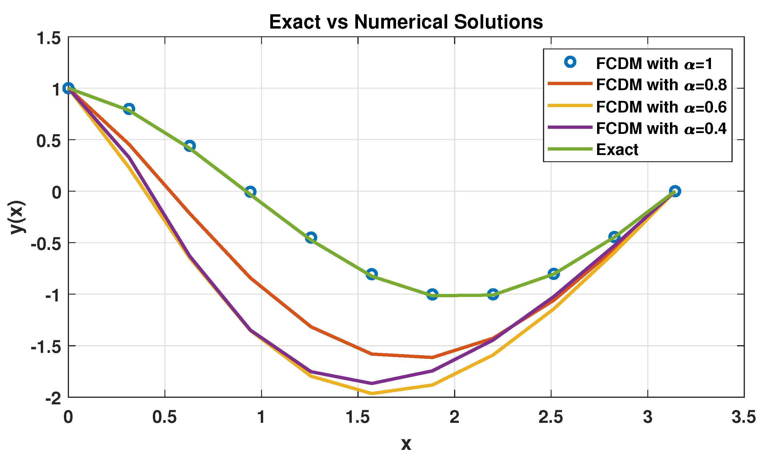
x	$\mathit{\alpha }=0.4$	$\mathit{\alpha }=0.6$	$\mathit{\alpha }=0.8$	$\mathit{\alpha }=1$	Exact Solution
0	1.0000	1.0000	1.0000	1.0000	1.0000
0.1	0.3280	0.2289	0.4551	0.7989	0.7842
0.2	−0.6303	−0.6484	−0.2165	0.4401	0.4161
0.3	−1.3491	−1.3529	−0.8424	−0.0056	−0.0328
0.4	−1.7529	−1.7965	−1.3172	−0.4501	−0.4753
0.5	−1.8669	−1.9651	−1.5815	−0.8058	−0.8255
0.6	−1.7447	−1.8819	−1.6146	−1.0025	−1.0154
0.7	−1.4452	−1.5903	−1.4282	−1.0013	−1.0082
0.8	−1.0235	−1.1431	−1.0593	−0.8024	−0.8052
0.9	−0.5283	−0.5954	−0.5622	−0.4451	−0.4459
1.0	0.0000	0.0000	0.0000	0.0000	0.0000

.

In light of the previous numerical results, one can clearly observe that the approximate solutions generated by our approach converge to the exact solution as α gets closer to 1, confirming the validity of the proposed method.

Example 2.

Consider the following FBVP:

$$D^{2\alpha }y=y+x,$$

(54)

with boundary conditions

$$y\left(0\right)=0,y\left(1\right)=0.$$

(55)

The exact solution for problems (54) and (55) is of the form

$$y\left(x\right)=\frac{sinhx}{sinh1}-x.$$

(56)

With the aim of verifying the correctness of our proposed technique in handling the FBVPs, we follow the same manner used in Example 1 coupled with using the numerical approach discussed in the previous section. This would provide us with several approximate solutions for problems (54) and (55) with different fractional-order values, i.e., $\alpha =1,0.8,0.6,0.4$. Some of these approximate solutions are plotted and compared with the exact solution (56) as can be seen in Figure 2 and

Table 2. Exact solution vs. numerical solutions of problems (54) and (55) for $\alpha =1,0.8,0.6,0.4$.

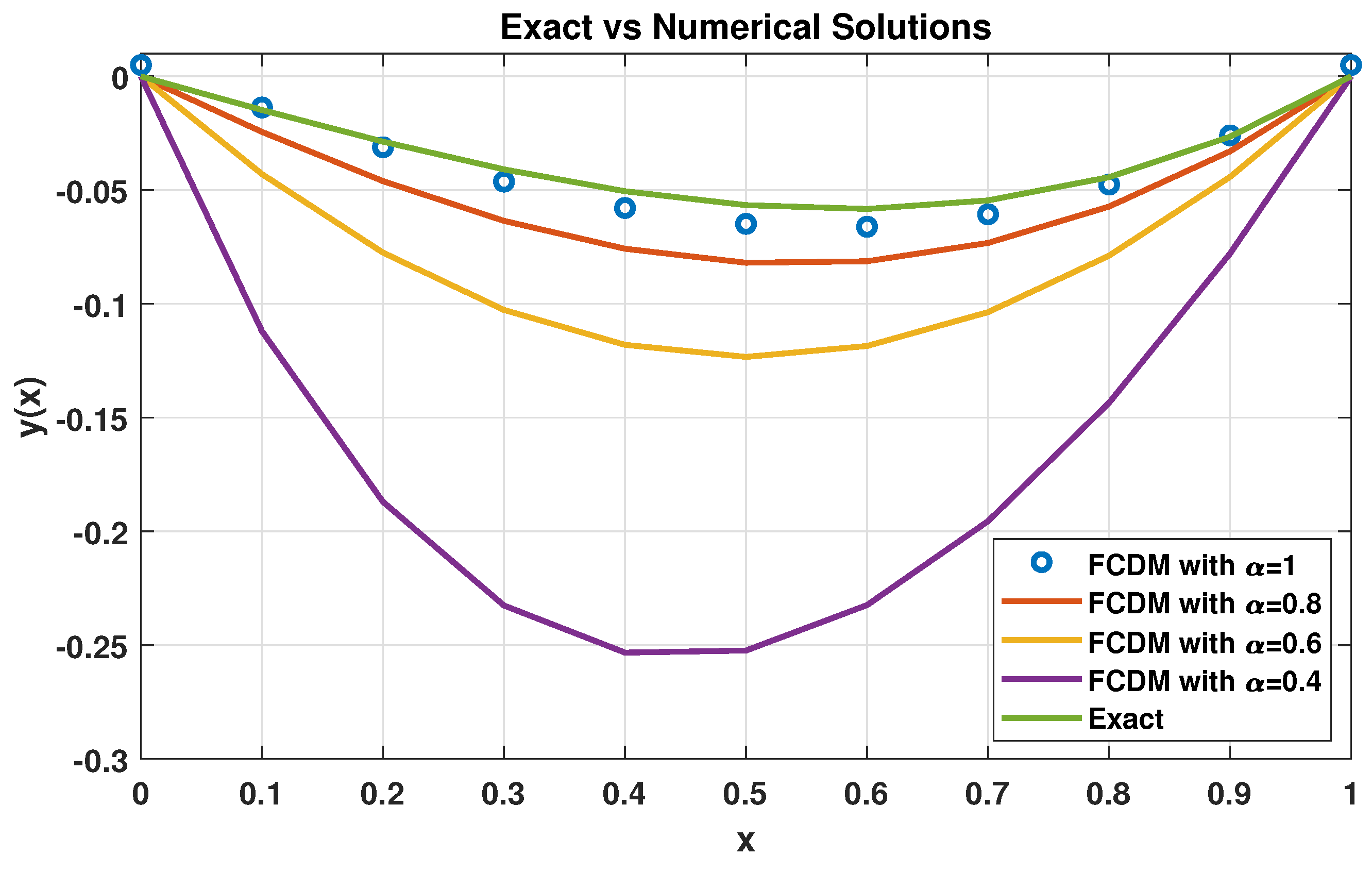
x	$\mathit{\alpha }=0.4$	$\mathit{\alpha }=0.6$	$\mathit{\alpha }=0.8$	$\mathit{\alpha }=1$	Exact Solution
0	0.0000	0.0000	0.0000	0.0000	0.0000
0.1	−0.1120	−0.0429	−0.0244	−0.0150	−0.0148
0.2	−0.1870	−0.0775	−0.0460	−0.0299	−0.0287
0.3	−0.2326	−0.1026	−0.0635	−0.0412	−0.0409
0.4	−0.2533	−0.1180	−0.0758	−0.0508	−0.0505
0.5	−0.2524	−0.1233	−0.0819	−0.0568	−0.0566
0.6	−0.2324	−0.1185	−0.0813	−0.0589	−0.0583
0.7	−0.1955	−0.1036	−0.0732	−0.566	−0.0545
0.8	−0.1435	−0.0788	−0.0572	−0.0476	−0.0443
0.9	−0.0778	−0.0442	−0.0329	−0.0269	−0.0265
1.0	0.0000	0.0000	0.0000	0.0000	0.0000

.

Herein, we can also notice that the approximate solutions generated by our numerical scheme converge to the exact solution as α gets closer to 1.

Example 3.

Consider the following FBVP:

$$D^{2\alpha }y+5D^{\alpha }y+4y=1,$$

(57)

with boundary conditions

$$y\left(0\right)=0,y\left(1\right)=0.$$

(58)

The exact solution for problems (57) and (58) is of the form

$$y\left(x\right)=\left(\frac{e^{-3}-e}{4(1-e^{-3})}\right)e^{-x}+\left(-\frac{1}{4}-\left(\frac{e^{-3}-e}{4(1-e^{-3})}\right)\right)e^{-4x}+\frac{1}{4}.$$

(59)

In a similar manner to the previous two examples, we generate here several approximate solutions for problems (57) and (58) with different fractional-order values, i.e., $\alpha =1,0.8,0.6,0.4$. Some of these approximate solutions are plotted and compared with the exact solution (59) as can be seen in Figure 3 and

Table 3. Exact solution vs. numerical solutions of problems (57) and (58) for $\alpha =1,0.8,0.6,0.4$.

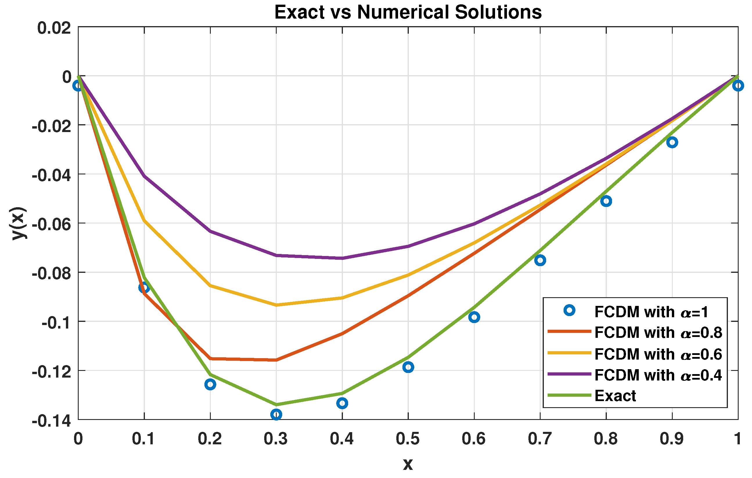
x	$\mathit{\alpha }=0.4$	$\mathit{\alpha }=0.6$	$\mathit{\alpha }=0.8$	$\mathit{\alpha }=1$	Exact Solution
0	0.0000	0.0000	0.0000	0.0000	0.0000
0.1	−0.1365	−0.0409	−0.0591	−0.0862	−0.0822
0.2	−0.1479	−0.0633	−0.0855	−0.1257	−0.1217
0.3	−0.1323	−0.0732	−0.0934	−0.1379	−0.1339
0.4	−0.1120	−0.0743	−0.0905	−0.1333	−0.1293
0.5	−0.0919	−0.0695	−0.0811	−0.1188	−0.1146
0.6	−0.0727	−0.0603	−0.0680	−0.0981	−0.0943
0.7	−0.0542	−0.0481	−0.0527	−0.0752	−0.0712
0.8	−0.0360	−0.0336	−0.0359	−0.0510	−0.0470
0.9	−0.0180	−0.0175	−0.0183	−0.0271	−0.0231
1.0	0.0000	0.0000	0.0000	0.0000	0.0000

.

Note that the approximate solutions obtained by the proposed scheme also converge to the exact solution as α gets closer to 1.

5. Conclusions

In this paper, a novel numerical approach has been successfully proposed to deal with fractional boundary value problems. This has been carried out by utilizing two numerical formulas—the fractional central formula for approximating the Caputo differentiator of order $\alpha$ and the fractional central formula for approximating the Caputo differentiator of order $2\alpha$, where $0<\alpha \le 1$. The stability analysis of the proposed approach has been discussed, and several numerical examples have been illustrated to show the applicability of the proposed method. Thus, in light of this study, we believe that we can address many other kinds of fractional-order problems in a similar manner, such as the fractional-order system of differential equations, fractional partial differential equations, and fractional integrodifferential equations. This is left to the future for further consideration.

References

- Aydemir, K.; Olǧar, H.; Mukhtarov, O.S.; Muhtarov, F.S. Differential Operator Equations with Interface Conditions in Modified Direct Sum Spaces. Filomat 2018, 32, 921–931. [Google Scholar] [CrossRef]
- Bezziou, M.; Dahmani, Z.; Jebril, I.; Belhamiti, M.M. Solvability for a Differential System of Duffing Type Via Caputo-Hadamard Approach. Appl. Math. Inf. Sci. 2022, 16, 341–352. [Google Scholar]
- Abu-Zaid, I.T.; El-Gebeily, M.A. A finite-difference method for the spectral approximation of a class of singular two-point boundary value problems. IMA J. Numer. Anal. 1994, 14, 545–562. [Google Scholar] [CrossRef]
- Fulton, C.T. Two-point boundary value problems with eigenvalue parameter contained in the boundary conditions. Proc. Roy. Soc. Edinb. 1977, 77A, 293–308. [Google Scholar] [CrossRef]
- Mukhtarov, O.; Olǧar, H.; Aydemir, K. Resolvent Operator and Spectrum of New Type Boundary Value Problems. Filomat 2015, 29, 1671–1680. [Google Scholar] [CrossRef]
- Keller, H.B. Numerical Methods for Two-Point Boundary-Value Problems; Courier Dover Publications: Mineola, NY, USA, 2018. [Google Scholar]
- Endeshaw, B. Finite Difference Method for Boundary Value Problems in Ordinary Differential Equations. Math. Theory Model. 2019, 9, 17–27. [Google Scholar]
- Zhang, T.; Li, Y. Exponential Euler scheme of multi-delay Caputo–Fabrizio fractional-order differential equations. Appl. Math. Lett. 2022, 124, 107709. [Google Scholar] [CrossRef]
- Albadarneh, R.B.; Batiha, I.M.; Zurigat, M. Numerical solutions for linear fractional differential equations of order 1 < α < 2 using finite difference method (FFDM). Int. J. Math. Comput. Sci. 2016, 16, 103–111. [Google Scholar]
- Albadarneh, R.B.; Zerqat, M.; Batiha, I.M. Numerical solutions for linear and non-linear fractional differential equations. Int. J. Pure Appl. Math. 2016, 106, 859–871. [Google Scholar] [CrossRef]
- Batiha, I.M.; Alshorm, S.; Ouannas, A.; Momani, S.; Ababneh, O.Y.; Albdareen, M. Modified Three-Point Fractional Formulas with Richardson Extrapolation. Mathematics 2022, 10, 3489. [Google Scholar] [CrossRef]
- Kilbas, A.A. Theory and Application of Fractional Differential Equations; Elsevier: Amsterdam, The Netherlands, 2006. [Google Scholar]
- Mainardi, F. Fractional Calculus. In Fractals and Fractional Calculus in Continuum Mechanics; Springer: Berlin, Germany, 1997; pp. 291–348. [Google Scholar]
- Odibat, Z.M.; Momani, S. An algorithm for the numerical solution of differential equations of fractional order. J. Appl. Math. Inform. 2008, 26, 15–27. [Google Scholar]
- Bittelli; Marco; Campbell, G.S.; Tomei, F. Soil Physics with Python: Transport in the Soil–Plant–Atmosphere System; Oxford Academic: Oxford, UK, 2015. [Google Scholar] [CrossRef]