Intelligent Fault Diagnosis of Robotic Strain Wave Gear Reducer Using Area-Metric-Based Sampling

Abstract

The main challenge with rotating machine fault diagnosis is the condition monitoring of machines undergoing nonstationary operations. One possible way of efficiently handling this situation is to use the deep learning (DL) method. However, most DL methods have difficulties when the issue of imbalanced datasets occurs. This paper proposes a novel framework to mitigate this issue by developing an area-metric-based sampling method. In the proposed process, the new sampling scheme can identify which locations of the datasets can potentially have a high degree of surprise. The basic idea of the proposed method is whenever significant deviations from the area metrics are observed to populate more sample points. In addition, to improve the training accuracy of the DL method, the obtained sampled datasets are transformed into a continuous wavelet transform (CWT)-based scalogram representing the time–frequency component. The dilated convolutional neural network (CNN) is also introduced as a classification process with the altered images. The efficacy of the proposed method is demonstrated with fault diagnosis problems for welding robots. The obtained results are also compared with existing methods.

1. Introduction

In intelligent manufacturing industrial systems, robots are widely used to autonomously carry out tasks. However, their long-term and continuous operation cause malfunctions in subcomponents, such as gears and bearings. If maintenance is not promptly carried out, these malfunctions can create various failures in the system. These failures can affect productivity and increase the probability of a shutdown. At this point, preventive maintenance of industrial machinery is a common procedure to improve the reliability and safety of the equipment. This eliminates unnecessary maintenance procedures, significantly reducing operating costs, while revitalizing research on “condition-based maintenance”. Recently, vibration signal-based condition monitoring (CM) has been commonly used for system health monitoring [1]. However, vibration signal-based CM needs additional sensors for complicated data acquisition systems and is only suitable for large electric machines [2].

In modern industrial systems, the motor current signal can be easily acquired with a current transformer that is part of the protection system, and current-based monitoring can be performed remotely from the motor control center. However, robots operate under various operating and load conditions in the industry, resulting in nonstationary current signals. Several CM technologies have been developed to detect faults in the nonstationary system. Fault diagnosis methods typically include model-based methods and data-driven methods. Data-driven models are more suitable for diagnosing systems with complex signals, because unlike model-based methods, they do not require signal patterns and error mechanisms [3]. Machine learning (ML) algorithms, such as artificial neural networks (ANNs), support vector machines (SVMs), principal component analysis (PCA), and K-nearest neighbor (KNN), have been applied to data-driven methods [4,5,6]. However, ML algorithms rely on human-engineered features to train, which can lead to inaccurate classification results [7]. Research on deep learning (DL)-based methods is actively being conducted to achieve much better accuracy under various operating conditions. Because DL is based on distributed feature learning, it can automatically learn correlations and characteristics among data, eliminating the need for feature engineering processes. However, autonomous learning of these features requires massive amounts of data.

Recently, many studies have been actively carried out to overcome the problem of data imbalance and data shortage through data augmentation. In real-world image augmentation techniques, image classification through DL includes image enlargement and reduction, rotation, and flipping [8,9,10]. For the time series, data augmentation techniques include window warping, magnitude warping, cropping, generative adversarial networks (GANs), and seasonal and trend decomposition using loess (STL) [11,12,13,14]. However, in the data augmentation methods mentioned above, the augmented data highly depend on specific input data and may not reflect the physical meaning of the original data. In previous studies, deep learning has provided excellent prediction and classification performance. However, it is impossible to interpret the model’s internal parameters for the results. If model analysis and explanation are not possible, it is difficult to convince engineers and other stakeholders, because it is challenging to present a rationale for the premaintenance and management schedule through system condition monitoring [15]. In this study, the challenges of data imbalance and shortage are addressed by enhancing the model’s reliability using a minimal number of samples through the area-metric-based sampling method. This approach involves a systematic sampling technique based on geometric characteristics within the gear mechanism. This method ensures that the augmented data maintain the physical essence of the original data, allowing for a more accurate representation. Subsequently, a specialized fault diagnosis approach using convolutional neural networks (CNNs) tailored for nonstationary systems is applied. Notably, this strategy not only improves the model’s interpretability but also facilitates a clear explanation of the results using explainable artificial intelligence (XAI).

The remainder of this paper is structured as follows: Section 2 introduces prior studies on ML- and DL-based fault diagnosis, data imbalance and data shortage problems, and XAI. Section 3 introduces the proposed intelligent fault diagnosis of the robotic strain wave gear reducer, while Section 4 describes the experiment in detail. Section 5 discusses robotic strain wave gear reducer fault diagnosis to verify the proposed method and interpret the results as XAI, and Section 6 then concludes this work.

2. Related Work

This section will provide an in-depth exploration of the existing research that closely aligns with our proposed study. It focuses on the utilization of ML and DL techniques for fault detection. Additionally, it will address challenges posed by data imbalance and scarcity, and shed light on the concept of explainable artificial intelligence.

2.1. Fault Diagnosis Using ML and DL

Traditional signal feature analysis methods (e.g., time domain feature analysis, frequency domain feature analysis, and time–frequency domain feature analysis) are unsuitable for diagnosing systems with multiple failure modes and nonstationary operations. As shown in

Table 1. Summary of FDD methods using ML models and DL models.

Input	Model	Reference
Vibration signal Statistical feature	ANN	Kankar et al., 2011 [4]
Vibration signal Statistical feature	SVM	Kankar et al., 2011 [4]
Voltage and current signal	KNN	Samanta et al., 2016 [5]
Statistical features (time and frequency domains) and select features using PCA/ICA	SVM RVM	Widodo et al., 2019 [6]
RGB multisignal image	CNN	Xie et al., 2021 [16]
Gray scale current signal image	CNN	Hoang et al., 2020 [17]
Frequency spectrum of the vibration data	CNN	Janssens et al., 2016 [18]
Light emission images	CAE	Park et al., 2011 [19]
Kurtogram images of gear signals	Deep learning model-based SSAE	Saufi et al., 2020 [20]

, fault detection and diagnosis (FDD) based on ML and DL algorithms have recently been widely studied to solve the problems of traditional signal feature analysis methods.

Xie et al. [16] proposed three-channel red–green–blue (RGB), based on the principal component analysis of multisignal data, and conversion into an RGB image. After data preprocessing, a classification model based on a CNN was adopted to determine the fault diagnosis of bearings. Hoang et al. [17] proposed a fault diagnosis technique based on current motor data using deep learning and information fusion (IF) applicable to the external bearings of rotating mechanical systems. Janssens et al. [18] studied the classical feature engineering-based method and a CNN-based autonomous feature learning method through bearing vibration signal analysis to discriminate multiple bearing fault states, where the latter showed 6.36% higher accuracy than the former. Park et al. [19] conducted a study on detecting defects in composite delamination by acquiring light emission images using mechanoluminescent (ML) sensors and comparing the reconstruction error between normal and malfunctioning ones using a convolutional autoencoder (CAE). Saufi et al. [20] processed limited gearbox sample data using a deep learning model based on a stacked sparse autoencoder (SSAE). The proposed methodology improved the accuracy of gearbox fault diagnosis by 10−20% compared to the standard SSAE model. Table 1 summarizes the system condition monitoring method using the ML and DL models.

2.2. Data Imbalance and Shortage

Deep learning-based system fault diagnosis requires a large amount of training data. Zhong et al. [21] performed troubleshooting of the air handling unit (AHU) subsystem by extracting 3000 samples for each health condition. Kumar et al. [22] used data from 18,000 images for bearing fault detection. However, at actual industrial sites, it is hard to secure sufficient quality data due to noise. In addition, the standard signal of the system can be sufficiently secured. Still, there is a limit to ensuring a sufficient amount of fault data, because the system is stopped when the system fails, or a fault prognosis appears. Yang et al. [23] suggested that there are difficulties in obtaining a sufficient number of data samples in industrial systems. In this respect, many studies are being actively conducted to overcome the data imbalance and shortage problem.

Table 2. Summary of approaches to data imbalances and shortages in previous studies.

Input	Method	Reference
Time series data	Window warping	Le Guennec et al., 2016 [11]
Accelerometer and gyroscope sensor data	Cropping	Li et al., 2019 [13]
Wearable sensor data	Magnitude-warping	Um et al., 2017 [12]
Computed tomography (CT) image	GAN	Frid-Adar et al., 2018 [14]
Vibration signal	Model-based data augmentation	Lu Qian et al., 2022 [24]
Vibration signal	Synthetic data augmentation	Khan et al., 2021 [8]
Bearing dataset	Simulates data at various workloads and rotational speeds	Hu et al., 2020 [25]
Wind turbine conditions based on supervisory control and data acquisition (SCADA) data	GAN	Liu et al. [26]
Vibration signal	WCGAN	Liu et al. [26]
Frequency spectrum	ACGAN	Li et al., 2019 [28]
Frequency spectrum	CGAN	Wang et al., 2020 [29]

summarizes the solutions to data imbalance and shortage problems in previous studies. As shown in Table 2, Lu Qian et al. [24] augmented the data by developing a dynamic model that describes the bearing system by adjusting the bearing parameters (fault size, load, and speed). Khan et al. [8] proposed the deep learning-based fault diagnosis of 42 classes of rotating machines through synthetic data augmentation using virtual sensors. Through data augmentation, 15,608 data samples were used for training. Hu et al. [25] introduced a data augmentation algorithm that simulates data at various workloads and rotational speeds through resampling technology and proposed a self-adaptive convolutional neural network for fault diagnosis. Liu et al. [26] proposed a method to detect faults in wind turbines with small samples by generating synthetic fault data through GANs. Liu et al. [27] proposed high-quality data augmentation through a wavelet capsule generative adversarial network (WCGAN) for rolling bearing fault diagnosis. Li et al. [28] used an improved auxiliary classifier generative adversarial network (ACGAN) model to generate high-quality samples. Wang et al. [29] attempted data augmentation using a conditional variational autoencoder generative adversarial network (CVAE–GAN). They generated fault samples that were similar to real fault data by acquiring the distribution of fault samples from the encoder network.

2.3. Explainable Artificial Intelligence

Deep learning-based system diagnosis has shown good performance in recent studies. However, deep learning models do not provide evidence for system diagnosis results and reasons for improving model performance, which leads to a decrease in model reliability. To solve these problems, research to explain deep learning models through XAI is being actively conducted.

Sairam et al. [30] used an irradiance-based three-diode model (IB3DM) and extreme gradient boosting (XGBoost) to build an XAI initial fault detection model of photovoltaic (PV) panels. Srinivasan et al. [31] proposed trust building for cooler fault detection models via XAI based on the locally interpretable model-agnostic description (LIME), which is suitable for interpreting ML models with many predictors. Morichetta et al. [32] proposed LIME to provide evidence for unsupervised clustering results for image-quality classification. Shrikumar et al. [33] proposed deep learning important features (DeepLIFT), which is neural network output prediction decomposition for a specific input that compares the difference between the activation of neurons in the network and the reference activation, and provides a contribution score. Class activation mapping (CAM) and Grad-CAM are some of the CNN-based XAI techniques. They are among the most successful methods for generating training attention region saliency maps of models [34,35]. Chen et al. [15] performed fault diagnosis using a bearing vibration signal through the application of CNN-based XAI using Grad-CAM and explained the diagnosis result.

As represented in the previous studies, many methods have been developed for the fault diagnosis of mechanical systems. However, in actual industries, it is difficult to obtain sufficient quality data which, in turn, causes data imbalance and shortage problems. The existing data augmentation method to solve data imbalance and shortage problems cannot fully reflect the physical meaning of the original data, so a new method is needed. In addition, deep learning-based fault diagnosis of mechanical systems has difficulties in actual industrial application, because it is difficult to present a basis for the judgment result. The main contributions of this study that solve the problems of existing studies are summarized as follows: (1) Area-metric-based data scanning, which intensively scans sample data that deviate significantly from the overall data trend. This additional step enables the good detection of anomalies in the data, even with a small number of samples. The extracted samples are converted into time–frequency images. (2) We propose an improved CNN model: dilated CNN. The dilated convolution kernel is introduced to extract features of time–frequency images and perform classification. (3) The proposed method is verified using performing robotic strain wave gear reducer failure diagnosis. (4) Grad-CAM is used to present the basis for judgment in each convolutional layer. Section 3 presents the details of the proposed framework.

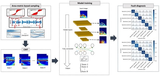
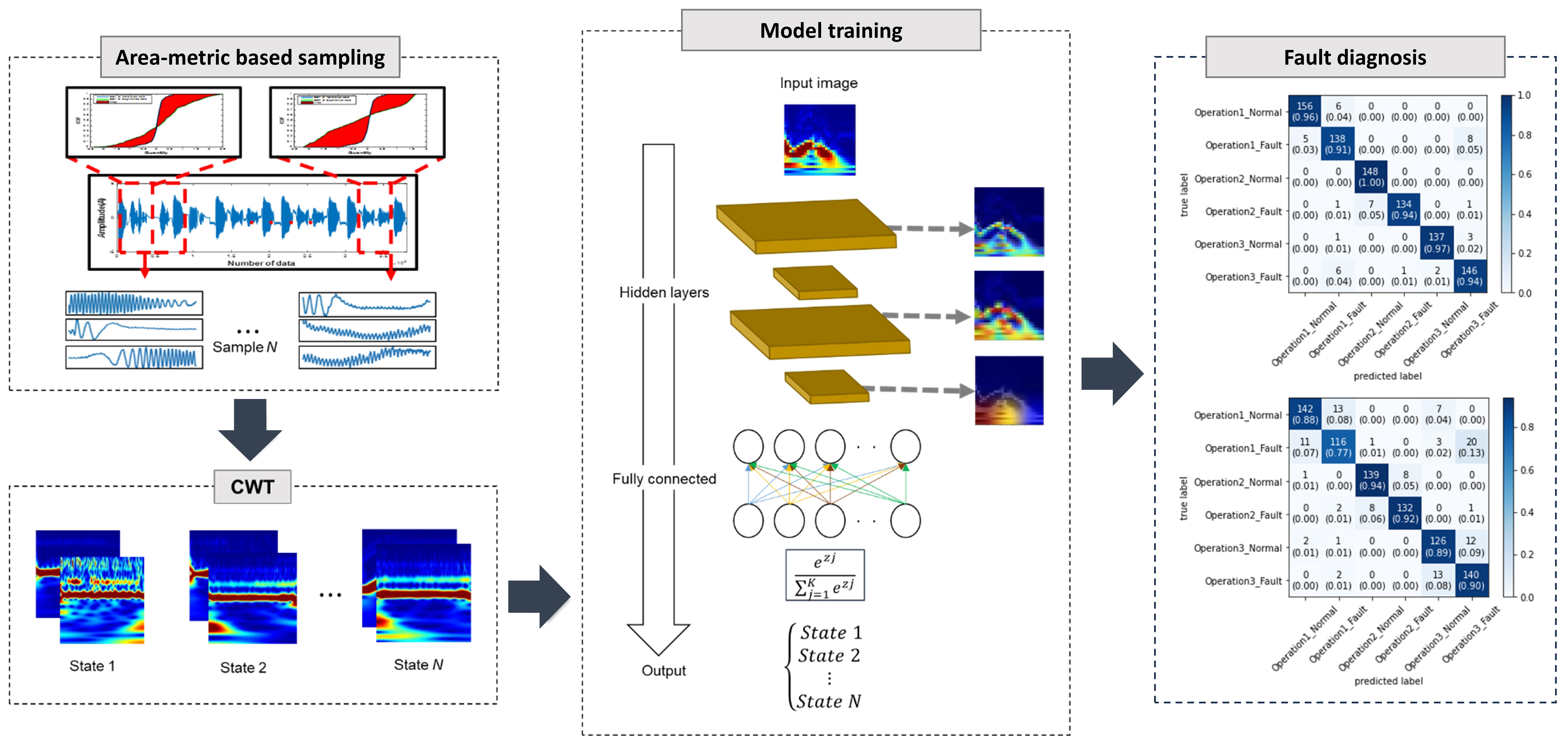
3. Proposed Methodology

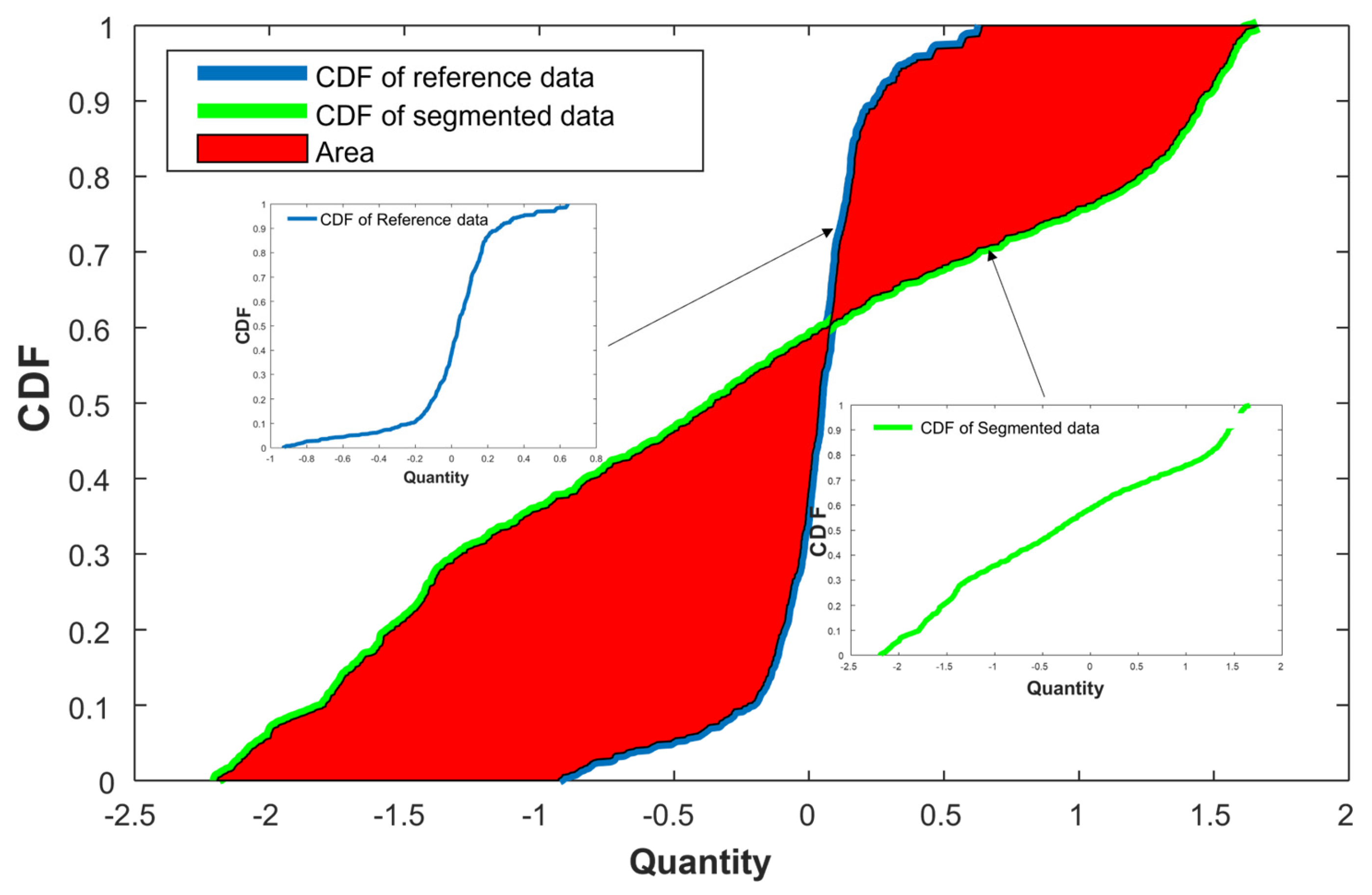
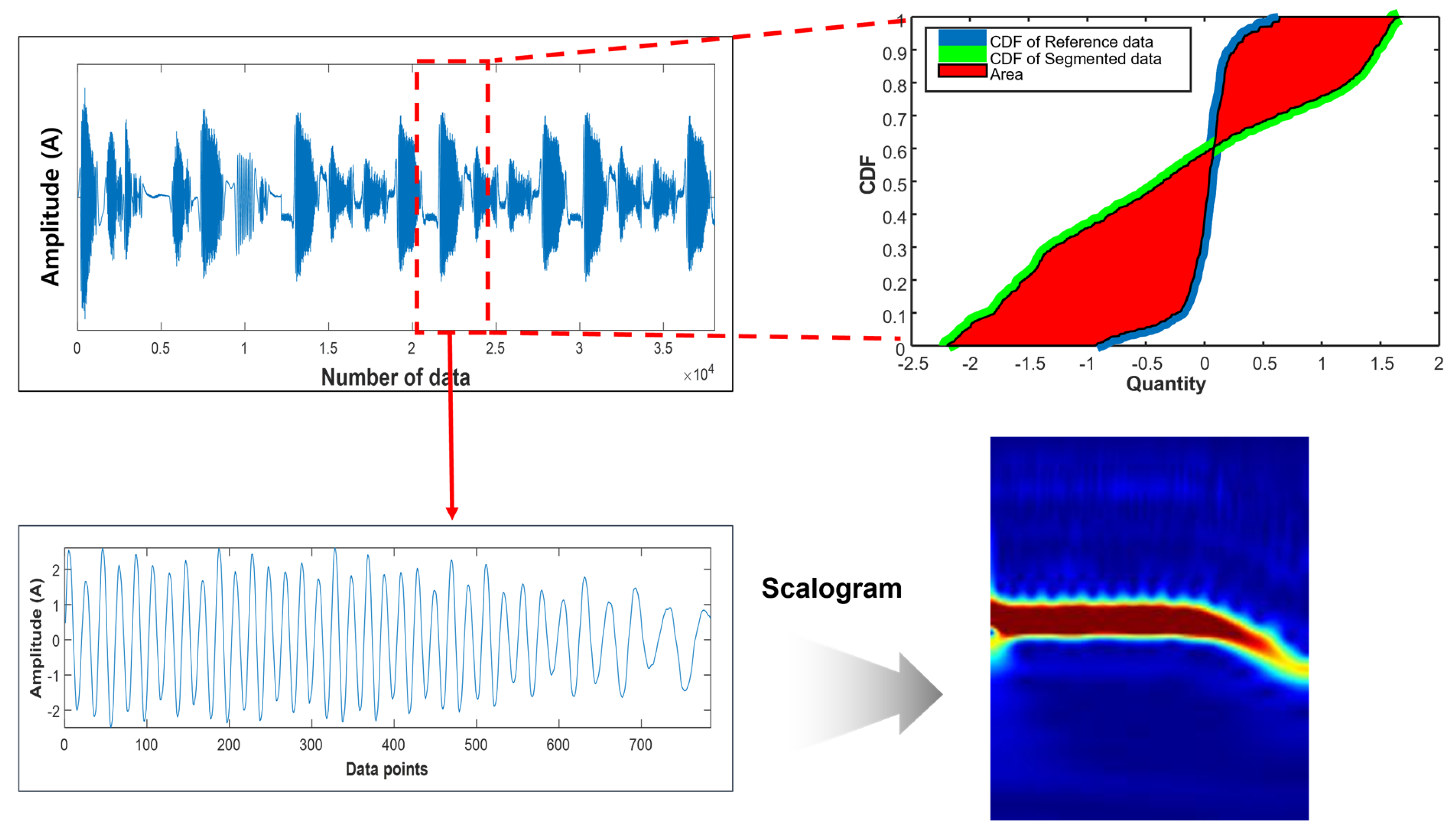
In this section, the theoretical background and explanation of the proposed method are described. Figure 1 shows the flow of the system fault diagnosis method using area-metric-based sampling. First, area-metric-based data sampling identifies locations in datasets that have a potentially high degree of surprise. Second, the sampled data are converted into a continuous wavelet transform (CWT)-based scalogram image containing time–frequency information. Finally, the converted image is trained on an improved CNN model to proceed with classification. The basis for the judgment in each model layer is expressed in a heat map format using XAI.

The choice of the CWT for the data conversion arose from its effectiveness in analyzing signals in both the time and frequency domains simultaneously. Unlike traditional Fourier-based approaches, CWT provides a time-scale representation, making it suitable for the analysis of nonstationary signals. This representation enables the capture of localized features at various scales, a critical aspect for detecting faults in dynamic systems. By utilizing CWT, essential time–frequency characteristics of the signal are preserved, thereby enhancing the representational power for subsequent analysis.

CNNs were employed for fault diagnosis because of their exceptional ability to automatically learn and extract hierarchical features from input data. CNNs excel in pattern recognition tasks, making them apt for our fault diagnosis objectives. The hierarchical feature learning in CNNs, through multiple convolutional layers, enables the model to identify intricate patterns and representations in the transformed data obtained through CWT. CNNs have proven to be highly successful in various signal processing and image recognition tasks, making them a suitable choice for our fault diagnosis application. The integration of CWT for data transformation and CNN for fault diagnosis represents a synergistic approach that leverages the strengths of each method. CWT improves the data representation by extracting meaningful features in the time–frequency domains, and CNN efficiently learns and processes these features to classify and diagnose faults. This combination ensures that the diagnostic model can effectively recognize fault patterns in the transformed data, contributing to accurate and reliable fault diagnosis in nonstationary systems.

3.1. Area Metric

The area metric is a validation metric that performs quantitative comparisons mainly by calculating the area difference between the cumulative distribution function (CDF) graph of simulation prediction, and the CDF of the actual experimental results [36]. As the graph area difference is small, it can be expected that the simulation prediction result is similar to the actual data [36]. The CDF calculation for the comparison target is required to perform the area metric. The CDF of the random variable $\left(X\right)$ is defined as follows:

$$F_X\left(x\right)=P\left(X\le x\right), \mathrm{f}\mathrm{o}\mathrm{r} \mathrm{a}\mathrm{l}\mathrm{l} x\in \mathbb{R}$$

(1)

As shown in Figure 2, the area metric ($M$) is represented as the area between the experimental results CDF ($F_a\left(x\right)$) and the simulation prediction results ($F_s\left(x\right))$ [37].

$$M=\frac{1}{{\overline{\mu }}^a}{\int }_{-\infty }^{\infty }\left|F_s\left(x\right)-F_a\left(x\right)\right|dx$$

(2)

where ${\overline{\mu }}^a$ is the absolute mean of the actual data, and M is normalized by ${\overline{\mu }}^a$. In this study, an area-metric-based approach was employed for data scanning and analysis. The computed area-based metrics provide a quantifiable measure of the dissimilarity between the experimental and simulated CDFs, aiding in assessing the accuracy of the simulation predictions. A smaller area metric indicates a closer match between the experimental and simulated data distributions, signifying a more reliable simulation. Conversely, a larger area metric suggests discrepancies between the experimental and simulated data distributions, indicating areas for potential improvement in the simulation model.

Area-Metric-Based Sampling Method

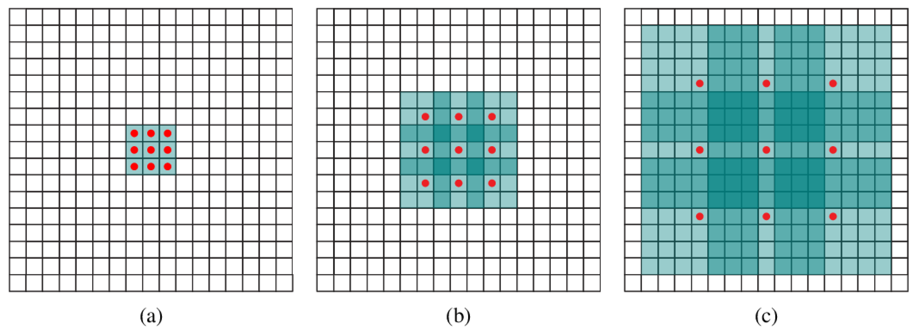
Step 1. Data resampling

Data acquisition (DAQ) collects motor current data for each axis of the robot operating under various operating conditions. Since the data length is different for each operating condition, the data length is set to be the same through resampling. The resampled data ($X_{RE}$), measured through the experiment, is defined as follows:

$$X_{RE}=\{x_{ij}:x_{ij}\in R^{n\times m}\}$$

(3)

The data can be represented by an $n\times m$ matrix ($i=1, 2, \cdots ,n$,$j=1, 2, \cdots ,m$). Each row $x_i\in R^{n\times 1}$ is the resampled data from the DAQ, and each column $x_j\in R^{1\times m}$ is the number of different operating conditions.

Step 2. Data segmentation and area metric calculation

In this study, the empirical cumulative distributive function (ECDF) is derived for the area metric calculation. Based on the resampled data, a reference ECDF, $F_{RE}\left(x\right),$ which can indicate the trend of the entire data, is derived from the entire scenario data for each operating condition. The reference ECDF is defined as follows, where $I$ represents an indicator function:

$$F_{RE}\left(x\right)=\frac{1}{m}\sum _{i=1}^{m}I\left[x_i\le x\right]$$

(4)

As shown in Figure 3a, the data are segmented into a specific window size $(k$) to find the abnormal part of the data. Thus, the segmented data ($X_{SE}$) are defined as:

$$X_{SE}={\{x}_{ij}:x_{ij}\in R^{k\times l}\}, i=1, 2, \cdots , k, j=1, 2, \cdots , l$$

(5)

Figure 3b shows the representation of the reference ECDF and the segmented data ECDF, offering a graphical understanding of the comparison crucial for the subsequent analysis and decision making.

Where, $X_{SE}$ is represented by a $k\times l$ matrix. Each row, $x_i\in R^{k\times 1}$, denotes each segmented data divided into $k$ lengths, while each column, $x_j\in R^{1\times l}$, denotes the number of segmented data.

Each segmented data are converted into an ECDF. The ECDF of the segmented data, $F_{SE}\left(x\right),$ is defined as:

$$F_{SE}\left(x\right)=\frac{1}{l}\sum _{k=1}^{l}I\left[x_k\le x\right]$$

(6)

The area metrics ($M_{RE-SE}$) can be determined by calculating the area difference between the ECDFs of the reference and the segmentation data:

$$M_{RE-SE}=\frac{1}{{\overline{\mu }}^{SE}}{\int }_{-\mathrm{\infty }}^{\mathrm{\infty }}\left|F_{RE}\left(x\right)-F_{SE}\left(x\right)\right|\mathrm{d}\mathrm{x}$$

(7)

Step 3. Data sampling

The data are sequentially scanned for each operating condition, and the area metrics of the reference ECDF and the segmented data ECDF are obtained. The difference in the area metrics between the reference ECDF and the segmented data ECDF is calculated to identify the segments of data that significantly deviate from the overall data trend. Figure 4 illustrates a schematic of the area-metric-based sampling.

Step 4. Time–frequency imaging

Unlike other time–frequency analysis methods, a wavelet transform provides multiresolution to facilitate dynamic analysis in the time–frequency domain. The wavelet transform is a method of decomposing a signal into different frequency bands through a wavelet function in the form of a wave [38]. The wavelet transform is performed using the dot product of the original signal and a set of wavelets. The set of wavelets, called analyzing wavelet or continuous wavelet, is a wavelet family realized through translating and scaling the basic wavelet, $\psi \left(t\right)$. The continuous wavelet can be described as:

$${\psi }_{a,b}(t)={\left|a\right|}^{-1/2} \psi (\frac{t-b}{a})$$

(8)

where $a$ is the scale parameter, and $b$ is the orientation parameter.

The wavelet transform has high-frequency and low-time resolution in the low-frequency band [39]. Still, it has high-time resolution and low-frequency resolution in the high-frequency band [39]. The CWT of the signal $x\left(t\right)$ can be conducted through a convolution operation between $x\left(t\right)$ and the complex conjugate of the wavelet family. If $a$ is continuous variables, the CWT of the signal with finite energy ($Wx\left(a,b\right)$) is mathematically defined as [40]:

$$Wx\left(a,b\right)=〈x\left(t\right),{\psi }_{a,b}(t)〉={\left|a\right|}^{-1/2}{\int }_{-\infty }^{\infty }{x\left(t\right) \psi }^{*}\left(\frac{t-b}{a}\right)dt$$

(9)

where ${ \psi }^{*}$ is the complex conjugate of $\psi$. The absolute value of the CWT of a signal is the scalogram. The CWT of the signal can be represented as an image via a scalogram. The energy of $x\left(t\right)$ at scale $a$ $\left(S\left(a\right)\right)$ is as follows:

$$S\left(a\right)=‖Wx\left(a,b\right)‖={\left({\int }_{-\infty }^{\infty }{\left|Wx\left(a,b\right)\right|}^{2}db\right)}^{\frac{1}{2}}$$

(10)

Figure 5 shows the conversion of a sample extracted by area metric data sampling to a CWT-scalogram:

3.2. Dilated CNN

To solve complex problems and improve accuracy, the CNN structure is deepened by stacking layers, and the number of hyperparameters and parameters increases accordingly. Sometimes, this feature causes fatal drawbacks. As the network layer increases, backpropagation of the gradient suffers from vanishing gradient problems [41]. This may result in a sharp drop or saturation in the network performance. The issues mentioned above can be mitigated through dilated CNN. As shown in Figure 6, the dilated CNN is performed using dilated convolution kernels, unlike the traditional CNN, which uses traditional convolutional kernels.

Let $P_0, P_1, \cdots , P_{n-1}: {\mathbb{Z}}^2\to \mathbb{R}$ be discrete functions, and ${\omega }_0, {\omega }_1, \cdots , {\omega }_{n-2}: \mathsf{\Omega }\to \mathbb{R}$ be discrete filter with size $3\times 3$. For the application of filters with exponentially increasing dilation, this can be expressed as:

$$P_{k+1}=P_k\mathrm{\ast }{}_{2^k} {\omega }_0 for k=1,2,\cdots ,n-2$$

(11)

The receptive field of an element $\mathsf{\beta }$, a component of $P_{k+1}$, is defined as a set of elements existing in $P_0$ that can estimate the value of $P_{k+1}$($\mathsf{\beta }$). The size of the receptive field of each component in $P_{k+1}$ is ${(2}^{k+2}-1\left)\right(2^{k+2}-1)$. Figure 7 shows the convolutional kernel according to the dilation rate. In Figure 7a, $P_1$ is made from $P_0$ by a one-dilated convolution in which every element in $P_1$ has a receptive field of size 3 × 3. (Figure 7b) $P_2$ is made from $P_1$ by a two-dilated convolution, in which every element in $P_2$ has a receptive field of size 7 × 7. (Figure 7c) $P_3$ is made from $P_2$ by a two-dilated convolution in which every element in $P_2$ has a receptive field of size 15 × 15. As the dilation rate increases, the receptive field becomes more expansive, but the number of parameters remains the same. More information can be accommodated through this dilated convolution kernel without increasing the amount of computation.

3.3. Grad-CAM

CAM is applicable only to CNN models based on global average pooling (GAP) architecture, but Grad-CAM is a model that can be applied to CNN models of other structures. Grad-CAM obtains a class activation map by calculating the gradient of the class score ($y^c$), for class, with respect to feature maps ($A^k$) of the convolutional layer. Then, a global average pooling on the gradient flowing back can be performed:

$$a_k^c=\frac{1}{Z} \sum _i\sum _j\frac{\partial y^c}{\partial A_{ij}^k}$$

(12)

where $i, j$ represent each pixel of the feature map, $A^k$. $H$ and $W$ are rows and columns, and $Z$ represents the number of pixels of the $A^k$. Weight $a_k^c$ captures the importance of feature map $A^k$. Based on Equation (13), the rectified linear unit (ReLU) can be derived by removing negative values [43]:

$$L_{Grad-CAM}^c=ReLU \left(\sum _k{a}_k^c{A}^k\right)$$

(13)

4. Case Study

4.1. Data Acquisition System

This study introduces the methodologies introduced in Section 3 for robotic strain wave gear reducer fault diagnosis (the Robostar R004 welding robot with 6 degrees of freedom). Each axis of the robot is controlled by repeating acceleration/deceleration through a servomotor. As shown in Figure 8, the robotic strain wave gear reducer has two states: normal and faulty. The fault type is the bearing inner ring defect, and the failure is applied to axis 3.

Table 3. Description of the robot.

Parameter	Properties
Robot type	Robostar R004 welding robot
Sensitivity of sensor	64 mV/A
Health state	Normal, fault
Fault type	Strain Wave gear fault (bearing inner ring fault) in axis 3
Data type	1st phase of electrical current
Sampling frequency	2048 Hz

shows detailed information on the robot:

4.2. Experimental Set-Up

In this study, we analyze normal and fault motor current data in the 3rd axis to which faults are applied. The experiment was performed, as shown in Figure 9. The current data collection system is as follows. The robot operation cycle was divided using the programmable logic controller (PLC). The PLC provides trigger signals at the start and end of the robot motion, and stores them in the PC. All axes of the robot are equipped with WCS2720 sensors, which are based on the Hall effect. The sensor signals are collected through the DAQ module, and the sampling rate was fs = 2048 Hz.

Target robots are widely used for body welding.

Table 4. Operating condition specifications.

Motion	Properties	Data Size
Operation 1 (A → B)	1. A-point welding 2. Moving from A to B (40% of the maximum operating speed)	(27, 839, 10)
Operation 2 (B → C)	1. B-point welding 2. Moving from B to C (20% of the maximum operating speed)	(37, 799, 10)
Operation 3 (C → D)	1. C-point welding 2. Moving from C to D (60% of the maximum operating speed)	(25, 634, 10)

shows detailed information on the robot’s operating conditions. A total of six working conditions (Operation 1_Normal, Operation 1_Fault, Operation 2_Normal, Operation 2_Fault, Operation 3_Normal, and Operation 3_Fault) used for car body welding were set. The robot operates under the set operating conditions. The robot repeats the welding motion in the sequence of car door points A–B–C–D, as shown in Figure 9c. After welding each point (A, B, C, and D), the robot moves to the next point (e.g., A → B, B → C, C → D). First, the robot completes the A-point welding of the car door in Operation 1. After that, it moves to point B at 40% of the maximum operating speed. In Operation 2, after the welding is completed at point B, it moves to point C at a rate of 20% of the maximum operating speed. In Operation 3, when it is completed at point C, it moves to point D at the maximum operating speed of 60%, and completes welding at point D. Figure 10 shows the motor current signal according to the robot’s operating conditions.

In this study, 500 samples of length (28 × 28) were extracted using the previously proposed area metric sampling method under each of six operating and health conditions, as summarized in

Table 5. Description of the health condition in the experimental dataset.

Type	Number of Samples
Operation 1_Normal	500
Operation 1_Fault	500
Operation 2_Normal	500
Operation 2_Fault	500
Operation 3_Normal	500
Operation 3_Fault	500

. Afterward, the extracted samples were converted into CWT-based scalogram images, and classified through a deep learning model.

Table 6. Examples of the converted CWT-scalogram images in the experimental dataset.

Type	Normal	Fault
Operation 1
Operation 2
Operation 3

shows examples sampled of converted CWT-scalogram images in the experimental dataset using the proposed method.

5. Results and Discussion

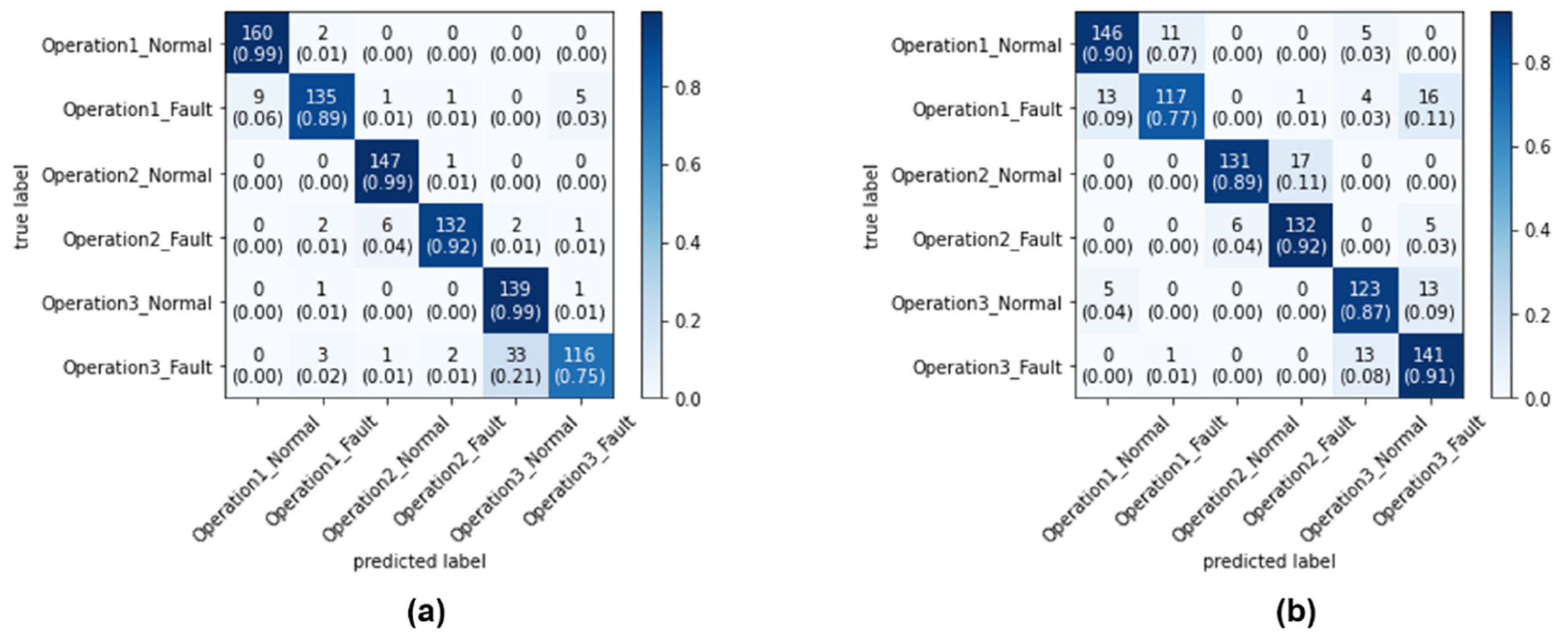
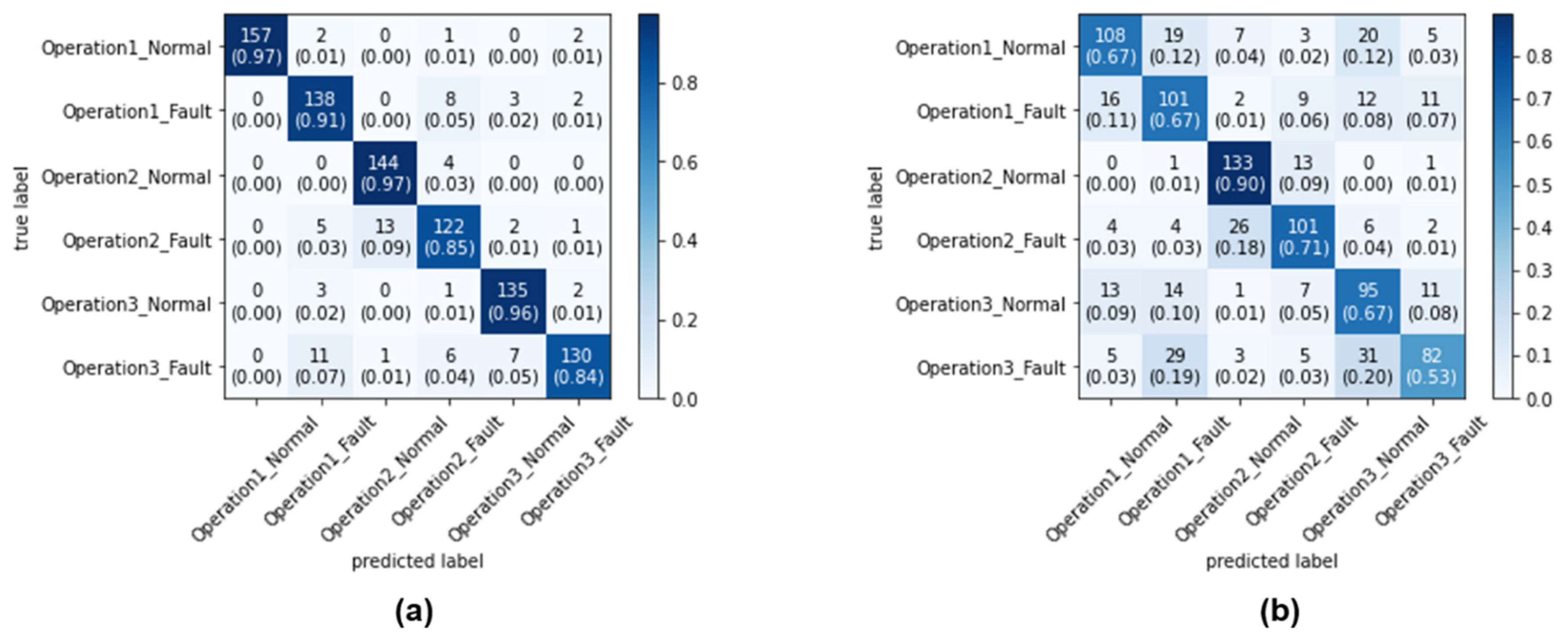
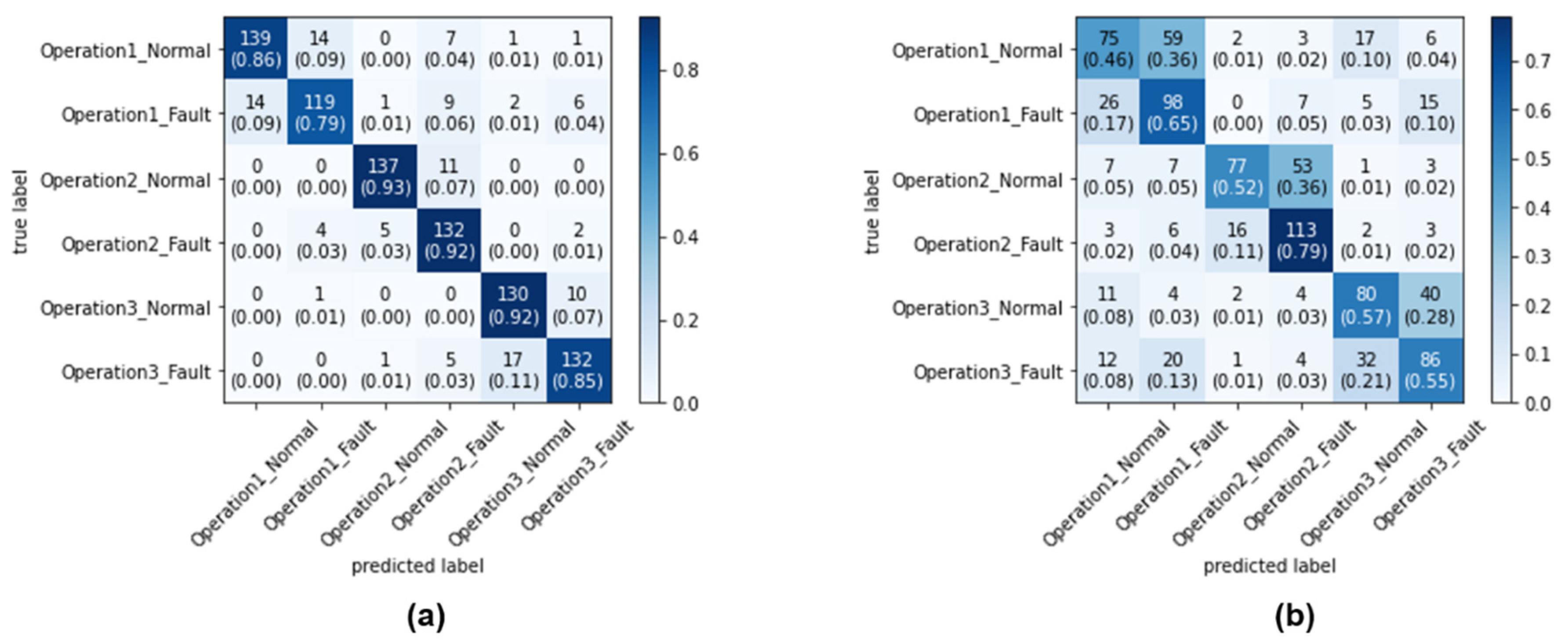
5.1. Evaluation of the Proposed Method

The proposed methodology is verified by comparison with previous studies.

Table 7. Description of the comparison target.

Methods	Input Data
Area-metric-based sampling	CWT-scalogram (proposed method)
	STFT-spectrogram
	Grayscale image
	1D raw signal
Random sampling	CWT-scalogram
	STFT-spectrogram
	Grayscale image
	1D raw signal

is a previous study to be compared and includes raw signal input, grayscale image input, and STFT-spectrogram input.

The performance of the proposed method was evaluated using accuracy among the four evaluation indicators (precision, recall, F1-score, and accuracy) shown in

Table 8. Evaluation indicators.

Metric	Equation
Precision	$\frac{TP}{TP+FP}$
Recall	$\frac{TP}{TP+FN}$
F1-score	$\frac{2\ast Precision\ast Recall}{Precision+Recall}$
Accuracy	$\frac{TP+TN}{TP+TN+FP+FN}$

. Precision is the proportion of actual true data among the data judged to be true by the model. Conversely, recall is the proportion of data judged to be true by the model out of the actual true data. The F1-score is the harmonic mean value of the precision and recall. Accuracy is the proportion of data that the model correctly predicted out of the total data.

In Table 8, $TP$ denotes the true positive, $FP$ is the false positive, $TN$ represents the true negative, and $FN$ represents the false negative. Dilated CNN and traditional CNN models have an adaptive moment algorithm optimizer with a batch size of 32 set as the optimization algorithm for fast convergence. The execution rate was set to 0.001. For both models, a total of 100 training epochs were performed. Of the total data, the training data and test data were divided into 70 and 30%. Figure 11 shows a structural diagram of the CNN model. The proposed dilated CNN and the traditional CNN model had the same structure, but, in the case of the proposed dilated CNN model, a dilation rate = 2 was applied in the convolutional layer.

Table 9. The results of the various methods.

Method	Area-Metric-Based Sampling				Random Sampling
	Precision (%)	Recall (%)	F1-Score (%)	Accuracy (%)	Precision (%)	Recall (%)	F1-Score (%)	Accuracy (%)
Dilated-CNN using CWT-scalogram	95.57	95.46	95.49	95.44	88.55	88.40	88.36	88.33
CNN using CWT-scalogram	92.53	92.20	91.98	92.11	88.12	87.77	87.77	87.78
CNN using STFT-spectrogram	91.76	91.76	91.66	91.78	69.29	69.05	68.70	68.89
CNN using Grayscale image	87.80	87.81	87.68	87.67	60.18	59.08	58.77	58.78
CNN using 1D raw signal	83.33	83.52	83.25	83.44	49.82	50.06	49.72	48.89

summarizes the performance comparisons of the various methods. In the traditional CNN model, the raw signal input shows a classification accuracy of 48.89% when sampled with random sampling and 83.44% with area-metric-based sampling. The grayscale image input shows a classification accuracy of 58.78% when sampled with random sampling and 87.67% with area-metric-based sampling. The STFT-spectrogram input shows a classification accuracy of 68.89% when sampling with random sampling and 91.78% classification accuracy when sampling with area-metric-based sampling. The CWT-scalogram input shows an accuracy of 87.78% when sampling with random sampling. When sampling with area-metric-based sampling, the classification accuracy is 92.11%. When training with dilated-CNN, the classification accuracy for CWT-scalogram input is 88.33% for random sampling and 95.44% for area-metric sampling, confirming that the classification accuracy improved to 0.55 and 3.33%, respectively. The proposed method shows the highest accuracy among the comparison group. This means that the classification performance is the best.

Figure 12 shows the confusion matrix of the dilated-CNN using the CWT-scalogram results for area-metric-based sampling and random sampling. Figure 13 shows the confusion matrix of the CNN using the CWT-scalogram results for the area-metric-based sampling and random sampling. Figure 14 shows the confusion matrix of the CNN using the STFT-spectrogram results for the area-metric-based sampling and random sampling. Figure 15 shows the confusion matrix of the CNN using the grayscale image results for area-metric-based sampling and random sampling. Figure 16 shows the confusion matrix of the CNN using 1D raw signal results for area-metric-based sampling and random sampling.

5.2. Presenting the Basis for Judgment: Based on Explainable Artificial Intelligence

Table 10. Attention map of the proposed method for each condition.

	Input	Attention Map
Operation 1 Normal
Operation 1 Fault
Operation 2 Normal
Operation 2 Fault
Operation 3 Normal
Operation 3 Fault

shows the results of the attention map for each state of the proposed method as a heat map based on Grad-CAM. Since the robot is controlled by repeating acceleration and deceleration instantaneously, the frequency changes over time. A CWT-based scalogram representing the change in frequency over time of nonstationary data is used for model training. The model is trained by weighting the time-varying frequency components that have physical meaning in the input image and deriving a result.

Compared to the traditional CNN model, the dilated-CNN derives a classification accuracy improvement of up to 3.33%. Using Grad-CAM, the basis for judgment in each layer is visualized through a heat map to present the basis for improving the classification accuracy. The receptive field becomes more expansive in the convolutional layer of the dilated CNN because dilated convolution kernels are used. In the heat map using Grad-CAM, it can be observed that the dilated-CNN model had more active parts than the traditional CNN model in each convolutional layer. In addition, in a grayscale image in which signals are arranged, a judgment is performed on each layer without any special criteria. On the other hand, in the STFT-spectrogram and CWT-scalogram, which are time–frequency images, each layer performs a judgment by focusing on the frequency component of the image.

Unlike a STFT-spectrogram, a CWT-scalogram provides multiresolution for the time–frequency domains. Since the CWT-scalogram contains various time–frequency information compared to the STFT-spectrogram, it provides improved classification accuracy, because there are many areas where judgment weights are placed in each layer.

Table 11. The basis for judgment in each layer visualized through a heat map.

	Input	Convolution Layer 1	Convolution Layer 2	Convolution Layer 3
Dilated-CNN using CWT-scalogram
CNN using CWT-scalogram
CNN using STFT-spectrogram
CNN using Grayscale image

is the result of visualizing the weights in each convolutional layer as a heat map using the Grad-CAM.

6. Conclusions

In this research, a new data sampling method was developed to solve the problems of data imbalance and shortage. In addition, we introduced the judgment basis for deep learning-based defect diagnosis using XAI. The proposed method was verified using data of nonstationary current signals from industrial robots operating under various operating conditions. The verification results are summarized as follow.

First, the data were extracted using area-metric-based sampling. The data were scanned sequentially for each operating condition, and the area metrics of the reference ECDF and segmented data ECDF were obtained. Second, The sampled data were transformed into CWT–scalogram images containing time–frequency information. A dilated CNN using dilated convolution kernels was introduced to increase the receptive field, which made it possible to accommodate a lot of information without increasing the number of computations and number of hyperparameters. Third, the proposed method was verified by performing robotic strain wave gear reducer fault diagnosis. The test classification accuracy, precision, recall, and F1-score were used as evaluation indices. As a result, the proposed method showed the highest accuracy among the comparison groups at 95.44%, which means that the classification performance is the best. For all comparison groups, area-metric-based sampling showed a higher test classification accuracy by at least 4.33% and up to 34.55% than the conventional random sampling. This indicates that the proposed area-based sampling can overcome the limitations of traditional sampling, and solve the problem of data imbalance and shortage. In addition, the CWT–scalogram showed a minimum of 0.33% and a maximum of 38.89% higher test classification accuracy compared to other input data under the same comparison criteria. This indicates that the CWT-scalogram has the least data loss compared to other data analysis methods. When a dilated CNN was used instead of the traditional CNN as a classification model, the test classification accuracy improved by at least 0.55% and, at most, 3.33%. Through Grad-CAM, the basis for judgment in the convolutional layer of the two models was presented using a heat map. Compared to the traditional CNN, the dilated CNN had more active parts, indicating that the dilated CNN was based on more feature information than the traditional CNN. The proposed method can derive high diagnostic accuracy even with a small amount of data, so it can be applied to industries where it is difficult to secure sufficient quality data. In addition, by presenting the basis for the diagnosis result, the reliability of the diagnosis model can be increased, and it can be widely applied to actual industrial sites. Future work will involve further exploring the adaptability and robustness of the proposed method across different industrial domains and expanding the dataset to encompass a broader range of operating conditions for a comprehensive validation of the approach. Additionally, investigating ensemble techniques and exploring real-time implementation possibilities will be essential steps to enhance the method’s practical applicability.

References

1. Jing, L.; Zhao, M.; Li, P.; Xu, X. A Convolutional Neural Network Based Feature Learning and Fault Diagnosis Method for the Condition Monitoring of Gearbox. Measurement 2017, 111, 1–10. [Google Scholar] [CrossRef]
2. Zhou, W.; Lu, B.; Habetler, T.G.; Harley, R.G. Incipient Bearing Fault Detection via Motor Stator Current Noise Cancellation Using Wiener Filter. IEEE Trans. Ind. Appl. 2009, 45, 1309–1317. [Google Scholar] [CrossRef]
3. Huang, K.; Wu, S.; Li, Y.; Yang, C.; Gui, W. A Multi-Rate Sampling Data Fusion Method for Fault Diagnosis and Its Industrial Applications. J. Process Control 2021, 104, 54–61. [Google Scholar] [CrossRef]
4. Kankar, P.K.; Sharma, S.C.; Harsha, S.P. Fault Diagnosis of Ball Bearings Using Machine Learning Methods. Expert Syst. Appl. 2011, 38, 1876–1886. [Google Scholar] [CrossRef]
5. Samanta, S.; Bera, J.N.; Sarkar, G. KNN Based Fault Diagnosis System for Induction Motor. In Proceedings of the 2016 2nd International Conference on Control, Instrumentation, Energy & Communication (CIEC), Kolkata, India, 28–30 January 2016; pp. 304–308. [Google Scholar]
6. Widodo, A.; Kim, E.Y.; Son, J.-D.; Yang, B.-S.; Tan, A.C.C.; Gu, D.-S.; Choi, B.-K.; Mathew, J. Fault Diagnosis of Low Speed Bearing Based on Relevance Vector Machine and Support Vector Machine. Expert Syst. Appl. 2009, 36, 7252–7261. [Google Scholar] [CrossRef]
7. Zhang, S.; Zhang, S.; Wang, B.; Habetler, T.G. Deep Learning Algorithms for Bearing Fault Diagnostics—A Comprehensive Review. IEEE Access 2020, 8, 29857–29881. [Google Scholar] [CrossRef]
8. Khan, A.; Hwang, H.; Kim, H.S. Synthetic Data Augmentation and Deep Learning for the Fault Diagnosis of Rotating Machines. Mathematics 2021, 9, 2336. [Google Scholar] [CrossRef]
9. Mikołajczyk, A.; Grochowski, M. Data Augmentation for Improving Deep Learning in Image Classification Problem. In Proceedings of the 2018 International Interdisciplinary PhD Workshop (IIPhDW), Świnouście, Poland, 9–12 May 2018; pp. 117–122. [Google Scholar]
10. Wang, J.; Mall, S.; Perez, L. The Effectiveness of Data Augmentation in Image Classification Using Deep Learning. arXiv 2017, arXiv:1712.04621. [Google Scholar]
11. Guennec, A.L.; Malinowski, S.; Tavenard, R. Data Augmentation for Time Series Classification Using Convolutional Neural Networks. In ECML/PKDD Workshop on Advanced Analytics and Learning on Temporal Data; Springer: Berlin/Heidelberg, Germany, 2016. [Google Scholar]
12. Um, T.T.; Pfister, F.M.J.; Pichler, D.; Endo, S.; Lang, M.; Hirche, S.; Fietzek, U.; Kulić, D. Data Augmentation of Wearable Sensor Data for Parkinson’s Disease Monitoring Using Convolutional Neural Networks. In Proceedings of the 19th ACM International Conference on Multimodal Interaction, Glasgow, UK, 13–17 November 2017; Association for Computing Machinery: New York, NY, USA, 2017; pp. 216–220. [Google Scholar]
13. Li, Y.; Hu, H.; Zhou, G. Using Data Augmentation in Continuous Authentication on Smartphones. IEEE Internet Things J. 2019, 6, 628–640. [Google Scholar] [CrossRef]
14. Frid-Adar, M.; Klang, E.; Amitai, M.; Goldberger, J.; Greenspan, H. Synthetic Data Augmentation Using GAN for Improved Liver Lesion Classification. In Proceedings of the 2018 IEEE 15th International Symposium on Biomedical Imaging (ISBI 2018), Washington, DC, USA, 4–7 April 2018; pp. 289–293. [Google Scholar]
15. Chen, H.-Y.; Lee, C.-H. Vibration Signals Analysis by Explainable Artificial Intelligence (XAI) Approach: Application on Bearing Faults Diagnosis. IEEE Access 2020, 8, 134246–134256. Available online: https://ieeexplore.ieee.org/abstract/document/9131692 (accessed on 2 November 2022). [CrossRef]
16. Xie, T.; Huang, X.; Choi, S.-K. Intelligent Mechanical Fault Diagnosis Using Multisensor Fusion and Convolution Neural Network. IEEE Trans. Ind. Inform. 2022, 18, 3213–3223. [Google Scholar] [CrossRef]
17. Hoang, D.T.; Kang, H.J. A Motor Current Signal-Based Bearing Fault Diagnosis Using Deep Learning and Information Fusion. IEEE Trans. Instrum. Meas. 2020, 69, 3325–3333. [Google Scholar] [CrossRef]
18. Janssens, O.; Slavkovikj, V.; Vervisch, B.; Stockman, K.; Loccufier, M.; Verstockt, S.; Van de Walle, R.; Van Hoecke, S. Convolutional Neural Network Based Fault Detection for Rotating Machinery. J. Sound Vib. 2016, 377, 331–345. [Google Scholar] [CrossRef]
19. Park, S.; Song, J.; Kim, H.S.; Ryu, D. Non-Contact Detection of Delamination in Composite Laminates Coated with a Mechanoluminescent Sensor Using Convolutional AutoEncoder. Mathematics 2022, 10, 4254. [Google Scholar] [CrossRef]
20. Saufi, S.R.; Ahmad, Z.A.B.; Leong, M.S.; Lim, M.H. Gearbox Fault Diagnosis Using a Deep Learning Model with Limited Data Sample. IEEE Trans. Ind. Inform. 2020, 16, 6263–6271. [Google Scholar] [CrossRef]
21. Zhong, C.; Yan, K.; Dai, Y.; Jin, N.; Lou, B. Energy Efficiency Solutions for Buildings: Automated Fault Diagnosis of Air Handling Units Using Generative Adversarial Networks. Energies 2019, 12, 527. [Google Scholar] [CrossRef]
22. Kumar, P.; Hati, A.S. Dilated Convolutional Neural Network Based Model for Bearing Faults and Broken Rotor Bar Detection in Squirrel Cage Induction Motors. Expert Syst. Appl. 2022, 191, 116290. [Google Scholar] [CrossRef]
23. Yang, D.; Liu, Y.; Li, S.; Li, X.; Ma, L. Gear Fault Diagnosis Based on Support Vector Machine Optimized by Artificial Bee Colony Algorithm. Mech. Mach. Theory 2015, 90, 219–229. [Google Scholar] [CrossRef]
24. Qian, L.; Pan, Q.; Lv, Y.; Zhao, X. Fault Detection of Bearing by Resnet Classifier with Model-Based Data Augmentation. Machines 2022, 10, 521. [Google Scholar] [CrossRef]
25. Hu, T.; Tang, T.; Lin, R.; Chen, M.; Han, S.; Wu, J. A Simple Data Augmentation Algorithm and a Self-Adaptive Convolutional Architecture for Few-Shot Fault Diagnosis under Different Working Conditions. Measurement 2020, 156, 107539. [Google Scholar] [CrossRef]
26. Liu, J.; Qu, F.; Hong, X.; Zhang, H. A Small-Sample Wind Turbine Fault Detection Method with Synthetic Fault Data Using Generative Adversarial Nets. IEEE Trans. Ind. Inform. 2019, 15, 3877–3888. [Google Scholar] [CrossRef]
27. Liu, Y.; Jiang, H.; Liu, C.; Yang, W.; Sun, W. Data-Augmented Wavelet Capsule Generative Adversarial Network for Rolling Bearing Fault Diagnosis. Knowl. Based Syst. 2022, 252, 109439. [Google Scholar] [CrossRef]
28. Li, Z.; Zheng, T.; Wang, Y.; Cao, Z.; Guo, Z.; Fu, H. A Novel Method for Imbalanced Fault Diagnosis of Rotating Machinery Based on Generative Adversarial Networks. IEEE Trans. Instrum. Meas. 2021, 70, 3500417. [Google Scholar] [CrossRef]
29. Wang, Y.; Sun, G.; Jin, Q. Imbalanced Sample Fault Diagnosis of Rotating Machinery Using Conditional Variational Auto-Encoder Generative Adversarial Network. Appl. Soft Comput. 2020, 92, 106333. [Google Scholar] [CrossRef]
30. Sairam, S.; Seshadhri, S.; Marafioti, G.; Srinivasan, S.; Mathisen, G.; Bekiroglu, K. Edge-Based Explainable Fault Detection Systems for Photovoltaic Panels on Edge Nodes. Renew. Energy 2022, 185, 1425–1440. [Google Scholar] [CrossRef]
31. Srinivasan, S.; Arjunan, P.; Jin, B.; Sangiovanni-Vincentelli, A.L.; Sultan, Z.; Poolla, K. Explainable AI for Chiller Fault-Detection Systems: Gaining Human Trust. Computer 2021, 54, 60–68. [Google Scholar] [CrossRef]
32. Morichetta, A.; Casas, P.; Mellia, M. EXPLAIN-IT: Towards Explainable AI for Unsupervised Network Traffic Analysis. In Proceedings of the 3rd ACM CoNEXT Workshop on Big DAta, Machine Learning and Artificial Intelligence for Data Communication Networks, Orlando, FL, USA, 9 December 2019; Association for Computing Machinery: New York, NY, USA, 2019; pp. 22–28. [Google Scholar]
33. Shrikumar, A.; Greenside, P.; Kundaje, A. Learning Important Features Through Propagating Activation Differences. In Proceedings of the 34th International Conference on Machine Learning, Sydney, Australia, 6–11 August 2017. [Google Scholar]
34. Selvaraju, R.R.; Cogswell, M.; Das, A.; Vedantam, R.; Parikh, D.; Batra, D. Grad-CAM: Visual Explanations from Deep Networks via Gradient-Based Localization. arXiv 2016, arXiv:1610.02391. [Google Scholar]
35. Hwang, C.; Lee, T. E-SFD: Explainable Sensor Fault Detection in the ICS Anomaly Detection System. IEEE Access 2021, 9, 140470–140486. [Google Scholar] [CrossRef]
36. Hu, J.; Zhou, Q.; McKeand, A.; Xie, T.; Choi, S.-K. A Model Validation Framework Based on Parameter Calibration under Aleatory and Epistemic Uncertainty. Struct. Multidiscip. Optim. 2021, 63, 645–660. [Google Scholar] [CrossRef]
37. Lee, D.; Kim, N.H.; Kim, H.-S. Validation and Updating in a Large Automotive Vibro-Acoustic Model Using a P-Box in the Frequency Domain. Struct. Multidiscip. Optim. 2016, 54, 1485–1508. [Google Scholar] [CrossRef]
38. Strang, G.; Nguyen, T. Wavelets and Filter Banks; SIAM: Bangkok, Thailand, 1996; ISBN 978-0-9614088-7-9. [Google Scholar]
39. Barros, J.; Diego, R.I. Analysis of Harmonics in Power Systems Using the Wavelet Packet Transform. In Proceedings of the 2005 IEEE Instrumentationand Measurement Technology Conference Proceedings, Ottawa, ON, Canada, 16–19 May 2005; Volume 2, pp. 1484–1488. [Google Scholar]
40. Liang, P.; Deng, C.; Wu, J.; Yang, Z.; Zhu, J.; Zhang, Z. Single and Simultaneous Fault Diagnosis of Gearbox via a Semi-Supervised and High-Accuracy Adversarial Learning Framework. Knowl. Based Syst. 2020, 198, 105895. [Google Scholar] [CrossRef]
41. Li, Y.; Zhang, X.; Chen, D. CSRNet: Dilated Convolutional Neural Networks for Understanding the Highly Congested Scenes. In Proceedings of the IEEE Conference on Computer Vision and Pattern Recognition (CVPR), Salt Lake City, UT, USA, 19–21 June 2018; pp. 1091–1100. [Google Scholar]
42. Yu, F.; Koltun, V. Multi-Scale Context Aggregation by Dilated Convolutions. arXiv 2016, arXiv:1511.07122. [Google Scholar]
43. Gozzi, N.; Malandri, L.; Mercorio, F.; Pedrocchi, A. XAI for Myo-Controlled Prosthesis: Explaining EMG Data for Hand Gesture Classification. Knowl. Based Syst. 2022, 240, 108053. [Google Scholar] [CrossRef]
Figure 1. Overall process of the proposed fault diagnosis method.
Mathematics 11 04081 g001
Figure 2. Illustration depicting the computation of the area-based metrics.
Mathematics 11 04081 g002
Figure 3. (a) Segmentation of data into specific window sizes ( k ) to identify anomalous segments within the dataset. (b) Representation of the reference CDF and the segmented data CDF.
Mathematics 11 04081 g003
Figure 4. The area-metric-based sampling method.
Mathematics 11 04081 g004
Figure 5. Time–frequency imaging based on CWT.
Mathematics 11 04081 g005
Figure 6. Deep learning model framework: (a) CNN model; (b) dilated-CNN.
Mathematics 11 04081 g006
Figure 7. (a) Receptive field change according to the dilation rate (b) Two-dilated convolution with a receptive field of size 7 × 7 (c) Two-dilated convolution with a receptive field of size 15 × 15 [42].
Mathematics 11 04081 g007
Figure 8. Target robot Robostar R004 and fault types.
Mathematics 11 04081 g008
Figure 9. Experimental set-up of target robot: (a) experimental set-up; (b) car body welding; (c) welding points of car door.
Mathematics 11 04081 g009
Figure 10. Various operation conditions: (a) normal and fault states of Operation 1; (b) normal and fault state of Operation condition 2; (c) normal and fault states of Operation 3.
Mathematics 11 04081 g010
Figure 11. Structure of the CNN model.
Mathematics 11 04081 g011
Figure 12. Testing confusion matrix of the dilated-CNN using CWT-scalogram: (a) area-metric-based sampling method confusion matrix (95.44% accuracy); (b) random sampling method confusion matrix (88.33% accuracy).
Mathematics 11 04081 g012
Figure 13. Testing the confusion matrix of the CNN using CWT-scalogram: (a) area-metric-based sampling method confusion matrix (92.11% accuracy); (b) random sampling method confusion matrix (87.78% accuracy).
Mathematics 11 04081 g013
Figure 14. Testing confusion matrix of the CNN using STFT-spectrogram: (a) area-metric-based sampling method confusion matrix (91.76% accuracy); (b) random sampling method confusion matrix (68.89% accuracy).
Mathematics 11 04081 g014
Figure 15. Testing confusion matrix of the CNN using grayscale image: (a) area-metric-based sampling method confusion matrix (87.67% accuracy); (b) random sampling method confusion matrix (58.78% accuracy).
Mathematics 11 04081 g015
Figure 16. Testing confusion matrix of the CNN using grayscale image: (a) area-metric-based sampling method confusion matrix (83.44% accuracy); (b) random sampling method confusion matrix (48.89% accuracy).
Mathematics 11 04081 g016