Author Contributions
I.A., M.Y. and F.B.M.B.; methodology, M.A. and S.K.; software, M.Y., M.A. and S.K.; validation, I.A., M.Y. and F.B.M.B.; formal analysis, M.Y., M.A. and S.K.; investigation, I.A., M.Y., M.A., S.K. and F.B.M.B.; resources, I.A.; writing—original draft preparation, M.Y., M.A. and S.K.; writing—review and editing, I.A., M.Y., M.A., S.K. and F.B.M.B.; supervision, M.Y.; project administration, I.A., M.Y., M.A., S.K. and F.B.M.B.; funding acquisition, I.A. All authors have read and agreed to the published version of the manuscript.
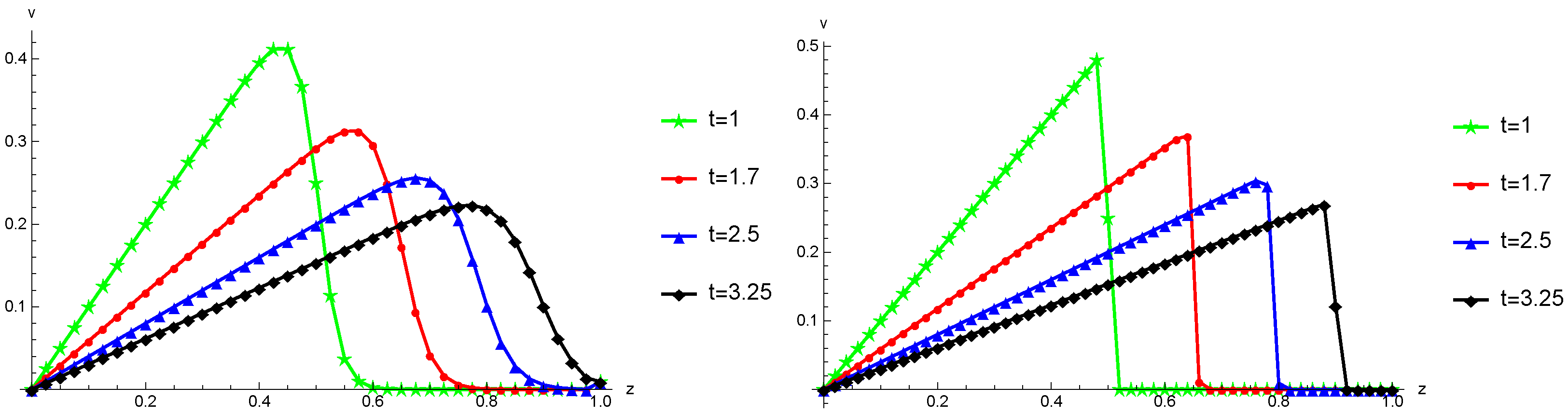
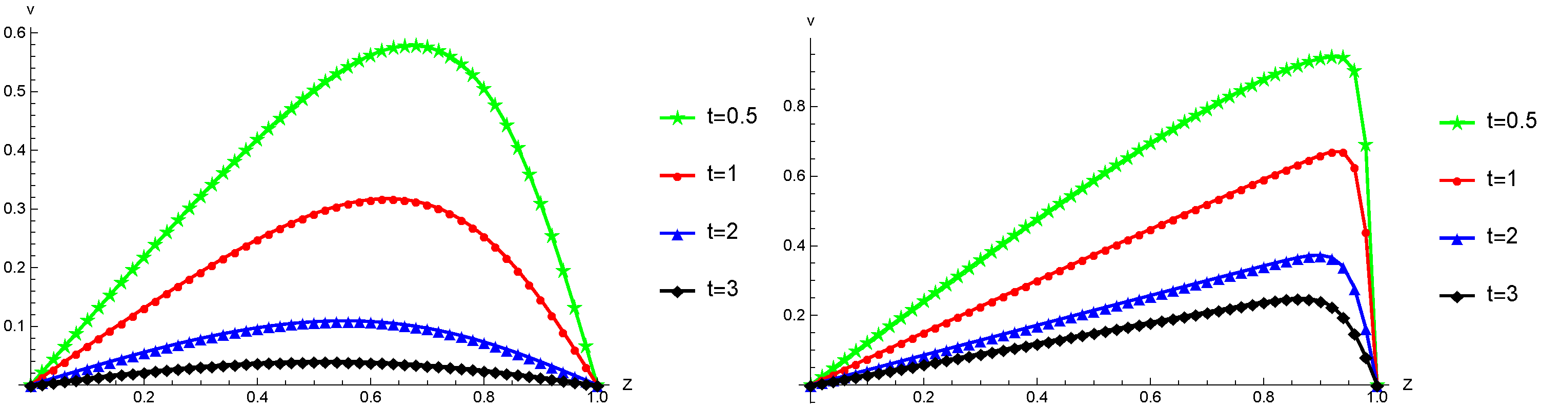
Figure 1.
The computed numerical solutions (depicted as diamonds, triangles, circles, and stars) and the exact solutions (illustrated as solid lines) are displayed with a step size of , a time increment of , and the parameters (in the left figure) and (in the right figure) for different time points in Example 1.
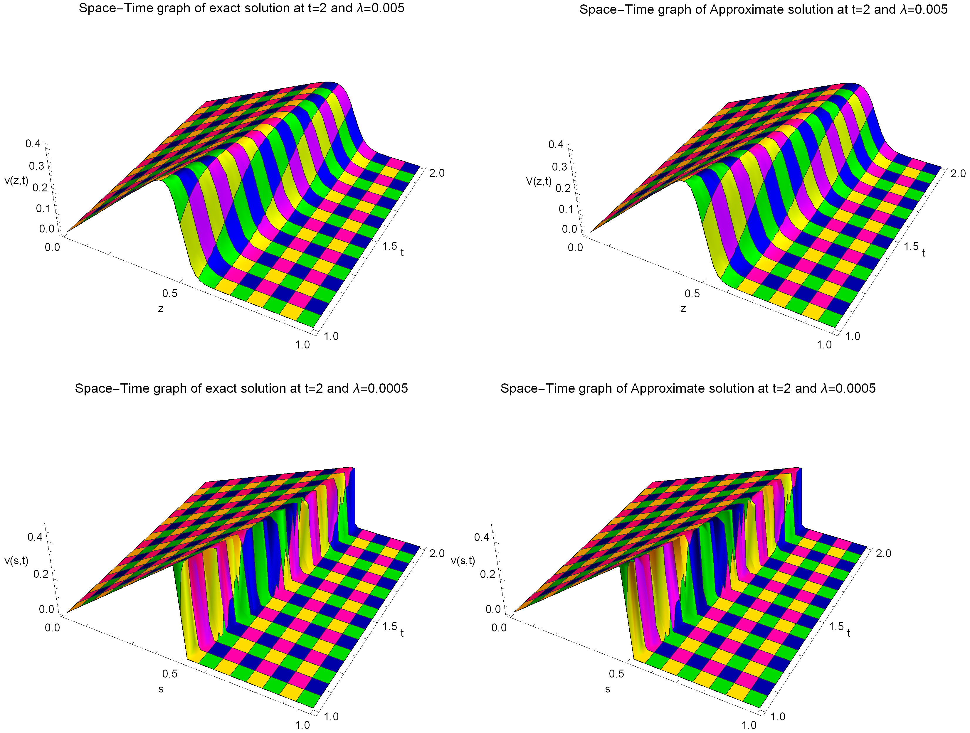
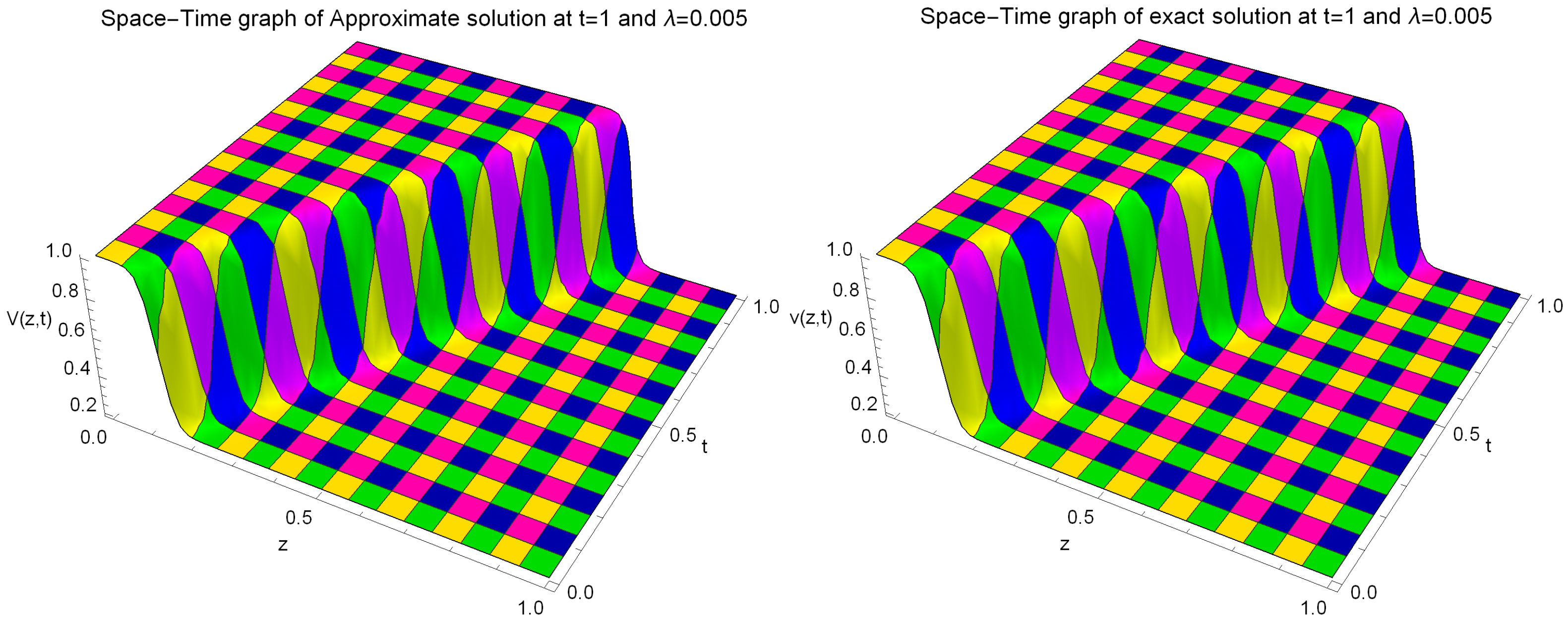
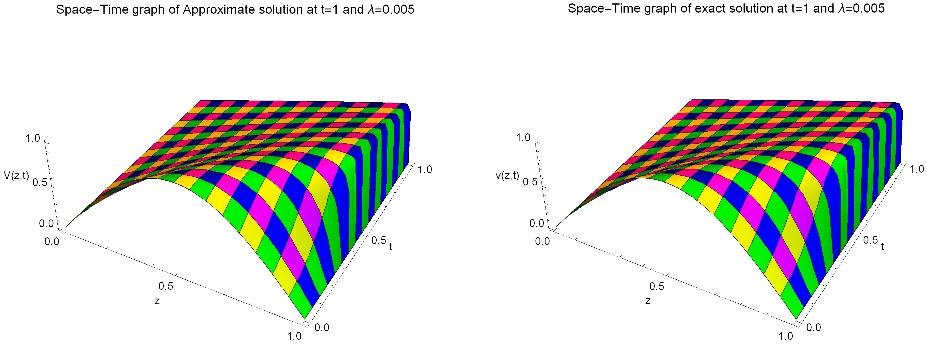
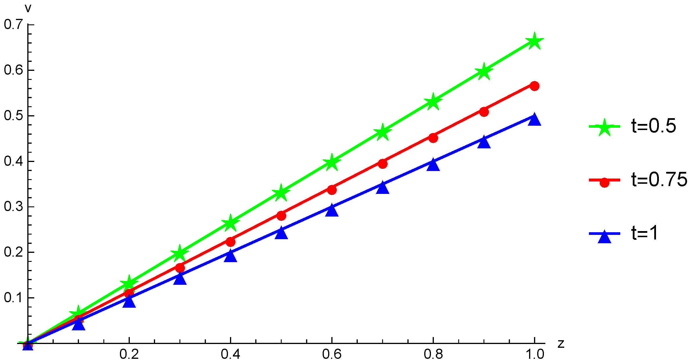
Figure 2.
The solutions obtained through numerical computation and the exact solutions for Example 1 are presented while considering the parameter values: and , along with two different values for , namely and .
Figure 2.
The solutions obtained through numerical computation and the exact solutions for Example 1 are presented while considering the parameter values: and , along with two different values for , namely and .
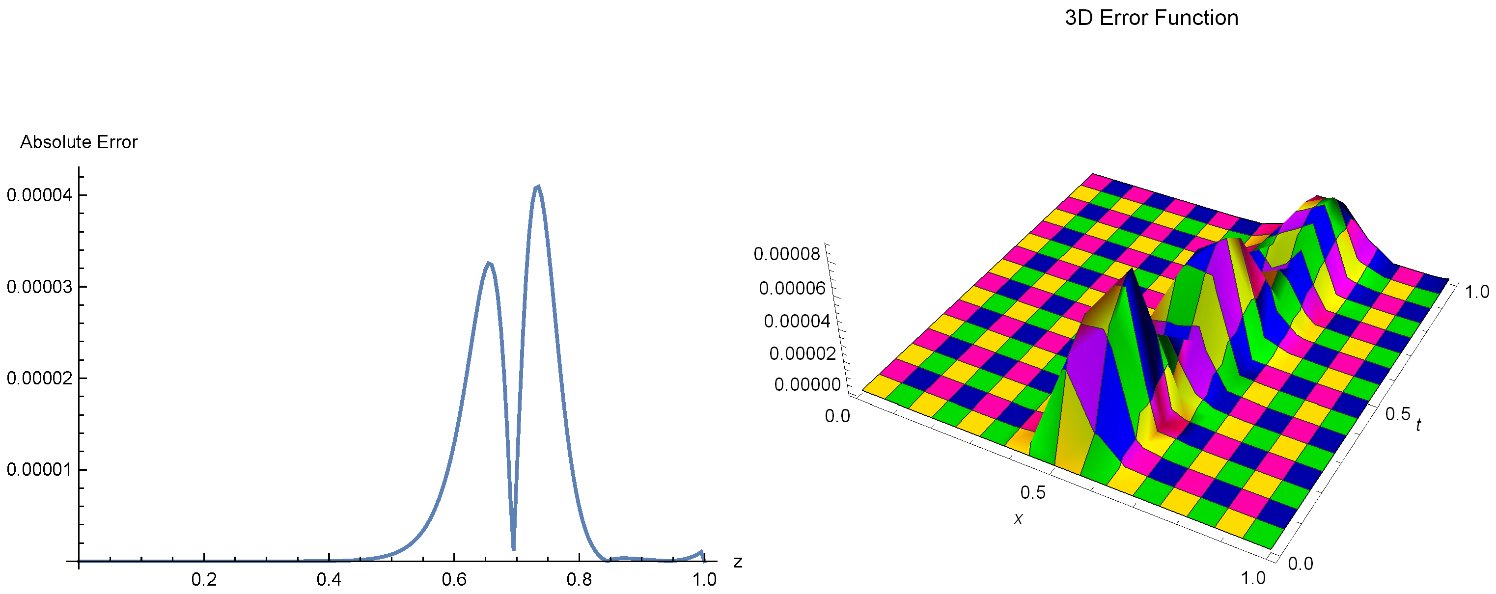
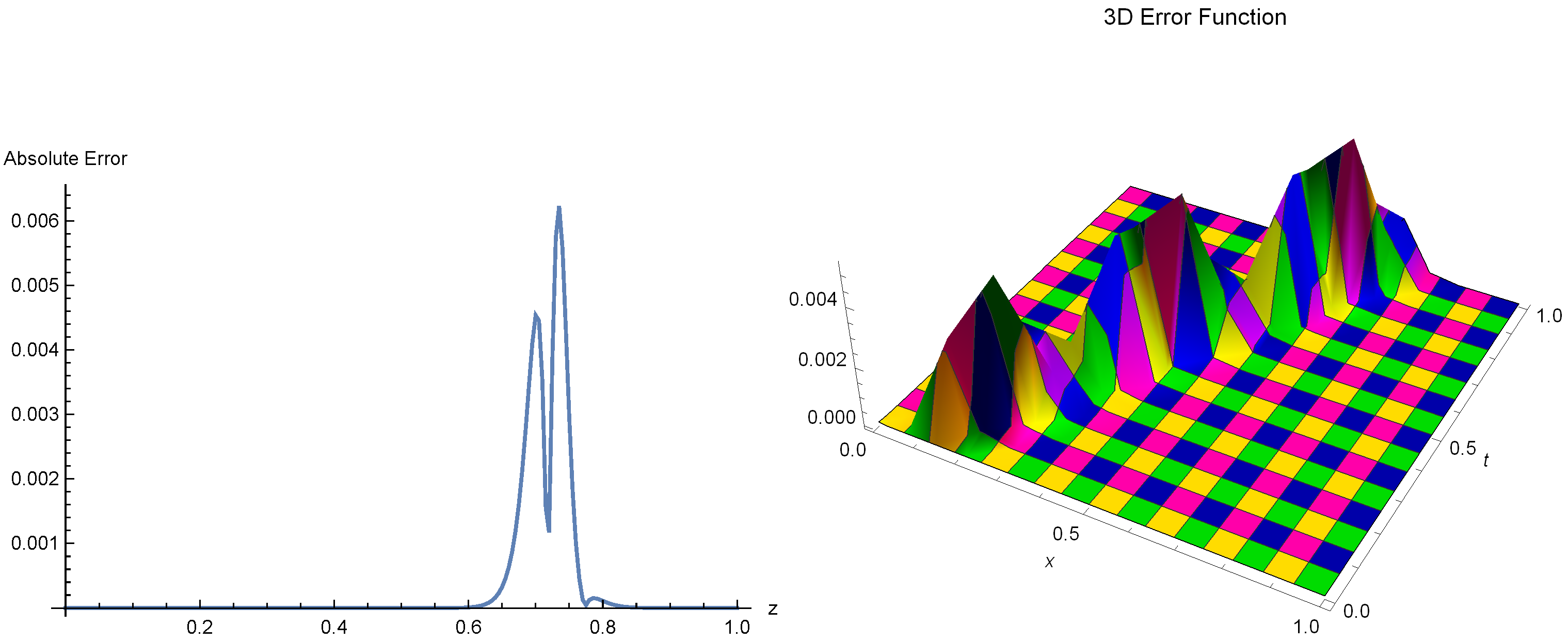
Figure 3.
The error distributions in both two-dimensional (2D) and three-dimensional (3D) settings at time are displayed for Example 1, where the step size is set to and the time increment is .
Figure 3.
The error distributions in both two-dimensional (2D) and three-dimensional (3D) settings at time are displayed for Example 1, where the step size is set to and the time increment is .
Figure 4.
The computed approximate solutions (depicted as triangles, circles, and stars) and the corresponding exact solutions (illustrated as solid lines) for Example 2 are displayed across various time instances, considering the following parameter values: , , and .
Figure 4.
The computed approximate solutions (depicted as triangles, circles, and stars) and the corresponding exact solutions (illustrated as solid lines) for Example 2 are displayed across various time instances, considering the following parameter values: , , and .
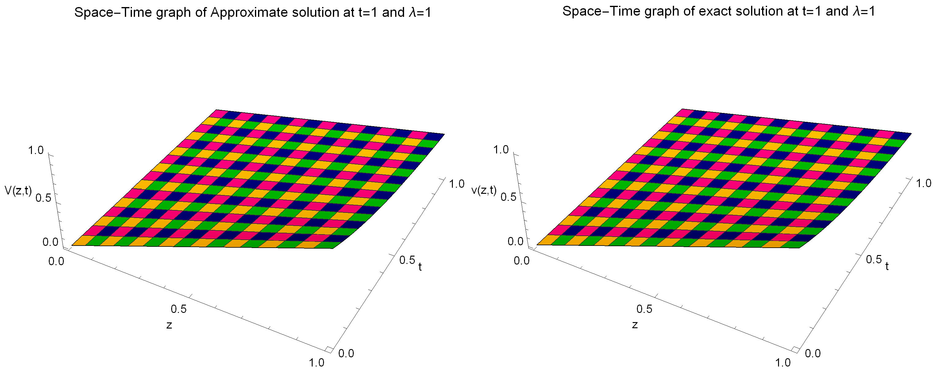
Figure 5.
The estimated solution (depicted on the left) and the precise solution (displayed on the right) are presented with the following parameter values: , , , and for Example 2.
Figure 5.
The estimated solution (depicted on the left) and the precise solution (displayed on the right) are presented with the following parameter values: , , , and for Example 2.
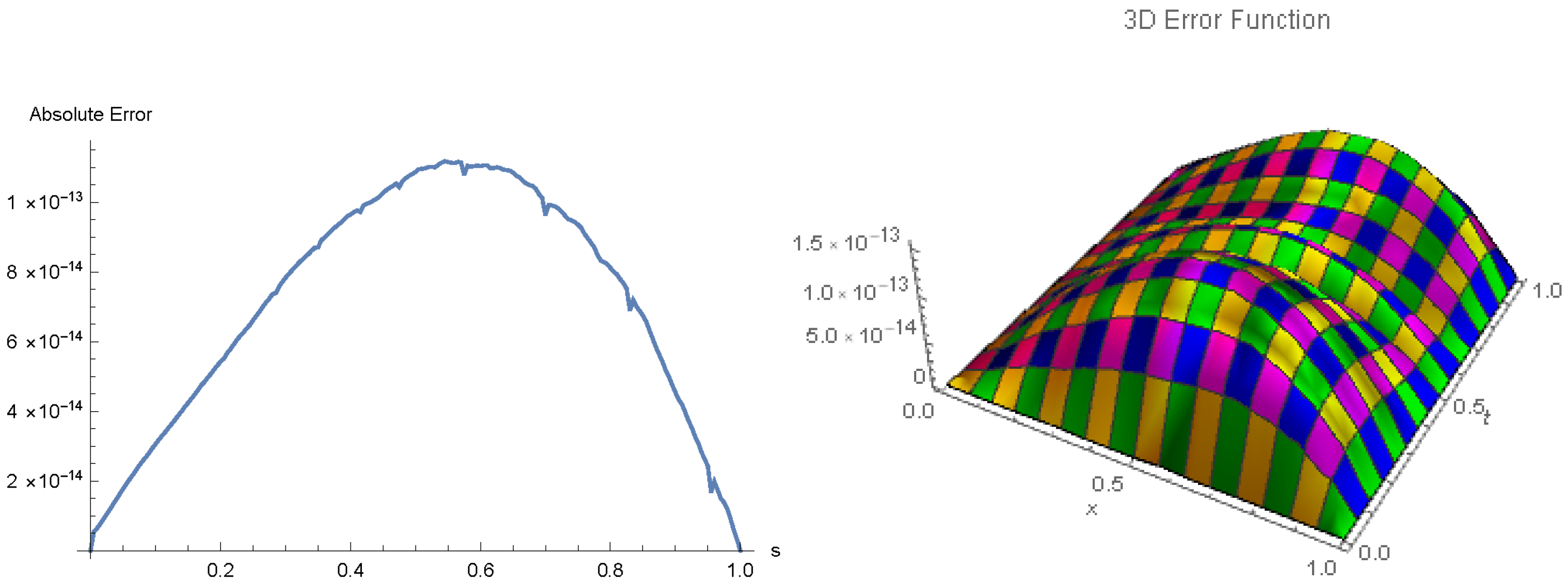
Figure 6.
The error distributions in both two-dimensional (2D) and three-dimensional (3D) contexts for Example 2 are shown, employing the parameters and .
Figure 6.
The error distributions in both two-dimensional (2D) and three-dimensional (3D) contexts for Example 2 are shown, employing the parameters and .
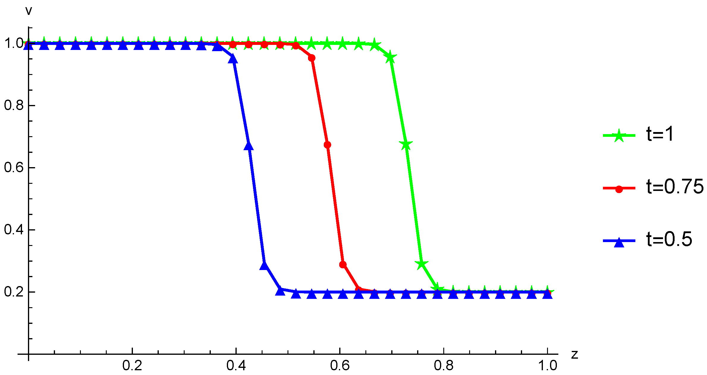
Figure 7.
The computed numerical solutions (indicated by triangles, circles, and stars) and the corresponding exact solutions (shown as solid lines) are presented for Example 3. These are displayed for two cases: one with and (in the left figure), and another with (in the right figure), across various time points.
Figure 8.
The estimated solution (on the left) and the precise solution (on the right) for Example 3 are presented with parameter values of , , and .
Figure 8.
The estimated solution (on the left) and the precise solution (on the right) for Example 3 are presented with parameter values of , , and .
Figure 9.
The computed numerical solutions (indicated by triangles, circles, and stars) and the corresponding exact solutions (depicted as solid lines) for Example 4 are presented across various time points, considering the following parameters: and .
Figure 9.
The computed numerical solutions (indicated by triangles, circles, and stars) and the corresponding exact solutions (depicted as solid lines) for Example 4 are presented across various time points, considering the following parameters: and .
Figure 10.
The estimated solution (on the left) and the accurate solution (on the right) for Example 4 are presented with parameter values of , , and .
Figure 10.
The estimated solution (on the left) and the accurate solution (on the right) for Example 4 are presented with parameter values of , , and .
Figure 11.
The error distributions in both two-dimensional (2D) and three-dimensional (3D) contexts for Example 4 are displayed under the conditions of , , and .
Figure 11.
The error distributions in both two-dimensional (2D) and three-dimensional (3D) contexts for Example 4 are displayed under the conditions of , , and .
Table 1.
The computed numerical solutions for Example 1 are shown at various time instances with the parameter , an interval of , a step size of , and a time increment of .
Table 1.
The computed numerical solutions for Example 1 are shown at various time instances with the parameter , an interval of , a step size of , and a time increment of .
| z | | | | | | |
|---|
| - | CBS [24] | Present | Exact | | CBS [24] | Present | Exact | | CBS [24] | Present | Exact | |
| 0.1 | 0.05883 | 0.05882 | 0.05882 | | 0.04000 | 0.04000 | 0.04000 | | 0.03077 | 0.03077 | 0.03077 | |
| 0.2 | 0.11765 | 0.11765 | 0.11766 | | 0.08000 | 0.08000 | 0.08000 | | 0.06154 | 0.06154 | 0.06154 | |
| 0.3 | 0.17648 | 0.17647 | 0.17647 | | 0.12001 | 0.12000 | 0.12000 | | 0.09231 | 0.09231 | 0.09231 | |
| 0.4 | 0.23531 | 0.23529 | 0.23529 | | 0.16001 | 0.16000 | 0.16000 | | 0.12308 | 0.12308 | 0.12308 | |
| 0.5 | 0.29414 | 0.29412 | 0.29412 | | 0.20001 | 0.20000 | 0.20000 | | 0.15385 | 0.15385 | 0.15385 | |
| 0.6 | 0.35296 | 0.35294 | 0.35294 | | 0.24001 | 0.24000 | 0.24000 | | 0.18462 | 0.18462 | 0.18462 | |
| 0.7 | 0.00000 | 0.00000 | 0.00000 | | 0.28001 | 0.28000 | 0.28000 | | 0.21539 | 0.21538 | 0.21538 | |
| 0.8 | 0.00000 | 0.00000 | 0.00000 | | 0.00811 | 0.00925 | 0.00976 | | 0.24616 | 0.24615 | 0.24615 | |
| 0.9 | 0.00000 | 0.00000 | 0.00000 | | 0.00000 | 0.00000 | 0.00000 | | 0.12358 | 0.12435 | 0.12435 | |
| CPU time | | 1.51563 | | | | 3.23438 | | | | 4.90625 | | |
Table 2.
The error magnitudes for Example 1 were computed with the parameter , a step size of , and a time increment of at various time instances.
Table 2.
The error magnitudes for Example 1 were computed with the parameter , a step size of , and a time increment of at various time instances.
| Ref. | | | | | | |
|---|
| | | | | | | | | | |
|---|
| [21] | | | | | | | | | |
| [22] | | | | | | | | | |
| QBCM [25] | | | | | | | | | |
| CBCM [25] | | | | | | | | | |
| Present | | | | | | | | | |
| CPU time | | | | | | | | | |
Table 3.
The error magnitudes for Example 1 were calculated for different time points using the parameter , a step size of , and a time increment of .
Table 3.
The error magnitudes for Example 1 were calculated for different time points using the parameter , a step size of , and a time increment of .
| Ref. | | | | | | |
|---|
| | | | | | | | | | |
|---|
| [21] | | | | | | | | | |
| [22] | | | | | | | | | |
| QBCM [25] | | | | | | | | | |
| CBCM [25] | | | | | | | | | |
| Present | | | | | | | | | |
| CPU time | | | | | | | | | |
Table 4.
The convergence rate assessment was conducted for various values of N in Example 1 by considering the following parameters: , , and .
Table 4.
The convergence rate assessment was conducted for various values of N in Example 1 by considering the following parameters: , , and .
| N | | Ratio | Order of Convergence | CPU Time |
|---|
| 25 | | – | – | 0.171875 |
| 50 | | | | 0.34375 |
| 100 | | | | 0.890625 |
| 200 | | | | 2.26563 |
| 400 | | | | 8.28125 |
Table 5.
The computed numerical solutions for Example 2 are obtained with the given parameter values: , , and .
Table 5.
The computed numerical solutions for Example 2 are obtained with the given parameter values: , , and .
| | | | |
|---|
| z | Present | [37] | [22] | Exact | | z | Present | [37] | [22] | Exact | |
|---|
| | 0.3082 | 0.9928 | 0.9943 | 0.9953 | 0.9926 | | 0.7841 | 0.9937 | 0.9974 | 0.9942 | 0.9937 | |
| | 0.3542 | 0.9563 | 0.9570 | 0.9609 | 0.9555 | | 0.8339 | 0.9564 | 0.9613 | 0.9575 | 0.9560 | |
| | 0.3809 | 0.8844 | 0.8849 | 0.8844 | 0.8830 | | 0.8618 | 0.8804 | 0.8885 | 0.8812 | 0.8793 | |
| | 0.4030 | 0.7673 | 0.7699 | 0.7670 | 0.7655 | | 0.8844 | 0.7559 | 0.7703 | 0.7576 | 0.7561 | |
| | 0.4456 | 0.4453 | 0.4484 | 0.4446 | 0.4439 | | 0.9245 | 0.4521 | 0.4645 | 0.4512 | 0.4515 | |
| | 0.4632 | 0.3435 | 0.3484 | 0.3451 | 0.3426 | | 0.9371 | 0.3746 | 0.3850 | 0.3757 | 0.3735 | |
| | 0.4824 | 0.2735 | 0.2788 | 0.2742 | 0.2732 | | 0.9495 | 0.3156 | 0.3244 | 0.3134 | 0.3154 | |
| | 0.5076 | 0.2284 | 0.2331 | 0.2279 | 0.2283 | | 0.9631 | 0.2701 | 0.2779 | 0.2779 | 0.2713 | |
| | 0.5520 | 0.2049 | 0.2087 | 0.2044 | 0.2049 | | 0.9791 | 0.2346 | 0.2431 | 0.2463 | 0.2393 | |
| CPU time | 4.8125 | | | | | | 12.078 | | | | |
Table 6.
The computed numerical solutions for Example 2 were derived by considering the following parameters: , time , and interval .
Table 6.
The computed numerical solutions for Example 2 were derived by considering the following parameters: , time , and interval .
| z | Present | Present | CBS [24] | CBS [24] | PGM [20] | PY [20] | CD [20] | QBGT [28] | Exact |
|---|
| | | | | | | | | | |
|---|
| | | | | | | | | | |
|---|
| 0.056 | 1.000 | | | 1.000 | | | 1.030 | | |
| 0.111 | 1.000 | | | 1.000 | | | 0.990 | | |
| 0.167 | 1.000 | | | 1.000 | | | 1.009 | | |
| 0.278 | 0.999 | | | 0.996 | | | 1.004 | | |
| 0.333 | 0.983 | | | 0.994 | | | 0.986 | | |
| 0.389 | 0.852 | | | 0.835 | | | 0.696 | | |
| 0.444 | 0.449 | | | 0.461 | | | 0.360 | | |
| 0.500 | 0.238 | | | 0.240 | | | 0.228 | | |
| 0.556 | 0.204 | | | 0.199 | | | 0.203 | | |
| 0.611 | 0.200 | | | 0.199 | | | 0.200 | | |
| 0.667 | 0.200 | | | 0.200 | | | 0.200 | | |
| 0.722 | 0.200 | | | 0.200 | | | 0.200 | | |
| 0.778 | 0.200 | | | 0.200 | | | 0.200 | | |
| 0.833 | 0.200 | | | 0.200 | | | 0.200 | | |
| 0.889 | 0.200 | | | 0.200 | | | 0.200 | | |
| 0.944 | 0.200 | | | 0.200 | | | 0.200 | | |
| CPU time | 0.063 | 0.672 | | | | | | | |
Table 7.
The convergence rate assessment for Example 2 was conducted at time , considering the various values of N while maintaining .
Table 7.
The convergence rate assessment for Example 2 was conducted at time , considering the various values of N while maintaining .
| N | | Ratio | Order of Convergence | CPU Time |
|---|
| 16 | | – | – | 0.10938 |
| 32 | | | | 0.21875 |
| 64 | | | | 0.56250 |
| 128 | | | | 1.26563 |
| 256 | | | | 4.79688 |
Table 8.
A contrast of the solutions at different positions was performed for Example 3 at time , utilizing parameters and .
Table 8.
A contrast of the solutions at different positions was performed for Example 3 at time , utilizing parameters and .
| z | | | | | | | | | | |
|---|
| | CBS [24] | Present | CBS [24] | Present | CBS [24] | Present | CBS [24] | Present | CBS [24] | Present | Exact |
|---|
| 0.1 | 0.10888 | | | | 0.10954 | | | | | 0.10952 | | | | | |
| 0.2 | 0.20847 | | | | 0.20979 | | | | | 0.20975 | | | | | |
| 0.3 | 0.28992 | | | | 0.29190 | | | | | 0.29184 | | | | | |
| 0.4 | 0.34537 | | | | 0.34792 | | | | | 0.34785 | | | | | |
| 0.5 | 0.36859 | | | | 0.37158 | | | | | 0.37149 | | | | | |
| 0.6 | 0.35589 | | | | 0.35905 | | | | | 0.35896 | | | | | |
| 0.7 | 0.30696 | | | | 0.30990 | | | | | 0.30983 | | | | | |
| 0.8 | 0.22552 | | | | 0.22782 | | | | | 0.22776 | | | | | |
| 0.9 | 0.11942 | | | | 0.12069 | | | | | 0.12065 | | | | | |
| CPU time | | 09.9242 | | | 21.4764 | | | 39.2374 | | | 103.675 | | | 237.885 | |
Table 9.
The estimated solutions for Example 3 were computed by using a step size of and a time increment of , considering various values of .
Table 9.
The estimated solutions for Example 3 were computed by using a step size of and a time increment of , considering various values of .
| z | t | | | | | | |
|---|
| - | - | CBS [24] | Present | Exact | CBS [24] | Present | Exact | CBS [24] | Present | Exact | CPU |
|---|
| 0.25 | 0.4 | | | 0.01357 | | | | 0.30889 | | | | | 43.7382 |
| | 0.6 | | | 0.00189 | | | | 0.24074 | | | | | 62.5638 |
| | 0.8 | | | 0.00026 | | | | 0.19568 | | | | | 84.5875 |
| | 1.0 | | | 0.00004 | | | | 0.16256 | | | | | 143.657 |
| | 3.0 | | | 0.00000 | | | | 0.02720 | | | | | 332.875 |
| 0.50 | 0.4 | | | 0.01924 | | | | 0.56963 | | | | | 43.7382 |
| | 0.6 | | | 0.00267 | | | | 0.44721 | | | | | 62.5638 |
| | 0.8 | | | 0.00037 | | | | 0.35924 | | | | | 84.5875 |
| | 1.0 | | | 0.00005 | | | | 0.29192 | | | | | 143.657 |
| | 3.0 | | | 0.00000 | | | | 0.04021 | | | | | 332.875 |
| 0.75 | 0.4 | | | 0.01363 | | | | 0.62544 | | | | | 43.7382 |
| | 0.6 | | | 0.00189 | | | | 0.48721 | | | | | 62.5638 |
| | 0.8 | | | 0.00026 | | | | 0.37392 | | | | | 84.5875 |
| | 1.0 | | | 0.00004 | | | | 0.28747 | | | | | 143.657 |
| | 3.0 | | | 0.00000 | | | | 0.02977 | | | | | 332.875 |
Table 10.
Error magnitudes for Example 4 at time are evaluated across various values of N while maintaining .
Table 10.
Error magnitudes for Example 4 at time are evaluated across various values of N while maintaining .
| N | CuTBS [39] | | Present Scheme | |
|---|
| | | | | | OC | CPU |
|---|
| 10 | | | | | | – | 0.07813 |
| 20 | | | | | | 2.00000 | 0.14063 |
| 40 | | | | | | 1.77259 | 0.31250 |
| 80 | | | | | | 1.99559 | 0.76563 |
| 100 | | | | | | 2.11664 | 0.92188 |

 ,
, 
