Abstract
Brilleslyper et al. investigated how the number of zeros of a one-parameter family of harmonic trinomials varies with a real parameter. Brooks and Lee obtained a similar theorem for an analogous family of harmonic trinomials with poles. In this paper, we investigate the number of zeros of convex combinations of members of these families and show that it is possible for a convex combination of two members of a family to have more zeros than either of its constituent parts. Our main tool to prove these results is the harmonic analog of Rouché’s theorem.
MSC:
30C15
1. Introduction
A complex-valued harmonic function on a simply connected domain D in has the form
for analytic functions h and g, where is called the co-analytic part of f. We are especially interested in the case in which h and g are polynomials. Whereas the number of zeros of a non-constant analytic polynomial is always equal to its degree, the situation for harmonic polynomials is more complicated. In particular, for f as in (1), the number of zeros is not a simple function of the degrees of h and g and depends on the coefficients. Some of the first results about harmonic polynomials sought to determine a sharp bound on the number of zeros in terms of the degrees of h and g. If the degree of h is n and the degree of g is k, where , then a reasonable expectation is that the maximum number of zeros of f is . Sheil-Small [1] made this conjecture, and it was later shown to be correct [2,3,4]. A natural extension is to consider the more restrictive case in which . In this case, Wilmshurst [4] conjectured that the maximum number of zeros of f is . Khavinson and Swiatek [5] proved this conjecture for , but Lee et al. [6] later showed it is not true in general.
Because the number of zeros of a harmonic polynomial is not a simple function of the degrees of the analytic and co-analytic parts, several researchers have turned their attention to a detailed study of specific families of harmonic functions. They have sought to determine the maximum and minimum number of zeros, how the number of zeros varies with the coefficients, and the location of these zeros. See [7,8,9,10,11,12,13,14,15]. We discuss several of their results in some detail because they are the motivation for the current work.
In [9,10], the authors considered a one-parameter family of trinomials. Although they determined precisely how the number of zeros varies with the parameter, a corollary of their main theorem is as follows:
Corollary 1
([9,10]). Suppose with and , and let
Then has a maximum of zeros, obtained for all sufficiently large .
Remark 1.
The proof given in [9] shows that attains this maximum of zeros for all . For all of the results stated below, it is similarly possible to make precise what “sufficiently large” and “sufficiently small” mean. However, the thresholds are complicated expressions that are not illuminating.
Brooks and Lee [12] carried out a similar detailed analysis of an analogous one-parameter family of harmonic functions with poles. A corollary of their main theorem is as follows:
Corollary 2.
Suppose with and , and let
Then
- 1.
- has a maximum of zeros, obtained when is sufficiently small; and
- 2.
- has a minimum of zeros, obtained when is sufficiently large.
We wish to understand the zeros of more complicated harmonic functions. We might naturally ask: if we understand the zeros of some simple families of harmonic functions, can we use this information to make conclusions about more complicated families constructed from these simple pieces? In this paper, we study convex combinations of members of families (2) and (3). Thus we study
and
Although one might conjecture that once we fix all exponents, the maximum number of zeros for a convex combination is the larger of the maximum number of zeros for the constituent pieces, we prove that there are choices of the parameters for which the convex combination has strictly more zeros than either piece. This result is rather surprising. Before we state our theorems precisely, we consider two examples of this phenomenon.
Example 1.
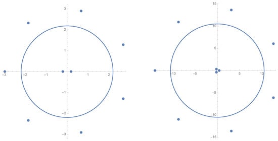
Consider
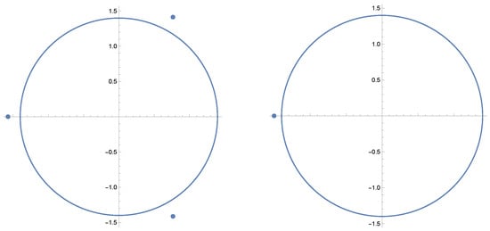
If we take and , we are in the situation described in Corollary 1, in which the two trinomials making up the convex combination have the maximum number of zeros of and . These zeros are shown in Figure 1.
Figure 1.
The zeros and critical curve for (left) and (right).
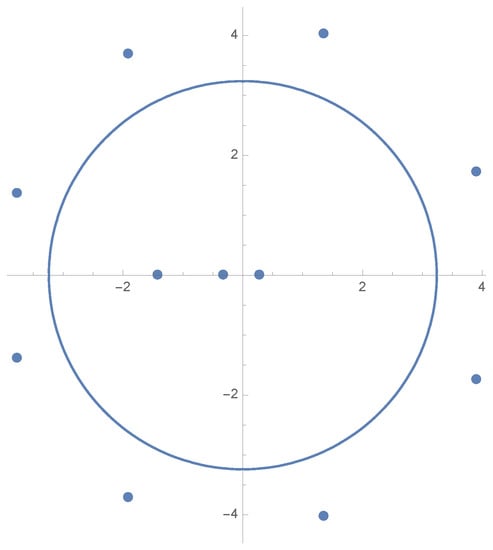
However, the convex combination has 11 zeros, as shown in Figure 2.
Figure 2.
The zeros and critical curve for .
Example 2.
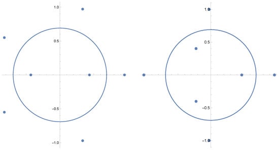
Next, consider
Take and vary b. First, consider . For such a and b, the first part of Corollary 2 applies, and each piece making up the convex combination has zeros. See Figure 3. However, for , the convex combination has 8 zeros. See Figure 4.
Figure 3.
The zeros and critical curve of (left) and (right) for .
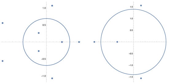
Figure 4.
The zeros and critical curve of as in Example 2 for (left) and (right).
Now consider . The second part of Corollary 2 now applies; the numbers of zeros of the constituent pieces of the convex combination are and , respectively. See Figure 5. However, the convex combination itself has 4 zeros for b (and, in fact, for all sufficiently large b), displaying different behavior compared to its constituent parts. See Figure 4.
Figure 5.
The zeros and critical curve of (left) and (right) for .
Our two main theorems illustrate that these are not isolated examples; in fact, there are large subfamilies of (4) and (5) exhibiting this interesting behavior.
Theorem 1.
Let
Let satisfy and . Let and . Then, there exists , such that for all has zeros.
Theorem 2.
Let
Let satisfy and . Let and . Then there exist and , such that
- (1)
- For all , has zeros.
- (2)
- For all , has zeros.
2. Background and Set-Up
In this section, we state all the definitions and theorems needed for the proofs of the theorems, in particular, Rouché’s theorem for harmonic functions with poles. We also study some basic properties of the subfamilies of (4) and (5) considered in Theorems 1 and 2.
2.1. Definitions and Tools
One of the most useful tools for studying zeros of analytic functions is Rouché’s theorem, which allows one to count the zeros of a given function inside a simple closed curve C by comparing it to a function whose zeros are understood. An analog of this theorem exists for harmonic functions with poles. In order to state it, we must first understand more about the geometry of harmonic functions and how zeros and poles are counted.
An analytic function h on a domain D is sense-preserving. Thus, if C is a simple, closed, positively oriented contour in D whose interior lies entirely in D, its image under h remains positively oriented. A co-analytic function, on the other hand, is sense-reversing. Because a harmonic function is the sum of an analytic function and a co-analytic function, it is, in general, sense-preserving in some parts of its domain and sense-reversing in others. The complex dilatation allows us to identify these regions.
Definition 1.
Let be a harmonic function on D, with h and g analytic on D. The complex dilatation is the function ω defined by
The key fact about the complex dilatation is contained in the following well-known proposition.
Proposition 1.
Let be harmonic on D, with complex dilatation ω.
- 1.
- If throughout some region , then f is sense-preserving on R.
- 2.
- If on , then f is sense-reversing on R.
The set of points at which is called the critical curve for f.
The sense-preserving and sense-reversing regions are important because they play a role in the definitions of the order of a zero and the order of a pole. More specifically, the sign of the order of a zero or a pole depends on whether it is in the sense-preserving region (positive order) or the sense-reversing region (negative order). See [11] for a more detailed discussion of why this convention makes sense. For this paper, we take the following to be our definitions of the order of a zero and the order of a pole.
Definition 2
([16]). Let be a complex-valued harmonic function and suppose . Write
If is in a sense-preserving region, we define the order of to be r and if is in a sense-reversing region, we define its order to be . If is on the critical curve, we call it a singular zero and its order is not defined.
Definition 3
([17]). Let f be a harmonic function on a domain except at a finite number of poles. Suppose that the local representation of f around a pole is
for some constant A, and where r and s are finite.
- (i)
- If for some and , or with , then f is sense-preserving near and f has a pole at of order r.
- (ii)
- If for some and , or with , then f is sense-reversing near and f has a pole at of order .
With this background, we can state the main tool we need to prove our theorems, which is the harmonic analog of Rouché’s theorem. The theorem allows us to relate the sums of the orders of zeros and poles of two functions within a simple closed curve C provided a certain inequality is satisfied on C. In the statement of the theorem and throughout the rest of the paper, we let denote the sum of the orders of the zeros of p in C and we let denote the sum of the orders of the poles of p in C.
Theorem 3
(Rouché’s theorem for harmonic functions). Let p and q be harmonic, except for a finite number of poles, in a simply connected domain . Let C be a simple, closed curve contained in D. If at each point on C, and if p and q have no poles on C and no singular zeros in C, then .
2.2. The Subfamilies
Although studying families (4) and (5) for all positive a and b and all would be potentially interesting, it would also be extremely difficult. A large part of the difficulty comes from the fact that, for most choices of a, b, and s, the critical curve for the function is quite complicated. Thus, as we seek to address the question of how the maximum number of zeros of a convex combination relates to the maximum numbers of zeros for the constituent pieces, it is reasonable to begin by studying subfamilies for which the critical curve is particularly simple.
Several different conditions on the parameters will yield a complex dilatation of the form
Note that is a composition of a Möbius transformation and a power function. This function is subordinate to the Möbius transformation as it also sends circles to circles. Even so, in general, the critical curve will be complicated. If, however, we require A to be 1, then the dilatation will reduce to and the critical curve will be precisely a circle. We now derive a set of conditions on the parameters for each family leading to this desirable form.
We begin with the complex dilatation of the first family (7). Factoring out of the numerator and out of the denominator gives
In order for the rational function in parentheses to have the form , we require
or, equivalently,
If we further require A to be 1, then
or, equivalently,
In order to apply Corollaries 1 and 2, we require and . Without loss of generality, we also assume that . Together with the first condition in (11), we obtain a strict ordering of the exponents
With this strict ordering, , we rewrite the dilatation as
The following proposition summarizes the properties of the subfamily of (4) considered in Theorem 1.
Proposition 2.
Let be as in (4). Let satisfy and . Let and .
- 1.
- 2.
- The critical curve is a circle, , centered at the origin with radius .
- 3.
- The region inside the critical curve is sense-reversing.
- 4.
- The region outside the critical curve is sense-preserving.
We now consider the complex dilatation of the second family (8). We again desire this dilatation to be of the form given in (9). Factoring out of the numerator and out of the denominator gives
In order for the rational function in parentheses to have the form , we require
The first condition is equivalent to
If we further require A to be 1, then
or, equivalently,
With this form of s, the condition that is equivalent to
Therefore, the conditions for the subfamily of (5) are the same as the conditions for the subfamily of (4). The same strict ordering of the exponents (13) also applies to this subfamily. With these conditions, the dilatation simplifies to
The following proposition summarizes the properties of the subfamily of (5) considered in Theorem 2.
Proposition 3.
Let be as in (5). Let satisfy and . Let and .
- 1.
- 2.
- The critical curve is a circle, , centered at the origin with radius .
- 3.
- The region inside the critical curve is sense-reversing.
- 4.
- The region outside the critical curve is sense-preserving.
We are now ready to proceed with the proofs of Theorems 1 and 2.
3. Proof of Theorem 1
In order to prove Theorem 1, we determine the sum of the orders of the zeros of in and within the critical curve for large values of b. With this information and an understanding of the sense-reversing and sense-preserving regions, we deduce the number of zeros of for large b. Due to the restrictions we impose on that fix s and make a a function of b once the exponents are fixed, will be referred to as for the rest of this section.
Lemma 1.
The sum of the orders of the zeros of in is m.
Proof.
We prove this lemma by proving that the sum of the orders of the zeros of inside a circle of a sufficiently large radius R is m. We prove this latter statement using Rouché’s theorem to compare the zeros of to the zeros of . If , then because , and because the natural number m exceeds and ℓ,
If also , then
It is easy to check that, because , . Thus, if , then for all with
By Rouché’s theorem, the sum of the orders of the zeros for inside the circle of radius R is the same as the sum of the orders of the zeros for p. Since p has a zero of order m at the origin, the sum of the orders of the zeros of inside the circle is m, for all sufficiently large R. □
Now, we find the sum of the orders of the zeros inside the critical curve.
Lemma 2.
For sufficiently large b, the sum of the orders of the zeros of inside the critical curve is .
Proof.
We prove this lemma using Rouché’s theorem. We show that has the same sum of the orders of zeros as inside of the critical curve; that is, we show
for all z on the critical curve. Equation (20) will follow if we show
is greater than zero for all z on the critical curve. Since points on the critical curve satisfy , (21) is equivalent to
By factoring out and using and to simplify the second term, (21) is equivalent to
The third term can also be simplified using , giving
This expression is positive if and only if the expression in square brackets is positive. Due to the relation between seen in (13), we find that the sum of the exponents on b in each term is negative. Indeed,
Therefore, each term involving b tends to 0 as b tends to infinity. Thus, there exists such that for all ,
Therefore, for such b,
It follows that p is the dominant term of on the critical curve, and by Rouché’s theorem, the sum of the orders of the zeros of inside its critical curve is the same as the sum of the orders of the zeros of p. Since p only has a zero of order located at the origin, the sum of the orders of the zeros of inside the critical curve is for sufficiently large b. □
Now, we have everything needed to prove Theorem 1.
Proof of Theorem 1.
By Lemma 1, the sum of the orders of the zeros of in is m. Since the inside of the critical curve is the sense-reversing region and the outside is the sense-preserving region, Lemma 2 gives that the sum of the orders of the zeros of in the sense-reversing region is . Therefore, the sum of the orders of the zeros of outside of the critical curve is , and the total number of zeros for is . □
4. Proof of Theorem 2
We now turn to the family as given in (5), with the additional restrictions on the exponents and parameters given in the statement of Theorem 2. Thus, as above, s is now fixed, a is a function of b, and we abbreviate by . In order to count the zeros of in the complex plane, we first determine the sum of the orders of the zeros of , both in the plane and within the critical circle for small and large b.
Lemma 3.
The sum of the orders of the zeros of in is .
Proof.
We apply Rouché’s theorem to and on a circle centered at the origin with a sufficiently large radius R. Recalling that , we see that for ,
If we also take (which, as above, is greater than 1), then
Thus if , it follows that for all ; that is, for all z on . By Rouché’s theorem,
Because has a pole at the origin of order , we have . □
We now count the zeros inside the critical circle, , for small and large b. In conjunction with Lemma 3, this will allow us to calculate the total number of zeros, proving Theorem 2.
Proof of Theorem 2.
First, consider b to be small. In this case, we apply Rouché’s theorem to and on the critical circle, . Points on this circle satisfy , so on this circle,
We show that all powers of b in this last expression are positive. The powers of b in the first and second terms are clearly positive. The power of b in the fourth term is . Finally, because and , the power of b in the third term is
Because all powers of b are positive, the expression approaches 0 as . In particular, there exists , such that this final expression is less than 1 for all . Then for all and z on ,
By Rouché’s theorem,
and, thus, . Because there are zeros in the sense-reversing region and the sum of the orders of the zeros in is , there are m zeros in the sense-preserving region. Then there are total zeros for .
We now consider b large. We apply Rouché’s theorem to and on the critical circle, . If , then on this circle,
Note that the expression in square brackets is positive.
On the other hand, on the critical curve,
Because , this expression is positive. Furthermore, implies that . Together, these facts imply that there is some , such that for all ,
Then for all , for z on ,
By Rouché’s theorem, then, .
One readily computes that is also the critical curve for p. A straight-forward calculation in the polar coordinates shows that all the zeros of p lie on a circle whose radius exceeds that of the critical circle; thus, p has no zeros inside . Because it has a pole of order at the origin,
Then , or, equivalently, . Because the sum of the orders of the zeros of in is , there are zeros in the sense-preserving region, giving a total of zeros for . □
5. Future Directions
This paper does not provide a detailed analysis of families (4) and (5) but only considers subfamilies for which the complex dilatation has the very special form . Many interesting questions remain for future work:
- There are actually several inequivalent sets of conditions on the exponents m, k, n, ℓ, and the parameters a, b, and s, for which the complex dilatation simplifies to , each leading to a different subfamily. Do these other subfamilies exhibit the same behaviors observed in our main theorems?
- Are there interesting results if we consider the convex combination
- Does anything interesting happen when we consider a convex combination of three terms, such aswhere for and ?
Author Contributions
Investigation, J.B., M.D. (Megan Dixon), M.D. (Michael Dorff), A.L. and R.O.; Writing—original draft, J.B., M.D. (Megan Dixon), M.D. (Michael Dorff), A.L. and R.O. All authors have read and agreed to the published version of the manuscript.
Funding
This research received no external funding.
Data Availability Statement
No new data were created for this research.
Conflicts of Interest
The authors declare no conflict of interest.
References
- Sheil-Small, T. Tagesbericht, Mathematisches Forsch. In Proceedings of the Funktionentheorie, Oberwolfach, Germany, 16–22 February 1992; p. 19. [Google Scholar]
- Bshouty, D.; Hengartner, W.; Suez, T. The exact bound on the number of zeros of harmonic polynomials. J. Anal. Math. 1995, 67, 207–218. [Google Scholar] [CrossRef]
- Peretz, R.; Schmid, J. Proceedings of the Ashkelon Workshop on Complex Function Theory; Bar-Ilan University: Ramat Gan, Israel, 1997; pp. 203–208. [Google Scholar]
- Wilmshurst, A.S. The valence of harmonic polynomials. Proc. Am. Math. Soc. 1998, 126, 2077–2081. [Google Scholar] [CrossRef]
- Khavinson, D.; Swiatek, G. On the maximal number of zeros of certain harmonic polynomials. Proc. Am. Math. Soc. 2003, 131, 409–414. [Google Scholar] [CrossRef]
- Lee, S.-Y.; Lerario, A.; Lundberg, E. Remarks on Wilmshurst’s theorem. Indiana Univ. Math. J. 2015, 64, 1153–1167. [Google Scholar] [CrossRef]
- Alemu, O.A.; Galeta, H.L. Curves formed by Vanishing Discriminant and Roots of Complex-valued Harmonic Polynomials (Computer-Aided Case Study). arXiv 2023, arXiv:2305.15548. [Google Scholar]
- Barrera, G.; Barrera, W.; Navarrete, J.P. On the number of roots for harmonic trinomials. J. Math. Anal. Appl. 2022, 514, 126313. [Google Scholar] [CrossRef]
- Brilleslyper, M.; Brooks, J.; Dorff, M.; Howell, R.; Schaubroeck, L. Zeros of a One-Parameter Family of Harmonic Trinomials. Proc. Am. Math. Soc. Ser. B 2020, 7, 82–90. [Google Scholar] [CrossRef]
- Brooks, J.; Dorff, M.; Hudson, A.; Pitts, E.; Whiffen, C.; Woodall, A. Zeros of a one-parameter family of harmonic trinomials. Bull. Malays. Math. Sci. Soc. 2022, 45, 1079–1091. [Google Scholar] [CrossRef]
- Brooks, J.; Dorff, M.; Muthuprakash, S.; Tanner, P. Zeros of several one-parameter families of harmonic functions. In Current Research in Mathematical and Computer Sciences IV; Lecko, A., Thomas, D.K., Eds.; Wydawnictwo UWM: Olsztyn, Poland, 2023. [Google Scholar]
- Brooks, J.; Lee, A. Zeros of a family of complex-valued harmonic functions with poles. 2023; submitted for publication. [Google Scholar]
- Galeta, H.L.; Alemu, O.A. Location of the zeros of certain complex valued harmonic polynomials. J. Math. 2022, 2022, 4886522. [Google Scholar]
- Gao, L.; Gao, J.; Liu, G. Location of the zeros of harmonic trinomials. Bull. Malays. Math. Sci. Soc. 2023, 46, 34. [Google Scholar] [CrossRef]
- Lundberg, E. The valence of harmonic polynomials viewed through the probabilistic lens. Proc. Am. Math. Soc. 2023, 151, 2963–2973. [Google Scholar] [CrossRef]
- Duren, P. Cambridge Tracts in Mathematics. In Harmonic Mappings in the Plane; Cambridge University Press: New York, NY, USA, 2004; p. 156. [Google Scholar]
- Suffridge, T.J.; Thompson, J.W. Local behavior of harmonic mappings. Complex Var. Elliptic Equ. 2000, 41, 63–80. [Google Scholar] [CrossRef]
Disclaimer/Publisher’s Note: The statements, opinions and data contained in all publications are solely those of the individual author(s) and contributor(s) and not of MDPI and/or the editor(s). MDPI and/or the editor(s) disclaim responsibility for any injury to people or property resulting from any ideas, methods, instructions or products referred to in the content. |
© 2023 by the authors. Licensee MDPI, Basel, Switzerland. This article is an open access article distributed under the terms and conditions of the Creative Commons Attribution (CC BY) license (https://creativecommons.org/licenses/by/4.0/).