Optimal Lot-Sizing Decisions for a Remanufacturing Production System under Spare Parts Supply Disruption

Abstract

Remanufacturing is one of the ways forward for product recovery initiatives and for maintaining sufficient production flow to satisfy customer demand by providing high-quality goods with a combination of new and return parts through a circular economy. Recently, manufacturers have been progressively incorporating remanufacturing processes, making their supply chains vulnerable to disruptions. One of the main disruptions that occurs in remanufacturing systems is the shortage of spare parts supply, which results in unexpected delays in the remanufacturing process and could eventually result in a possible loss of sales. In the event of such potential disruptions, remanufacturing facilities must manage their supply chains in an effective and optimal manner such that the negative impact of disruptions to their business can be minimised. In this study, a two-stage production–inventory system was analysed by developing a cost-minimisation model that focuses on the recovery schedule after the occurrence of a disruption in sourcing spare parts for a remanufacturer’s production cycle. The developed model was solved using the branch-and-bound algorithm, where the experimental results demonstrated that the model provides effective solutions. Through numerical experiments, results indicated that the optimal recovery schedule and the number of recovery cycles are considerably dependent on the disruption time, lost sales and backorder costs. A sensitivity analysis showed that the lost sales option seems to be more effective than the backorder sales option in optimising the system’s overall cost due to unmet demand, which becomes lost sales when serviceable items are reduced, thereby shortening recovery time. Furthermore, a case study revealed that a manufacturer’s response to disruption is highly influenced by the spare part costs and overall recovery costs as well as the supplier’s readiness level. The proposed model could assist managers in deciding the optimal production strategy whilst providing interesting managerial insights into vital spare parts recovery issues when disruption strikes.

1. Introduction

The circular economy contributes to achieving a sustainable society and economy by reducing resource consumption and waste generation. The notion of the circular economy becomes valid only when resources and value are reclaimed from products at their end-of-life (EOL) stages [1]. Products may undergo recycling, repair, reuse, refurbishing and remanufacturing after their disposal in the circular economy. Nevertheless, remanufacturing guarantees that the quality of remanufactured products is as good as that of new products with remarkably less energy consumption [2]. Remanufacturing and the closed-loop supply chain (CLSC) have a considerable influence on the environment and the economy. Remanufacturing is well known for its efficiency in closing the material flow loop, eliminating production waste, enhancing product life cycles, conserving energy and minimising processing costs [3,4].

Remanufacturing can be described as a method of returning used products to the state of new products; it involves collecting, inspecting, disassembling, cleaning, separating, repairing and assembling [5,6]. Remanufactured products can be sold for affordable costs, giving firms new sources of income. Customers frequently value the cost savings offered by refurbished goods. Additionally, remanufactured products can help businesses access new market groups, such as cost-conscious and environmentally conscious consumers. This process has been practised in a broad range of production industries, especially in the electronics and automotive sectors.

Given increased government legislation, social pressure and economic prospects, many companies have become involved in the remanufacturing industry. In addition, remanufacturing has arguably received more attention than traditional manufacturing operations and other processes, such as recycling. The direct benefits of remanufacturing are numerous; for instance, the energy consumed by remanufacturing processes is 85% lower than that consumed by manufacturing processes that produce an equivalent quantity of new products [2]. Furthermore, remanufacturing frequently uses less water than basic manufacturing processes, aiding in the conservation of this precious resource, especially in areas with scarce access to it. Remanufacturing also reduces carbon emissions, lowers the use of raw materials and enables the products to be sold at a 60% lower cost compared with new manufactured products [1,7]. This, in turn, delivers advantages to the community by providing job opportunities for unskilled and skilled workers, and it contributes to economic benefits through the reduced cost of remanufactured goods. Additionally, remanufacturing and closed-loop business strategies reduce the risks imposed by resource shortages, supply chain interruptions and shifting consumer preferences, hence enhancing long-term business resilience. The increasing need for remanufacturing due to these numerous advantages requires companies to organise their actions to explore and reap the full benefits of the coordination of forward and reverse material flows.

Nevertheless, the management of remanufacturing systems—particularly inventory plans—has always been a complicated task due to the growing interactions between various manufacturing and remanufacturing operations and uncertainty in the supply chain’s various stages. Inventory management in the remanufacturing process may be disrupted by several factors, including failure to identify production inventory during supply disruption [8,9], uncertain time taken to acquire specified components [10,11] and material flow and time control constraints in the production process [12,13,14].

The optimisation of remanufacturing efficiency when facing quality uncertainties can be improved via a basic assessment of system performance, integrating inventory and production planning, and resource allocation [15]. When dealing with demand uncertainty during production, fuzzy systems may aid in selection to enhance the effectiveness of sustainable inventory management and reduce the overall cost of the system [16]. Moreover, the effectiveness of control policies and the space required for the finished product are important at present to provide an enhanced comprehension of relations involving manufacturing, remanufacturing, and disposal activities [17]. Queuing systems for finished and returned products during demand uncertainty also has shown improvement in the inventory system [18]. Additionally, uncertainty in remanufacturing subsequently causes unexpected problems related to production planning, inventory management, network design and vehicle routing [19]. Logistics systems also play a crucial role in inventory management. Several aspects in logistics for remanufacturing systems that were studied include capacities of facilities [20], consignment stock policy [21], shipping policy [22], scheduling problems of capacitated products [23], inventory allocation [24], trade-in programs and return services [25,26]. Leuveano et al. [27] studied the inventory replenishment system in transportation and quality problems with consideration of the just-in-time (JIT) method.

Capacity planning in the reverse field, however, poses the following problems: somewhat uncertain market patterns, variability in the residence time of goods (the period a product lasts with its user until end of use), dependence on the quantity and timing of the end-of-use commodity returns on production and pricing patterns and uncertainty about the amount and timing of remanufactured product returns [28,29]. These specific features include a higher risk of shortages in end-of-use product returns because production can differ, and the dismantling level may be less than expected. This contributes to the overcapacity phenomena in selection and remanufacturing efficiency [30].

Remanufacturing is a feasible way to extend the useful life of a finished product or its parts. Despite its environmental, financial and social benefits, remanufacturing is correlated with many core problems linked to availability, scheduling and consistency (the used product or its parts). Regarding environmental preservation, Ghadimi et al. [31] practised the decision-making approach for suppliers in automotive spare parts as initiatives in adopting sustainability in supply chain management. Furthermore, Shi [32] established stochastic dynamic programs to solve the spare parts inventory control problem, where a sufficient supply of remanufactured parts was satisfied with the return of products. The interrelationships amongst installed bases, product returns and demand for spare parts contribute to optimal demand.

Spare parts availability is one of the main components in remanufacturing. Sourcing is difficult after spare parts production declines, whereas the rest of the operation remains long. Kurilova-Palisaitiene et al. [33] extensively discussed the contribution of lean production to shorter lead times. Spengler et al. [34] established policies of part recovery and spare parts supply for CLSC by developing a generic system dynamic model providing causes and effects in various forms of product take-back. Additionally, Ronzoni et al. [35] thoroughly investigated the aftermarket distribution channel for spare parts management when they developed a model considering the supply chain for automotive spare parts after the consumer distribution channel.

Furthermore, spare parts limitations also contribute to uncertainty in the remanufacturing product flows. Uncertainty in the processing requirements of spare parts or goods manufactured in the remanufacturing processes makes it impossible to extend traditional capacity planning in the reverse operations. The bullwhip effect to the CLSC has been studied by Ponte et al. [36], focusing on the effects of order quantity batching on the environmental and economic value of the CLSC. The bullwhip effect can be opposed by several strategies, such as centralising the manufacturer production [37], capacity restrictions [38] and inventory adjustment [39] and maintaining reasonable inventory control [40].

Additionally, Inderfurth et al. [41] recognised a problem in the automotive industry during the EOL regarding spare parts procurement. They designed a stochastic dynamic programming problem with different alternatives so that the total expected costs for inventory holding, shortage and purchasing can be minimised. To show financial value and decide whether to use used parts in remanufacturing systems, an intuitionistic fuzzy linear mathematical model was created [42]. Consequently, Shafiee et al. [43] explored a stochastic environment of reverse supply chain with many facilities and multiple products. One of the model’s novelties was its focus on the product modules derived from the bill of materials; given this feature, the model can define the spare parts market. The study by Mohapatra et al. [44] is concerned with inventory control for a remanufacturing system in which stationary demand is met by remanufactured and newly purchased products. The model assumes that customer return products are remanufactured at a constant rate, and the economic order quantity for manufactured and remanufactured items is computed simultaneously. However, their study assumed an ideal scenario where uncertainty was not incorporated into their model.

Table 1. Summary of past research focusing on spare parts uncertainty in CLSC.

References	Uncertainty Type	Modelling Technique	Solution Approach
Assid et al. [17]	Return	Stochastic model	Simulation and Software
Giri and Masanta [21]	Return Yield	EOQ	Simulation and Software
Liu et al. [23]	Demand and Return	Mixed-integer nonlinear model	Simulation and Software
Shi [32]	Return Yield	Stochastic dynamic programme	Simulation and Software
Spengler [34]	Return Yield	Generic system dynamic model	Simulation and Software
Ronzoni et al. [35]	Demand	Dynamic programming	Simulation and Software
Ponte et al. [36]	Demand and Return	Nonlinear equation	Simulation and Software
Dominguez et al. [37]	Return Yield	Multiagent-based simulation	Simulation and Software
Wang et al. [38]	Demand and Return	Stochastic model	Simulation and Software
Li et al. [40]	Demand	Quadratic cost function	Simulation and Software
Dinler et al. [42]	Multi-uncertainties	Fuzzy linear mathematical model	Simulation and Software
Shafiee et al. [43]	Multi-uncertainties	Stochastic mixed-integer programming	Genetic Algorithm

shows the summary of CLSC studies that considered uncertainties related to spare parts management, their modelling techniques and the solution approach. Even though the above studies widely discussed overall cost reduction for spare parts, none of them explored the effect of spare parts disruption on manufacturing and remanufacturing processes in a single framework. Therefore, motivated by a case study of uncertainty in sourcing spare parts confronted by a remanufacturing company, the present study aims to resolve this gap by developing an optimisation model focusing on the recovery schedule formulation by reducing total costs, TC, for a remanufacturer’s production cycle that is affected by disruption during spare parts collection. In this study, we propose a cost minimisation strategy by developing a mathematical model for a CLSC recovery schedule, which consists of a combination of production cycles for new production items and remanufactured items. The recovery schedule is determined when spare parts collection is disrupted, affecting the remanufacturing cycles. The recovery cycle stops once production and remanufacturing cycles return to normal. The main contribution of this study is the development of an efficient rescheduling mechanism to reduce total recovery costs so as to fulfil the demand for the remanufactured product when faced with an uncertain spare parts collection with consideration of mixed backorders and lost sales.

The remainder of the paper is organised as follows: Model development is presented in Section 2. The results and discussions from the application of the model based on the numerical tests are elaborated in Section 3. A detailed sensitivity analysis is presented in Section 4. Lastly, Section 5 presents the concluding remarks and directions for future research in this area.

2. Model Development

In this study, we examine a remanufacturing system whose inventory cycles recover after a spare parts supplier is unexpectedly disrupted. In the following subsection, the description of the model development is discussed in detail, which is followed by the formulation of a mathematical model for optimal cost recovery of the inventory system under study.

2.1. Problem Description

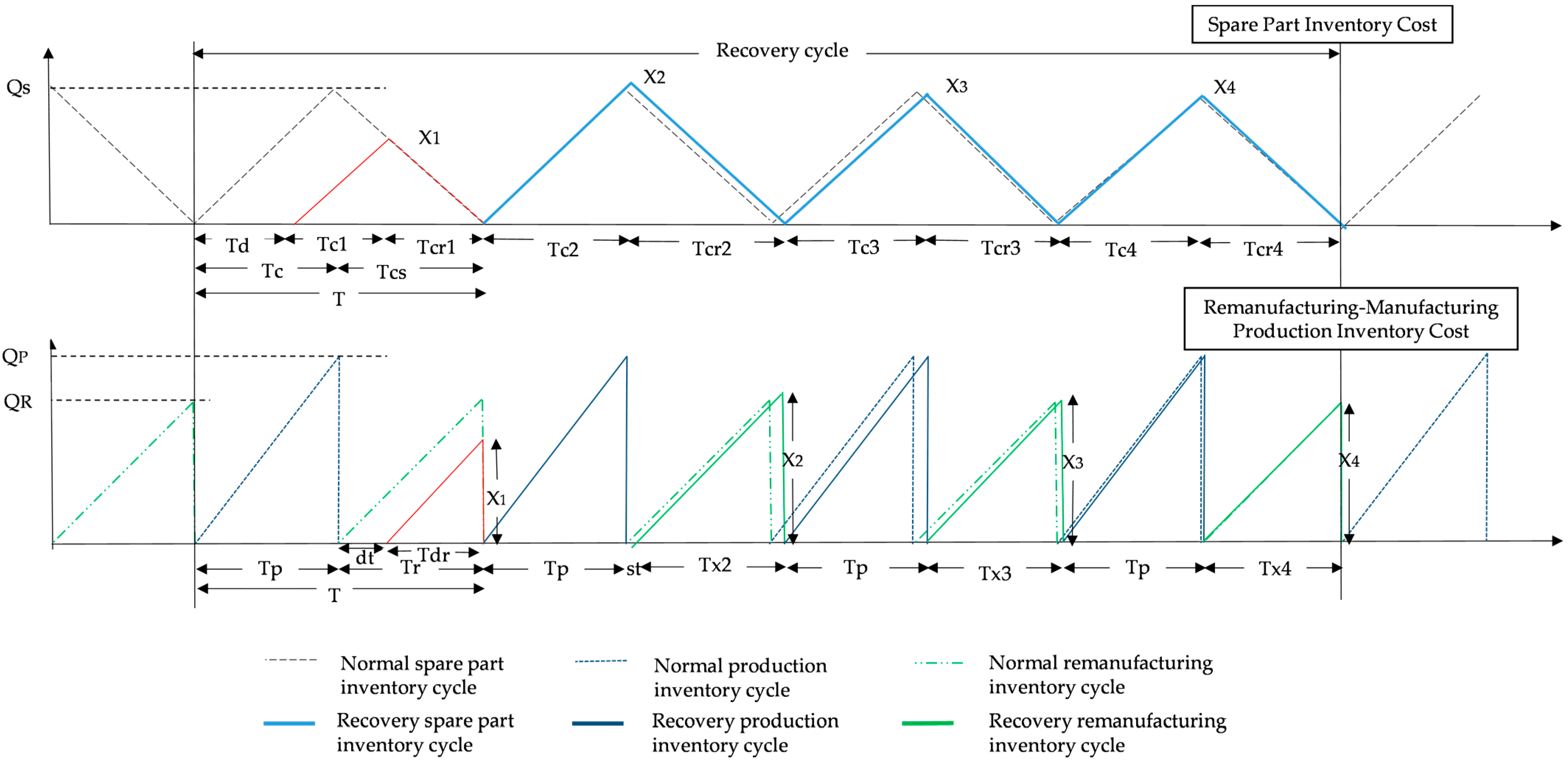
We consider a two-stage production–inventory system that consists of a serviceable inventory (remanufacturing inventory cycle and normal production inventory cycle) and spare parts inventory. The manufacturer alternates two types of production processes, which are a remanufacturing cycle and a normal production cycle, as shown in Figure 1. The serviceable stock is a combination of new products and remanufactured products, which can satisfy market demand. The remanufacturing cycles begin by receiving spare parts from the supplier, which is followed by the production of the remanufactured product, and subsequently the production of new manufactured products. The raw material component for the normal production process uses new components that are different from the remanufacturing process, which uses returned spare parts.

Spare parts collection is disrupted, unable to satisfy the requirements of the remanufacturing process, and disturbs the normal remanufacturing production cycle. The recovery period begins as soon as the disruption occurs. Given that the collection quantity of the spare parts during the disruption is less than the demand of remanufactured production during regular cycles, the production of remanufacturing items is lower than its usual output. This is depicted by the red lines in Figure 1. At this point, some of the customer demand cannot be fulfilled as a result of the disruption and becomes backorders and lost sales. These recovery cycles continue until production returns to a normal schedule and customer demand can be fulfilled within a short time whilst minimising manufacturer loss. For an improved understanding of the problem, we provide the definition of the different terms used in this study as follows:

• Disruption refers to any form of interruption in production.
• Disruption duration is the duration of production interruption.
• Recovery window refers to the duration allocated for recovery (denoted by the vertical black lines), where changes are made to the original schedule. The original schedule is recovered by the end of this duration.
• Recovery plan refers to the new schedule, which includes the optimal quantity of backorders and lost sales in the recovery time window and the optimal number of production cycles required for recovery.
• Backorder is the portion of an order that cannot be delivered at the scheduled time but will be delivered at a later date when available.
• Lost sale refers to when a demand occurs and the item is out of stock and the customer does not wait for the stock to be replenished; hence, the demand is lost.

Disruptions may strike at any moment and anywhere in the production of new manufactured and remanufactured products. It may lead to changes in the behaviour of production flows to the inventory. We assume that disruption occurs in the first remanufacturing cycle, when the arrival of a spare part does not meet the requirement for the remanufacturing process. This study addresses the cost minimisation of recovery cycles so that the manufacturer can prevent a more substantial total loss during disruption. By setting T_d as the disruption period, we assume that the disruption occurs in spare parts collection, before the remanufacturing cycle, consequently disturbing the production cycles of the remanufactured products. Spare parts are collected depending on the demand of the remanufacturing process. Given that the disturbance occurs during spare parts collection, the new quantity of spare parts, S_i, is less than the normal spare parts ordering quantity lot size, Q_s. Then, it affects the quantity production of the remanufactured product, X₁, which is less than the normal remanufacturing production, Q_r. The recovery cycle occurs during the subsequent cycles, and the recovery window duration is defined as the number of recovery cycles, n, where the recovery window ends when the production of the remanufactured and manufactured items return to their original schedule. Although spare part disruption occurs, recovery in the normal manufacturer period (T_p) does not affect the production quantity of newly manufactured products and merely delays its schedule. The production quantity for the newly manufactured products is not disturbed mainly due to its raw material components inventory that includes readily available in stock and is undisrupted; hence, it is not considered in the optimisation model.

2.2. Assumptions and Notations

The following assumptions were used in the development of the recovery model:

• The demand is deterministic.
• The ordering rate of a spare part depends on the demand of the remanufacturing system.
• Disruption occurs when the suppliers cannot provide the requirement of spare parts to the remanufacturing process.
• The production rate of the new product is constant during the recovery period.
• Lost sales and backorders occur during the recovery period.
• During recovery, one recovery cycle is recovery for the remanufacturing and normal production cycles.

The main objective of this study is to develop a mathematical model decision support system for remanufacturing supply chain inventory management considering disruptions. The decision variables include X_i as the remanufacturing quantity for the recovery cycle, T_Xi as the time taken for the remanufacturing cycle in the recovery window and Q_s as the spare part economic ordering lot size.

The following notations are used in the model cost function development:

T: length of production and remanufacturing process cycle (year);

B: unit backorder cost per unit time ($/unit/year);

L: lost sale cost per unit ($/unit);

n: number of recovery cycles in the recovery window.

The following variables denote the serviceable manufacturer’s parameters:

Q_r: remanufacturing lot size in the original schedule (unit);

Q_p: production lot size in the original schedule (unit);

T_r: remanufacturing cycle time (year);

T_s: shortage period when disruption occurs (year);

T_p: normal production cycle time (year);

T_d: disruption period (year);

s_t: production setup time (year);

h_p: holding cost per unit cost of serviceable stock ($/unit/year);

X_i: recovery for remanufacturing lot size in cycle I (i ≥ 1) (unit);

T_Xi: remanufacturing period in recovery cycle i (i ≥ 1) (year);

R: remanufacturing rate (unit/year);

P: normal production rate (unit/year);

A_p: normal production setup cost ($/batch);

A_r: remanufacturing setup cost ($/batch);

B: unit backorder cost per unit time.

The following symbols denote the spare parts manufacturer’s parameters:

Q_s: spare parts ordering lot size (unit);

S_i: spare parts recovery ordering lot size in cycle i (i ≥ 1) (unit);

T_s: spare parts manufacturer ordering cycle time (year);

T_i: spare parts recovery period during a disruption in a cycle i (i ≥ 1) (year);

H_s: holding cost per unit cost of spare parts stock ($/unit/year);

C: spare parts collection rate (unit/year);

D_R: demand rate of spare part use (unit/year).

2.3. Mathematical Formulation

The optimal lot size for Q_p and Q_r and T_p, and T_r for the above ideal system is formulated on the basis of the original work by Mohapatra et al. [44] as follows:

$$Q_p=\sqrt{\frac{2PD{A}_P}{\left(P-D\right)h_p}}$$

(1)

$$Q_r=\sqrt{\frac{2R^{2}C{A}_r}{\left(2R-D\right)\left(R+C\right)h_p}}$$

(2)

$$T_P=\frac{Q_p}{P}$$

(3)

$$T_r=\frac{Q_r}{R}$$

(4)

For this model, we consider four main costs in the recovery cycles. The first one is the set up cost (TC₁), which is rather straightforward as

$$n\left(A_P+A_r\right)$$

(5)

Next, the total cost for inventory holding cost (TC₂) is a derivation of multiplying the unit inventory holding cost by the total inventory during the recovery cycle. Let h_s and h_p represent the holding cost per unit cost of spare parts and the serviceable stock, respectively. The spare part inventory (TC₂₁) is expressed as follows:

$$\begin{gathered} h_s\left[\frac{1}{2}{T}_{c1}{S}_1+\frac{1}{2}{T}_{cr1}{S}_1+\frac{1}{2}{T}_{c2}{S}_2+\frac{1}{2}{T}_{cr2}{S}_2+\frac{1}{2}{T}_{c3}{S}_3+\frac{1}{2}{T}_{cr3}{S}_3+\frac{1}{2}{T}_{c4}{S}_4 \\ +\frac{1}{2}{T}_{cr4}{S}_4+\frac{1}{2}{T}_{c5}{S}_5+\frac{1}{2}{T}_{cr5}{S}_5+\dots \frac{1}{2}{T}_{cn}{S}_n+\frac{1}{2}{T}_{crn}{S}_n\right] \end{gathered}$$

(6)

$$\begin{gathered} =\frac{1}{2}{h}_S\left[\left(T_P+S_{t1}-T_d+T_{X1}\right)S_1+\left(T_{P2}+S_{t2}+T_{X2}\right)S_2+\left(T_{P3}+S_{t3}+T_{X3}\right)S_3\right]+ \\ +\left(T_{P4}+S_{t4}+T_{X4}\right)S_4+\dots \left(T_{Pn}+S_{tn}+T_{Xn)}\right)S_n \end{gathered}$$

$$\begin{gathered} =\frac{1}{2}{h}_S\left[T_P{S}_1+S_{t1}{S}_1+T_{X1}{S}_1+T_{P2}{S}_2+S_{t2}{S}_2+T_{X2}{S}_2+T_{P3}{S}_3+S_{t3}{S}_3 \\ +T_{X3}{S}_3+\dots T_{Pn}{S}_n+S_{tn}{S}_n+T_{Xn}{S}_n-T_d{S}_1\right] \end{gathered}$$

where

$$T_{c1}=T_P+S_{t1}-T_d, T_{cri}=T_{Xi}=\frac{S_i}{C}\mathrm{and}{T}_{ci}=T_P{S}_t\mathrm{when}i>1$$

(7)

Substituting Equation (7) for Equation (6), we obtain

$$T{C}_{21}=\frac{1}{2}{h}_S\left[{\displaystyle \sum }_{i=1}^n\frac{S_i^2}{C}+{\displaystyle \sum }_{i=2}^{n-1}\frac{S_i^2}{Dr}+{\displaystyle \sum }_{i=2}^{n-1}\frac{S{t}_i{S}_i}{Dr}+\left(\frac{S_1}{Dr}-T_d\right)S_1\right]$$

(8)

The holding cost for serviceable inventory (TC₂₂) is expressed as follows:

$$h_p\left[\begin{array}{c}\frac{1}{2}{T}_{X1}{X}_1+\frac{1}{2}{T}_{P1}{Q}_P+\frac{1}{2}{T}_{X2}{X}_2+\frac{1}{2}{T}_{P2}{Q}_P+\frac{1}{2}{T}_{X3}{X}_3\\ +\frac{1}{2}{T}_{P3}{Q}_P+\frac{1}{2}{T}_{X4}{X}_4+\frac{1}{2}{T}_{P4}{Q}_P+\frac{1}{2}{T}_{X5}{X}_5 \end{array}\right]$$

(9)

where

$$T_{Xi}=\frac{X_i}{R}\mathrm{and}{T}_{Pi}=\frac{Q_P}{R}$$

(10)

By inserting Equation (10) into Equation (9), we obtain

$$\frac{1}{2}{h}_p\left[\frac{S_1}{R}{X}_1+\frac{Q_P}{P}{Q}_P+\frac{S_1}{R}{X}_2+\frac{Q_P}{P}{Q}_P+\frac{S_1}{R}{X}_3+\frac{Q_P}{P}{Q}_P+\frac{S_1}{R}{X}_4+\frac{Q_P}{P}{Q}_P+\frac{S_1}{R}{X}_5\right]$$

(11)

Substituting $S_i=X_i$, we obtain

$$T{C}_{22}=\frac{1}{2}{h}_p\left[{\displaystyle \sum }_{i=1}^n\frac{X_i^2}{R}+n\frac{Q_P^2}{P}\right]$$

(12)

The total holding cost can be expressed as

$$T{C}_2=T{C}_{21}+T{C}_{22}$$

(13)

Therefore, by replacing Equations (8) and (12) with Equation (13), the following function for total holding costs is obtained:

$$T{C}_2=\frac{1}{2}{h}_S\left[{\displaystyle \sum }_{i=1}^n\frac{S_i^2}{C}+{\displaystyle \sum }_{i=2}^{n-1}\frac{S_i^2}{Dr}+{\displaystyle \sum }_{i=2}^{n-1}\frac{S{t}_i{S}_i}{Dr}+\left(\frac{S_1}{Dr}-T_d\right)S_1\right]+\frac{1}{2}{h}_p\left[{\displaystyle \sum }_{i=1}^n\frac{X_i^2}{R}+n\frac{Q_P^2}{P}\right]$$

(14)

Next is the total backorder cost (TC₃) formulation, which is the product of the unit backorder cost, B, with the backorder quantity of each cycle, Xi, and delay time, Delay_i, adapted from [45]. The formulation can be derived as follows:

$$B\left({\displaystyle \sum }_{i=1}^n{X}_i. Dela{y}_i\right)$$

(15)

Delay_i is derived for each cycle. Delay_n is the time delay for the cycle, n. Therefore, the total Delay_i can be expressed as

$$Dela{y}_i={\displaystyle \sum }_{i=1}^n\left[T_{xi}+st\right]-n{T}_r$$

(16)

By substituting Equation (15) for Equation (14), the backorder cost (TC₃) becomes

$$B\left[{\displaystyle \sum }_{i=1}^n{X}_i . \left({\displaystyle \sum }_{i=1}^n\left[T_{xi}+st\right]-n{T}_r\right) \right]$$

(17)

Lastly, the total lost sale cost (TC₄) is expressed as

$$L\left(n{Q}_R-{\displaystyle \sum }_{i=1}^n{X}_i\right)$$

(18)

Adding the cost component expressions above gives the overall total cost of recovery for the entire system, TC. Therefore, the mathematical model is a cost minimisation problem and is presented as follows:

$$\begin{array}{c}Min TC=T{C}_1+T{C}_2+T{C}_3+T{C}_4\hfill \\ =n\left(Am+Ar\right)+\frac{h_s}{2}\left[{\displaystyle \sum }_{i=1}^n\frac{S_i^2}{C}+{\displaystyle \sum }_{i=2}^{n-1}\frac{S_i^2}{Dr}+{\displaystyle \sum }_{i=2}^{n-1}\frac{S{t}_i{S}_i}{Dr}+\left(\frac{S_1}{Dr}-T_d\right)S_1\right]+\frac{h_p}{2}[{\displaystyle \sum }_{i=1}^n\frac{X_i^2}{R}+\hfill \\ n\frac{Q_P^2}{P}]+B\left[{\displaystyle \sum }_{i=1}^n{X}_i . \left({\displaystyle \sum }_{i=1}^n\left[T_{xi}+st\right]-n{T}_r\right) \right]+L\left(n{Q}_R-{\displaystyle \sum }_{i=1}^n{X}_i\right)\end{array}$$

(19)

Subject to the following constraints

$$X_1\le Q_R$$

(20)

$$S_1\le Q_S$$

(21)

$${\displaystyle \sum }_{i=1}^n{X}_i\le nTR – {\displaystyle \sum }_{i=1}^{n}S{t}_i – T_d$$

(22)

$${\displaystyle \sum }_{i=1}^n{X}_i+n{Q}_P\ge n\left(Q_P+Q_R\right)$$

(23)

all decision variables are nonnegative.

Objective function (19), which is used to minimise TC, considers the setup cost, holding cost, backorder cost and lost sale cost. Equations (20) and (21) certify that the production of remanufacturing during the recovery schedule does not exceed regular remanufacturing production due to disruption in spare parts collection. Equation (22) ensures that demand is fulfilled within a period, whereas Equation (23) is a serviceable production capacity constraint. All decision variables must be in positive values. By solving the developed model for X_i, S_i and n, an optimal recovery plan with a minimal TC can be obtained even for systems under disruption.

3. Numerical Analysis

Various experiments are discussed in this section, demonstrating the applicability and efficiency of the proposed model and method. The mathematical model presented in this study was categorised as a nonlinear constrained quadratic programming problem and was solved using the branch and bound algorithm.

The basic parameters used in this model or benchmark parameter were defined as test problem 1, as tabulated in

Table 2. Set of tests with different datasets.

Parameters	Test 1	Test 2	Test 3	Test 4	Test 5
Ap	200	200	200	200	200
Ar	250	300	250	250	250
hp	22	22	44	22	22
hs	18	18	18	36	18
B	25	25	25	25	25
L	50	50	50	50	50
Td	0.02	0.02	0.02	0.02	0.04

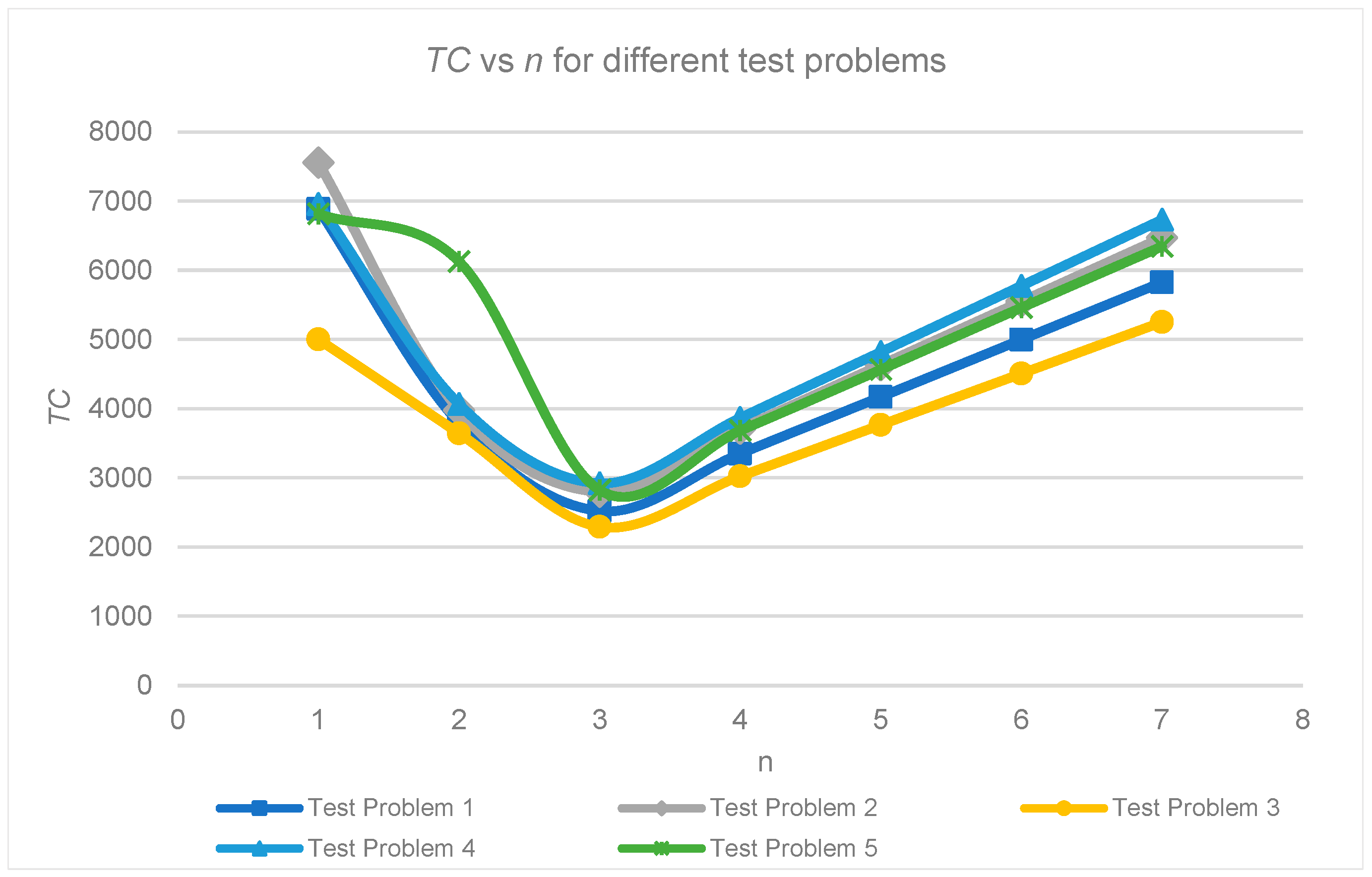
. The holding cost value, h_p and h_s, and the rate for production, remanufacturing and demand, P, R and D_R, respectively, were adapted from [46], whereas the disruption parameters were based on the data deemed suitable for the developed model from [45]. The developed model was then tested with five sets of parameters to ensure that valid and credible output was generated. In

Table 3. Results for the test with different datasets.

n	Test 1	Test 2	Test 3	Test 4	Test 5
1	6887.58	7558.72	5003.73	6958.46	6816.13
2	3793.30	3978.42	3645.81	4065.64	6127.67
3	2522.31	2799.95	2922.9	2922.9	2822.09
4	3351.32	3712.84	3023.8	3867.74	3681.98
5	4171.71	4618.49	3765.05	4820.86	4564.9
6	4997.84	5551.58	4508.54	5776.05	5459.32
7	5825.42	6472.24	5252.92	6732.06	6347.98

, test problem 2 provides the pattern behaviour of the remanufacturing setup cost when increased. For test problems 3 and 4, the holding cost for the serviceable stock and spare parts were doubled, respectively. The disruption time was also doubled to 0.04 s in test problem 5 to show the effect of an increased disruption time to the optimal solution. The results are graphically illustrated in Figure 2, showing the optimal solution for each test problem lies at n = 3, where the minimum total costs are obtained. The plot in Figure 2 shows consistent convex curves, implying that the model and solution procedure established in this study provides global optimal solutions [47].

4. Sensitivity Analysis

In this section, a sensitivity analysis is conducted to analyse the impact of system efficiency on analysing the optimal TC values with various datasets. To perform the sensitivity analysis, we run the same experiment with precisely the same parameters and characteristics but with a different setup cost, unit inventory holding cost, backorder cost, lost sale cost and disruption time. All the other parameters, if not varied, remain unchanged based on the dataset for test problem 1.

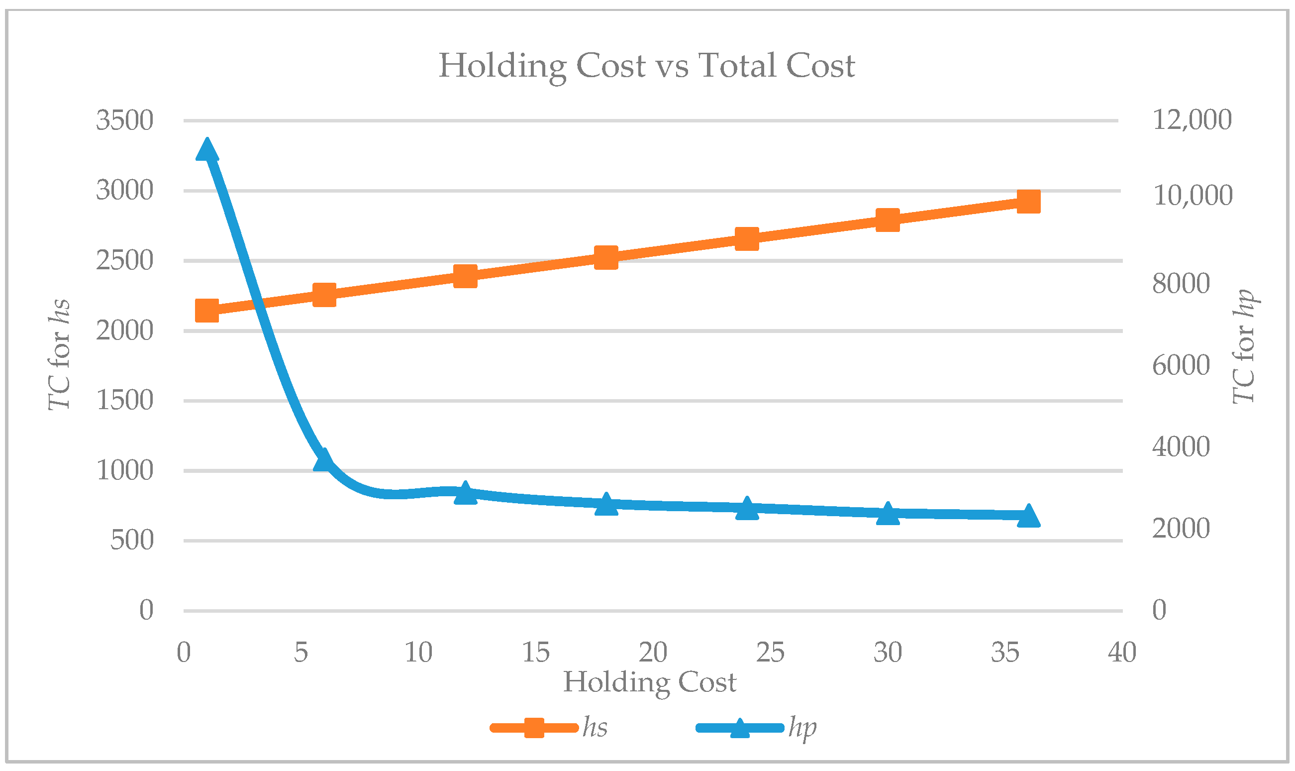
The setup cost for remanufacturing and production was increased from 50 to 350 and was tested using the test problem dataset, as shown in Figure 3. The plotted graph shows that TC is directly proportional to the production and remanufacturing setup costs. Given that the setup cost is one of the components considered in the developed model, increments in setup cost increase the overall TC. The unit inventory holding cost in the mathematical model is the holding cost for serviceable and spare parts stock. Figure 4 displays the results of TC with the increment in the unit inventory holding cost when using test problem 1 parameters. The other parameters remain unchanged except for the total holding cost value for the serviceable and spare parts stock. The results of this test reveal that when h_s is increased, the total cost also increases. However, the increment in hp drops the TC value due to the relationships between Q_r, Q_p and h_p based on Equations (1) and (2). The value for Q_r and Q_p act inversely proportional to the h_p value. As h_p increases, Q_r and Q_p decrease, as does TC.

Figure 5 depicts the results derived from the tests conducted for the relationship between the backorder unit cost and the backorder cost, TC and n. The plotted graph shows that the backorder cost increases as the backorder unit cost increases. Similarly, the TC behaviour increases when the backorder unit rises. However, the optimal number of cycles decreases from n = 3 to n = 2 as the backorder unit cost increases. This decrease occurs due to the increment of the backorder, which is less cost effective than lost sales during the recovery schedule. Hence, the lost sale cost affects the overall TC, and the unmet demand becomes lost sales. At the same time, the quantity production of the serviceable item is reduced, reducing recovery time.

The effect of changing T_d on TC and n is depicted in Figure 6. One can argue that TC depends on the changes in T_d. The minimum value of TC decreases at n = 3 until T_d reaches 0.045. Conversely, TC sharply increases at 5% after T_d is more than 0.045 and TC achieves a maximum value when n = 2. Thus, as T_d increases, the affected remanufacturing cycle’s quantity is less than its regular schedule, and the unfulfilled quantity of demand escalates, thus influencing the lost sales cost, resulting in additional costs to the TC. Hence, the recovery method is optimal only until a certain T_d, after which a backup supplier might be a better option. Alternative recovery options must be determined for the manufacturer to overcome additional TC and further reduce company loss.

5. Case Study

After various tests were conducted on the developed model, a real case study was performed to validate the mathematical model. Amongst the advantages of real case studies is being able to explain the complexity of real situations that may not be obtained through simulations, experiments or surveys by detailing data in a real-life environment [48]. Therefore, data from selected industries were obtained to implement the actual case study method. The selected company, Company A, has agreed to allow the shared data to be used in this study.

5.1. Company Overview

Company A provides repair services for heavy machinery vehicles and its components, especially prime movers. According to the records provided, more than 30 prime movers all over Malaysia’s east coast avail of repair services from this company. The repair cases conducted in this company are specifically related to the engine, brake, lubrication and transmission systems.

For the actual case study for the development of this model, the transmission system was chosen because according to an interview with the company, the percentage of obtaining spare parts during the overhaul of the transmission system is high. For this reason, the study on transmission system spare parts is explained in more detail in the next subsection.

The developed model mainly aims to reduce the cost of recovery that companies have to bear when disruptions occur. The most considerable disruption experienced by most companies in the past years was related to the COVID-19 pandemic [48]. The first case in Malaysia was detected in January 2020, and COVID-19 cases became more contagious. Following the sudden increase in cases, the government decided to implement a movement control order (MCO) in March 2020. Consequently, the Malaysian economy suffered a severe collapse and affected the income of most sectors.

Company A was also affected when the MCO was implemented throughout Malaysia. The highest repair frequency in the company is the brake system, which is followed by the lubrication system and the transmission system. However, spare parts for the brake system are readily available, and the company does not face difficulties in the process of overhauling the brake system.

The data provided are related to the replacement process of the clutch component in the transmission system, which is the Clutch Servo Pump. These components are supplied by the main spare parts supplier, Supplier V, located in Kuala Lumpur, Federal Territory.

5.2. Model Validation and Discussion

The study on the transmission system spare parts was conducted by using the data obtained from the industry, as depicted in

Table 4. Data obtained from the industry during a disruption occurrence.

Parameter	Value
Ap	520
Ar	650
hp	46.8
hs	57.2
B	700
L	1000
Td	0.008
D	2600
R	5200
C	5460
P	7800

, which is for the case when a disruption occurred.

LINGO 15.0 software was used to solve the model with the case study data. LINGO serves as a simple and affordable instrument for solving linear and nonlinear optimisation problems; it can formulate complex problems, resolve them and analyse the outcomes. Compared with other modelling packages, LINGO includes a set of built-in solvers that are directly linked to the modelling environment, which makes it convenient to tackle a wide variety of problems [49]. Other comparable optimisation software are available in the market, but they come with several disadvantages. For instance, CPLEX and MATLAB Optimisation Toolbox are powerful solvers; however, both are complex to use effectively and lack user-friendliness, particularly for those who are less fluent with programming languages. Microsoft Excel solver is another widely used alternative but has a limitation in the problem size which makes it not suitable for large-scale or complex optimisation problems. LINGO software is favoured because it is a complete tool with rich language to clarify the optimisation model and solve it efficiently [50] with fast solvers [51].

The developed model was solved by utilising the data in Table 4, and the optimal TC results were identified, as shown in

Table 5. Actual total cost values for the case study.

n	TC1	TC2	TC3	TC4	TC
1	1170.00	622.45	0	41,600.00	43,392.45
2	2340.00	1471.98	2136.48	10,944.07	16,892.53
3	3510.00	2299.86	6168.66	3936.10	15,914.62
4	4680.00	3443.29	13,450.64	0	21,573.94
5	5850.00	4389.72	20,527.84	0	30,767.56
6	7020.00	5455.82	28,608.70	0	41,084.52
7	8190.00	6678.45	37,319.96	0	52,188.41

. As the recovery cycle increases, the optimal total cost TC also increases due to increased setup costs, although the optimal TC value occurred at n = 3 (TC = 15,914.62) due to the trade-off between the cost of backorders, TC₃, and the cost of lost sales, TC₄. The TC calculation in the table below is for a specific period only. However, if this disruption continues, it could affect the company’s annual income.

The company takes effective mitigation measures to reduce the negative impact, especially on the company’s finances from bankruptcy. Amongst the measures taken by this company is to obtain spare parts supply from backup suppliers or second suppliers. Based on the interviews, the company stated that the costs the company had to bear may exceed the annual budget for production costs, but it was enough to sustain the company’s business operations.

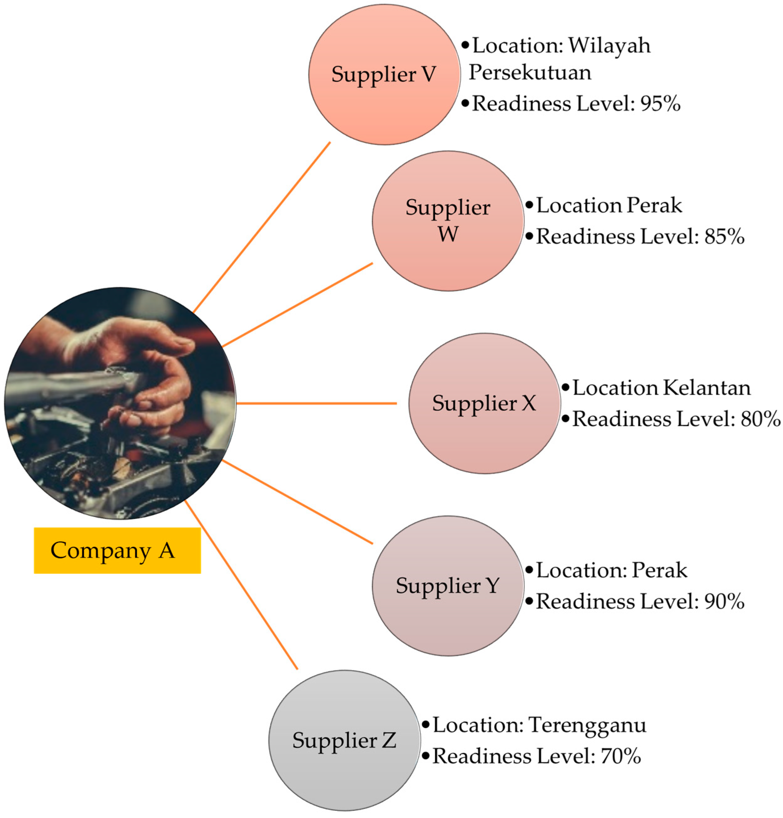
The company has several backup suppliers who may be able to supply their spare parts requirements, consisting of Supplier W (Perak), Supplier X (Kelantan), Supplier Y (Perak) and Supplier Z (Terengganu). The selection to obtain spare parts is based on the cost per unit of spare parts and the length of time taken by the supplier to provide the spare parts as requested. In addition, the level of availability of spare parts is crucial for manufacturers in planning the company’s production strategy. Figure 7 shows the selection factors between suppliers in the decision to obtain spare parts from the suppliers that have been mentioned. Location is also an important factor in the selection of spare parts suppliers because location selection may remarkably reduce delivery or purchase time and subsequently reduce the risk of disruption.

Nevertheless, the level of readiness or availability also plays a vital role in the selection of suppliers. The higher the percentage of spare parts availability, the more attractive it is for the manufacturer to obtain supplies from suppliers. For example, Supplier Z is the supplier that has the least distance from Company A, but the level of availability of spare parts is the lowest; it is possible that the required spare parts are unavailable, a longer period may be needed to fulfil the order, or the parts may be sold at a higher price. This case is common when customers do not have much choice and are in desperate need of spare parts.

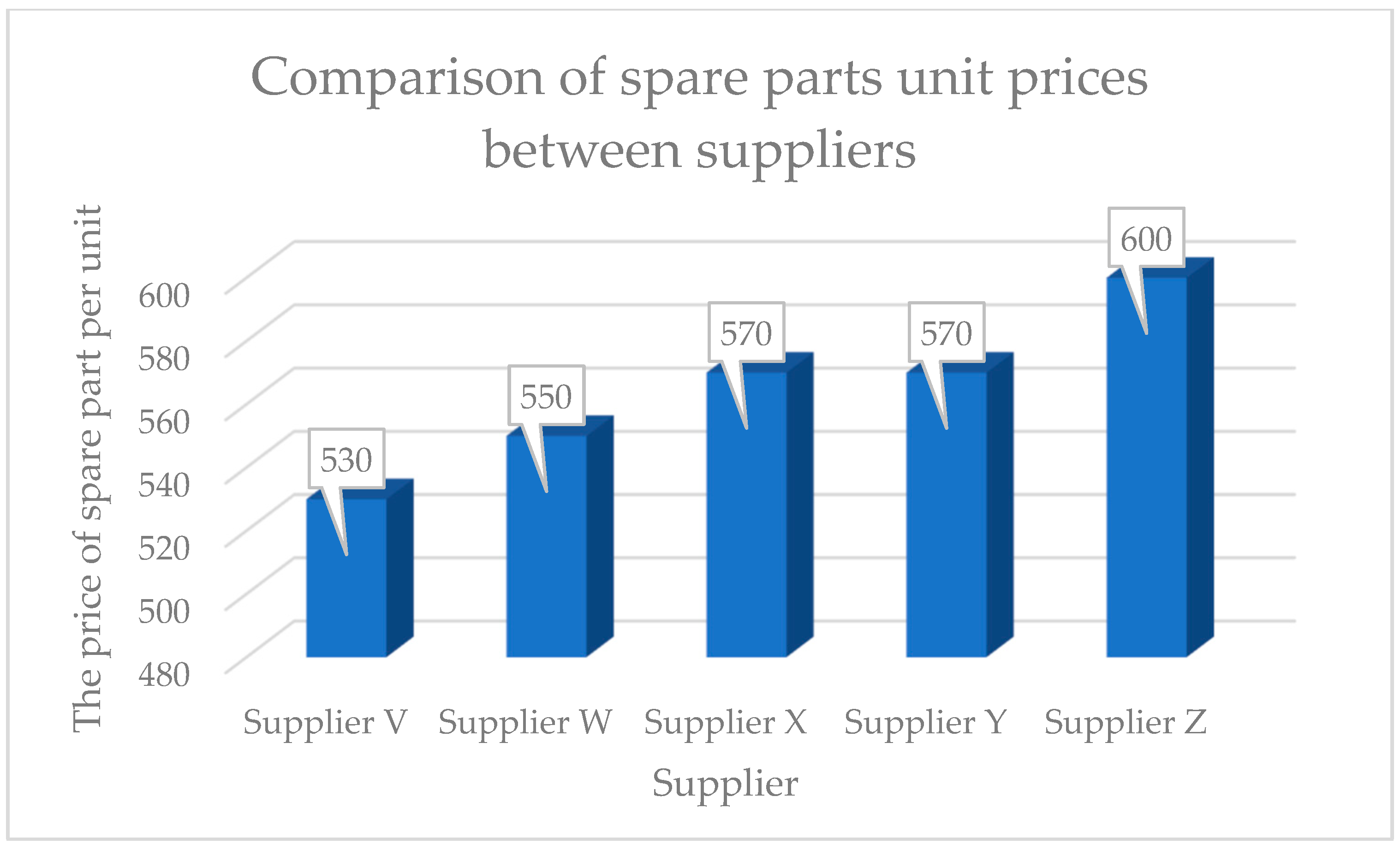
Figure 8 shows a comparison of unit prices for spare parts between suppliers. Supplier V offers the lowest price per unit of spare parts compared with the other suppliers. Supplier Z recorded the highest price even though it was the closest to Company A. This high price is due to the limited number of spare parts suppliers around the area, which in turn gives these suppliers the opportunity to raise prices. Although Supplier W has a high percentage of spare parts provision, the supply of spare parts for the Clutch Servo Pump could not be fulfilled due to internal problems faced by the company, causing the preparation period to be considerably long despite the low and attractive price offered.

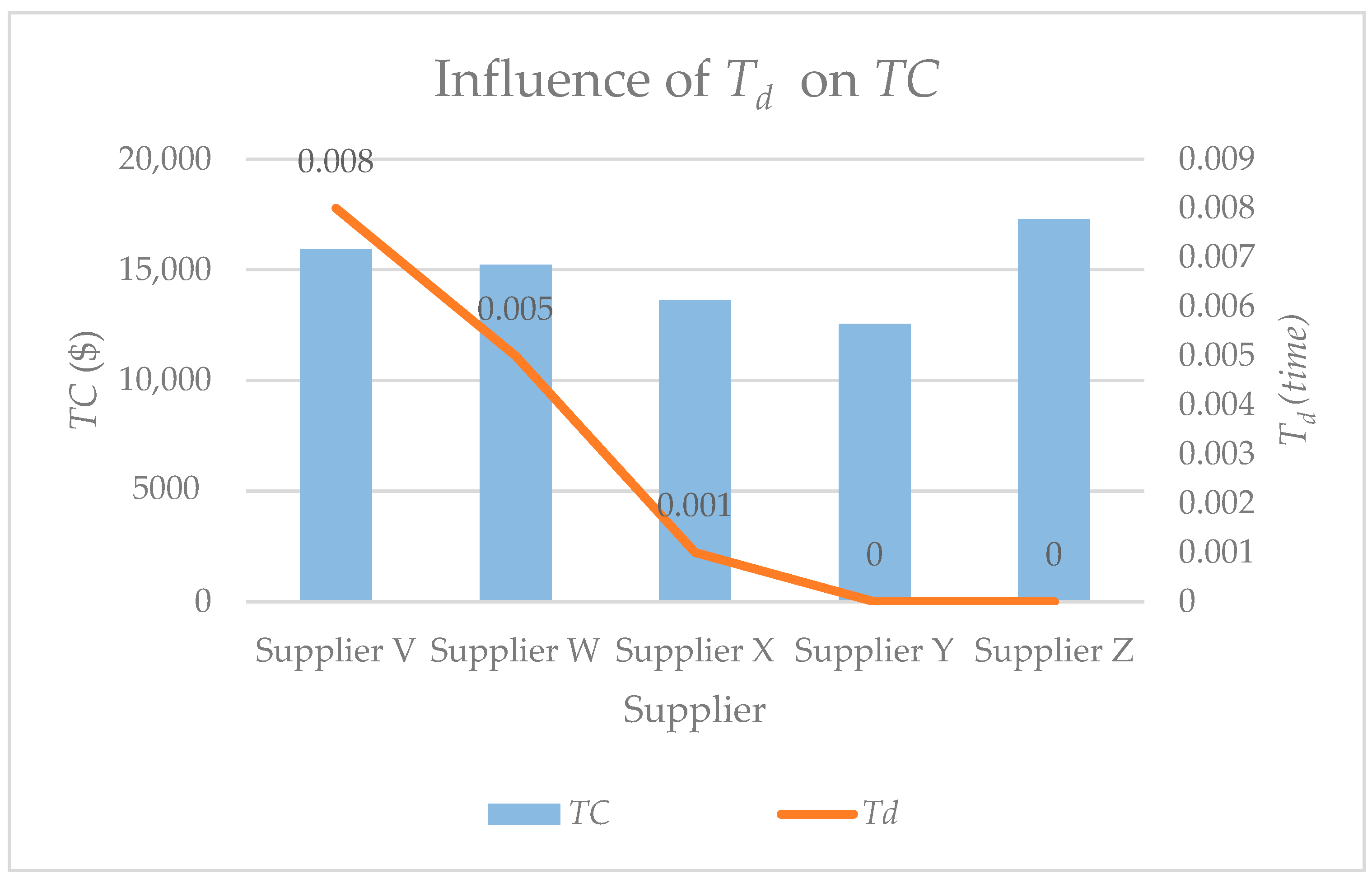
The comparison between the spare parts disruption period and TC is further elaborated in Figure 9. During the disruption, Supplier Y recorded the lowest TC value amongst the other suppliers. Although the unit price of RM 570 is equal to the unit price of spare parts from Supplier X, the disruption period, T_d, for Supplier X is higher (0.001), thus affecting the overall TC to repair the transmission system. As observed from the behaviour of the line graph that shows the preparation period by each supplier during the disruption, Supplier Y and Supplier Z can supply spare parts directly to Company A, but the difference in cost per unit causes a gap between the total recovery cost (TC) for these two suppliers, where Supplier Y becomes more preferable due to the lower cost offered in addition to the zero disruption time.

In conclusion, several factors, such as the price per unit cost of spare parts, disruption period and total recovery costs, influence the manufacturer’s decision to make the right choice in dealing with the disruption event. We recommended that the management analyse the entire total costs involved during the disruption and its impact on the company’s economy either for the current period or for the long run. The management may also evaluate the characteristics of a quality backup supplier by evaluating the current issues faced by the management, considering the optimal total costs as suggested by the model by evaluating the different cost component allocations from the supplier.

6. Managerial Implications

This study analyses the impact of parts supply disruptions on the remanufacturing industry. The management may take several mitigation measures to reduce the negative impact on the company, especially in terms of the company’s economy and reputation. The disclosure of the cost components involved in the calculation of total recovery costs can provide an early insight to the management in terms of dealing with issues related to the company’s expenses in the event of disruptions. To reduce recovery costs, backup suppliers can be considered to reduce the manufacturing period and meet customer demand in a timely manner. Moreover, the management must know the economic status of their supply chain system to reduce the negative implications of the company in the long run.

Amongst other mitigation measures that can be implemented by the management is to obtain the supply of spare parts from different suppliers by comparing the price per unit of spare parts components, the level of availability and the time period for them to be obtained. In addition, incorporating optimisation methods is essential for decision making in the remanufacturing sector; these methods can help managers make decisions when faced with various process complexities and uncertainties [52]. Utilising optimisation techniques, such as the developed model, can further aid manufacturers in determining the effects of disruption for longer periods, particularly when selecting backup suppliers during disruptions.

7. Conclusions

This study presents a mathematical model that determines the recovery schedule for the remanufacturing production system after the spare parts collection cycle is disrupted. Intending to minimise TC, we assume that only the remanufactured quantity is affected after disruption, whereas the quantity for the normal manufactured item remains constant. The solution of the developed model not only minimises the overall TC but also helps to optimise the quantity for each remanufacturing cycle during the recovery schedule such that recovery duration is minimised. The model was solved as a nonlinear quadratic programming problem using the branch-and-bound algorithm.

From the numerical experiment performed, test runs of five different problems demonstrate that the model gives good optimal solutions, as observed from the convex curves generated from the plotted solution points. The results from the sensitivity analysis show that parameters, such as the remanufacturing holding cost, lost sale cost and backorder unit cost, have a considerable influence on the model’s total recovery cost. The disruption time parameter is also remarkable in contributing to the change in the optimal TC. The pattern of the solution for the serviceable item production relies remarkably on the disruption period in the normal cycle. As the disruption time increases, the portion of unmet demand during the disruption cycle also rises. This behaviour contributes to the pattern of lost sales and backorder quantities to achieve the minimal TC, in which the developed model identifies the optimal quantity of shortages that become either lost sales or backorders, depending on the system’s recovery schedule.

Furthermore, the results from the conducted case study imply that the manufacturer’s choice in handling a disruption event is influenced by various factors, including the cost per unit of spare parts, the duration of disruption and the overall recovery costs. Back-up supplier selection is not merely dependent on the cost per unit of spare parts but also relies on the supplier’s preparation time and readiness level. Hence, utilising the developed optimisation model enables remanufacturers to capture these important aspects during the decision-making process and ultimately minimise the cost of unexpected disruptions to their business. For an explanation of the nomenclature used in this study, please refer to

Table 6. Nomenclature used in this study.

Abbreviation	Definition
EoL	End-of-life
EoQ	Economic order quantity
JIT	Just-in-time
CLSC	Closed loop supply chain
TC	Total cost
TC1	Setup cost
TC2	Total holding cost
TC3	Total backorder cost
TC4	Total lost sales cost
TC21	Holding cost for spare parts inventory
TC22	Holding cost for serviceable inventory

.

This work can be expanded through the integration of certain factors. Future work may consider several recovery processes (e.g., recyclable, repairable and refurbished) or a stochastic system for the recovery processes. Furthermore, future studies may investigate other environmental factors, such as carbon dioxide emission and energy usage, such that sustainability goals in the remanufacturing industry could be improved more comprehensively.