Design a Robust Proportional-Derivative Gain-Scheduling Control for a Magnetic Levitation System

Abstract

This study focuses on the design of a robust PD gain-scheduling controller (PD-GS-C) for an unstable SISO (single-input, single-output) magnetic levitation system with two electromagnets (MLS2EM). Magnetic levitation systems offer various advantages, including friction-free, reliable, fast, and cost-effective operations. However, due to their unstable and highly nonlinear nature, these systems require sophisticated feedback control techniques to ensure optimal performance and functionality. To address these challenges, in this study, we derive the nonlinear state-space mathematical model of the MLS2EM and linearize it around five different operating points. The PD-GS-C controller aims to stabilize the system and improve steady-state control error. The strategy for obtaining the PD controller gains involves a parameter space technique, which specifies performance requirements. This technique results in ranges of proportional ($K_P$) and derivative ($K_D$) gains that are used by the PD-GS-C structure. To optimize the controller’s performance further, we utilize the big bang–big crunch optimization technique (BB-BC) to determine the optimal PD gains within the specified ranges. The optimization process focuses on achieving optimal performance in terms of a specific performance index function. This function quantifies the system’s time-domain step response criteria, which include minimizing overshoot percentage, settling time, and rising time. The index function is inversely proportional to the desired performance criteria, meaning that the goal is to maximize the index function to optimize the system’s performance. To validate the effectiveness and viability of the proposed strategy, we conducts MATLAB simulations and real-time experiments. The simulations and experimental findings serve to demonstrate the controller’s performance and verify its capabilities in stabilizing the MLS2EM magnetic levitation system.

1. Introduction

A magnetically levitated mechanism (MAGLEV), also called magnetic suspension, is a naturally occurring phenomenon whereby an antigravity ferromagnetic item is maintained without any other sources except an electromagnetic field with no interaction with the external field [1]. Considering the sophistication of electromagnetic theory, this phenomenon has a broad range of applications, such as high-speed trains, frictionless melting, and magnetic bearings. With the rapid advancement of electronics and advanced control theory, magnetic levitation can be applied for a variety of practical purposes [2]. MAGLEV is a nonlinear, open-loop, unstable system that is challenging to model and control. Magnetic levitation systems are controlled as SISO system architectures, and just one electromagnet in the simplest and most common arrangement [3]. Such systems (MLS1EM) utilize magnetic forces created by providing the electromagnet and one-axis distance sensor with the necessary voltage [4]. In more complex arrangements (MLS2EM), a secondary electromagnet can be used to produce an external gravitational pull that is distinct from that produced by the first [5].

For magnetic levitation systems, various well-known linear and nonlinear control techniques have been developed. Highly nonlinear operating differential equations make nonlinear controllers more desirable. To provide excellent productivity, many nonlinear control schemes require precise understanding of nonlinear plant effects. Practical implementations of nonlinear controllers are made challenging by the modeling of uncertain parameters in the MAGLEV model. On the other hand, the approximating linear model obtained by adjusting the system behavior around a preferred operating point is used in linear controller design, and as a result, the controllers are typically valid around the operating point. Linear controller performance is enhanced by using a gain-scheduling process to accommodate different operating points and enlarge the operating region [6].

Numerous efforts have recently been published in the literature to control magnetic levitation systems. Input–output and input-state linearization approaches are among the feedback linearization-based controllers that have been developed [7,8,9,10,11,12], in addition to the design of linear state feedback controls [13], observer-based controls [14,15], cognitive strategies [16,17,18], slide mode control [19,20,21], backstepping control [22], model-based predictive control (MPC) [23,24], adaptive H-infinity tracking control [25], and proportional–integral–derivative (PID) control [4,26]. In addition, there are several adaptive control schemes that have already been presented in the past few years for positioning control schemes and magnetic levitation technologies. Some of these constructions can be found in [27,28,29,30,31,32,33,34,35]. An interesting method to consider for magnetic levitation positioning is that of finite time control, such as those mentioned in [36].

Gain-scheduling controlled systems are common in today’s adaptive control applications, and they are succinctly examined as follows. Slide mode control and fuzzy-based gain scheduling of exact feed-forward linearization control for a magnetic levitation system are described in [37]. The authors in [38] discusse a high-gain adaptive output feedback control for a maglev apparatus. Using a Smith predictor, The authors of [39] provided a proportional–integral–derivative (PID) gain-scheduling control with second-order linear parameter variation, which eliminates time-varying delay. Additional intriguing adaptive gain-scheduling control mechanisms for practical, applications are discussed in [40,41,42,43,44]. The authors of [45] presented the design of a proportional–integral gain-scheduling control for position control of a sphere in a laboratory magnetic levitation system. The unstable and nonlinear mathematical model of the process is linearized at seven operating points. The authors of [46] presented a gain-scheduling control design procedure for classical proportional–integral–derivative controllers (PID-GS-C) for a positioning system. The method was applied to a laboratory magnetic levitation system with two electromagnets (MLS2EM), which allowed for several experimental verifications of the proposed solution.

The authors of [47] provided a coherent approach to the tuning of PID controllers. By using the model-reference robust tuning (MoReRT) method, the authors proposed a way to achieve robust and effective PID controller tuning. The authors in [48] delved into deterministic multiobjective optimization methods, which are used to solve control system design problems that involve multiple conflicting objectives. The authors developed algorithms for two-degree-of-freedom PID control. An optimal indirect internal model control-proportional derivative (iIMC-PD) controller was designed as a two-loop control structure to regulate the dynamics of integrating processes with dead time [49]. The authors in [50,51] focused on analyzing optimal controller settings for controllers with a proportional–integral–derivative (PID) structure. Analysis was conducted by considering two key factors: the operating mode of the control loop (either servo or regulation mode) and the tuning mode of the controller. The goal was to determine controller settings that lead to optimal performance based on the specific operating and tuning modes.

The position control of a ferromagnetic sphere in a laboratory magnetic levitation system with two electromagnets (MLS2EM) is the topic of this research. The control input is provided only to the upper electromagnet, and the bottom electromagnet can be subjected to the generated external disturbance. Two control architectures are developed to stabilize the system: proportional-derivative control (PD-C) and proportional-derivative gain-scheduling control (PD-GS-C). To enable the use of straightforward control techniques, the given mathematical model of the MLS2EM nonlinear system is linearized around five operating points. This linearization simplifies the control design process by allowing for the application of conventional control methods. For the PD-C controller, a parameter space technique is employed to design five robust PD controllers. The goal is to guarantee system stabilization and improve the steady-state control error. The parameter space approach provides ranges of proportional ($K_P$) and derivative ($K_D$) gains, which are crucial for the PD-GS-C structure. In the PD-GS-C architecture, the control gains are adaptively adjusted to match changes in the operating points. This adaptability is important because the bottom electromagnet of the MLS2EM system may be subjected to external disturbances, which could affect the system’s behavior and performance. To optimize the PD-GS-C controller’s performance, we use the big bang–big crunch optimization technique (BB-BC) to determine the optimal PD gains within the specified ranges obtained by the parameter space approach. The goal of optimization is to achieve the best possible performance for MLS2EM magnetic levitation. Finally, this research aims to demonstrate effective position control for a ferromagnetic sphere in an MLS2EM system using both PD-C and PD-GS-C controllers. By considering external disturbances and adapting the control gains to changing operating conditions, the proposed control architectures seek to stabilize the system and ensure accurate positioning of the ferromagnetic sphere. The use of linearization, parameter space techniques, and optimization methods contributes to the achievement of robust and efficient control of an MLS2EM magnetic levitation system.

The structure of this article is described as follows. Potential models for the MAGLEV system are described in Section 2, including an explanation of the physical principles of magnetic levitation and how the system can be mathematically modeled. The parameter space approach, which sets the boundaries for the stabilization of PD gains, is described in Section 3. The utilization of the big bang–big crunch optimization technique (BB-BC) to obtain an optimal set of PD gains is also discussed in the same section. The PD gain-scheduling control (PD-GS-C) is presented in detail in Section 4, and the concept and architecture of the controller are explained. Section 5 contains illustrations and discussions of the experimental outcomes obtained through simulations, including graphs and charts that showcase the performance of the proposed PD-GS-C controller in the magnetic levitation system. Finally, Section 6 presents the key observations and findings of this research; we summarize the achievements of the study, discuss the effectiveness of the proposed PD-GS-C controller, and highlight any potential areas for further improvement or research.

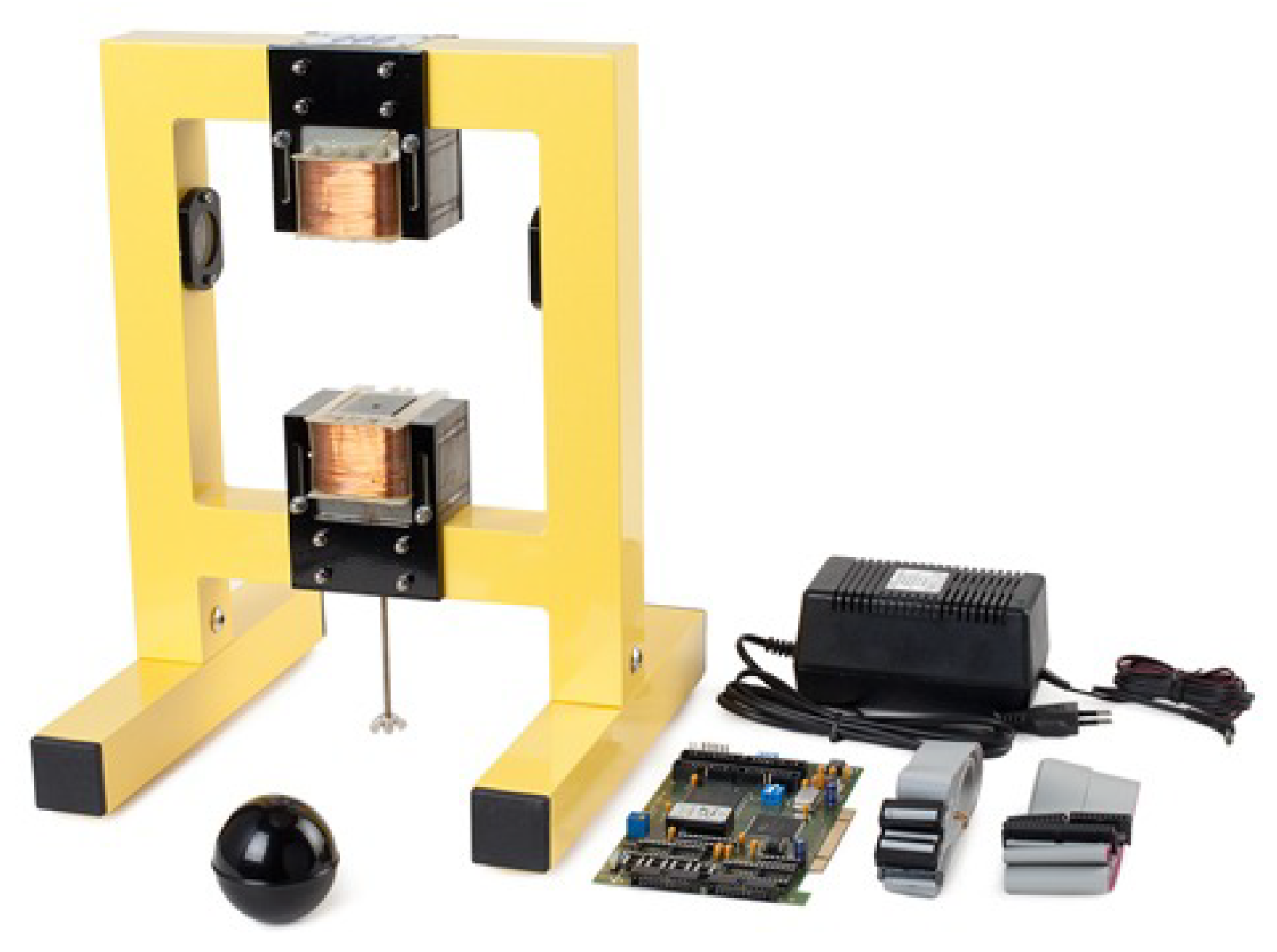
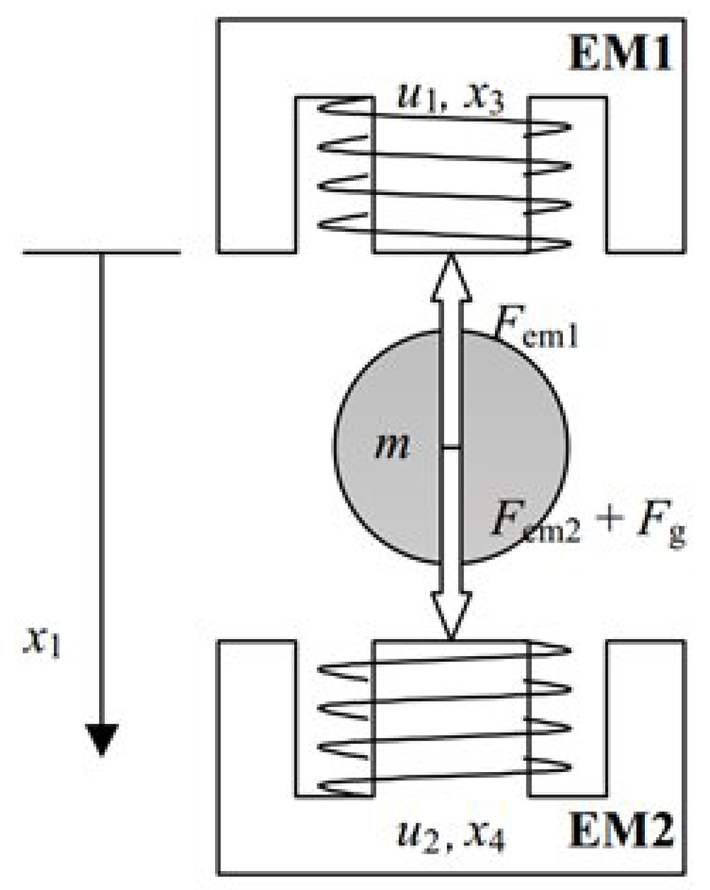
2. Magnetic Levitation and Modeling

Figure 1 illustrates the ML2SEM magnetic levitation equipment, which serves as an experimental benchmark for the theoretical validation of the magnetic levitation principle by suspending a ball of steel in the air while applying magnetic force. Due to its significant nonlinearity, this system is suited for use in university laboratories and is safe for assessment of the effectiveness of various controller types [52].

A schematic diagram of the ML2SEM-controlled plant is shown in Figure 2, where EM1 and EM2 are the top and bottom electromagnets, respectively; m is the sphere’s mass; $F_{em1}$ and $F_{em2}$ are the electromagnetic forces; and $F_g$ is the force of gravity [52].

The state-space mathematical model of the ML2SEM’s is expressed as:

$$\begin{array}{c}\dot{x_1}=x_2\hfill \\ \dot{x_2}=-\frac{F_{em1(x_1,x_3)}}{m}+g+\frac{F_{em2(x_1,x_4)}}{m}\hfill \\ \dot{x_3}=\frac{1}{f_i\left(x_1\right)}(k_i{u}_1+c_i-x_3)\hfill \\ \dot{x_3}=\frac{1}{f_i(x_d-x_1)}(k_i{u}_2+c_i-x_4)\hfill \end{array}$$

(1)

The nonlinear functions in Equation (1) can be described as follows.

$$\begin{array}{c}{F}_{em1}(x_1,x_3)=x_3^2\frac{F_{emp1}}{F_{emp2}}exp(-\frac{x_1}{F_{emp2}})\hfill \\ F_{em2}(x_1,x_4)=x_4^2\frac{F_{emp1}}{F_{emp2}}exp(-\frac{d-x_1}{F_{emp2}})\hfill \\ f_i\left(x_1\right)=\frac{f_{ip1}}{f_{ip2}}exp(-\frac{-x_1}{f_{ip2}})\hfill \end{array}$$

(2)

where, $x_1\in [0,0.016m]$ is the sphere position, $x_2\in \Re$ is the speed of the sphere, and $x_3\mathrm{and}{x}_4\in [0.03884,2.38]$ are the currents in the electromagnetic coil in amperes. The control signals that are applied to EM1 and EM2 are $u_1\mathrm{and}{u}_2\in [0.00498,1]$, respectively; d denotes the spacing between electromagnets minus the diameter of the ball; $f_g=mg$ is the gravitational force; m is the ball mass; and g is the gravitational acceleration. The parameters $k_1$ and $c_i$ are related to the actuator nonlinear dynamic, and $f_i\left(x_1\right)$ is a function of $x_1$ for both actuators.

Table 1. ML2SEM maglev model parameters [52].

Parameter	Parameter Value	Unit
m	$0.0571$	[kg]
g	$9.81$	[m/s2]
$F_{emp1}$	$1.7521\times {10}^{-2}$	[H]
$F_{emp2}$	$5.8231\times {10}^{-3}$	[m]
$f_{ip1}$	$1.4142\times {10}^{-4}$	[ms]
$f_{ip2}$	$4.5626\times {10}^{-3}$	[m]
$c_i$	$0.0243$	[A]
$k_i$	$2.5165$	[A]
$x_d$	$0.075$	[m]

shows the numerical values for the variables in Equations (1) and (2).

The ferromagnetic ball is depicted in Figure 2 between EM1 and EM2. The basic objective is to achieve levitation of the ball at the location specified by the input reference signal. The stabilization and tracking of the input reference signal are the control system’s first two objectives [53]. multi-input–multioutput (MIMO) control systems can be created while both electromagnets are in use by adding an additional force from the control signal applied to EM2. Robust applications can benefit from this capability as well. As a disturbance input, the control signal ($u_2$) can considered as the opposite. As a result, the third goal of the control system is to guarantee stability with regard to this kind of disturbance.

Due to the nonlinearity of the controlled plant illustrated in Equations (1) and (2), establishing control systems that can achieve these three control objectives is rather difficult. In order to enable low-cost automation solutions, we overcome this challenge by linearizing around five operating points (o.p.s), utilizing coordinates $(x_1^{\left(j\right)},x_2^{\left(j\right)},x_3^{\left(j\right)},x_4^{\left(j\right)})$, where j is the operating point’s index and $j=1\dots 5$. The general linearized state-space mathematical model can be applied in this situation by accepting $u_2=0$, as follows [46]:

$$\begin{array}{c}\Delta {\dot{x}}^{\left(j\right)}=A^{\left(j\right)}\Delta x^{\left(j\right)}+B^{\left(j\right)}\Delta u_1^{\left(j\right)}\hfill \\ \Delta y^{\left(j\right)}=C^{T\left(j\right)}\Delta x^{\left(j\right)}\hfill \end{array}$$

(3)

where the differences between variables $u_1^{\left(j\right)}$ and $y^{\left(j\right)}$ with regard to their numbers corresponding to the equilibrium point ($u_{10}^{\left(j\right)}$ and $y_0^{\left(j\right)}$, respectively) are represented by the formulas $\Delta u_1^{\left(j\right)}=u_1^{\left(j\right)}-u_{10}^{\left(j\right)}$ and $\Delta y^{\left(j\right)}=y^{\left(j\right)}-y_0^{\left(j\right)}$; $y^{\left(j\right)}=x_1^{\left(j\right)}$ is the output; the state vector is $\Delta x^{\left(j\right)}={[\Delta x_1^{\left(j\right)},\Delta x_2^{\left(j\right)},\Delta x_3^{\left(j\right)},\Delta x_4^{\left(j\right)}]}^T$; and matrix transposition is indicated by superscript T [53].

Equation (3) can be expressed in general matrix form as follows:

$$\begin{array}{c}{A}^{\left(j\right)}=\left[\begin{array}{cccc}0& 1& 0& 0\\ a_{21}^{\left(j\right)}& 0& a_{23}^{\left(j\right)}& a_{24}^{\left(j\right)}\\ a_{31}^{\left(j\right)}& 0& a_{33}^{\left(j\right)}& 0\\ a_{41}^{\left(j\right)}& 0& 0& a_{44}^{\left(j\right)}\end{array}\right],B^{\left(j\right)}=\left[\begin{array}{c}0\\ 0\\ b_3^{\left(j\right)}\\ b_4^{\left(j\right)}\end{array}\right],\hfill \\ C^{T\left(j\right)}=\left[\begin{array}{cccc}1& 0& 0& 0\end{array}\right],\hfill \end{array}$$

(4)

Equation (5) describes the elements of matrices $A^{\left(j\right)}$ and $B^{\left(j\right)}$ in Equation (4).

$$\begin{array}{c}{a}_{21}^{\left(j\right)}=\frac{x_{30}^{2\left(j\right)}}{m}\frac{F_{emp1}}{F_{emp2}^2}exp(-\frac{x_{10}^{\left(j\right)}}{F_{emp2}})+\hfill \\ \frac{x_{40}^{2\left(j\right)}}{m}\frac{F_{emp1}}{F_{emp2}^2}exp(-\frac{d-x_{10}^{\left(j\right)}}{F_{emp2}}),\hfill \\ a_{23}^{\left(j\right)}=-\frac{2x_{30}^{\left(j\right)}}{m}\frac{F_{emp1}}{F_{emp2}}exp(-\frac{x_{10}^{\left(j\right)}}{F_{emp2}}),\hfill \\ a_{24}^{\left(j\right)}=\frac{2x_{40}^{\left(j\right)}}{m}\frac{F_{emp1}}{F_{emp2}}exp(-\frac{d-x_{10}^{\left(j\right)}}{F_{emp2}}),\hfill \\ a_{31}^{\left(j\right)}=-(k_i{u}_1^{\left(j\right)}+c_i-x_{30}^{\left(j\right)})(x_{10}^{\left(j\right)}/f_{ip2})f_i^{-1}\left(x_{10}^{\left(j\right)}\right),\hfill \\ a_{33}^{\left(j\right)}=-f_i^{(-1)}\left(x_{10}^{\left(j\right)}\right),\hfill \\ a_{41}^{\left(j\right)}=-(k_i{u}_1^{\left(j\right)}+c_i-x_{40}^{\left(j\right)})(x_{10}^{\left(j\right)}/f_{ip2})f_i^{-1}(d-x_{10}^{\left(j\right)}),\hfill \\ a_{44}^{\left(j\right)}=-f_i^{(-1)}(d-x_{10}^{\left(j\right)}),\hfill \\ b_3^{\left(j\right)}=k_i{f}_i^{(-1)}\left(x_{10}^{\left(j\right)}\right),\hfill \\ b_4^{\left(j\right)}=k_i{f}_i^{(-1)}(d-x_{10}^{\left(j\right)}),\hfill \end{array}$$

(5)

The operating points in Equation (6) are selected in order to cover the typical operating conditions within the steady-state area of the ball position feedback input–output map and eliminate the input–output map’s extreme values due to potential instability [46].

$$\begin{array}{c}{P}^{\left(1\right)}(0.0063,0,1.22,0.39),\hfill \\ P^{\left(2\right)}(0.007,0,1.145,0.39),\hfill \\ P^{\left(3\right)}(0.0077,0,1.07,0.39),\hfill \\ P^{\left(4\right)}(0.0098,0,0.89,0.39),\hfill \\ P^{\left(5\right)}(0.009,0,0.9345,0.39),\hfill \end{array}$$

(6)

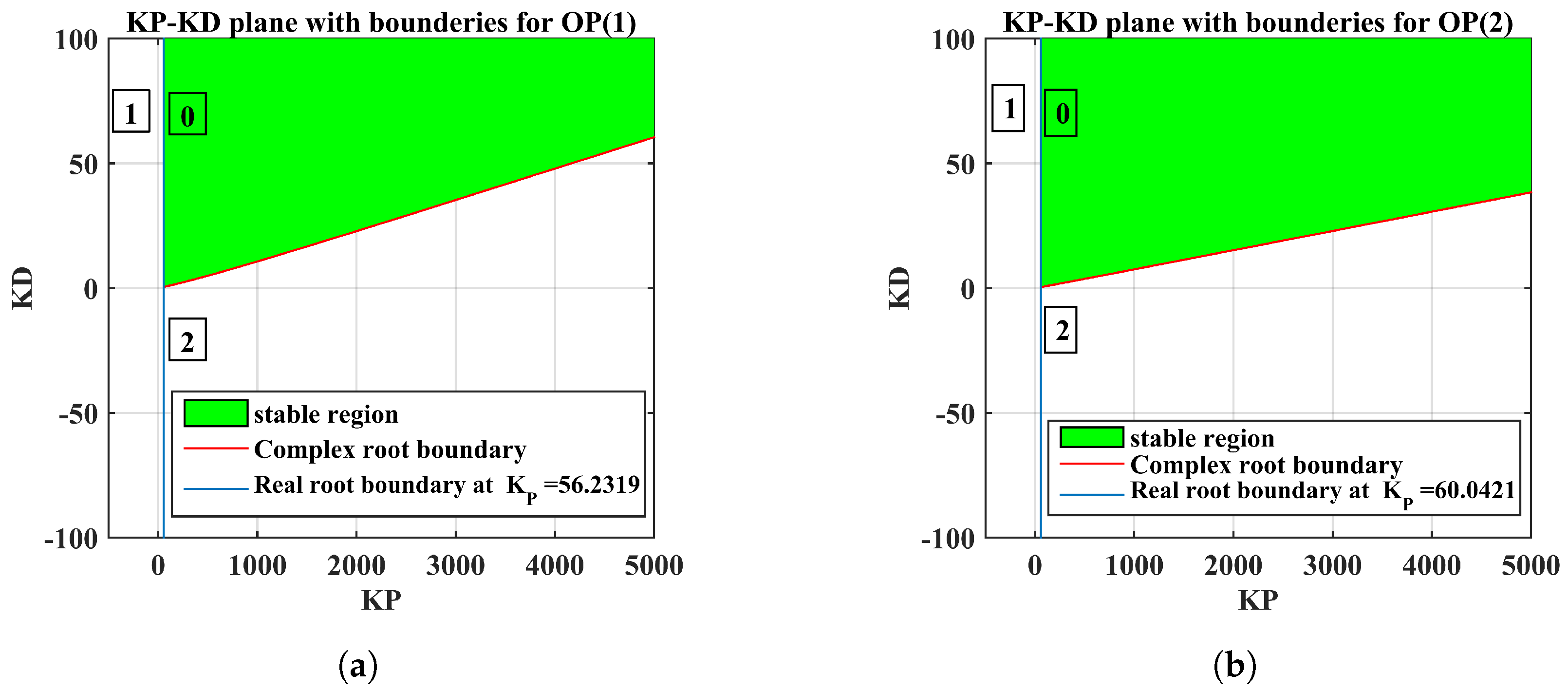
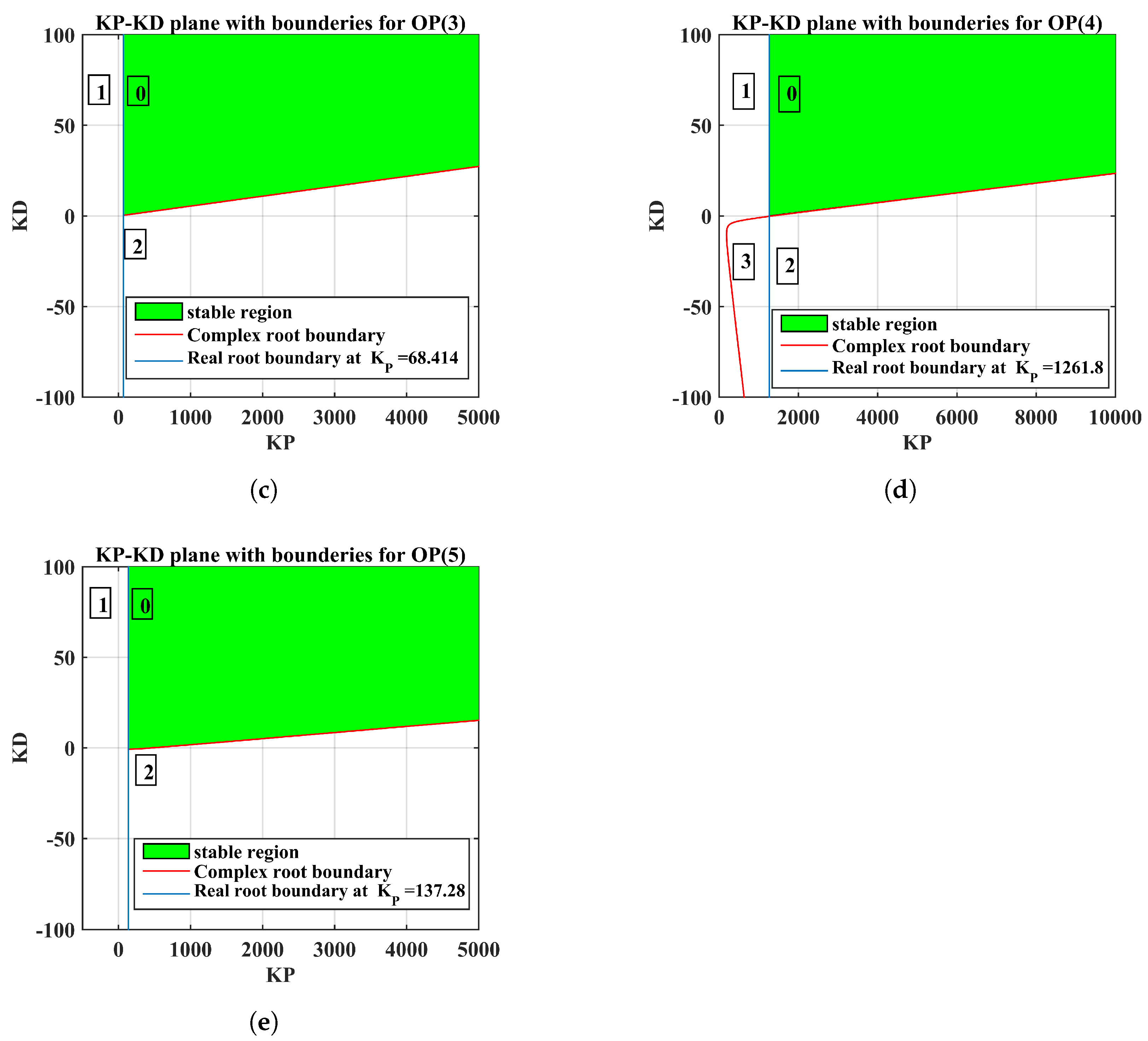
3. Stability Analysis

The proportional-derivative gain-scheduling Control system (PD-GS-C) solution based on the control system structure is shown in Figure 3, which can be considered the stabilizing control solution starting with the linearized state-space model in Equation (4).

Where the reference input is defined by r, the PD gain parameters are $K_p$ and $K_D$, and the ML2SEM model is described by the plant, which also contains the actuators and sensors. The minimum and maximum values of the PD gain controllers are typically set to limit the control action within certain bounds. By setting these limits, the control system can prevent excessive control efforts that could potentially destabilize the system or cause other undesirable effects. These values are used in equations of the proportional-derivative gain-scheduling control system (PD-GS-C), as shown in Section 4.2. The applied technique is based on a performance specification in terms of a parameter-space technique in order to determine the maximum and minimum of the PD gain controllers ($K_{pmax}$, $K_{Dmax}$, $K_{pmin}$, and $K_{Dmin}$), as shown in the next subsections.

Stabilizing Controller Gains

A parameter-space approach can be defined by the method of drawing lines that indicate the boundaries of the stabilizing gain set using the frequency response of the plant [54].

$G\left(s\right)$ is a single-input–single-output plant’s transfer function with a frequency response that can be illustrated by the following equation:

$$G\left(j\omega \right)=a\left(\omega \right)+jb\left(\omega \right),\omega \in \mathbb{R}$$

(7)

where $a,b$ are real-valued functions.

Equation (8) shows the transfer function of the proportional-derivative controller plant $G_{pd}\left(s\right)$.

$$G_{pd}\left(j\omega \right)=K_p+j\omega K_D,\omega \in \mathbb{R}$$

(8)

The characteristic equation of a closed-loop system with a PD controller is expressed as:

$$1+(K_p+j\omega K_D)(a\left(\omega \right)+jb\left(\omega \right))=0$$

(9)

Equation (9) can be rewritten in matrix form as:

$$\begin{array}{c}\left[\begin{array}{cc}a& -\omega b\\ b& \omega a\end{array}\right]\left[\begin{array}{c}{K}_P\\ K_D\end{array}\right]=\left[\begin{array}{c}-1\\ 0\end{array}\right]\hfill \end{array}$$

(10)

By solving Equations (9) or (10), $K_p$ and $K_D$ can be expressed by the following equation:

$$\begin{array}{c}{K}_p=\frac{-a}{a^2\left(\omega \right)+b^2\left(\omega \right)}\hfill \\ K_D=\frac{b}{\omega (a^2\left(\omega \right)+b^2\left(\omega \right))}\hfill \end{array}$$

(11)

When $\omega$ changes, the parameter plane can be separated into regions by drawing Equation (11) and the root real boundary line (at $\omega =0$). The number of unstable poles in each region is guaranteed to be kept fixed by the boundary-crossing theorem [55]. This characteristic allows us to calculate the stability set at each operating point [54,56,57]. The $K_P-K_D$ planes for operating points $p^{\left(1\right)}$, $p^{\left(2\right)}$, $p^{\left(3\right)}$, $p^{\left(4\right)}$, and $p^{\left(5\right)}$ are illustrated in Figure 4a–e, respectively.

Table 2. The stability of each zone for operating points $p^{\left(1\right)}$, $p^{\left(2\right)}$, $p^{\left(3\right)}$, $p^{\left(4\right)}$, and $p^{\left(5\right)}$.

${\mathit{p}}^{\left(\mathit{j}\right)}$	Test Point $\left[{\mathit{K}}_{\mathit{P}}{\mathit{K}}_{\mathit{D}}\right]$	System Poles	Number of Unstable Poles in a Specific Area	Stability of the Area
	[−100  5]	$1\times {10}^2$ * −2.4885 + 0.0000i −0.6406 + 2.0984i −0.6406 − 2.0984i 0.3144 + 0.0000i	1	unstable area
$P^{\left(1\right)}$	$\left[1005\right]$	$1\times {10}^2$ * −2.4722 + 0.0000i −0.4420 + 2.0257i −0.4420 − 2.0257i −0.0991 + 0.0000i	0	stable area
	$\left[10005\right]$	$1\times {10}^2$ * 0.3379 + 2.2962i 0.3379 − 2.2962i −2.2768 + 0.0000i −1.8542 + 0.0000i	2	unstable area
	$[-1005]$	$1\times {10}^2$ * −0.8189 + 1.9817i −0.8189 − 1.9817i −2.0321 + 0.0000i 0.3107 + 0.0000i	1	unstable area
$P^{\left(2\right)}$	$\left[1005\right]$	$1\times {10}^2$ * −2.0265 + 0.0000i −0.6212 + 1.8939i −0.6212 − 1.8939i −0.0901 + 0.0000i	0	stable area
	$\left[10005\right]$	$1\times {10}^2$ * 0.2069 + 2.1753i 0.2069 − 2.1753i −1.8864 + 0.1139i −1.8864 − 0.1139i	2	unstable area
	$[-1005]$	$1\times {10}^2$ * −1.0710 + 1.8602i −1.0710 − 1.8602i −1.5108 + 0.0000i 0.3105 + 0.0000i	1	unstable area
$P^{\left(3\right)}$	$\left[1005\right]$	$1\times {10}^2$ * −0.8812 + 1.7439i −0.8812 − 1.7439i −1.5089 + 0.0000i −0.0710 + 0.0000i	0	stable area
	$\left[10005\right]$	$1\times {10}^2$ * 0.0458 + 2.0269i 0.0458 − 2.0269i −1.9027 + 0.0000i −1.5311 + 0.0000i	2	unstable area
	$[-1005]$	$1\times {10}^2$ * −1.9547 + 1.8215i −1.9547 − 1.8215i 0.3581 + 0.0000i −0.2211 + 0.0000i	1	unstable area
$P^{\left(4\right)}$	$\left[20005\right]$	$1\times {10}^2$ * −3.2066 + 0.0000i −0.2722 + 2.1504i −0.2722 − 2.1504i −0.0213 + 0.0000i	0	stable area
	$[2000-5]$	$1\times {10}^2$ * −4.7157 + 0.0000i 0.4825 + 1.7053i 0.4825 − 1.7053i −0.0217 + 0.0000i	2	unstable area
	$[1000-5]$	$1\times {10}^2$ * −4.4271 + 0.0000i 0.3200 + 1.2076i 0.3200 − 1.2076i 0.0146 + 0.0000i	3	unstable area
	$[-1005]$	$1\times {10}^2$ * −1.6553 + 1.7938i −1.6553 − 1.7938i −0.5373 + 0.0000i 0.3268 + 0.0000i	1	unstable area
$P^{\left(5\right)}$	$\left[2005\right]$	$1\times {10}^2$ * −1.4543 + 1.5878i −1.4543 − 1.5878i −0.4857 + 0.0000i −0.1269 + 0.0000i	0	stable area
	$[200-5]$	−377.1251 −60.7665 67.2404 18.5370	2	unstable area

demonstrates the stability of each zone for operating points $p^{\left(1\right)}$, $p^{\left(2\right)}$, $p^{\left(3\right)}$, $p^{\left(4\right)}$, and $p^{\left(5\right)}$ by picking one polynomial for each region and testing its stability. The numbers (0, 1, 2, and 3) that appear in figures represent the number of unstable poles in the zone. The green zones in all figures represent the stable regions with zero unstable poles. In this research, the robust PD controller for $p^{\left(j\right)}$ is involved by computing all stabilizing PD controller gains for the characteristic polynomial using the parameter-space approach, as shown in Figure 4.

4. Controller Design

The results of the parameter-space approach are ranges of PD gains $(K_P,K_D)$. In the next subsection, the optimal PD gains were chosen using the Big Bang–Big Crunch Optimization Algorithm [58] to achieve optimal performance for ML2SEM magnetic levitation.

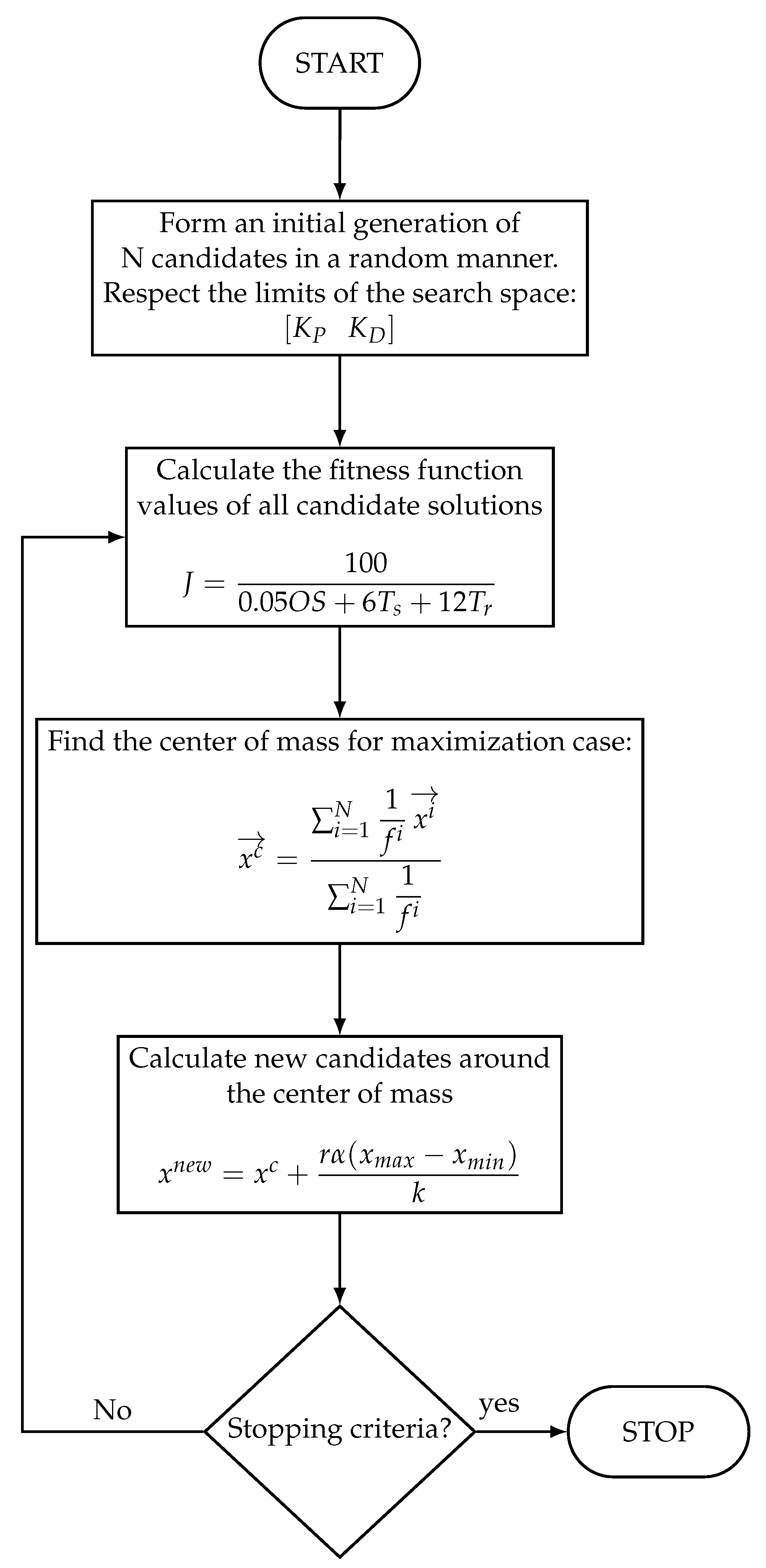
4.1. The Big Bang–Big Crunch Optimization Algorithm

The Big Bang–Big Crunch Optimization technique (BB-BC) is a population-oriented optimized algorithm that derives motivation from the cosmological events of the Big Bang and the Big Crunch. As a nature-inspired method for resolving challenging optimization issues, it was initially proposed by Erol and Eksin in 2006 [58]. The technique begins with a random population of candidate solutions that indicate potential solutions to the optimization challenge. Every potential solution is represented in the search space by a point. Depending on the scenario, the search space can be multidimensional. The BB-BC algorithm can be separated into two phases: the Big Bang phase and the Big Crunch phase.

• The Big Bang Phase: During the Big Bang phase, the candidate solutions are randomly spread throughout the search space, comparable to the exploded atoms during the Big Bang in cosmology. This phase is in control of exploration, allowing the solutions to cover a large portion of the search space.
• The Big Crunch Phase: Following the Big Bang phase, the algorithm initiates the Big Crunch phase, which depicts the contraction of matter in the universe, resulting in the construction of structures. During this phase, potential solutions are drawn to promising parts of the search space, identical to the development of galaxies and other cosmic structures. This phase focuses on exploitation, refining solutions, and convergence toward optimal solutions.
  The output of the Big Crunch phase can be defined as the center of mass. The center of mass is denoted by $\overrightarrow{x^c}$, which can be expressed as follows:

  $$\overrightarrow{x^c}={\displaystyle \frac{{\sum }_{i=1}^N{\displaystyle \frac{1}{f^i}}\overrightarrow{x^i}}{{\sum }_{i=1}^N{\displaystyle \frac{1}{f^i}}}}$$

  (12)

  where $\overrightarrow{x^i}$ and $\overrightarrow{x^c}$ are vectors in an n-dimensional search space, $f^i$ is the value of this point’s objective function, and N is the population size in the Big Bang phase.
  The following stage generates new points that are used in the Big Bang phase following the Big Crunch phase, generating the center of mass ($\overrightarrow{x^c}$). The newly generated points are redistributed in all directions around the center of mass ($\overrightarrow{x^c}$):

  $$x^{new}=\overrightarrow{x^c}+{\displaystyle \frac{r\alpha (x_{max}-x_{min})}{k}}$$

  (13)

  where r is a random number, $\alpha$ is a parameter that limits the size of the search space, and k is the number of iterations. [58,59,60,61,62].

Iterations during the Big Crunch phase drive candidate solutions closer to the best solutions in their area. Attractive forces guide the movements, which are determined by the fitness values of the solutions. Based on the performance function, the fitness function evaluates the level of accuracy of each solution.

The optimization approach is presented via a specific performance index function that is inversely proportional to a dynamical system’s time-domain step response criteria (small overshoot percentage $\left(OS\right)$ with significant minimization of both settling $\left(T_s\right)$ and rising $\left(T_r\right)$ times), which is demonstrated by Equation (14). A flow chart of the BB-BC optimization algorithm is shown in Figure 5.

$$J={\displaystyle \frac{100}{0.05OS+6T_s+12T_r}}$$

(14)

The search domains for $\left[K_P{K}_D\right]$ are shown in Figure 4 for each operating point.

Table 3. For the given system with alternative values of operating points, the performance varies in terms of overshot, rising time, settling time, peak time, and steady-state error.

${\mathit{P}}^{\left(\mathit{j}\right)}$	Lower Bounds $\left[{\mathit{K}}_{\mathit{P}}{\mathit{K}}_{\mathit{D}}\right]$	Upper Bounds $\left[{\mathit{K}}_{\mathit{P}}{\mathit{K}}_{\mathit{D}}\right]$	Optimal Values of $\left[{\mathit{K}}_{\mathit{P}}{\mathit{K}}_{\mathit{D}}\right]$	Value of the Cost Function	${\mathit{T}}_{\mathit{r}}$ (sec)	${\mathit{T}}_{\mathit{P}}$ (sec)	${\mathit{T}}_{\mathit{s}}$ (sec)	$\mathbf{OS}$	$\mathbf{SSE}$
$P^{\left(1\right)}$	$\left[50050\right]$	$\left[2000100\right]$	$\left[56850\right]$	$23.26$	$0.0018$	$0.0048$	$0.1512$	$58.7$	$0.1085$
$P^{\left(2\right)}$	$\left[50050\right]$	$\left[2000100\right]$	$\left[71650\right]$	$26.56$	$0.0018$	$0.0048$	$0.0980$	$63.1$	$0.0805$
$P^{\left(3\right)}$	$\left[50050\right]$	$\left[2000100\right]$	$\left[86750\right]$	$30.77$	$0.0019$	$0.0049$	$0.0717$	$56.0$	$0.0846$
$P^{\left(4\right)}$	$\left[400050\right]$	$\left[8000100\right]$	$\left[693466\right]$	$23.22$	$0.0020$	$0.0048$	$0.4870$	$27.2$	$0.2142$
$P^{\left(5\right)}$	$\left[50050\right]$	$\left[4000100\right]$	$\left[101250\right]$	$47.46$	$0.0230$	$0.0053$	$0.1650$	$28.8$	$0.1455$

demonstrates that the performance varies in terms of overshoot ($OS$), rise time ($T_r$), settling time ($T_s$), peak time ($T_P$), and steady-state error ($SSE$) for the five operating points. In addition, the optimal values of the PD gain controller, as well as the maximum and minimum gains for each of the five operating points, are shown in Table 3. Furthermore, Figure 6 shows the step response of the optimal PD gains controllers obtained by employing the BB-BC algorithm for each of the five operating points.

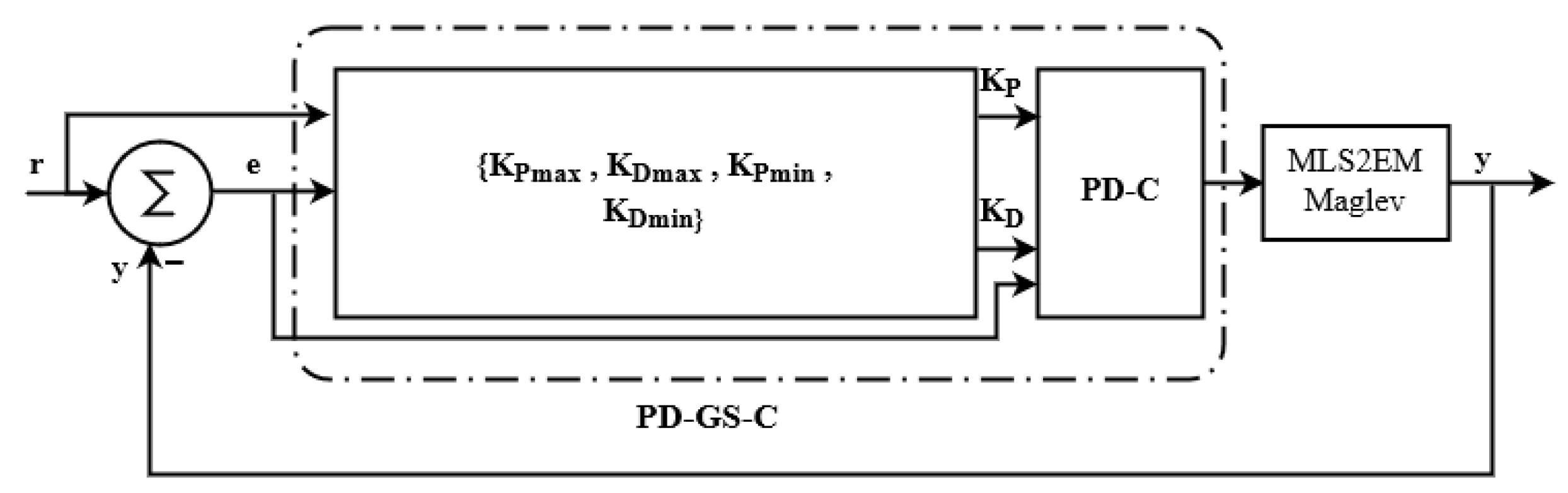
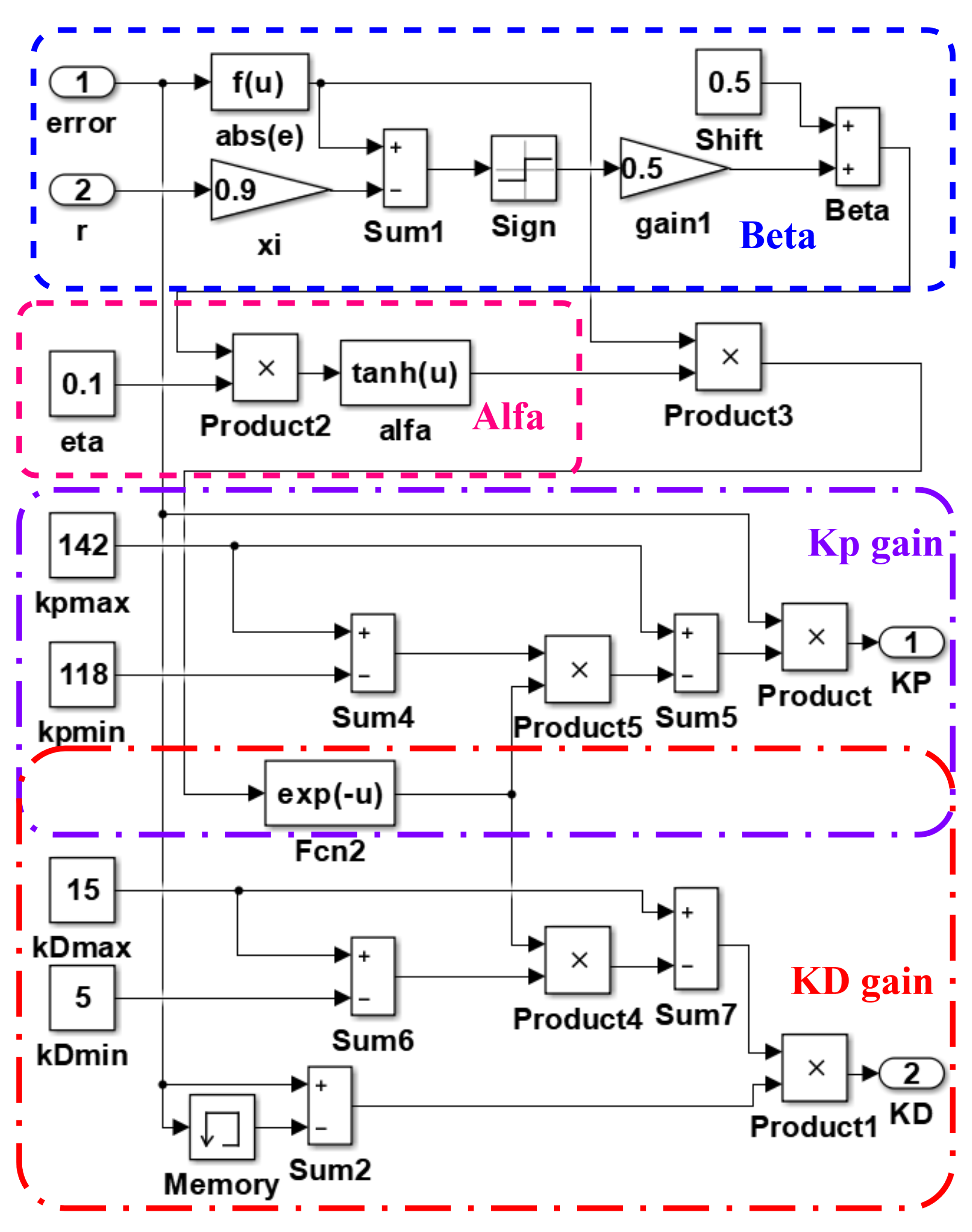
4.2. The Proportional-Derivative Gain-Scheduling Controller (PD-GS-C)

According to [63], swapping from one PD control scheme to another is a sensible way to guarantee improved performance, although process nonlinearities depend on the operating point as well. This method is defined as the PD gain schedule. Figure 3 depicts the gain-scheduling PD voltage controller used in magnetic levitation. It is mathematically represented by Equation (15).

$$\Delta u_1\left(t\right)=K_{P}e\left(t\right)+K_D\frac{de\left(t\right)}{dt}$$

(15)

where the proportional gain ($K_P\left(t\right)$) and the derivative gain ($K_D\left(t\right)$) are functions of $e\left(t\right)$ such that $e\left(t\right)=r\left(t\right)-y\left(t\right)$. The following mathematical formula can be used to define the proportional gain ($K_P\left(t\right)$) and the derivative gain ($K_D\left(t\right)$) as a function of e(t) [46]:

$$\begin{array}{c}{K}_P\left(t\right)=K_{P_{max}}-(K_{P_{max}}-K_{P_{min}})exp(-(\alpha \left(t\right)|e\left(t\right)\left|\right)),\hfill \\ K_D\left(t\right)=K_{D_{max}}-(K_{D_{max}}-K_{D_{min}})exp(-(\alpha \left(t\right)|e\left(t\right)\left|\right)).\hfill \end{array}$$

(16)

where $0\le \alpha \left(t\right)\le 1$ and $K_{P_{max}}$, $K_{P_{min}}$, $K_{D_{max}}$, and $K_{D_{min}}$ are the maximum and minimum values of the proportional gain ($K_P$) and the derivative gain ($K_D$), respectively.

Equation (16) demonstrates that the exponential term approaches zero $\left(exp\right(-\left(\alpha \right(t\left)\right|e\left(t\right)\left|\right))$$\to 0)$ when $e\left(t\right)$ is large. Consequentially, $K_P\left(t\right)=K_{P_{max}}$. Similarly, when the error ($e\left(t\right)$) is minimal, the exponential term approaches one $\left(exp\right(-\left(\alpha \right(t\left)\right|e\left(t\right)\left|\right))\to 1)$, and as a result, $K_P\left(t\right)=K_{P_{min}}$.

In this modification, $K_P$ and $K_D$ are evaluated by the control scheme so that when the error ($e\left(t\right)$) is large, we predict maximum proportional and derivative gains ($K_{P_{max}}$ and $K_{D_{max}}$) to enhance the control signal’s voltage up to the dynamic response, and when the error ($e\left(t\right)$) is small, we anticipate minimal proportional derivative gains ($K_{P_{min}}$ and $K_{D_{min}}$) to overcome the unfavorable issue of overshoot. These fluctuation in the gains are generated by the variable “$\alpha \left(t\right)$” to determine how quickly $K_P\left(t\right)$ and $K_P\left(t\right)$ change between the maximum and minimum values [63].

In order to transfer from one PD controller to another using a smooth and steady method, the parameter $0\le \alpha \left(t\right)\le 1$ is included. To determine this parameter’s value, the following equation is applied:

$$\alpha \left(t\right)=tanh\left(\eta \beta \right(t\left)\right)=\frac{\left(exp\right(2\eta \beta \left(t\right))-1)}{\left(exp\right(2\eta \beta \left(t\right))+1)}$$

(17)

where the factor $\eta$ was selected to guarantee specific dynamics of the fluctuation of $\alpha \left(t\right)$ and specifies the rate at which $\alpha \left(t\right)$ varies from 0 to 1. The variable $\beta \left(t\right)$ is defined in terms of $\left|e\right(t\left)\right|$ and $r\left(t\right)$ [46]:

$$\beta \left(t\right)=\left\{\begin{array}{ccc}\hfill 1,& \mathrm{for}\hfill & \left|e\right(t\left)\right|>\xi \hfill \\ \hfill 0,& \mathrm{for}\hfill & \left|e\right(t\left)\right|\le \xi \hfill \end{array}\right.,\xi =0.9.r\left(t\right)$$

(18)

where the parameter $\xi$ is set according to [46].

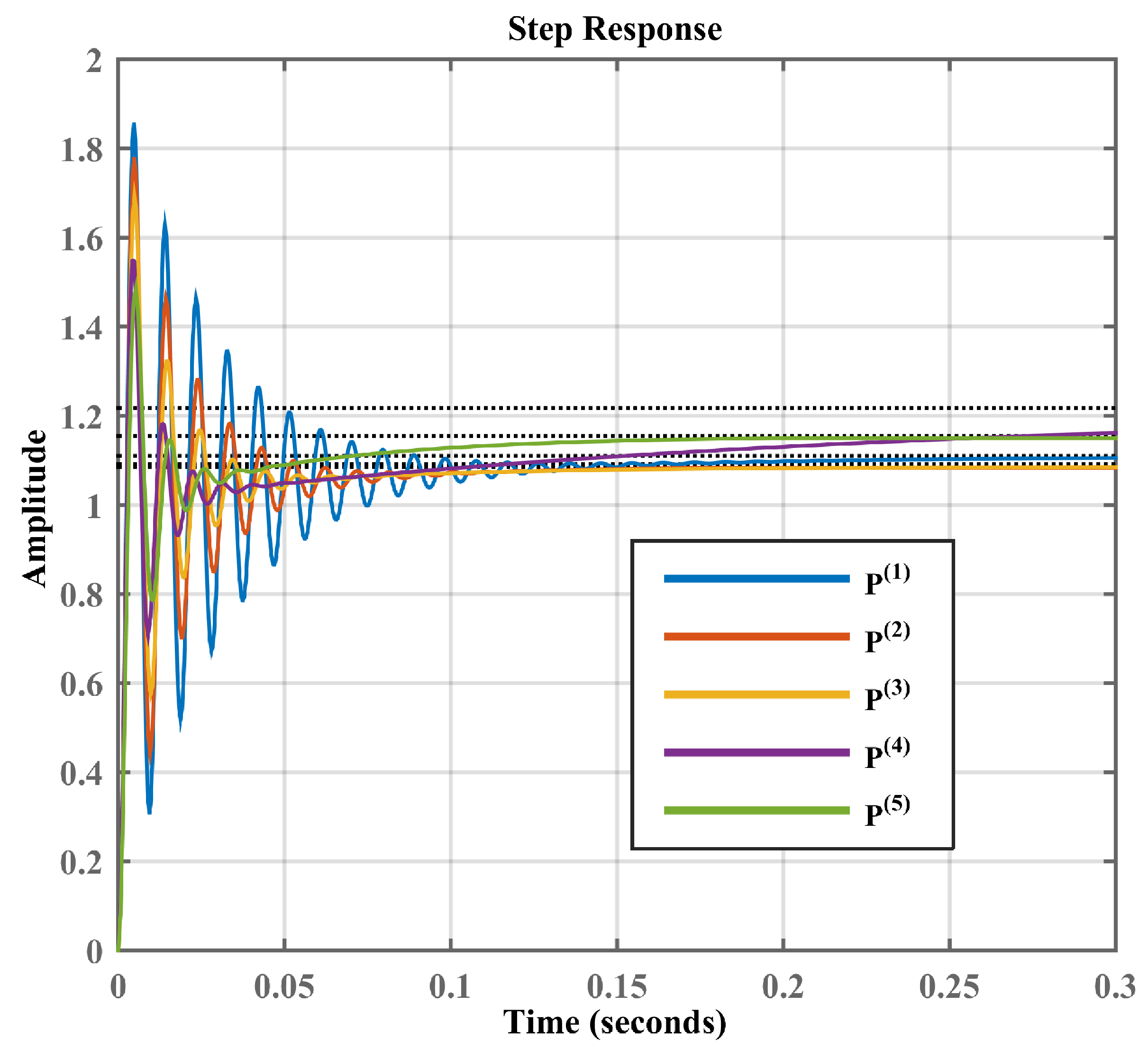
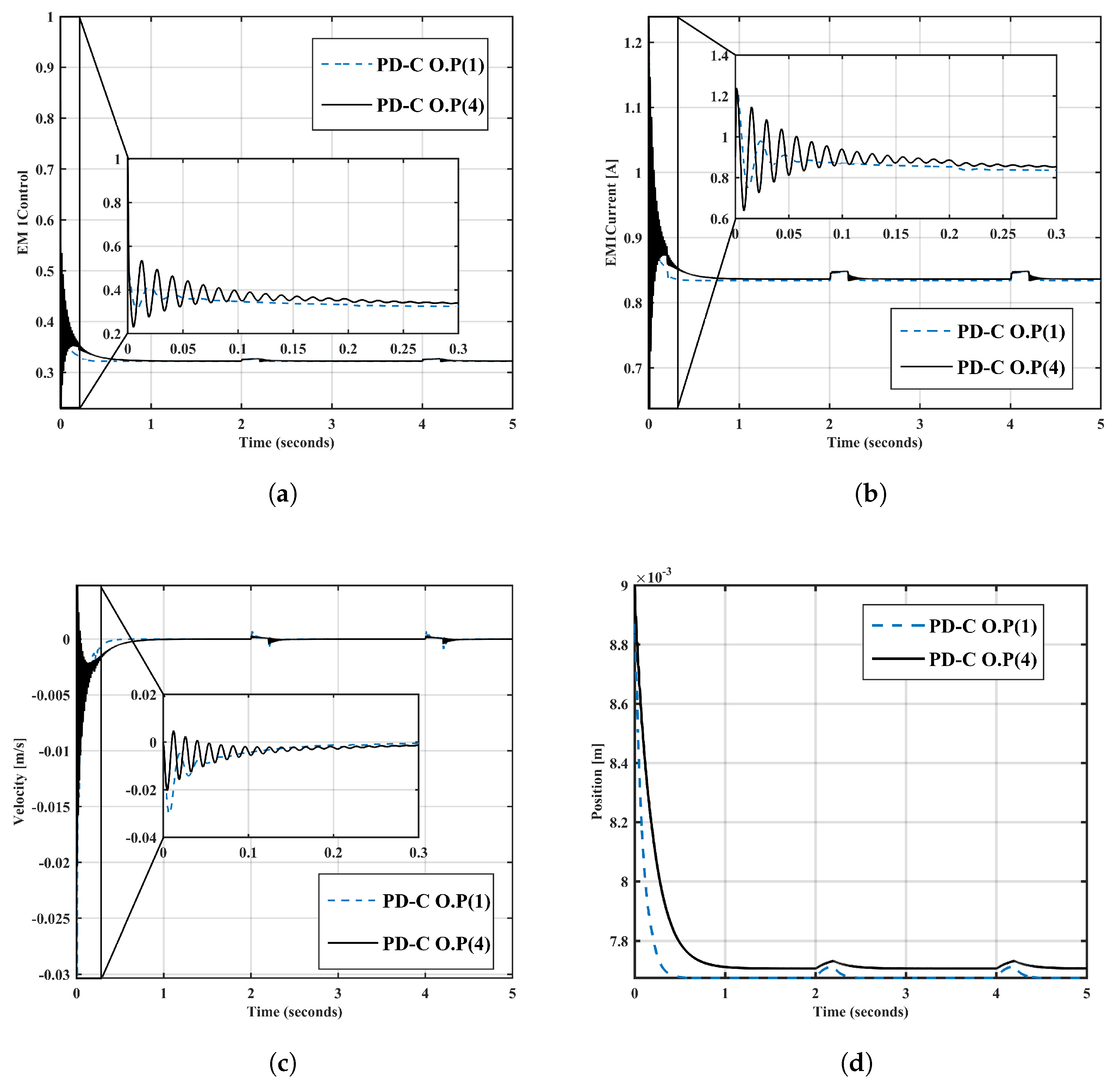
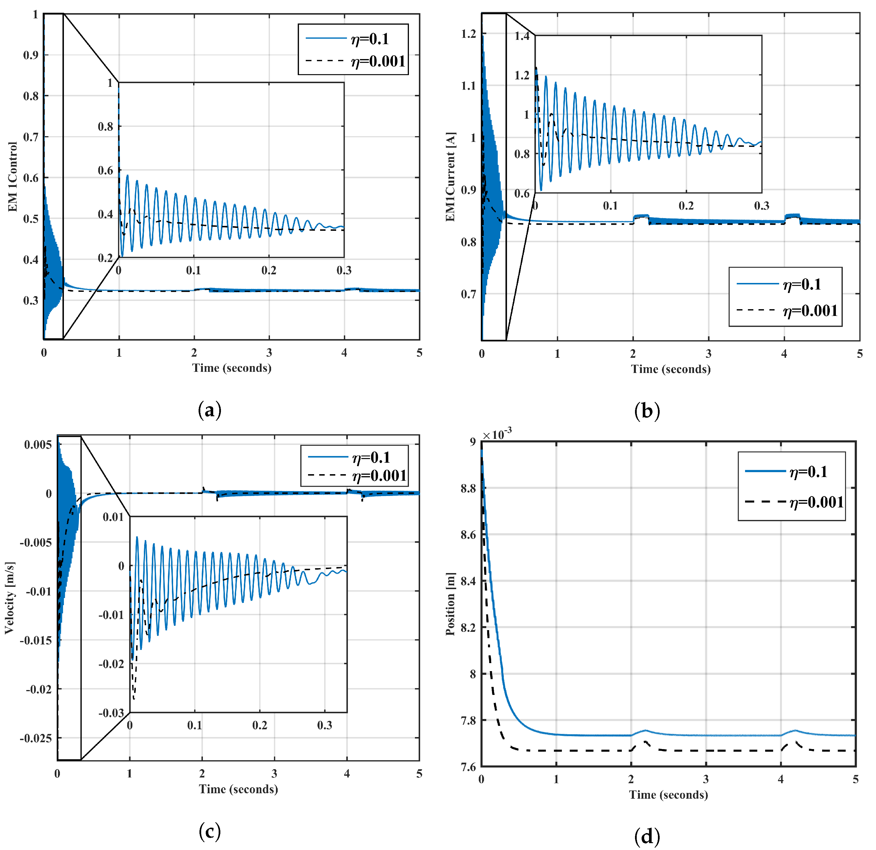
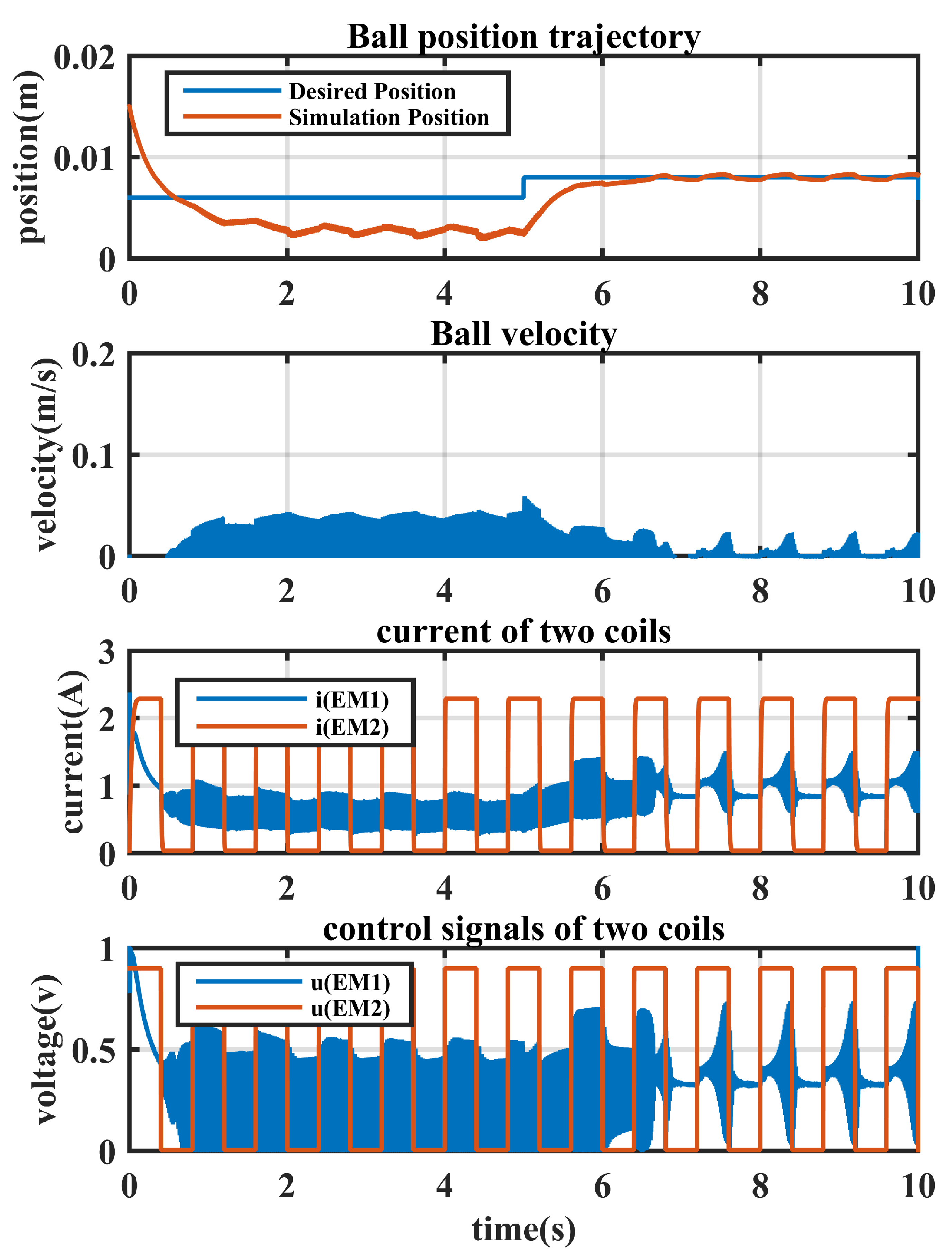
5. Simulation Results

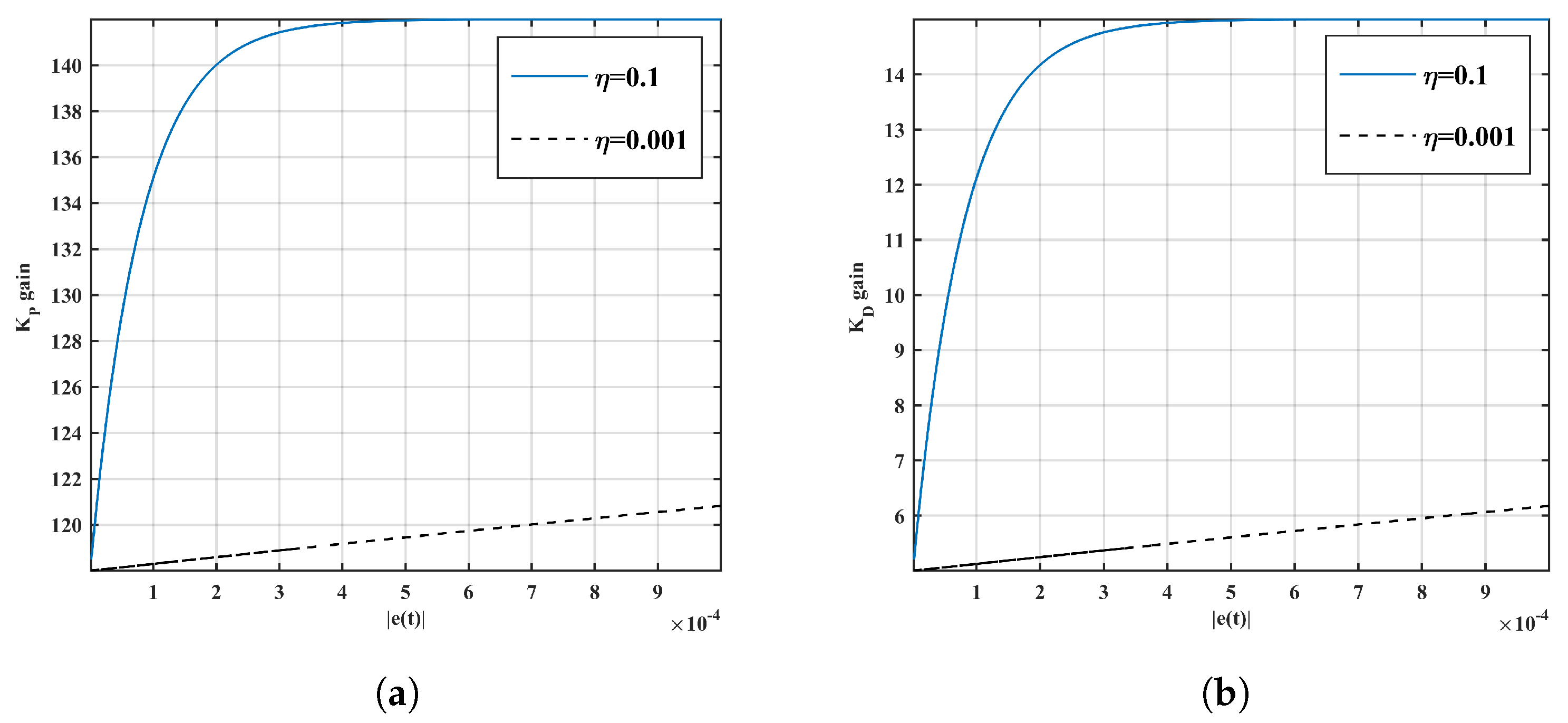
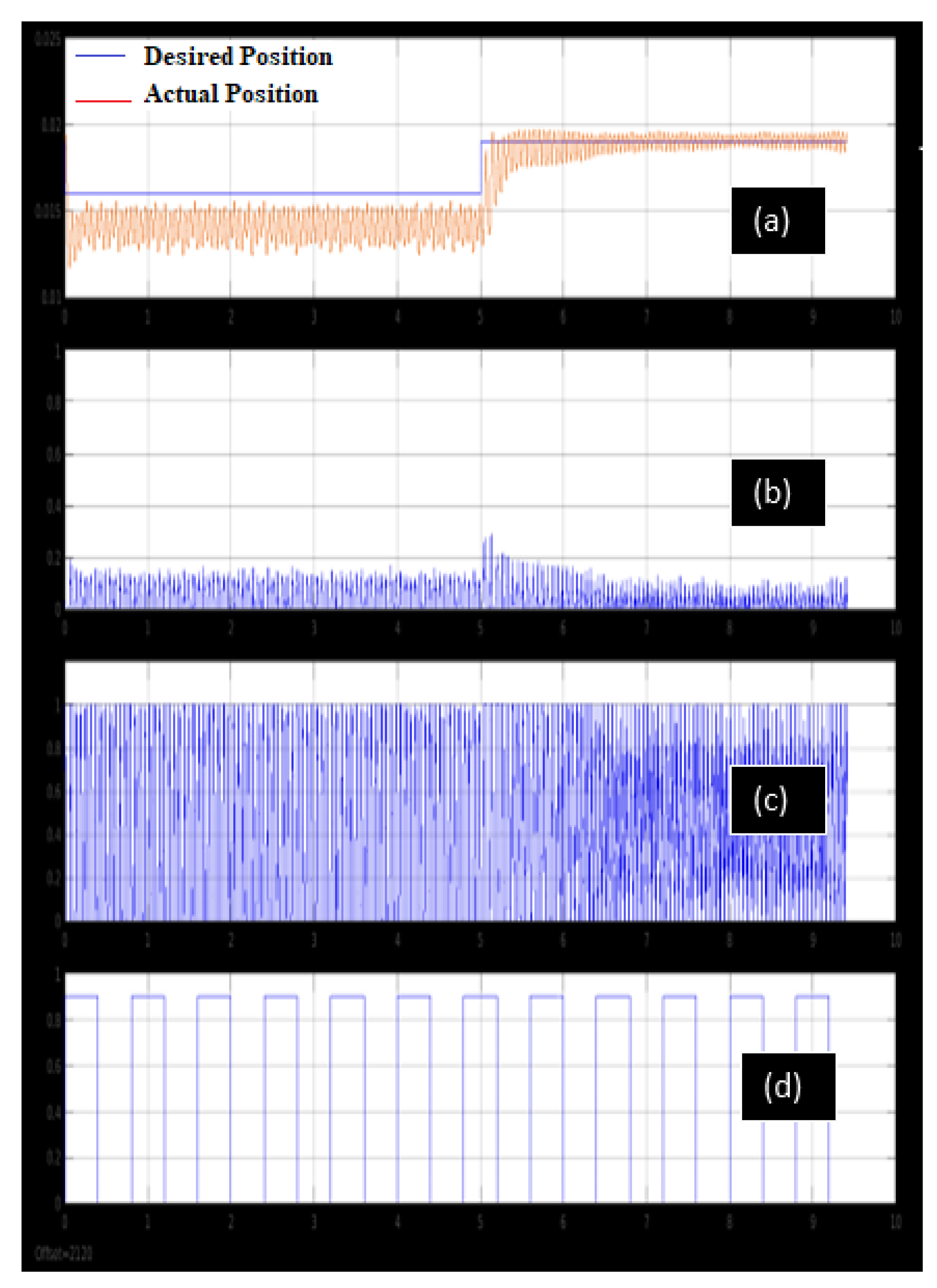
Simulink in MATLAB(R2015a) was used to simulate the two control mechanisms: the optimal PD-C and PD-GS-C. Figure 7 demonstrates the control mechanism of PD-GS-C by Simulink(R2015a). The reference input in each scenario was a signal that was set to $0.008$ m from the upper coil, and the responses of the controls were examined during a time period of 5 s. Graphs of the top electromagnet’s responses to the ball location, ball velocity, coil current, and control signal are presented.

A PD controller with five operating points was simulated in MATLAB(R2015a). The simulation results of the control system with a PD controller developed specifically for the two o.p.s ($\left(1\right)$ and $\left(4\right)$) are presented in Figure 8a, which shows the control signal over time. The time-varying coil current through EM1 is displayed in Figure 8b, the ball velocity is shown in Figure 8c, and Figure 8d demonstrates the controlled output position of ball over time.

The results show that the system’s nonlinear effects generate oscillations at the start of transient responses.

The specifications of the PD-GS-C component in Figure 3 have the variables $K_{P_{max}}$, $K_{P_{min}}$, $K_{D_{max}}$, and $K_{D_{min}}$. By using the optimal values from Table 3, $\eta =\in [0.001,0.1]$. These values were obtained using the big bang–big crunch optimization technique (BB-BC) in the context of a tradeoff for overshoot for the five operating points.

The conditions listed below can be taken into consideration when designing the PD-GS-C structure:

• $K_{P_{min}}$ and $K_{D_{min}}$ are enabled during the steady state to achieve a minimal value of steady-state error ($\left|e\right(t\left)\right|$) to resolve the unacceptable challenge of overshoot as shown in Figure 9.
• $K_{P_{max}}$ and $K_{D_{max}}$ are generated when the process steady-state error $\left|e\right(t\left)\right|$ is large in order to provide a significant control signal and to mitigate unfavorable fluctuation and error, as illustrated in Figure 9.

Figure 10 illustrates responses to various variables estimated in the proposed scheme. The simulation results of the control system using the PD-GS controller are presented in Figure 10a, which shows the control signal over time. The time-varying coil current through EM1 is displayed in Figure 10b, and the ball velocity is shown in Figure 10c. Moreover, Figure 10d shows the controlled output over time.

Due to the PD-GS controller’s optimized dynamic response, which is characterized by fewer oscillations and less settling time, its results are superior to those shown in Figure 8. MATLAB simulation and nonlinear laboratory equipment were used to test and validate the PD-C and PD-GS-C control structures in real-time experiments. Figure 11 shows the MATLAB simulation results of a robust proportional-derivative gain-scheduling controller (PD-GS -C).

Figure 12 displays the real-time experimental results of a robust Proportional-derivative gain-scheduling controller (PD-GS-C). Significant agreement was observed between theoretical and practical observations.

6. Conclusions

Two control schemes (PD-C and (PD-GS-C) were been designed to control the orientation of a ball in an MLS2EM system. The PD-C (proportional-derivative controller) is a straightforward control scheme that uses the proportional and derivative terms to control the system’s orientation. The PD controller was designed based on a linearized model of MLS2EM around five operating points, allowing for the application of conventional control techniques. The PD-GS-C (proportional-derivative with gain scheduling controller) was designed to switch between multiple PD controllers based on specific conditions. To achieve this, a parameter-space approach was employed to design five robust PD controllers with varying gains ($K_P$ and $K_D$). The ranges of PD gains obtained using the parameter-space approach were used in the PD-GS-C structure, allowing the controller to adapt its gains according to different operating conditions. To find the optimal PD gains for the PD-GS-C controller, we utilized the big bang–big crunch optimization technique (BB-BC). This optimization method was applied to improve the system’s performance in terms of time-domain step response criteria, which include minimizing overshoot percentage, settling time, and rising time. The performance index function was defined to quantify the desired performance criteria, and the optimization process aims to maximize this index function, thereby optimizing the system’s performance. To evaluate the effectiveness of the proposed control schemes, both PD-C and PD-GS-C configurations were tested using Simulink/MATLAB simulations, as well as real-time experiments. By comparing the PD-GS controller with the conventional PD controller, this research demonstrates the efficacy of the PD-GS-C scheme in achieving optimal control performance for an MLS2EM magnetic levitation system. As the gain-scheduling approach provided good results, we intend to extend this idea to other controller configurations, such as PI and PID controls. Therefore, in future research, a comparison of gain-scheduled PI/PD/PID controllers will be conducted under the same scenario of operating points and controller scheduling. An interesting approach to be considered in future research is that of finite-time control. Finite-time control strategies aim to achieve desired control objectives within a specified time frame, which can be particularly beneficial for systems wherein rapid and precise control is crucial. Magnetic levitation systems often require precise control to maintain stable levitation and positioning of objects, making them a suitable candidate for such research.

References

1. Sinha, P.K. Electromagnetic Suspension Dynamics & Control; Savoy Place: London, UK, 1987. [Google Scholar]
2. Czerwiński, K.; Ławryńczuk, M. Identification of discrete-time model of active magnetic levitation system. In Proceedings of the Trends in Advanced Intelligent Control, Optimization and Automation: Proceedings of KKA 2017—The 19th Polish Control Conference, Kraków, Poland, 18–21 June 2017; pp. 599–608.
3. Sun, Z. Magnetic Levitation Based on Switched Reluctance Actuator. Ph.D. Thesis, Hong Kong Polytechnic University, Hong Kong, China, 2011. [Google Scholar]
4. Almobaied, M.; Al-Nahhal, H.S.; Issa, K.B. Computation of stabilizing PID controllers for magnetic levitation system with parametric uncertainties. In Proceedings of the 2021 International Conference on Electric Power Engineering–Palestine (ICEPE-P), Gaza, Palestine, 23–24 March 2021; pp. 1–7. [Google Scholar]
5. Bojan-Dragos, C.A.; Stinean, A.I.; Precup, R.E.; Preitl, S.; Petriu, E.M. Model predictive control solution for magnetic levitation systems. In Proceedings of the 2015 20th International Conference on Methods and Models in Automation and Robotics (MMAR), Miedzyzdroje, Poland, 24–27 August 2015; pp. 139–144. [Google Scholar]
6. Eroğlu, Y.; Ablay, G. Cascade sliding mode-based robust tracking control of a magnetic levitation system. Proc. Inst. Mech. Eng. Part I J. Syst. Control Eng. 2016, 230, 851–860. [Google Scholar] [CrossRef]
7. El Hajjaji, A.; Ouladsine, M. Modeling and nonlinear control of magnetic levitation systems. IEEE Trans. Ind. Electron. 2001, 48, 831–838. [Google Scholar] [CrossRef]
8. Barie, W.; Chiasson, J. Linear and nonlinear state-space controllers for magnetic levitation. Int. J. Syst. Sci. 1996, 27, 1153–1163. [Google Scholar] [CrossRef]
9. Beltran-Carbajal, F.; Valderrabano-Gonzalez, A.; Rosas-Caro, J.; Favela-Contreras, A. Output feedback control of a mechanical system using magnetic levitation. ISA Trans. 2015, 57, 352–359. [Google Scholar] [CrossRef] [PubMed]
10. Morales, R.; Sira-Ramírez, H. Trajectory tracking for the magnetic ball levitation system via exact feedforward linearisation and GPI control. Int. J. Control 2010, 83, 1155–1166. [Google Scholar] [CrossRef]
11. Nielsen, C.; Fulford, C.; Maggiore, M. Path following using transverse feedback linearization: Application to a maglev positioning system. Automatica 2010, 46, 585–590. [Google Scholar] [CrossRef]
12. Zhang, J.; Tao, T.; Mei, X.; Jiang, G.; Zhang, D. Non-linear robust control of a voltage-controlled magnetic levitation system with a feedback linearization approach. Proc. Inst. Mech. Eng. Part I J. Syst. Control Eng. 2011, 225, 85–98. [Google Scholar] [CrossRef]
13. El Rifai, O.M.; Youcef-Toumi, K. Achievable performance and design trade-offs in magnetic levitation control. In Proceedings of the AMC’98-Coimbra—1998 5th International Workshop on Advanced Motion Control, Coimbra, Portugal, 29 June–1 July 1998; pp. 586–591. [Google Scholar]
14. Hasirci, U.; Balikci, A.; Zabar, Z.; Birenbaum, L. A novel magnetic-levitation system: Design, implementation, and nonlinear control. IEEE Trans. Plasma Sci. 2010, 39, 492–497. [Google Scholar] [CrossRef]
15. Baranowski, J.; Piątek, P. Observer-based feedback for the magnetic levitation system. Trans. Inst. Meas. Control 2012, 34, 422–435. [Google Scholar] [CrossRef]
16. Al-Araji, A.S. Cognitive non-linear controller design for magnetic levitation system. Trans. Inst. Meas. Control 2016, 38, 215–222. [Google Scholar] [CrossRef]
17. Benitez-Pérez, H.; Ortega-Arjona, J.; Cardenas-Flores, F.; Quiñones-Reyes, P. Reconfiguration control strategy using Takagi–Sugeno model predictive control for network control systems—A magnetic levitation case study. Proc. Inst. Mech. Eng.-Part I J. Syst. Control Eng. 2010, 224, 1022. [Google Scholar] [CrossRef]
18. Chen, S.Y.; Lin, F.J.; Shyu, K.K. Direct decentralized neural control for nonlinear MIMO magnetic levitation system. Neurocomputing 2009, 72, 3220–3230. [Google Scholar] [CrossRef]
19. Cho, D.; Kato, Y.; Spilman, D. Sliding mode and classical controllers in magnetic levitation systems. IEEE Control Syst. Mag. 1993, 13, 42–48. [Google Scholar]
20. Al-Muthairi, N.; Zribi, M. Sliding mode control of a magnetic levitation system. Math. Probl. Eng. 2004, 2004, 93–107. [Google Scholar] [CrossRef]
21. Lin, F.J.; Chen, S.Y.; Shyu, K.K. Robust dynamic sliding-mode control using adaptive RENN for magnetic levitation system. IEEE Trans. Neural Networks 2009, 20, 938–951. [Google Scholar] [PubMed]
22. Lin, F.J.; Teng, L.T.; Shieh, P.H. Intelligent adaptive backstepping control system for magnetic levitation apparatus. IEEE Trans. Magn. 2007, 43, 2009–2018. [Google Scholar] [CrossRef]
23. Bächle, T.; Hentzelt, S.; Graichen, K. Nonlinear model predictive control of a magnetic levitation system. Control Eng. Pract. 2013, 21, 1250–1258. [Google Scholar] [CrossRef]
24. Iplikci, S.; Bahtiyar, B. A field-programmable gate array implementation of a real-time nonlinear Runge–Kutta model predictive control. Trans. Inst. Meas. Control 2016, 38, 555–564. [Google Scholar] [CrossRef]
25. Javadi, A.; Pezeshki, S. A new model-free adaptive controller versus non-linear H∞ controller for levitation of an electromagnetic system. Trans. Inst. Meas. Control 2013, 35, 321–329. [Google Scholar] [CrossRef]
26. Kumar, E.V.; Jerome, J. LQR based optimal tuning of PID controller for trajectory tracking of magnetic levitation system. Procedia Eng. 2013, 64, 254–264. [Google Scholar] [CrossRef]
27. Wang, B.; Liu, G.P.; Rees, D. Networked predictive control of magnetic levitation system. In Proceedings of the 2009 IEEE International Conference on Systems, Man and Cybernetics, San Antonio, TX, USA, 11–14 2009; pp. 4100–4105. [Google Scholar]
28. An, S.; Ma, Y.; Cao, Z. Applying simple adaptive control to magnetic levitation system. In Proceedings of the 2009 Second International Conference on Intelligent Computation Technology and Automation, Zhangjiajie, China, 10–11 October 2009; Volume 1, pp. 746–749. [Google Scholar]
29. Ziętkiewicz, J. Constrained predictive control of a levitation system. In Proceedings of the 2011 16th International Conference on Methods & Models in Automation & Robotics, Miedzyzdroje, Poland, 22–25 August 2011; pp. 278–283. [Google Scholar]
30. Chauhan, S.; Nigam, M. Model predictive controller design and perturbation study for magnetic levitation system. In Proceedings of the 2014 Recent Advances in Engineering and Computational Sciences (RAECS), Chandigarh, India, 6–8 March 2014; pp. 1–6. [Google Scholar]
31. King, R.; Stathaki, A. Fuzzy gain-scheduling control of nonlinear processes. In Proceedings of the WSES/IEEE/IMACS World Multiconference on Circuits, Systems, Communications and Computers CSCC’99, Athens, Greece, 4–8 July 1999. [Google Scholar]
32. Huang, Y.W.; Tung, P.C. Design of a fuzzy gain scheduling controller having input saturation: A comparative study. J. Mar. Sci. Technol. 2009, 17, 249–256. [Google Scholar] [CrossRef]
33. Elsodany, N.M.; Rezeka, S.F.; Maharem, N.A. Adaptive PID control of a stepper motor driving a flexible rotor. Alex. Eng. J. 2011, 50, 127–136. [Google Scholar] [CrossRef]
34. Bianchi, F.D.; Peña, R.S.S. Interpolation for gain-scheduled control with guarantees. Automatica 2011, 47, 239–243. [Google Scholar] [CrossRef]
35. Zhao, Z.Y.; Tomizuka, M.; Isaka, S. Fuzzy gain scheduling of PID controllers. IEEE Trans. Syst. Man Cybern. 1993, 23, 1392–1398. [Google Scholar] [CrossRef]
36. Ye, Z.; Zhang, D.; Deng, C.; Yan, H.; Feng, G. Finite-time resilient sliding mode control of nonlinear UMV systems subject to DoS attacks. Automatica 2023, 156, 111170. [Google Scholar] [CrossRef]
37. Lashin, M.; Elgammal, A.T.; Ramadan, A.; Abouelsoud, A.; Assal, S.F.; Abo-Ismail, A. Fuzzy-based gain scheduling of Exact FeedForward Linearization control and sliding mode control for magnetic ball levitation system: A comparative study. In Proceedings of the 2014 IEEE International Conference on Automation, Quality and Testing, Robotics, Cluj-Napoca, Romania, 22–24 May 2014; pp. 1–6. [Google Scholar]
38. Michino, R.; Tanaka, H.; Mizumoto, I. Application of high gain adaptive output feedback control to a magnetic levitation system. In Proceedings of the 2009 ICCAS-SICE, Fukuoka City, Japan, 18–21 August 2009; pp. 970–975. [Google Scholar]
39. Puig, V.; Bolea, Y.; Blesa, J. Robust gain-scheduled Smith PID controllers for second order LPV systems with time varying delay. IFAC Proc. Vol. 2012, 45, 199–204. [Google Scholar] [CrossRef]
40. Bianchi, F.D.; Sánchez-Peña, R.S.; Guadayol, M. Gain scheduled control based on high fidelity local wind turbine models. Renew. Energy 2012, 37, 233–240. [Google Scholar] [CrossRef]
41. Yang, Y.; Yan, Y. Attitude regulation for unmanned quadrotors using adaptive fuzzy gain-scheduling sliding mode control. Aerosp. Sci. Technol. 2016, 54, 208–217. [Google Scholar] [CrossRef]
42. Bedoud, K.; Ali-rachedi, M.; Bahi, T.; Lakel, R. Adaptive Fuzzy Gain Scheduling of PI Controller for Control of the Wind Energy Conversion Systems. Energy Procedia 2015, 74, 211–225. [Google Scholar] [CrossRef]
43. Dounis, A.I.; Kofinas, P.; Alafodimos, C.; Tseles, D. Adaptive fuzzy gain scheduling PID controller for maximum power point tracking of photovoltaic system. Renew. Energy 2013, 60, 202–214. [Google Scholar] [CrossRef]
44. Xie, Y.; Shi, H.; Alleyne, A.G.; Yang, B. Feedback shape control for deployable mesh reflectors using gain scheduling method. Acta Astronaut. 2016, 121, 241–255. [Google Scholar] [CrossRef]
45. Bojan-Dragos, C.A.; Precup, R.E.; Preitl, S.; Hergane, S.; Hughiet, E.G.; Szedlak-Stinean, A.I. proportional–integral gain-scheduling control of a magnetic levitation system. In Proceedings of the 2016 20th International Conference on System Theory, Control and Computing (ICSTCC), Sinaia, Romania, 13–15 October 2016; pp. 1–6. [Google Scholar]
46. Bojan-Dragos, C.A.; Precup, R.E.; Tomescu, M.L.; Preitl, S.; Tanasoiu, O.M.; Hergane, S. proportional–integral-derivative gain-scheduling control of a magnetic levitation system. Int. J. Comput. Commun. Control 2017, 12, 599–611. [Google Scholar] [CrossRef]
47. Alfaro, V.M.; Vilanova, R. Model-Reference Robust Tuning of PID Controllers; Springer: Berlin/Heidelberg, Germany, 2016. [Google Scholar]
48. Rojas, J.D.; Arrieta, O.; Vilanova, R. Industrial PID Controller Tuning; Springer: Berlin/Heidelberg, Germany, 2021. [Google Scholar]
49. Aryan, P.; Raja, G.L.; Vilanova, R. Optimal iIMC-PD double-loop control strategy for integrating processes with dead-time. In Proceedings of the APCA International Conference on Automatic Control and Soft Computing, Caparica, Portugal, 6–8 July 2022; pp. 521–531. [Google Scholar]
50. Arrieta, O.; Vilanova, R. Servo/Regulation tradeoff tuning of PID controllers with a robustness consideration. In Proceedings of the 2007 46th IEEE Conference on Decision and Control, New Orleans, LA, USA, 12–14 December 2007; pp. 1838–1843. [Google Scholar]
51. Arrieta, O.; Vilaxova, R. Performance degradation analysis of controller tuning modes: Application to an optimal PID tuning. Int. J. Innov. Comput. Inf. Control 2010, 6, 4719–4729. [Google Scholar]
52. Magnetic Levitation System 2EM (MLS2EM) User’s Manual; Inteco Ltd.: Sankt-Petersburg, Russia, 2008.
53. Dragoş, C.A.; Precup, R.E.; Preitl, S.; Petriu, E.M.; Rădac, M.B. Control Solutions, Simulation and Experimental Results for a Magnetic Levitation Laboratory System. Available online: https://www.eurosim.info/fileadmin/user_upload_eurosim/EUROSIM_OA/Congress/2010/data/papers/155.pdf (accessed on 7 September 2023).
54. Saeki, M. Properties of stabilizing PID gain set in parameter space. IEEE Trans. Autom. Control 2007, 52, 1710–1715. [Google Scholar] [CrossRef]
55. Bhattacharyya, S.P.; Keel, L.H. Robust control: The parametric approach. In Advances in Control Education; Elsevier: Amsterdam, The Netherlands, 1995; pp. 49–52. [Google Scholar]
56. Almobaied, M.; Al-Nahhal, H.S.; Issa, K.B. Robus t-Pro porti onal-Integ ral-D eriva tive Controller Design for Magnetic Levitation System Using Big Bang–Big Crunch Algorithm. Electrica 2023, 23, 270–280. [Google Scholar] [CrossRef]
57. Almobaied, M.; Al-Nahhal, H.S.; Issa, K.B. Robust-PID controller design for magnetic levitation system using parameter space approach. World J. Adv. Eng. Technol. Sci. 2023, 8, 135–151. [Google Scholar] [CrossRef]
58. Erol, O.K.; Eksin, I. A new optimization method: Big bang–big crunch. Adv. Eng. Softw. 2006, 37, 106–111. [Google Scholar] [CrossRef]
59. Kumbasar, T.; Eksin, I.; Guzelkaya, M.; Yesil, E. Adaptive fuzzy model based inverse controller design using BB-BC optimization algorithm. Expert Syst. Appl. 2011, 38, 12356–12364. [Google Scholar] [CrossRef]
60. Yılmaz, S.; Gökaşan, M. Optimal trajectory planning by big bang-big crunch algorithm. In Proceedings of the 2014 International Conference on Control, Decision and Information Technologies (CoDIT), Metz, France, 3–5 November 2014; pp. 557–561. [Google Scholar]
61. Dincel, E.; Genc, V.I. A power system stabilizer design by big bang-big crunch algorithm. In Proceedings of the 2012 IEEE International Conference on Control System, Computing and Engineering, Penang, Malaysia, 23–25 November 2012; pp. 307–312. [Google Scholar]
62. Almobaied, M.; Eksin, I.; Guzelkaya, M. Design of LQR controller with big bang-big crunch optimization algorithm based on time domain criteria. In Proceedings of the 2016 24th Mediterranean Conference on Control and Automation (MED), Athens, Greece, 21–24 June 2016; pp. 1192–1197. [Google Scholar]
63. Sedaghati, A. A PI controller based on gain-scheduling for synchronous generator. Turk. J. Electr. Eng. Comput. Sci. 2006, 14, 241–251. [Google Scholar]
Figure 1. ML2SEM magnetic levitation equipment.
Mathematics 11 04040 g001
Figure 2. Block diagram of the ML2SEM-controlled plant [52].
Mathematics 11 04040 g002
Figure 3. Block diagram of the PD-GS-C system structure.
Mathematics 11 04040 g003
Figure 4. (a) K P K D plane with boundaries of P ( 1 ) ; (b) K P K D plane with boundaries of P ( 2 ) ; (c) K P K D plane with boundaries of P ( 3 ) ; (d) K P K D plane with boundaries of P ( 4 ) ; (e) K P K D plane with boundaries of P ( 5 ) .
Mathematics 11 04040 g004aMathematics 11 04040 g004b
Figure 5. Flow chart of the Big Bang–Big Crunch optimization algorithm for the proposed method.
Mathematics 11 04040 g005
Figure 6. Step response of the ML2SEM system for optimal proportion-derivative ( K P , K D ) values achieved by utilizing the Big Bang–Big Crunch algorithm for each of the five operating points.
Mathematics 11 04040 g006
Figure 7. Block diagram of the PD-GS-C by Simulink(R2015a).
Mathematics 11 04040 g007
Figure 8. (a) The PD control signal over time; (b) PD controller’s current iEM1 versus time; (c) ball velocity over time for the PD controller; (d) ball position over time for the PD controller.
Mathematics 11 04040 g008
Figure 9. (a) K P gain as a function of steady–state error ( | e ( t ) | ); (b) K D gain as a function of steady-state error | e ( t ) | .
Mathematics 11 04040 g009
Figure 10. (a) Control signal ( u E M 1 ) over time for the PD–GS controller; (b) PD–GS controller’s current i E M 1 versus time; (c) ball velocity over time for the PD–GS controller; (d) ball position over time for the PD–GS controller.
Mathematics 11 04040 g010
Figure 11. MATLAB simulation results of a robust proportional-derivative gain-scheduling controller (PD-GS-C).
Mathematics 11 04040 g011
Figure 12. Real–time experimental results of a robust proportional-derivative gain-scheduling controller (PD–GS–C); (a) ball position over time for the PD–GS controller; (b) ball velocity over time for the PD–GS controller; (c) PD–GS controller’s current i E M 1 versus time; (d) the pulses applied to coil2 as disturbance.
Mathematics 11 04040 g012