DINA Model with Entropy Penalization

Abstract

The cognitive diagnosis model (CDM) is an effective statistical tool for extracting the discrete attributes of individuals based on their responses to diagnostic tests. When dealing with cases that involve small sample sizes or highly correlated attributes, not all attribute profiles may be present. The standard method, which accounts for all attribute profiles, not only increases the complexity of the model but also complicates the calculation. Thus, it is important to identify the empty attribute profiles. This paper proposes an entropy-penalized likelihood method to eliminate the empty attribute profiles. In addition, the relation between attribute profiles and the parameter space of item parameters is discussed, and two modified expectation–maximization (EM) algorithms are designed to estimate the model parameters. Simulations are conducted to demonstrate the performance of the proposed method, and a real data application based on the fraction–subtraction data is presented to showcase the practical implications of the proposed method.

1. Introduction

CDMs are widely used in the field of educational and psychological assessments. These models are used to extract the examinees’ latent binary random vectors, which can provide rich and comprehensive information about examinees. Different CDMs are proposed for different test scenarios. The popular CDMs include Deterministic Input, Noisy “And” gate (DINA) model [1], Deterministic Input, Noisy “Or” gate (DINO) model [2], Noisy Inputs, Deterministic “And” gate (NIDA) model [3], Noisy Inputs, Deterministic “Or” gate (NIDO) model [2], Reduced Reparameterized Unified Model (RRUM) [4,5] and Log-linear Cognitive Diagnosis Model (LCDM) [6]. The differences among the above-mentioned CDMs are the modeling methods of the positive response probabilities. CDMs can be summarized in more flexible frameworks such as the Generalized Noisy Inputs, Deterministic “And” gate (GDINA) model [7] and the General Diagnostic Model (GDM) [8]. The simplicity and interpretability of the DINA model have positioned it as one of the most popular CDMs.

The DINA model, also known as the latent classes model [9,10,11,12,13], is a mixture model, so it still suffers from the drawbacks of the mixture model. Too many latent classes may overfit the data, which means that data should have been characterized by a simpler model. Too few latent classes cannot characterize the true underlying data structure well and yield poor inference. In practical terms, identifying the empty latent classes will improve the model’s interpretability and explain the data well. Chen [14] showed that the theoretical optimal convergence rate of the mixture model with the unknown number of classes is slower than the optimal convergence rate with the known number of classes. This means that the inference would strongly benefit from the known number of classes. Therefore, from both practical and theoretical views, eliminating the empty latent classes is a crucial issue in the DINA model.

Common reasons for empty attribute profiles include small sample sizes or highly correlated attributes. Let us explore a few examples to illustrate further. In a scenario where the sample size is smaller than the number of attribute profiles, it is inevitable that some attribute profiles will be empty. In another scenario with two attributes ${\alpha }_1$ and ${\alpha }_2$, the relation is assumed that ${\alpha }_2=1$ if and only if ${\alpha }_1=1$. Under the assumption of extremely correlated attributes, attribute profiles $({\alpha }_1=1,{\alpha }_2=0)$ and $({\alpha }_1=0,{\alpha }_2=1)$ do not appear. Situations with empty attribute profiles can occur in various scenarios [15].

The hierarchical diagnostic classification model [15,16] is a well-known method to eliminate empty attribute profiles. In the literature, directed acyclic graphs are employed to describe the relationships among the attributes, and the directions of edges impose strict constraints on attributes. If there is a directed edge from ${\alpha }_1$ to ${\alpha }_2$, the attribute profile $\left(01\right)$ is forbidden. Gu and Xu [15] utilized penalized EM to select the true attribute profiles, avoid overfitting, and learn attribute hierarchies. Wang and Lu [17] compared two exploratory approaches of learning attribute hierarchies in the LCDM and DINA models. In essence, the attribute hierarchy can be regarded as a specific family of correlated attributes that can be effectively represented and described through a graph model.

The penalized methods have been widely researched in many statistical problems. In the regression model, the least absolute shrinkage and selection operator (LASSO) and its variants are analyzed by [18,19,20]. Fan and Li [21] proposed a nonconcave penalty smoothly clipped absolute deviation (SCAD) to reduce the bias of estimators. In the Gaussian mixture model, Ma and Wang, Huang et al. [22,23] proposed penalized likelihood methods to determine the number of components. In CDMs, Chen et al. [10] used SCAD to obtain the sparse item parameters and recovery Q matrix. Xu and Shang [11] applied a “$L_0$ norm” penalty to CDM and suggested a truncated “$L_1$ norm” penalty as the approximate calculation.

In the hierarchical diagnostic classification model, directed acyclic graphs of attributes often need to be specified in advance. A limitation of this model is that it is difficult to specify a graph in real scenarios. The penalty of the penalized EM proposed by Gu and Xu [15] involves two tuning parameters that complicate the implementation. Therefore, we hope to propose a method that does not require specifying a directed acyclic graph in advance and has a concise penalty term.

This paper makes two primary contributions. Firstly, it introduces an entropy-based penalty, and secondly, it develops the corresponding algorithms to utilize this penalty. This paper proposes a novel approach for estimating the DINA model, combining Shannon entropy and the penalized method. In information theory, “uncertainty” can be interpreted informally as the negative logarithm of probability, and Shannon entropy is the average effect of the “uncertainty”. Shannon entropy can be used to characterize the distribution of attribute profiles. By utilizing the proposed method, the empty attribute profiles can be eliminated. We further develop the EM algorithm for the proposed method and conduct some simulations to verify the proposed method.

The rest of the paper is organized as follows. In Section 2, we give an overview of the DINA model and the estimation method. A definition of the feasible domain is defined to characterize the latent classes. Section 3 introduces the entropy penalized method, and the EM algorithm is employed to estimate the DINA model. The numerical studies of the entropy penalized method are shown in Section 4. Section 5 presents real data analysis based on the fractions–subtraction data. The summary of the paper and future research are given in Section 6. The details of the EM algorithm and proof are given in Appendix A, Appendix B and Appendix C.

2. DINA Model

2.1. Review of DINA Model

Firstly, some useful notations are introduced. For the examinee $i=1,\dots ,N$, the attribute profile $\mathit{\alpha }$${}_i$, also known as the latent class, is a K-dimensional binary vector ${\mathit{\alpha }}_i={({\alpha }_{i1},{\alpha }_{i2},\dots ,{\alpha }_{iK})}^{\top }$, and the corresponding response data to J items is a J-dimensional binary vector $\mathit{y}$${}_i={(y_{i1},y_{i2},\dots ,y_{iJ})}^{\top }$, where “⊤” is the transpose operation. Let $\mathit{Y}$ and $\mathit{\alpha }$ denote the collection of all ${\mathit{y}}_i$ and ${\mathit{\alpha }}_i$, respectively. The Q matrix is a $J\times K$ binary matrix, where if item j requires the attribute k, then the element $q_{jk}$ is 1, otherwise, the element $q_{jk}$ is 0. The j-th row vector is denoted by $\mathit{q}$${}_j^{\top }$. Given the fixed K, there are $C=2^K$ latent classes. We use a multinomial distribution with the probability ${\pi }_{\mathbf{\Lambda }}$$\triangleq P\left({\mathit{\alpha }}_i=\mathbf{\Lambda }\right)$ to describe the attribute profile $\mathbf{\Lambda }$$\in {\{0,1\}}^K$, where ${\sum }_{\mathbf{\Lambda }\in {\{0,1\}}^K}{\pi }_{\mathbf{\Lambda }}=1$, and the population parameter $\mathit{\pi }$ denotes the collection of probabilities for all attribute profiles.

The DINA model [1] supposes that, in an ideal scenario, the examinees with all required attributes will provide correct answers. For examinee i and item j, the ideal response is defined as ${\eta }_{j,{\mathit{\alpha }}_i}={\prod }_{k=1}^K{\alpha }_{ik}^{q_{jk}}$, where $0^0$ is defined as 1. The slipping and guessing parameters are defined by conditional probabilities $s_j=P(y_{ij}=0|{\eta }_{j,{\mathit{\alpha }}_i}=1)$ and $g_j=P(y_{ij}=1|{\eta }_{j,{\mathit{\alpha }}_i}=0)$, respectively. The parameters $\mathit{s}$ and $\mathit{g}$ are the collections of all $s_j$ and $g_j$, respectively.

In the DINA model, the positive response probability ${\theta }_{j,{\mathit{\alpha }}_i}$ can be constructed as

$${\theta }_{j,{\mathit{\alpha }}_i}\triangleq P(y_{ij}=1|s_j,g_j,{\mathit{\alpha }}_i;{\mathit{q}}_j)={(1-s_j)}^{{\eta }_{j,{\mathit{\alpha }}_i}}{g}_j^{1-{\eta }_{j,{\mathit{\alpha }}_i}}.$$

(1)

If both $\mathit{Y}$ and $\mathit{\alpha }$ are observed, the likelihood function is

$$P(\mathit{Y},\mathit{\alpha }|\mathit{s},\mathit{g})=\prod _{i=1}^N{\pi }_{{\mathit{\alpha }}_i}\prod _{j=1}^J{\left[{(1-s_j)}^{{\eta }_{j,{\mathit{\alpha }}_i}}{g}_j^{1-{\eta }_{j,{\mathit{\alpha }}_i}}\right]}^{y_{ij}}{\left[s_j^{{\eta }_{j,{\mathit{\alpha }}_i}}{(1-g_j)}^{1-{\eta }_{j,{\mathit{\alpha }}_i}}\right]}^{1-y_{ij}}.$$

(2)

Given data $\mathit{Y}$ and attribute profile $\mathit{\alpha }$, the parameters $\mathit{s}$ and $\mathit{g}$ can be directly estimated by the maximum likelihood estimators:

$$\begin{array}{c}\hfill {\widehat{s}}_j=\frac{{\sum }_{i=1}^{N}1({\eta }_{j,{\mathit{\alpha }}_i}=1\&y_{ij}=0)}{{\sum }_{i=1}^{N}1({\eta }_{j,{\mathit{\alpha }}_i}=1)},j=1,\cdots ,J,\\ \hfill {\widehat{g}}_j=\frac{{\sum }_{i=1}^{N}1({\eta }_{j,{\mathit{\alpha }}_i}=0\&y_{ij}=1)}{{\sum }_{i=1}^{N}1({\eta }_{j,{\mathit{\alpha }}_i}=0)},j=1,\cdots ,J,\end{array}$$

(3)

where $1(·)$ is the indicator function. When $\mathit{\alpha }$ is latent, by integrating out $\mathit{\alpha }$, the marginal likelihood is

$$P\left(\mathit{Y}\right|\mathit{s},\mathit{g},\mathbf{\pi })=\prod _{i=1}^N\left[\sum _{\mathbf{\Lambda }\in {\{0,1\}}^K}{\pi }_{\mathbf{\Lambda }}\prod _{j=1}^J{\left[{(1-s_j)}^{{\eta }_{j,\mathbf{\Lambda }}}{g}_j^{1-{\eta }_{j,\mathbf{\Lambda }}}\right]}^{y_{ij}}{\left[s_j^{{\eta }_{j,\mathbf{\Lambda }}}{(1-g_j)}^{1-{\eta }_{j,\mathbf{\Lambda }}}\right]}^{1-y_{ij}}\right],$$

(4)

which is the primary focus of this paper.

2.2. Estimation Methods

EM and Markov chain Monte Carlo (MCMC) are two estimation methods for the DINA model. De la Torre [24] discussed the marginal maximum likelihood estimation for the DINA model, and the EM algorithm was employed where the objective function was Equation (4). Gu and Xu [15] proposed a penalized expectation–maximization (PEM) with the penalty

$$\lambda \sum _{\mathsf{\Lambda }}[1({\pi }_{\mathsf{\Lambda }}>{\rho }_N)log{\pi }_{\mathsf{\Lambda }}+1({\pi }_{\mathsf{\Lambda }}\le {\rho }_N)log{\rho }_N],$$

(5)

where $\lambda \in (-\infty ,0)$ controls the sparsity of $\mathit{\pi }$ and ${\rho }_N$ is a small threshold parameter the same order as $N^{-d}$, the constant $d\ge 1$. There are two tuning parameters $\lambda$ and ${\rho }_N$ in PEM. Additionally, a variational EM algorithm is proposed as an alternative approach.

Culpepper [25] proposed a Bayesian formulation for the DINA model and used Gibbs sampling to estimate parameters. The algorithm can be implemented by the R package “dina”. The Gibbs sampling can be extended by a sequential method in the DINA and GDINA with many attributes [26], which provides an alternative approach to the traditional MCMC. As the focus of this paper does not revolve around the MCMC, we refrain from details.

2.3. The Property of DINA as Mixture Model

For a fixed K, the DINA model can be viewed as a mixture model comprising $2^K$ latent classes (i.e., components). In contrast to the Gaussian mixture model, where a change in the number of components will introduce or remove the mean and covariance parameters, the DINA model behaves differently. Specifically, a change in the number of latent classes does not necessarily affect the presence of item parameters. This means that there are two cases: (i) the latent classes have changed while the structure of the item parameters does not change, and (ii) the latent classes and the structure of the item parameters change simultaneously. To account for the two cases, a formal definition of the feasible domain of latent classes is introduced.

Definition 1.

Given $\mathit{F}$$\subseteq {\{0,1\}}^K$ the subset of latent classes. If for any $s_j$ or $g_j$, $j=1,\dots ,J$, there exist some latent classes in $\mathit{F}$, whose response function (i.e., the distribution of response data), is determined by $s_j$ or $g_j$. We say that $\mathit{F}$ is a feasible subset of latent classes and all feasible $\mathit{F}$s make up the feasible domain $\mathcal{F}$.

If all $\mathbf{\Lambda }\in \mathit{F}\subseteq {\{0,1\}}^K$, the probability of $\mathbf{\Lambda }\notin \mathit{F}$ is strictly 0. There exist some subsets $\mathit{F}$ that will spoil the item parameter space. Let us see the following examples

$$Q\triangleq \left(\begin{array}{ccc}1& 0& 0\\ 0& 1& 0\\ 0& 0& 1\\ 1& 1& 0\end{array}\right),{\mathit{F}}_1\triangleq \left(\begin{array}{c}{\mathbf{\Lambda }}_{1,1}=000\\ {\mathbf{\Lambda }}_{1,2}=111\end{array}\right),{\mathit{F}}_2\triangleq \left(\begin{array}{c}{\mathbf{\Lambda }}_{2,1}=001\\ {\mathbf{\Lambda }}_{2,2}=110\end{array}\right),{\mathit{F}}_3\triangleq \left(\begin{array}{c}{\mathbf{\Lambda }}_{3,1}=100\\ {\mathbf{\Lambda }}_{3,2}=010\\ {\mathbf{\Lambda }}_{3,3}=001\end{array}\right).$$

(6)

Assume the response vector ${\mathit{y}}_i={(y_{i1},y_{i2},y_{i3},y_{i4})}^{\top }$. If ${\mathit{\alpha }}_i$ is from ${\mathit{F}}_1$, then for $g_j$, $j=1,2,3,4$, we have

$$P\left(y_{ij}\right|{\mathit{\alpha }}_i={\mathbf{\Lambda }}_{1,1})=g_j^{y_{ij}}1-g_j^{1-y_{ij}},$$

(7)

which means that the ${\mathbf{\Lambda }}_{1,1}$’s response function is determined by $g_j$. For $s_j$, $j=1,2,3,4$, we have

$$P\left(y_{ij}\right|{\mathit{\alpha }}_i={\mathbf{\Lambda }}_{1,2})=s_j^{1-y_{ij}}{(1-s_j)}^{y_{ij}},$$

(8)

which means that the ${\mathbf{\Lambda }}_{1,2}$’s response function is determined by $s_j$. The Equations (7) and (8) are obtained by calculating the ideal responses. To determine the response function of ${\mathbf{\Lambda }}_{1,1}$ and ${\mathbf{\Lambda }}_{1,2}$, all item parameters $s_j$ and $g_j$ are required. Based on similar discussions, ${\mathbf{\Lambda }}_{2,1}$’s response function is determined by $g_1,g_2,s_3,g_4$, and ${\mathbf{\Lambda }}_{2,2}$’s response function is determined by $s_1,s_2,g_3,s_4$. To determine the response function of ${\mathbf{\Lambda }}_{2,1}$ and ${\mathbf{\Lambda }}_{2,2}$, all item parameters $s_j$ and $g_j$ are required.

Then, a different case is presented. If ${\mathit{\alpha }}_i$ is from ${\mathit{F}}_3$, ${\mathbf{\Lambda }}_{3,1}$’s response function is determined by $s_1,g_2,g_3,g_4$, ${\mathbf{\Lambda }}_{3,2}$’s response function is determined by $g_1,s_2,g_3,g_4$, and ${\mathbf{\Lambda }}_{3,3}$’s response function is determined by $s_1,g_2,s_3,g_4$. The item parameter $s_4$ cannot affect the response function of any attribute profile. Hence, $s_4$ is called a redundant parameter. Meanwhile, this indicates that there does not exist a slipping behavior for item 4, and we can let the redundant parameter $s_4=0$. If ${\mathit{\alpha }}_i$ is from ${\mathit{F}}_3$, the item parameter space collapses from 8-dimensional to 7-dimensional. It is obvious that the subset $\mathit{F}\in \mathcal{F}$ will not spoil item parameter space, and the feasible domain $\mathcal{F}$ depends on Q. However, a lemma can be given as follows. The proof is deferred to Appendix A.

Lemma 1.

If $\mathit{F}$ contains $\mathbf{0}$${}_K$ and $\mathbf{1}$${}_K$, then $\mathit{F}$ always lies in the feasible region $\mathcal{F}$, where ${\mathbf{0}}_K$ and ${\mathbf{1}}_K$ are K-dimensional vectors with all 0 and 1, respectively.

3. Entropy Penalized Method

3.1. Entropy Penalty of DINA

Shannon entropy is $E\left(\mathit{\pi }\right)=-{\sum }_{\mathbf{\Lambda }}{\pi }_{\mathbf{\Lambda }}log{\pi }_{\mathbf{\Lambda }}$, where the value of notation $0log0$ is taken to be 0 according to ${\lim }_{x\to 0^{+}}xlogx=0$ [27,28]. This section focuses on the case within the feasible domain, and the entropy penalized log-likelihood function with the constraint is

$${\mathcal{L}}_{\lambda }(\mathit{s},\mathit{g},\mathit{\pi })=logP\left(\mathit{Y}\right|\mathit{s},\mathit{g},\mathit{\pi })-\lambda E\left(\mathit{\pi }\right)s.t.\mathit{F}\in \mathcal{F},$$

(9)

where the penalty parameter $\lambda \in (-\infty ,0)$ whose the interpretation coincides with [15]. Analogously, the penalty parameter $\lambda$ still controls the sparsity of $\mathit{\pi }$. The two penalties have different scales because ${\pi }_{\mathsf{\Lambda }}$ is not close to ${\pi }_{\mathsf{\Lambda }}log{\pi }_{\mathsf{\Lambda }}$. If omitting the condition $\mathit{F}\in \mathcal{F}$, the penalty $\lambda$ going to the negative infinity implies that one latent class will be randomly selected (i.e., extremely sparse). The penalty $\lambda$ going to zero implies all information comes from observed data. Compared with PEM, the proposed method only needs one tuning parameter.

The essential differences between the PEM and Entropy penalization methods are emphasized. PEM utilizes the term $1({\pi }_{\mathsf{\Lambda }}\le {\rho }_N)log{\rho }_N$ to handle the population probability ${\pi }_{\mathsf{\Lambda }}=0$, where ${\rho }_N$ is pre-specified rather than determined by some fit indices. Hence, the selection of ${\rho }_N$ will affect the performance of PEM. In the Entropy penalization method, $0log0$ is well defined, and we do not need extra parameters. The performance of the Entropy penalization method is completely determined by the parameter $\lambda$.

Treating $\mathit{\alpha }$ as the latent data, the expected log-likelihood function is

$$\mathbb{E}\left[{\mathcal{L}}_{\lambda }\right]=\mathbb{E}[logP\left(\mathit{Y}\right|\mathit{s},\mathit{g},\mathit{\alpha })P\left(\mathit{\alpha }\right|\mathit{\pi })-\lambda E\left(\mathit{\pi }\right)]s.t.\mathit{F}\in \mathcal{F},$$

(10)

where the expectation $\mathbb{E}$ is taken with respect to the distribution $P\left(\mathit{\alpha }\right|\mathit{Y},\mathit{s},\mathit{g},\mathit{\pi })$. Considering the constraint ${\sum }_{\mathbf{\Lambda }}{\pi }_{\mathbf{\Lambda }}=1$, the Lagrange function can be defined as

$${\mathcal{L}}_{\lambda }^{\mu }=\mathbb{E}\left[{\mathcal{L}}_{\lambda }\right]+\mu (\sum _{\mathbf{\Lambda }\in F}{\pi }_{\mathbf{\Lambda }}-1)s.t.\mathit{F}\in \mathcal{F}.$$

(11)

Let the derivatives of $\frac{\partial {\mathcal{L}}_{\lambda }^{\mu }}{\partial {\pi }_{\mathbf{\Lambda }}}$ and $\frac{\partial {\mathcal{L}}_{\lambda }^{\mu }}{\partial \mu }$ be 0, for any $\mathbf{\Lambda }\in \mathit{F}$, we obtain

$$\begin{array}{c}\hfill \sum _{i=1}^N\frac{h_{i,\mathbf{\Lambda }}}{{\pi }_{\mathbf{\Lambda }}}-\lambda (log{\pi }_{\mathbf{\Lambda }}+1)+\mu =0,\\ \hfill \sum _{\mathbf{\Lambda }}{\pi }_{\mathbf{\Lambda }}-1=0,\end{array}$$

(12)

where $h_{i,\mathbf{\Lambda }}=\frac{{\pi }_{\mathbf{\Lambda }}P\left({\mathit{y}}_i\right|\mathit{s},\mathit{g},\mathbf{\Lambda })}{{\sum }_{\mathbf{\Lambda }\in F}{\pi }_{\mathbf{\Lambda }}P\left({\mathit{y}}_i\right|\mathit{s},\mathit{g},\mathbf{\Lambda })}$ is the posterior probability of the examinee i belonging to the latent class $\mathbf{\Lambda }$. The iterative formula of ${\pi }_{\mathbf{\Lambda }}^{(t+1)}$ is proportional to $max\{0,{\sum }_{i=1}^N{h}_{i,\mathbf{\Lambda }}^{\left(t\right)}-\lambda {\pi }_{\mathbf{\Lambda }}^{\left(t\right)}log{\pi }_{\mathbf{\Lambda }}^{\left(t\right)}\}$, where the superscript “$\left(t\right)$” indicates the values coming from the t-th iteration. Based on the iterative formula, a theorem is given to shrink the interval of $\lambda$.

Theorem 1.

For the DINA model with a fixed integer K, the penalty parameter λ of the penalized function Equation (9) should be in interval $(-\frac{N}{Klog2},0)$.

This theorem also indicates that $\lambda$ and N have the same order, and $\frac{-1}{Klog2}$ is the rate. This paper focuses on $\lambda \in \{-0.05N,-0.1N,\dots ,\frac{-N}{Klog2}\}$. Algorithm 1 shows the schedules of EM for the DINA model within the feasible domain. When to implement algorithms, the algorithms of Gu and Xu [15] introduce an additional pre-specified constant c to update the population parameter ${\pi }_{\mathbf{\Lambda }}^{(t+1)}\propto max\{c,{\sum }_{i=1}^N{h}_{i,\mathbf{\Lambda }}^{\left(t\right)}+\lambda \}$, where $c>0$ is a small constant. Algorithm 1 does not rely on a pre-specified constant. In the method establishment and algorithm implementation, the algorithms of Gu and Xu [15] involve three parameters $\lambda ,{\rho }_N,c$, while Algorithm 1 only involves a parameter $\lambda$. We emphasize again that the parameter $\lambda$ in the two methods has different scales. The calculation and proof are omitted, and more details are deferred to Appendix B.

Algorithm 1: EM of Entropy Penalized Method within the Feasible Domain.

Input: Observed data $\mathit{Y}$, initial values ${\mathit{s}}^{\left(0\right)},{\mathit{g}}^{\left(0\right)},{\mathit{\pi }}^{\left(0\right)}$, penalty parameter $\lambda$, initial feasible set ${\mathit{F}}^{\left(0\right)}$ and maximum iterations T. Output: The estimators $\widehat{\mathit{s}},\widehat{\mathit{g}},\widehat{\mathit{\pi }}$ and the final feasible set $\widehat{\mathit{F}}$. Output: $\widehat{\mathit{s}}={\mathit{s}}^{\left(t\right)},\widehat{\mathit{g}}={\mathit{g}}^{\left(t\right)},\widehat{\mathit{\pi }}={\mathit{\pi }}^{\left(t\right)}$ and $\widehat{\mathit{F}}={\mathit{F}}^{\left(t\right)}$.

Chen and Chen [29] proposed the extended Bayesian information criteria (EBIC) to conduct model selection from a large model space. The EBIC has the following form:

$$\mathrm{EBIC}=-2{\mathcal{L}}_{\lambda }+(2J+||\widehat{\mathit{F}}\left|\right|-1)log\left(N\right)+log\left(\genfrac{}{}{0pt}{}{2^K}{\left|\right|\widehat{\mathit{F}}\left|\right|}\right),$$

(13)

where $\left|\right|\widehat{\mathit{F}}\left|\right|$ is the number of nonempty latent classes and $\left(\genfrac{}{}{0pt}{}{m}{n}\right)$ indicates the binomial coefficient “m choose n”. The smaller EBIC indicates a preferred model. In this paper, EBIC is used to select $\lambda$ from the mentioned grid structure.

In the implementation of the EM algorithm, we assume that the initial ${\mathit{F}}^{\left(0\right)}$ includes all latent classes to avoid missing important latent classes. The gaps between item parameters are used to check the convergence. If ${\mathit{F}}^{(t+1)}$ are not feasible, it means that the penalty parameter $\lambda$ is too small.

3.2. Modified EM

This section considers the case that $\mathit{F}$ is not necessarily feasible. In this case, some $g_j$ or $s_j$ will disappear, which means that the observed data cannot provide any information about $g_j$ or $s_j$. These redundant item parameters are set to zero. We focus on the Lagrange function without constraints as

$${\mathcal{L}}_{\lambda }^{\mu }={\mathcal{L}}_{\lambda }(\mathit{s},\mathit{g},\mathit{\pi })+\mu (\sum _{\mathit{\alpha }}{\pi }_{\mathit{\alpha }}-1).$$

(14)

Because the space of item parameters may be collapsed, the dimension of item parameters needs to be recalculated. Meanwhile, EBIC will become

$$\mathrm{EBIC}=-2{\mathcal{L}}_{\lambda }+\left(\right|\left|\mathit{s}\right||+\left|\right|\mathit{g}\left|\right|+\left|\right|\widehat{\mathit{F}}\left|\right|-1)log\left(N\right)+log\left(\genfrac{}{}{0pt}{}{2^K}{\left|\right|\widehat{\mathit{F}}\left|\right|}\right),$$

(15)

where $\left|\right|\mathit{s}\left|\right|$ and $\left|\right|\mathit{g}\left|\right|$ indicate the numbers of nonzero slipping and guessing parameters, respectively. If all $\mathit{s}$ and $\mathit{g}$ exist, the summation of $\left|\right|\mathit{s}\left|\right|$ and $\left|\right|\mathit{g}\left|\right|$ is $2J$, which implies Equation (13).

The corresponding EM is shown in Algorithm 2, where the discussions of ${\mathit{F}}^{\left(0\right)}$ and convergence are similar. However, this algorithm does not distinguish between feasible and not. To the best of our knowledge, no algorithms have handled the case without the feasible domain. More details are shown in Appendix B.

Algorithm 2: EM of Entropy Penalized Method without the Feasible Domain.

Input: Observed data $\mathit{Y}$, initial values ${\mathit{s}}^{\left(0\right)},{\mathit{g}}^{\left(0\right)},{\mathit{\pi }}^{\left(0\right)}$, penalty parameter $\lambda$, initial set ${\mathit{F}}^{\left(0\right)}$ and maximum iterations T. Output: The estimator $\widehat{\mathit{s}},\widehat{\mathit{g}},\widehat{\mathit{\pi }}$ and the final feasible set $\widehat{\mathit{F}}$. Output: $\widehat{\mathit{s}}={\mathit{s}}^{\left(t\right)},\widehat{\mathit{g}}={\mathit{g}}^{\left(t\right)},\widehat{\mathit{\pi }}={\mathit{\pi }}^{\left(t\right)}$ and $\widehat{\mathit{F}}={\mathit{F}}^{\left(t\right)}$.

4. Simulation Studies

Three simulation studies are conducted to implement the standard EM accounting for all latent classes as a baseline for comparison to verify the selection validity of EBIC and the performance of the entropy penalized method, respectively. Each simulation study serves a specific purpose and contributes to the overall assessment of the proposed approach. For all simulation studies, we set $K=5$, $J=15$ and Q matrix has the following structure:

$$Q^{\top }\triangleq \left(\begin{array}{ccccccccccccccc}1& 0& 0& 0& 0& 1& 0& 0& 0& 0& 1& 0& 0& 0& 1\\ 0& 1& 0& 0& 0& 0& 1& 0& 0& 0& 1& 1& 0& 0& 0\\ 0& 0& 1& 0& 0& 0& 0& 1& 0& 0& 0& 1& 1& 0& 0\\ 0& 0& 0& 1& 0& 0& 0& 0& 1& 0& 0& 0& 1& 1& 0\\ 0& 0& 0& 0& 1& 0& 0& 0& 0& 1& 0& 0& 0& 1& 1\end{array}\right).$$

(16)

The Q matrix with two identity matrices satisfies the identifiable conditions [12,30,31]. All attributes are required by four items, and the design of the Q matrix is balanced.

4.1. Study I

In this study, the settings are $N=150,500,1000$, and $\mathit{s}=\mathit{g}=0.2$. The attribute profiles are generated from $\mathit{F}$, and each attribute profile of $\mathit{F}$ has a probability of 1/7.

$${\mathit{F}}^{\top }\triangleq \left(\begin{array}{ccccccc}0& 1& 0& 0& 0& 0& 1\\ 0& 0& 1& 0& 0& 0& 1\\ 0& 0& 0& 1& 0& 0& 1\\ 0& 0& 0& 0& 1& 0& 1\\ 0& 0& 0& 0& 0& 1& 1\end{array}\right).$$

(17)

For the proposed EM, the penalty parameter $\lambda =-0.075N$. The method to explore $\lambda$ will be discussed in the next simulation study. For each attribute ${\alpha }_{ik}$, the classification accuracy is evaluated by the posterior marginal probability as

$$P({\alpha }_{ik}=1|\mathit{Y},\widehat{\mathit{s}},\widehat{\mathit{g}},\widehat{\mathit{\pi }})=\sum _{\left\{{\mathit{\alpha }}_i\right|{\alpha }_{ik}=1\}}P\left({\mathit{\alpha }}_i\right|\mathit{Y},\widehat{\mathit{s}},\widehat{\mathit{g}},\widehat{\mathit{\pi }}),$$

(18)

where $P\left({\mathit{\alpha }}_i\right|\mathit{Y},\widehat{\mathit{s}},\widehat{\mathit{g}},\widehat{\mathit{\pi }})$ is the posterior probability of examinee i having attribute profile ${\mathit{\alpha }}_i$. Given the posterior marginal probability, the logarithm of the posterior marginal likelihood as

$$\sum _{i=1}^N\sum _{j=1}^{J}log\left[P{({\alpha }_{ik}^{*}=1|\mathit{Y},\widehat{\mathit{s}},\widehat{\mathit{g}},\widehat{\mathit{\pi }})}^{{\alpha }_{ik}^{*}}P{({\alpha }_{ik}^{*}=0|\mathit{Y},\widehat{\mathit{s}},\widehat{\mathit{g}},\widehat{\mathit{\pi }})}^{1-{\alpha }_{ik}^{*}}\right]$$

(19)

reflects the global classification accuracy, where ${\alpha }_{ik}^{*}$ denotes the true attribute during data generation.

This study focuses on the estimators of $\mathit{\pi }$ and the classification accuracy. The results of $\mathit{\pi }$ are shown in Figure 1. We observe that for both settings of N, the performance of standard EM is poor as it fails to eliminate any irrelevant attribute profiles. When the sample size is N, the probability $1/N$ can be treated as a threshold to distinguish irrelevant attribute profiles. This method can only eliminate the partially irrelevant attribute profiles. In fact, finding an appropriate threshold is challenging. In contrast, regardless of sample sizes, the proposed EM can find the true attribute profiles and set the probability of all irrelevant attribute profiles to zero. The logarithm of the posterior marginal likelihood for the six settings, namely $\{150,500,1000\}\otimes \{\mathrm{proposed}\mathrm{EM},\mathrm{standard}\mathrm{EM}\}$, are −204.239, −453.163, −508.047, −514.681, −1046.273 and −1054.014 for settings $\{150,500,1000\}\otimes \{\mathrm{proposed}\mathrm{EM},\mathrm{standard}\mathrm{EM}\}$, respectively. The likelihood of the proposed EM is consistently larger than that of the standard EM, indicating that the proposed EM enjoys higher classification accuracy. The results also show that the proposed method works well for the small sample size $N=150$. Especially considering the posterior marginal likelihood, the proposed method has obvious advantages over the standard EM. Note that the discussion regarding the estimation of item parameters will be shown in the third simulation study.

4.2. Study II

In this study, the solution paths of $\mathit{\pi }$ versus $\lambda$ are elaborated. The running settings of N, $\mathit{s}$, $\mathit{g}$ and $\mathit{F}$ are the same as the settings of Study I. The penalty parameter $\lambda \in \{-0.2N,-0.195N,\dots ,-0.01N\}$. Due to the similarity of results, only the results of the sample size $N=500$ are presented. Figure 2 shows the solution paths of $\mathit{\pi }$, $\mathit{F}$ and EBIC versus $\lambda$.

In Figure 2a, the colored lines indicate the true latent classes, while the black lines indicate the irrelevant latent classes. The dotted line represents the probability is 1/7. Based on the figure, the interval $[-0.155N,-0.07N]$ can efficiently estimate the true $\mathit{\pi }$ and eliminate the empty latent classes. For the large $\lambda$, the recovery of $\mathit{\pi }$ does not appear to worsen much when estimating the probability of irrelevant latent classes. However, irrelevant latent classes cannot be strictly zero. In Figure 2b, the left and right vertical axes show results of the number of $\mathit{F}$ and EBIC, respectively. The dotted line represents the true number of $\mathit{F}$. The Figure 2b shows that when the correct number of $\mathit{F}$ is selected, the EBIC achieves the minimum. This study is an illustration of how to explore the values $\lambda$ using EBIC.

4.3. Study III

In this study, the effects of sample sizes and item parameters are evaluated. We consider $N=500,1000$ and item parameters $\mathit{s}=\mathit{g}=0.1,0.2,0.3$. The response data are generated with the more complex $\mathit{F}$, and each latent class of $\mathit{F}$ has the probability 1/12. In each setting, 200 independent data are generated. 1.5

$${\mathit{F}}^{\top }\triangleq \left(\begin{array}{cccccccccccc}0& 1& 0& 0& 0& 0& 1& 0& 0& 0& 1& 1\\ 0& 0& 1& 0& 0& 0& 1& 1& 0& 0& 0& 1\\ 0& 0& 0& 1& 0& 0& 0& 1& 1& 0& 0& 1\\ 0& 0& 0& 0& 1& 0& 0& 0& 1& 1& 0& 1\\ 0& 0& 0& 0& 0& 1& 0& 0& 0& 1& 1& 1\end{array}\right).$$

(20)

Firstly, the information criteria EBIC is used to select appropriate $\lambda$ for each setting. The selection precision of the latent classes and Bias, RMSE of item parameters are used to evaluate the proposed method. The selection precision and Bias, RMSE of item parameters are listed in

Table 1. The selection precision of the latent classes and Bias, RMSE of item parameters. The results are based on 200 independent data.

$\mathit{s},\mathit{g}$	N	ST/AT	ST/AS	Bias${}_{\mathit{s}}$	RMSE${}_{\mathit{s}}$	Bias${}_{\mathit{g}}$	RMSE${}_{\mathit{g}}$
$0.1$	500	1.0000	0.9950	0.0012	0.0315	−0.0003	0.0173
	1000	1.0000	1.0000	0.0001	0.0220	−0.0001	0.0123
$0.2$	500	0.9671	0.9291	0.0028	0.0553	−0.0012	0.0279
	1000	0.9933	0.9601	0.0035	0.0381	−0.0019	0.0197
$0.3$	500	0.7246	0.7040	0.0013	0.1138	−0.0149	0.0671
	1000	0.8483	0.8054	0.0021	0.0759	−0.0045	0.0388

. The notation “ST/AT” denotes the ratio between selected true latent classes and all true latent classes. The notation “ST/AS” denotes the ratio between selected true latent classes and all selected latent classes. The subscript of Bias and RMSE indicates the type of item parameters. When the sample size N increases and $\mathit{s},\mathit{g}$ decreases, both the selection precision and the performance of item parameters’ estimators will be better. If $N=1000$ and $\mathit{s}=\mathit{g}=0.1$, the true $\mathit{F}$ can be completely recovered. The RMSE and Bias of the guessing parameters are lower than the slipping parameters, which is due to the DINA model itself, as the guessing parameter is estimated from all latent groups that do not fully master the required attributes for an item. In contrast, the slipping parameter is estimated only for the latent group with complete mastery for that specific ${\mathit{q}}_j$ vector.

5. Real Data Analysis

In this section, fraction–subtraction data are analyzed. For more about the data, please refer to the literature [7,32,33]. This data set contains responses of $N=536$ middle school students to $J=20$ items, where the responses are coded as 0 or 1. The test measures $K=8$ attributes, so there are $2^8=256$ possible latent classes. The Q-matrix and item contents are shown in

Table 2. The Q-matrix and contents of the fractions–subtraction data.

Item	${\mathit{\alpha }}_1$	${\mathit{\alpha }}_2$	${\mathit{\alpha }}_3$	${\mathit{\alpha }}_4$	${\mathit{\alpha }}_5$	${\mathit{\alpha }}_6$	${\mathit{\alpha }}_7$	${\mathit{\alpha }}_8$	Item	${\mathit{\alpha }}_1$	${\mathit{\alpha }}_2$	${\mathit{\alpha }}_3$	${\mathit{\alpha }}_4$	${\mathit{\alpha }}_5$	${\mathit{\alpha }}_6$	${\mathit{\alpha }}_7$	${\mathit{\alpha }}_8$
$\frac{5}{3}-\frac{3}{4}$	0	0	0	1	0	1	1	0	$4\frac{1}{3}-2\frac{4}{3}$	0	1	0	0	1	0	1	0
$\frac{3}{4}-\frac{3}{8}$	0	0	0	1	0	0	1	0	$\frac{11}{8}-\frac{1}{8}$	0	0	0	0	0	0	1	1
$\frac{5}{6}-\frac{1}{9}$	0	0	0	1	0	0	1	0	$3\frac{3}{8}-2\frac{6}{5}$	0	1	0	1	1	0	1	0
$3\frac{1}{2}-2\frac{3}{2}$	0	1	1	0	1	0	1	0	$3\frac{4}{5}-3\frac{2}{5}$	0	1	0	0	0	0	1	0
$4\frac{3}{5}-3\frac{4}{10}$	0	1	0	1	0	0	1	1	$2-\frac{1}{3}$	1	0	0	0	0	0	1	0
$\frac{6}{7}-\frac{4}{7}$	0	0	0	0	0	0	1	0	$4\frac{5}{7}-1\frac{4}{7}$	0	1	0	0	0	0	1	0
$3-2\frac{1}{5}$	1	1	0	0	0	0	1	0	$7\frac{3}{5}-2\frac{4}{5}$	0	1	0	0	1	0	1	0
$\frac{2}{3}-\frac{2}{3}$	0	0	0	0	0	0	1	0	$4\frac{1}{10}-2\frac{8}{10}$	0	1	0	0	1	1	1	0
$3\frac{7}{8}-2$	0	1	0	0	0	0	0	0	$4-1\frac{4}{3}$	1	1	1	0	1	0	1	0
$4\frac{4}{12}-2\frac{7}{12}$	0	1	0	0	1	0	1	1	$4\frac{1}{3}-1\frac{5}{3}$	0	1	1	0	1	0	1	0

.

Because the sample size $N=536$ is not significantly larger than possible latent classes $2^K=256$, we cannot ensure there are enough latent classes to guarantee that true $\mathit{F}$ is feasible. Algorithm 2 is suggested for analyzing the real data. Firstly, EBIC is used to select the penalty parameter $\lambda \in \{-0.2N,-0.19N,\dots ,-0.01N\}$. The results around the optimal EBIC are shown in

Table 3. EBIC and exploratory results about $\left|\right|\widehat{\mathit{F}}\left|\right|$, $\left|\right|\widehat{\mathit{g}}\left|\right|$, $\left|\right|\widehat{\mathit{s}}\left|\right|$.

$\mathit{\lambda }$	$-0.19\mathit{N}$	$-0.18\mathit{N}$	$-0.17\mathit{N}$	$-0.16\mathit{N}$	$-0.15\mathit{N}$
EBIC	11,245.30	10,263.11	9807.29	10,342.25	10,173.47
$\left|\right|\widehat{\mathit{F}}\left|\right|$	7	16	20	76	80
$\left|\right|\widehat{\mathit{g}}\left|\right|$	14	15	18	20	20
$\left|\right|\widehat{\mathit{s}}\left|\right|$	20	20	20	20	20

, which is based on a stable interval of EBIC. We observe that when $\lambda =-0.17N$, the EBIC achieves the minimum. If $\lambda =-0.16N$, the number $\left|\right|\widehat{\mathit{F}}\left|\right|$ changes from 76 to 20, and two guessing parameters disappear. For $\lambda =-0.16N$, if $\lambda$ slightly increases, the model will be more complicated. Based on this fact, we discard the $\lambda$s that are not less than $-0.16N$.

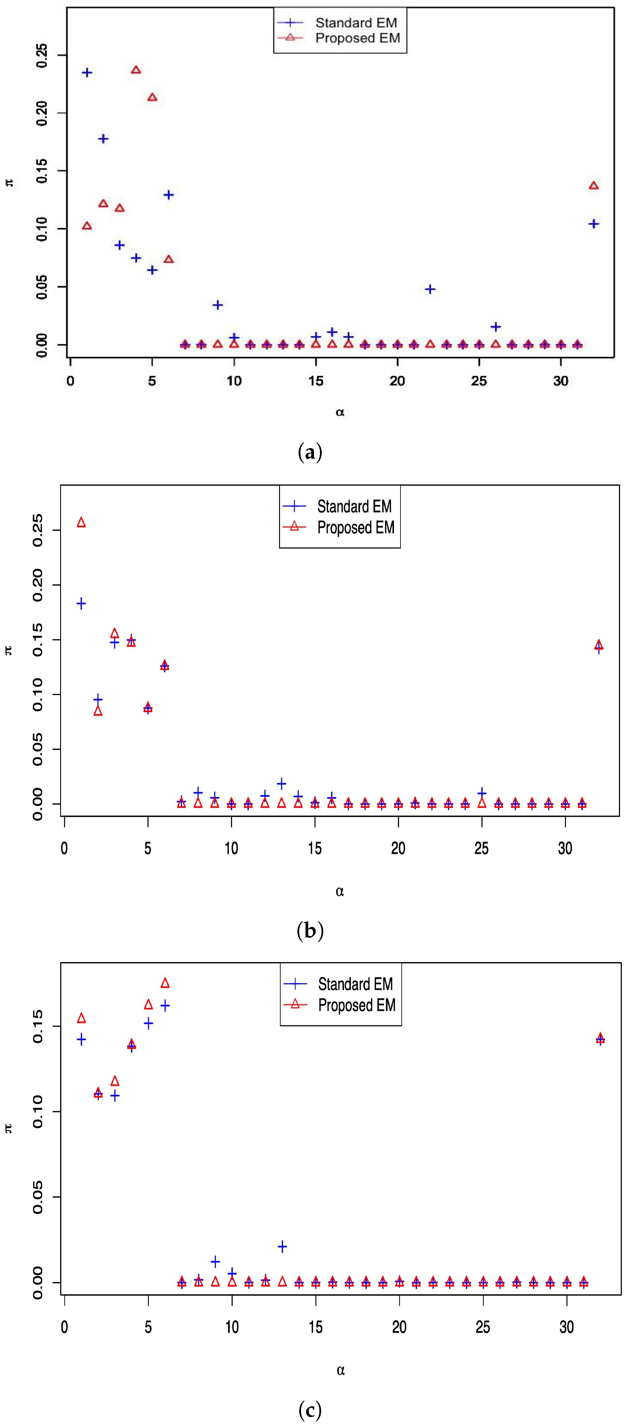
Next, the evaluation is based on Theorem 1 and estimators $\widehat{\mathit{s}}$, $\widehat{\mathit{g}}$, $\widehat{\mathit{F}}$. We note that $-0.19<\frac{-1}{8log2}$ does not satisfy Theorem 1, so the corresponding estimator eliminates many classes. Figure 3 presents the estimated $\widehat{\mathit{F}}$ for different $\lambda$, and we can see that the results of Figure 3a are consistent with the conclusion of Theorem 1. The conclusion is that the $\lambda$s no larger than $-0.19N$ are discarded. In addition, combined with Figure 3a–c, we know that attribute 7 is the most basic attribute. Figure 4a,b display the estimators of guessing and slipping parameters, respectively. According to the estimated $\widehat{\mathit{s}}$, the results of $\lambda =-0.19N$ strongly shifted on items 2, 3, 5, 9, and 16. For different $\lambda$s, the behavior of estimated $\widehat{\mathit{g}}$ is too complex, and significant differences are found in items 8, 9, and 13.

Until now, the candidate penalties are $\lambda =-0.18N$ and $-0.17N$. The penalty $\lambda =-0.17N$ supports the criteria EBIC, and $\lambda =-0.18N$ prefers a simpler model. Furthermore, a denser grid between $[-0.18N,-0.16N]$ will give more detailed results.

6. Discussion

In this paper, we study the penalized method for the DINA model. There are two contributions. Firstly, the entropy penalized method is proposed for the DINA model. The feasible domain is defined to describe the relation between latent classes and the parameter space of item parameters. This framework allows for distinguishing irrelevant attribute profiles. Second, based on the definition of the feasible domain, two modified EM algorithms are developed. In practice, it is recommended to perform exploratory analyses using Algorithm 2 before proceeding further, which can provide valuable insights and guidance to understand the data structure.

While this paper focuses on the DINA model, a natural extension would be the application of the entropy penalized method to other CDMs. Additionally, it is worth noting that this paper study involves situations with a maximum dimension of $K=8$, which is relatively low. In high-dimensional cases of K, improving the power and performance of the entropy-penalized method is an interesting topic. A more challenging question is indicating how the specification of irrelevant latent classes may affect the classification accuracy and the estimation of the model. Those topics are left for future research.

References

1. Junker, B.W.; Sijtsma, K. Cognitive assessment models with few assumptions, and connections with nonparametric item response theory. Appl. Psychol. Meas. 2001, 25, 258–272. [Google Scholar] [CrossRef]
2. Templin, J.L.; Henson, R.A. Measurement of psychological disorders using cognitive diagnosis models. Psychol. Methods 2006, 11, 287–305. [Google Scholar] [CrossRef]
3. Maris, E. Estimating multiple classification latent class models. Psychometrika 1999, 64, 187–212. [Google Scholar] [CrossRef]
4. Hartz, S.M. A Bayesian Framework for the Unified Model for Assessing Cognitive Abilities: Blending Theory with Practicality. Diss. Abstr. Int. B Sci. Eng. 2002, 63, 864. [Google Scholar]
5. DiBello, L.V.; Stout, W.F.; Roussos, L.A. Unified cognitive/psychometric diagnostic assessment likelihood-based classification techniques. In Cognitively Diagnostic Assessment; Routledge: London, UK, 1995; pp. 361–389. [Google Scholar]
6. Henson, R.A.; Templin, J.L.; Willse, J.T. Defining a family of cognitive diagnosis models using log-linear models with latent variables. Psychometrika 2009, 74, 191–210. [Google Scholar] [CrossRef]
7. de la Torre, J. The generalized DINA model framework. Psychometrika 2011, 76, 179–199. [Google Scholar] [CrossRef]
8. von Davier, M. A general diagnostic model applied to language testing data. ETS Res. Rep. Ser. 2005, 2005, i-35. [Google Scholar] [CrossRef]
9. Liu, J.; Xu, G.; Ying, Z. Data-driven learning of Q-matrix. Appl. Psychol. Meas. 2012, 36, 548–564. [Google Scholar] [CrossRef]
10. Chen, Y.; Liu, J.; Xu, G.; Ying, Z. Statistical analysis of Q-matrix based diagnostic classification models. J. Am. Stat. Assoc. 2015, 110, 850–866. [Google Scholar] [CrossRef]
11. Xu, G.; Shang, Z. Identifying latent structures in restricted latent class models. J. Am. Stat. Assoc. 2018, 113, 1284–1295. [Google Scholar] [CrossRef]
12. Gu, Y.; Xu, G. Identification and Estimation of Hierarchical Latent Attribute Models. arXiv 2019, arXiv:1906.07869. [Google Scholar]
13. Gu, Y.; Xu, G. Partial identifiability of restricted latent class models. Ann. Stat. 2020, 48, 2082–2107. [Google Scholar] [CrossRef]
14. Chen, J. Optimal rate of convergence for finite mixture models. Ann. Stat. 1995, 23, 221–233. [Google Scholar] [CrossRef]
15. Gu, Y.; Xu, G. Learning Attribute Patterns in High-Dimensional Structured Latent Attribute Models. J. Mach. Learn. Res. 2019, 20, 1–58. [Google Scholar]
16. Templin, J.; Bradshaw, L. Hierarchical diagnostic classification models: A family of models for estimating and testing attribute hierarchies. Psychometrika 2014, 79, 317–339. [Google Scholar] [CrossRef] [PubMed]
17. Wang, C.; Lu, J. Learning attribute hierarchies from data: Two exploratory approaches. J. Educ. Behav. Stat. 2021, 46, 58–84. [Google Scholar] [CrossRef]
18. Tibshirani, R. Regression shrinkage and selection via the lasso. J. R. Stat. Soc. Ser. B (Methodol.) 1996, 58, 267–288. [Google Scholar] [CrossRef]
19. Zou, H. The adaptive lasso and its oracle properties. J. Am. Stat. Assoc. 2006, 101, 1418–1429. [Google Scholar] [CrossRef]
20. Yuan, M.; Lin, Y. Model selection and estimation in regression with grouped variables. J. R. Stat. Soc. Ser. B (Stat. Methodol.) 2006, 68, 49–67. [Google Scholar] [CrossRef]
21. Fan, J.; Li, R. Variable selection via nonconcave penalized likelihood and its oracle properties. J. Am. Stat. Assoc. 2001, 96, 1348–1360. [Google Scholar] [CrossRef]
22. Ma, J.; Wang, T. Entropy penalized automated model selection on Gaussian mixture. Int. J. Pattern Recognit. Artif. Intell. 2004, 18, 1501–1512. [Google Scholar] [CrossRef]
23. Huang, T.; Peng, H.; Zhang, K. Model selection for Gaussian mixture models. Stat. Sin. 2017, 27, 147–169. [Google Scholar] [CrossRef]
24. de la Torre, J. DINA model and parameter estimation: A didactic. J. Educ. Behav. Stat. 2009, 34, 115–130. [Google Scholar] [CrossRef]
25. Culpepper, S.A. Bayesian estimation of the DINA model with Gibbs sampling. J. Educ. Behav. Stat. 2015, 40, 454–476. [Google Scholar] [CrossRef]
26. Wang, J.; Shi, N.; Zhang, X.; Xu, G. Sequential Gibbs Sampling Algorithm for Cognitive Diagnosis Models with Many Attributes. Multivar. Behav. Res. 2022, 57, 840–858. [Google Scholar] [CrossRef]
27. Shannon, C.E. A mathematical theory of communication. Bell Syst. Tech. J. 1948, 27, 379–423. [Google Scholar] [CrossRef]
28. Thomas, M.; Joy, A.T. Elements of Information Theory; Wiley-Interscience: Hoboken, NJ, USA, 2006. [Google Scholar]
29. Chen, J.; Chen, Z. Extended Bayesian information criteria for model selection with large model spaces. Biometrika 2008, 95, 759–771. [Google Scholar] [CrossRef]
30. Xu, G. Identifiability of restricted latent class models with binary responses. Ann. Stat. 2017, 45, 675–707. [Google Scholar] [CrossRef]
31. Xu, G.; Zhang, S. Identifiability of diagnostic classification models. Psychometrika 2016, 81, 625–649. [Google Scholar] [CrossRef]
32. Tatsuoka, C. Data analytic methods for latent partially ordered classification models. J. R. Stat. Soc. Ser. C (Appl. Stat.) 2002, 51, 337–350. [Google Scholar] [CrossRef]
33. de la Torre, J.; Douglas, J.A. Higher-order latent trait models for cognitive diagnosis. Psychometrika 2004, 69, 333–353. [Google Scholar] [CrossRef]
Figure 1. The results of estimated π ^ for different sample sizes. The horizontal axis represents attribute profiles which can be concluded as 1 ( 0 , 0 , 0 , 0 , 0 ) , 2 ( 1 , 0 , 0 , 0 , 0 ) , 3 ( 0 , 1 , 0 , 0 , 0 ) , …, 7 ( 1 , 1 , 0 , 0 , 0 ) , …, 32 ( 1 , 1 , 1 , 1 , 1 ) . The rules can also apply to different Ks. (a) The results of sample size N = 150 . (b) The results of sample size N = 500 . (c) The results of sample size N = 1000 .
Mathematics 11 03993 g001
Figure 2. Solution paths of the estimated π , the number of F and EBIC versus λ . (a) Solution paths of π . (b) Number of F and EBIC.
Mathematics 11 03993 g002
Figure 3. The estimators of item parameters s and g as the penalty parameter λ varies in the set { 0.19 N , 0.18 N , , 0.15 N } . (a) λ = 0.19 N . (b) λ = 0.18 N . (c) λ = 0.17 N . (d) λ = 0.16 N .
Mathematics 11 03993 g003
Figure 4. The estimators of item parameters s and g as the penalty parameter λ varies in the set { 0.19 N , 0.18 N , , 0.15 N } . (a) Slipping parameters. (b) Guessing parameters.
Mathematics 11 03993 g004