Six-Segment Strategy for Prosumers’ Financial Benefit Maximization in Local Peer-to-Peer Energy Trading

Abstract

The notion of prosumers, people who create and consume energy, has emerged in the energy sector as a result of the fast integration of renewable energy sources and advances in digital technology. Platforms for peer-to-peer (P2P) energy trading have come to light as viable ways to allow prosumers to conduct direct energy transactions within small groups. Existing P2P trading models, however, frequently lack an optimized approach to maximize the advantages for prosumers. In this article, we provide a novel six-segment strategy (SSS) that is intended to increase prosumers′ ability to maximize their benefits in P2P energy trading systems. Additionally, the SSS promotes prosumers′ active market engagement by supporting community-driven energy exchanges. Through extensive mathematical modeling, simulations, and case studies, we demonstrate the effectiveness of the six-segment strategy in enhancing the economic benefits of prosumers participating in P2P energy trading. The proposed optimization strategy holds the potential to revolutionize the energy landscape by promoting more sustainable and consumer-centric energy trading. The cost savings of 12.9% are distributed among prosumers by the SSS, which is an improvement compared with previously proposed strategies.

1. Introduction

The modern energy landscape is witnessing a transformative shift with the proliferation of renewable energy sources and the emergence of prosumers, individuals who actively participate both as energy consumers and producers within the energy grid. This paradigm shift has led to the development of innovative energy trading platforms, known as peer-to-peer (P2P) energy trading systems, which enable prosumers to engage in direct energy exchanges within localized communities, e.g., the local electricity market (LEM) [1]. By facilitating efficient energy transactions, P2P energy trading holds the promise of revolutionizing traditional energy markets and empowering consumers to play an active role in shaping the energy ecosystem [2].

Despite the potential benefits, current P2P energy trading models often lack a comprehensive strategy to maximize the advantages for prosumers involved in the system. Consequently, prosumers may face challenges in optimizing their energy consumption and generation patterns to reap the full economic potential of their participation [3]. An investigation [4] presented strong evidence regarding the financial advantages for peers who share energy at the local level in a small energy community. To significantly increase consumer partaking, it is essential for flexible market operations and techniques to align with customers′ preferences. To understand customers′ motivations, such as self-reliance and monetary rewards, a customer-centric approach is necessary [5] to effectively engage them [6]. The research in [7] suggested a commitment system based on smart contracts and a trusted execution environment to address the trust issue among market players because the distributed energy trading model lacks an efficient trust strategy. To mention an important dimension of energy storage, the suggested strategy in [8] illustrates the potential of energy storage as an efficient tool for managing congestion and operating cost optimization in distribution networks by offering financial advantages to both the microgrid and the distribution system operator through thorough simulations and analyses. The research in [9] suggested a method for taking the solution to the next level, in which nearby microgrids in a distribution network cooperate and create a multi-microgrid to construct a shared energy storage to boost their revenue and raise their dependability. The annual compensation received from system operators is taken into account while comparing various investment possibilities. Operators award annual rewards depending on the contribution of energy storage to peak-shaving and annual cost savings in distribution network operation for each of the investment scenarios.

Increasing the earnings that prosumers may make by reselling this surplus into the neighborhood network is one strategy to expand the number of prosumers. Additionally, customers would benefit from cheaper pricing as a consequence of competition among prosumers, paying less for power that is not subject to network charges. The use of P2P contracts negotiated in local marketplaces and operated at the microgrid stage serves as a method of facilitating this kind of transaction [10]. One study [11] introduced a novel marketplace for prosumers’ energy surplus trading in a genuine local microgrid based on intelligent P2P contracts. The study outlined in reference [12] introduced a pair of bidding approaches intended for the P2P market. It scrutinized the impact of these strategies on augmenting liquidity, stabilizing prices, and achieving profitability. The investigation drew upon historical data from a previous demonstration project concerning solar PV generation and consumption. The research in [13] demonstrated that providing fiscal incentives encourages prosumers to finance in or improvement to energy-efficient resources. Consequently, there is a need for comprehensive strategies to engage customers [14,15], empowering them to utilize their resources effectively. Our research goal statement revolves around this premise.

2. Related Work and Background

To address this critical gap, in our previous work [16], we proposed a novel and holistic approach to prosumer segmentation, which aims to enhance prosumers′ benefit maximization in local energy trading. In prior research, our work has delved into the design and optimization of LEM, with a particular focus on enhancing prosumer engagement and financial incentives. We introduced a distinctive two-stage optimization approach within the LEM framework, aiming to achieve two critical objectives: system cost reduction and the maximization of monetary rewards for prosumers. The first stage of our proposed approach concentrates on minimizing system costs. To facilitate this, we introduced an innovative tactic involving customer segmentation [17]. This segmentation is based on optimized power export, a key outcome of the initial optimization stage. By categorizing prosumers according to their power export optimization, we aimed to create a more targeted and effective approach to reward maximization in the subsequent stages. In addition, we presented four distinct strategies for calculating monetary rewards for prosumers within the LEM. Notably, two of these strategies take into account the prosumer segments established in the first stage of our optimization approach, thereby aligning the monetary reward calculation with the individual characteristics and behaviors of prosumers. This background information provides essential context for our current research, which builds upon these foundations to explore further advancements in LEM optimization and prosumer engagement. Our updated results and findings are presented in the subsequent sections of this paper, offering insights into the ongoing evolution of LEM design and its impact on prosumer participation and financial incentives. In the present work, we propose six segments and new reward limits, which show enhanced results compared with three-segment strategies.

The innovation and major contribution of our study are outlined as follows:

• A mathematical model of P2P energy trading in the local community is proposed to optimize the system cost and revenue of prosumers;
• Novel prosumer segmentation rules and reward limits were designed on the basis of peak and average power export, which resulted after the first phase of optimization;
• A second stage of optimization was implemented for prosumers’ reward maximization;
• The final results of six-segment strategies (SSSs) were compared with the three-segment results.

We propose our P2P model in Section 3. The mathematical representation of the model is explained in Section 4. Section 5 describes the numerical values of all model parameters. The results are analyzed in Section 6, and the work is concluded in Section 7.

3. Proposed P2P Model

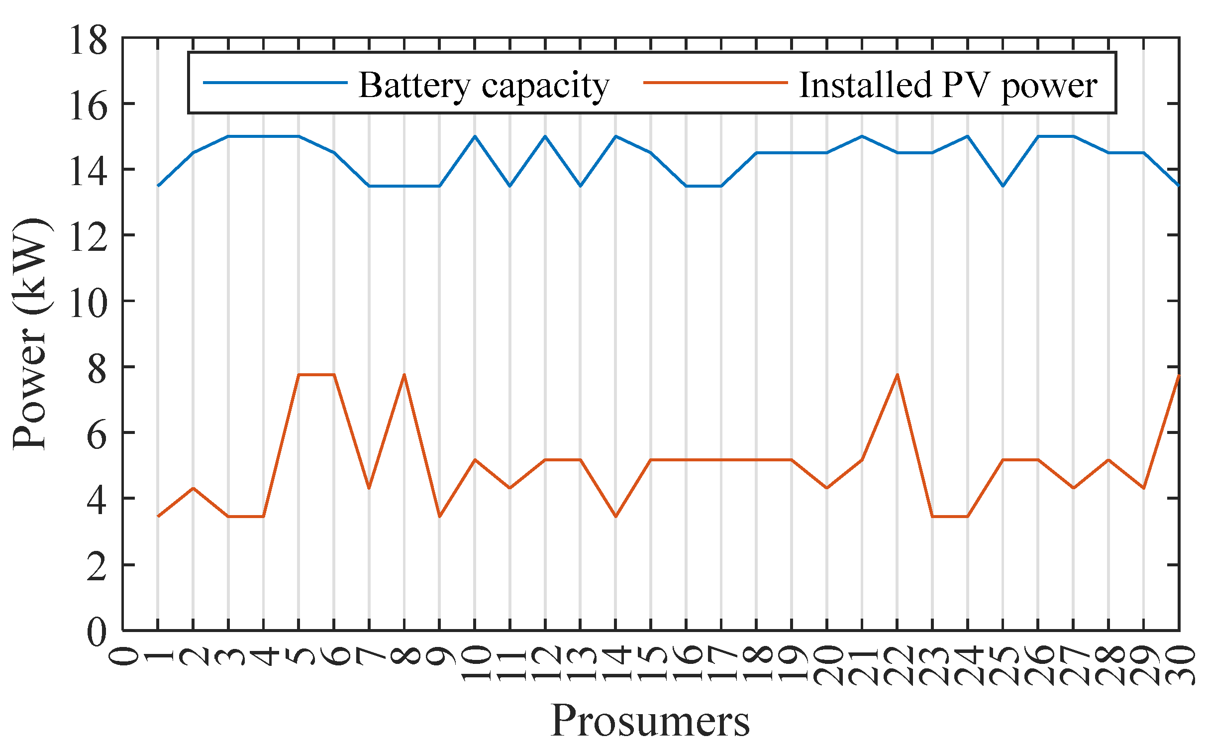
In this research, we conducted simulations on a local energy network comprising 36 households, 30 of which were prosumers equipped with solar PV and battery backup, enabling them to engage in P2P energy trading. The remaining six customers were normal consumers restricted to importing power without generating or selling it. The primary focus was on calculating the power transaction cost for two distinct cases: one without P2P and another with P2P implementation.

There were two cases considered for the study, as shown in

Table 1. Cases considered for study.

Cases	Strategy	Financial Incentive	Incentive Function
Case 01 Without P2P	-	×	-
Case 02 With P2P	01	✓	Identical to all
	02	✓	40% of revenue
	03	✓	Peak power export
	04	✓	Avg power export

, which includes the SSS. For Case 1, electricity transactions were solely permitted with the grid, enabling customers to purchase the power at retail prices and prosumers to sell excess power to the utility grid at feed-in prices. In Case 2, besides the utility grid power exchange, customers were also allowed to buy energy from the peer prosumer at the P2P price or mid-market price, as specified by Equation (19). Additionally, prosumers in Case 2 had the option to trade electricity to other peers at P2P price or to the utility grid at feed-in prices.

The motivation behind these strategies is to address customers′ growing demand for rate alternatives that can help reduce their electricity bills. Strategies 3 and 4 aim to classify customers by providing monetary rewards depending on their power export. In Strategy 3, classification is founded on the highest exported power, while Strategy 4 classifies prosumers by their average exported power. This approach encourages prosumers to strive for higher rewards, motivating them to improve their power export performance. However, it is essential to ensure that the sum of rewards provided to all prosumers collectively remains under the cost-saving threshold. The detailed segment rules and incentive limits are detailed in

Table 2. Segment rules and incentive limit.

Segment	Strategy 3		Strategy 4
	Peak Power Export (kW)	Incentive Limit (% of Max Reward)	Average Power Export (kW)	Incentive Limit (% of Max Reward)
S1	0–1	50%	0–0.1	25%
S2	1–2	60%	0.1–0.15	50%
S3	2–3	75%	0.15–0.2	70%
S4	3–4	100%	0.2–0.25	90%
S5	4–5	130%	0.25–0.3	120%
S6	>5	160%	>0.3	150%

.

Overall, these strategies and the implementation of P2P hold promise for enhancing cost savings and incentivizing prosumers to actively participate in the energy market, contributing to a more sustainable and efficient energy exchange.

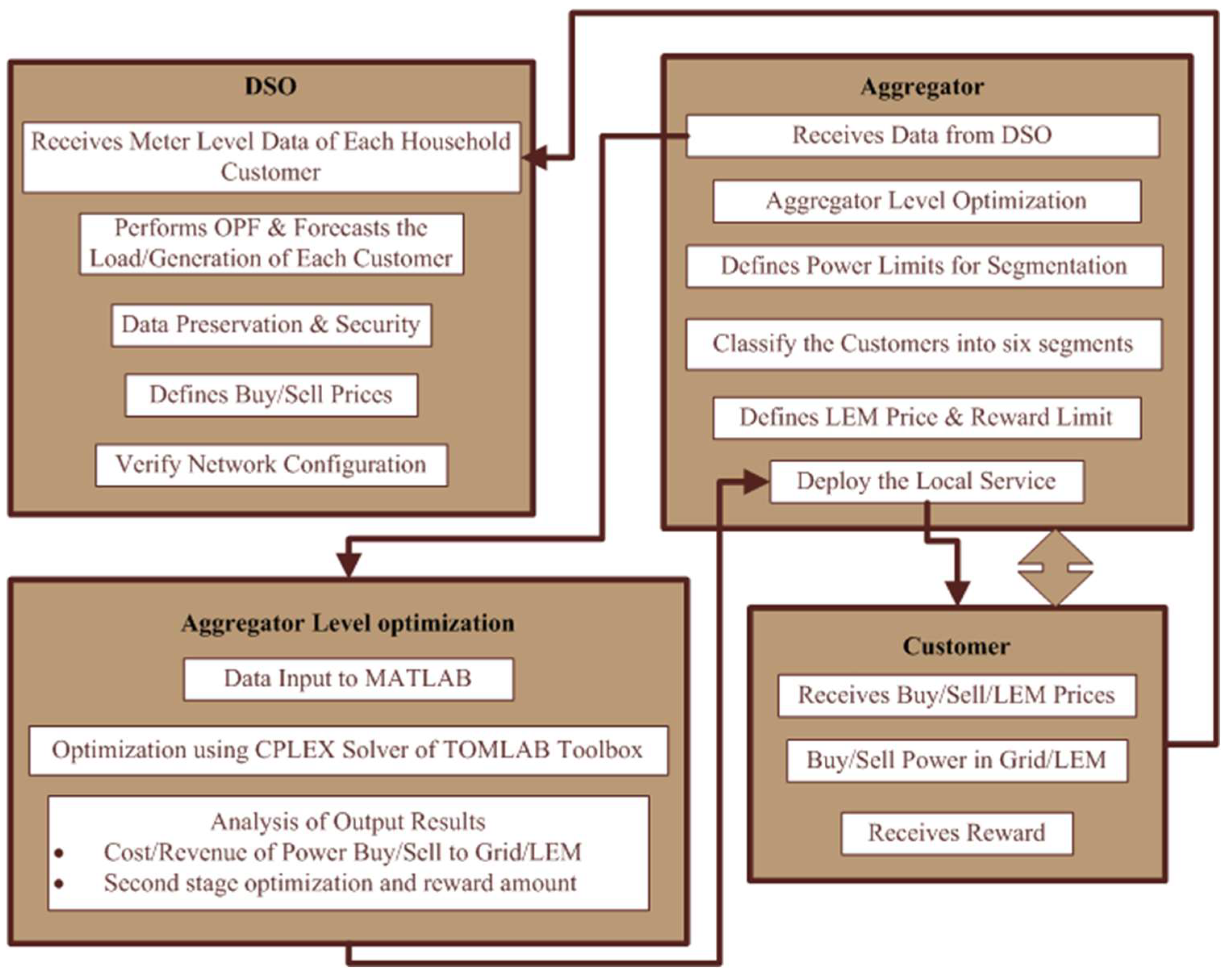
The step-by-step methodology of market operation is illustrated in Figure 1, outlining the roles and responsibilities of the distribution system operator (DSO), the aggregator, and the participants, as well as their interrelationships. The optimization process conducted in this study is specifically focused on the aggregator level. In this context, the aggregator assumes control over the community and presents an optimal operation solution, factoring in the objective function. On the other hand, the DSO is responsible for receiving and preserving the smart meter data of customers to run optimal power flow (OPF). The DSO defines the power exchange prices and the network configuration. It is important to note that market clearing is not pursued in this scenario, as the aggregator is responsible for proposing and implementing the most advantageous transaction arrangement within the community.

4. Mathematical Model

The primary goal of the initial optimization stage is to formulate the objective function in a way that minimizes the overall system cost, as described by Equation (1).

$$\mathrm{Min}\left(\sum _{\mathsf{\tau }=1}^{{\mathrm{N}}_{\mathsf{\tau }}}\sum _{\mathrm{j}=1}^{{\mathrm{N}}_{\mathrm{j}}}\left({\mathrm{Q}}_{j,\tau }^{\mathrm{g}}-{\mathrm{R}}_{j,\tau }^{\mathrm{g}}\right)+{(\mathrm{Q}}_{j,\tau }^{\mathrm{p}2\mathrm{p}}-{\mathrm{R}}_{j,\tau }^{\mathrm{p}2\mathrm{p}})+{\mathrm{Z}}_{\mathrm{j},\mathsf{\tau }}\right)$$

(1)

In this context, ${\mathrm{Q}}_{j,\tau }^g$ and ${\mathrm{R}}_{j,\tau }^g$ denote the cost and income, respectively, for prosumers interacting with the grid. On the other hand, ${\mathrm{Q}}_{j,\tau }^{p2p}$ and ${\mathrm{R}}_{j,\tau }^{p2p}$ represent the cost and income, respectively, for prosumers engaged in energy sharing with peers locally. Additionally, ${\mathrm{Z}}_{j,\tau }$ signifies the fixed charge applicable to each prosumer.

$${\mathrm{Q}}_{j,\tau }^g=\left( {\mathrm{Ƥ}}_{j,\tau }^b\times {\mathrm{Л}}_{j,\tau }^b\right)\times d\tau \hspace{1em}{\forall j\in \mathrm{N}}_j , {\forall \tau \in \mathrm{N}}_{\tau }$$

(2)

$${\mathrm{R}}_{j,\tau }^g=({\mathrm{Ƥ}}_{j,\tau }^s\times {\mathrm{Л}}_{j,\tau }^f)\times d\tau \hspace{1em}{\forall j\in \mathrm{N}}_j , {\forall \tau \in \mathrm{N}}_{\tau }$$

(3)

Expressions (2) and (3) outline the mathematical computations for determining the cost and revenue associated with power interchange to the grid for all prosumers, subject to constrictions (4–7). In these equations, ${\mathrm{Ƥ}}_{j,\tau }^b$ and ${\mathrm{Ƥ}}_{j,\tau }^s$ represent the power purchased from and sold to the grid, respectively. ${\mathrm{Л}}_{j,\tau }^b$ and ${\mathrm{Л}}_{j,\tau }^f$ represent the power exchange rates for buy and sell, respectively, while d$\tau$ serves as the time period adjustment factor

$$0 \le {\mathrm{Ƥ}}_{j,t}^b\le {\mathrm{Ƥ}}_{j,\tau }^{b max}\times {\mathsf{\beta }}_{j,\tau }^{\mathrm{Ƥ}\mathrm{b}} {\forall j\in \mathrm{N}}_j , {\forall \tau \in \mathrm{N}}_{\tau }$$

(4)

$$0\le {\mathrm{Ƥ}}_{j,\tau }^s \le {\mathrm{Ƥ}}_{j,\tau }^{s max}\times {\mathsf{\beta }}_{j,\tau }^{\mathrm{Ƥ}\mathrm{s}} {\forall j\in \mathrm{N}}_j , {\forall \tau \in \mathrm{N}}_{\tau }$$

(5)

In this context, Equations (4) and (5) establish the boundaries for power trading, with ${\mathrm{Ƥ}}_{j,\tau }^{b max}$ representing the maximum allowable power purchase and ${\mathrm{Ƥ}}_{j,\tau }^{s max}$ indicating the maximum permissible power sell. Their corresponding binary variables are symbolized as ${\mathsf{\beta }}_{j,\tau }^{\mathrm{Ƥ}\mathrm{b}}$ and ${\mathsf{\beta }}_{j,\tau }^{\mathrm{Ƥ}\mathrm{s}}$. These variables are used to express whether a prosumer engages in power purchase or power sell transactions.

$$0\le {\mathsf{\beta }}_{j,\tau }^{\mathrm{Ƥ}\mathrm{b}}\le 1 {\forall j\in \mathrm{N}}_j , {\forall \tau \in \mathrm{N}}_{\tau }$$

(6)

$$0\le {\mathsf{\beta }}_{j,\tau }^{\mathrm{Ƥ}\mathrm{s}} \le 1 {\forall j\in \mathrm{N}}_j , {\forall \tau \in \mathrm{N}}_{\tau }$$

(7)

$${\mathsf{\beta }}_{j,\tau }^{\mathrm{Ƥ}\mathrm{b}}+{\mathsf{\beta }}_{j,\tau }^{\mathrm{Ƥ}\mathrm{s}}\le 1 {\forall j\in \mathrm{N}}_j , {\forall \tau \in \mathrm{N}}_{\tau }$$

(8)

The limitations on the binary variables are defined in Equations (6) and (7). Constraint (8) ensures that a prosumer cannot perform both power buying and selling operations with the grid simultaneously.

Equations (9) and (10) are the mathematical representations for assessing the cost and revenue associated with electricity buy and sell transactions in P2P for all prosumers. These calculations are subject to limits (11–18).

$${\mathrm{Q}}_{j,\tau }^{\mathrm{p}2\mathrm{p}}=\left(l_{p2p}^{buy}\times {\mathrm{Ƥ}}_{j,\tau }^{b \mathrm{p}2\mathrm{p}}\times {\mathrm{Л}}_{j,\tau }^{\mathrm{p}2\mathrm{p}}\right)\times d\tau {\forall j\in \mathrm{N}}_j$$

(9)

$${\mathrm{R}}_{j,\tau }^{\mathrm{p}2\mathrm{p}}=\left(l_{p2p}^{sell}\times {\mathrm{Ƥ}}_{j,\tau }^{s \mathrm{p}2\mathrm{p}}\times {\mathrm{Л}}_{j,\tau }^{\mathrm{p}2\mathrm{p}}\right)\times d\tau {\forall j\in \mathrm{N}}_j$$

(10)

where ${\mathrm{Ƥ}}_{j,\tau }^{b \mathrm{p}2\mathrm{p}}$ and ${\mathrm{Ƥ}}_{j,\tau }^{s \mathrm{p}2\mathrm{p}}$ represent the power purchased and sold in P2P, respectively, while ${\mathrm{Л}}_{j,\tau }^{\mathrm{p}2\mathrm{p}}$ denotes the P2P price applicable to all participants. Within the P2P framework, the prosumers may take into account network losses as a central factor during the process of matching peers [18]. The power loss coefficients for power buying and selling in P2P are denoted as $l_{p2p}^{buy}$ and $l_{p2p}^{sell}$, respectively. The overall power loss multiplier for energy transactions in the local energy trading is fixed at 5% [19].

$$0\le {\mathrm{Ƥ}}_{j,\tau }^{b \mathrm{p}2\mathrm{p}} \le {\mathrm{Ƥ}}_{j,\tau }^{b max}\times {\mathsf{\beta }}_{j,\tau }^{\mathrm{Ƥ}\mathrm{b}\mathrm{p}2\mathrm{p}}\hspace{1em}{\forall j\in \mathrm{N}}_j , {\forall \tau \in \mathrm{N}}_{\tau }$$

(11)

$$0\le {\mathrm{Ƥ}}_{j,\tau }^{s \mathrm{p}2\mathrm{p}} \le {\mathrm{Ƥ}}_{j,\tau }^{s max}\times {\mathsf{\beta }}_{j,\tau }^{\mathrm{Ƥ}\mathrm{s}\mathrm{p}2\mathrm{p}}\hspace{1em}{\forall j\in \mathrm{N}}_j , {\forall \tau \in \mathrm{N}}_{\tau }$$

(12)

Here, constraints (11) and (12) define the limitations for power trading among peers at the local level. The binary variables ${\mathsf{\beta }}_{j,\tau }^{\mathrm{Ƥ}\mathrm{b}\mathrm{p}2\mathrm{p}}$ and ${\mathsf{\beta }}_{j,\tau }^{\mathrm{Ƥ}\mathrm{s}\mathrm{p}2\mathrm{p}}$ are used to express whether a prosumer engages in power purchase or power sell transactions in P2P, respectively. These variables help establish the boundaries for the power buy and sell operations within P2P.

$$0\le {\mathsf{\beta }}_{j,\tau }^{\mathrm{Ƥ}\mathrm{b}\mathrm{p}2\mathrm{p}}\le 1 {\forall j\in \mathrm{N}}_j , {\forall \tau \in \mathrm{N}}_{\tau }$$

(13)

$$0\le {\mathsf{\beta }}_{j,\tau }^{\mathrm{Ƥ}\mathrm{s}\mathrm{p}2\mathrm{p}}\le 1 {\forall j\in \mathrm{N}}_j , {\forall \tau \in \mathrm{N}}_{\tau }$$

(14)

$${\mathsf{\beta }}_{j,\tau }^{\mathrm{Ƥ}\mathrm{b}\mathrm{p}2\mathrm{p}}+{\mathsf{\beta }}_{j,\tau }^{\mathrm{Ƥ}\mathrm{s}\mathrm{p}2\mathrm{p}}\le 1 {\forall j\in \mathrm{N}}_j , {\forall \tau \in \mathrm{N}}_{\tau }$$

(15)

$${\mathsf{\beta }}_{j,\tau }^{\mathrm{Ƥ}\mathrm{b}}+{\mathsf{\beta }}_{j,\tau }^{\mathrm{Ƥ}\mathrm{s}\mathrm{p}2\mathrm{p}}\le 1 {\forall j\in \mathrm{N}}_j , {\forall \tau \in \mathrm{N}}_{\tau }$$

(16)

$${\mathsf{\beta }}_{j,\tau }^{\mathrm{Ƥ}\mathrm{b}\mathrm{p}2\mathrm{p}}+{\mathsf{\beta }}_{j,\tau }^{\mathrm{Ƥ}\mathrm{s}}\le 1 {\forall j\in \mathrm{N}}_j , {\forall \tau \in \mathrm{N}}_{\tau }$$

(17)

$$\sum _{j=1}^{N_j}{\mathrm{Ƥ}}_{j,\tau }^{b \mathrm{p}2\mathrm{p}}= \sum _{j=1}^{N_j}{\mathrm{Ƥ}}_{j,\tau }^{s \mathrm{p}2\mathrm{p}}{\forall j\in \mathrm{N}}_j , {\forall \tau \in \mathrm{N}}_{\tau }$$

(18)

where a restriction defined by Equations (13) and (14) on the binary variables influences the actions of prosumers within P2P. Specifically, it enforces that prosumers can choose either to purchase or to sell power in P2P, but not both simultaneously.

Constraints (15)–(17) prevent a participant from engaging in simultaneous operations both in the grid and the P2P, while expression (18) signifies equilibrium between power transactions in the P2P transaction. In other words, during time period $\tau$, a prosumer can either trade power with the grid or participate in P2P, but not both. The P2P price is determined on the basis of Equation (19) and is computed as an average of the smallest purchase price of each household and the feed-in price [20].

$${\mathrm{Л}}_{j,\tau }^{\mathrm{p}2\mathrm{p}}=\frac{\mathrm{m}\mathrm{i}\mathrm{n}\left({\mathrm{Л}}_{j,\tau }^b\right)+{\mathrm{Л}}_{j,\tau }^f}{2} {\forall j\in \mathrm{N}}_j, {\forall \tau \in \mathrm{N}}_{\tau }$$

(19)

Equations (20) and (21) illustrate the mathematical model for the batteries of the players. The mathematical representation of the first charging power is calculated by Equation (20), while for all other times, Equation (21) is used:

$${\mathrm{Ƥ}}_{j,1}^{bat}={\mathrm{Ƥ}}_{j,ini}^{bat}+{\mathrm{Ƥ}}_{j,1}^{ch}\times {\mathsf{\eta }}_{j,ch}-\frac{{\mathrm{Ƥ}}_{j,1}^{dch}}{{\mathsf{\eta }}_{j,dch}}{\forall h\in \mathrm{N}}_h$$

(20)

$${\mathrm{Ƥ}}_{j,\tau }^{bat}={\mathrm{Ƥ}}_{j,\tau -1}^{bat}+{\mathrm{Ƥ}}_{j,\tau }^{ch}\times {\mathsf{\eta }}_{j,ch}-\frac{{\mathrm{Ƥ}}_{j,\tau }^{dch}}{{\mathsf{\eta }}_{j,dch}} {\forall j\in \mathrm{N}}_j,{\forall \tau \in [2,\mathrm{N}}_{\tau }]$$

(21)

where ${\mathrm{Ƥ}}_{j,\tau }^{bat}$ characterizes the battery power, and charge and discharge efficiencies are symbolized as ${\mathsf{\eta }}_{j,ch}$ and ${\mathsf{\eta }}_{j,dch}$. Expression (21) governs the battery charging process throughout all time periods. These energy balance equations are constrained by conditions (19)–(21).

$${0\le \mathrm{Ƥ}}_{j,\tau }^{bat}\le {\mathrm{Ƥ}}_{j,\tau }^{bat max} {\forall j\in \mathrm{N}}_j , {\forall \tau \in \mathrm{N}}_{\tau }$$

(22)

$${0\le \mathrm{Ƥ}}_{j,\tau }^{ch}\le {\mathrm{Ƥ}}_{j,\tau }^{bcl}\times {{\mathsf{\beta }}_{\mathrm{Ƥ}}}_{j,\tau }^{ch} {\forall j\in \mathrm{N}}_j , {\forall \tau \in \mathrm{N}}_{\tau }$$

(23)

$$0\le {\mathrm{Ƥ}}_{j,\tau }^{dch} \le {\mathrm{Ƥ}}_{j,\tau }^{bdl}\times {{\mathsf{\beta }}_{\mathrm{Ƥ}}}_{j,\tau }^{dch} {\forall j\in \mathrm{N}}_j , {\forall \tau \in \mathrm{N}}_{\tau }$$

(24)

Equation (22) pertains to the battery capacity ${\mathrm{Ƥ}}_{j,\tau }^{bat}$ and the upper limit of power in the battery ${\mathrm{Ƥ}}_{j,\tau }^{batmax}$. Meanwhile, constraints (23) and (24) impose limitations on the charging and discharging of the battery, ensuring they remain within specific boundaries. In these constraints, ${\mathrm{Ƥ}}_{j,\tau }^{ch}$ and ${\mathrm{Ƥ}}_{j,\tau }^{dch}$ denote the charging and discharging power, respectively, and ${{\mathsf{\beta }}_{\mathrm{Ƥ}}}_{j,\tau }^{ch}$ & ${{\mathsf{\beta }}_{\mathrm{Ƥ}}}_{j,\tau }^{dch}$ are their corresponding binary variables. Furthermore, ${\mathrm{Ƥ}}_{j,\tau }^{bcl}$ and ${\mathrm{Ƥ}}_{j,\tau }^{bdl}$ represent the power limits for charging and discharging, respectively.

$$0\le {{\mathsf{\beta }}_{\mathrm{Ƥ}}}_{j,\tau }^{ch}\le 1 {\forall j\in \mathrm{N}}_j , {\forall \tau \in \mathrm{N}}_{\tau }$$

(25)

$$0\le {{\mathsf{\beta }}_{\mathrm{Ƥ}}}_{j,\tau }^{dch}\le 1 {\forall j\in \mathrm{N}}_j , {\forall \tau \in \mathrm{N}}_{\tau }$$

(26)

$${{\mathsf{\beta }}_{\mathrm{Ƥ}}}_{j,\tau }^{ch}+{{\mathsf{\beta }}_{\mathrm{Ƥ}}}_{j,\tau }^{dch}=1 {\forall j\in \mathrm{N}}_j , {\forall \tau \in \mathrm{N}}_{\tau }$$

(27)

The binary variables ${{\mathsf{\beta }}_{\mathrm{Ƥ}}}_{j,\tau }^{ch}$ and ${{\mathsf{\beta }}_{\mathrm{Ƥ}}}_{j,\tau }^{dch}$ are constrained by (25) and (26). Constraint (27) ensures that the battery cannot be simultaneously charged and discharged, limiting it to either charging or discharging at any given time.

To enhance the realism of the mathematical model, additional constraints (28)–(30) are incorporated. Equation (28) represents the power balance equation, applied individually to each player in each time period.

$${\mathrm{Ƥ}}_{j,\tau }^l+{\mathrm{Ƥ}}_{j,\tau }^{exp}+{\mathrm{Ƥ}}_{j,\tau }^{ch}={\mathrm{Ƥ}}_{j,\tau }^{imp}+{\mathrm{Ƥ}}_{j,\tau }^{dch}+{\mathrm{Ƥ}}_{j,\tau }^{gen} {\forall j\in \mathrm{N}}_j,{\forall \tau \in \mathrm{N}}_{\tau }$$

(28)

$${\mathrm{Ƥ}}_{j,\tau }^{imp}={\mathrm{Ƥ}}_{j,\tau }^b+{\mathrm{Ƥ}}_{j,\tau }^{b\mathrm{p}2\mathrm{p}} {\forall j\in \mathrm{N}}_j,{\forall \tau \in \mathrm{N}}_{\tau }$$

(29)

$${\mathrm{Ƥ}}_{j,\tau }^{exp}={\mathrm{Ƥ}}_{j,\tau }^s+{\mathrm{Ƥ}}_{j,\tau }^{s\mathrm{p}2\mathrm{p}} {\forall j\in \mathrm{N}}_j,{\forall \tau \in \mathrm{N}}_{\tau }$$

(30)

where ${\mathrm{Ƥ}}_{j,\tau }^{imp}$ is imported power, ${\mathrm{Ƥ}}_{j,\tau }^{dch}$ is the power discharged from battery, ${\mathrm{Ƥ}}_{j,\tau }^{gen}$ is power generation, ${\mathrm{Ƥ}}_{j,\tau }^l$ is power consumed by load, ${\mathrm{Ƥ}}_{j,\tau }^{exp}$ is power exported, ${\mathrm{Ƥ}}_{j,\tau }^{ch}$ is power charged in the battery. Equation (29) calculates the imported power. On the other hand, Equation (30) computes the exported power.

The second phase of optimization is described below, which is the mathematical model of the SSS.

$$\mathrm{Max}\left(\sum _{\tau =1}^{N_{\tau }}\sum _{j=1}^{N_j}\left({\mathrm{R}}_{j,\tau }^{S1}+{\mathrm{R}}_{j,\tau }^{S2}+{\mathrm{R}}_{j,\tau }^{S3}+{\mathrm{R}}_{j,\tau }^{S4}+{\mathrm{R}}_{j,\tau }^{S5}+{\mathrm{R}}_{j,\tau }^{S6}\right)\right)$$

(31)

Equation (30) is the mathematical representation of the objective function of second-phase optimization to maximize the overall financial reward received by prosumers, where ${\mathrm{R}}_{j,\tau }^{S1}$, ${\mathrm{R}}_{j,\tau }^{S2}$, ${\mathrm{R}}_{j,\tau }^{S3}$, ${\mathrm{R}}_{j,\tau }^{S4}$, ${\mathrm{R}}_{j,\tau }^{S5}$, and ${\mathrm{R}}_{j,\tau }^{S6}$ are the monetary incentives for prosumers under the six segments S1, S2, S3, S4, S5, and S6 respectively.

$${0\le \mathrm{Ƥ}\mathrm{E}}_{peak}^{S1}<1$$

(32)

$${1\le \mathrm{Ƥ}\mathrm{E}}_{peak}^{S2}<2$$

(33)

$${2\le \mathrm{Ƥ}\mathrm{E}}_{peak}^{S3}<3$$

(34)

$${3\le \mathrm{Ƥ}\mathrm{E}}_{peak}^{S4}<4$$

(35)

$${4\le \mathrm{Ƥ}\mathrm{E}}_{peak}^{S5}<5$$

(36)

$${\mathrm{Ƥ}\mathrm{E}}_{peak}^{S6}\ge 5$$

(37)

$${0\le \mathrm{Ƥ}\mathrm{E}}_{avg}^{S1}<0.1$$

(38)

$${0.1\le \mathrm{Ƥ}\mathrm{E}}_{avg}^{S2}<0.15$$

(39)

$${0.15\le \mathrm{Ƥ}\mathrm{E}}_{avg}^{S3}<0.2$$

(40)

$${0.2\le \mathrm{Ƥ}\mathrm{E}}_{avg}^{S4}<0.25$$

(41)

$${0.25\le \mathrm{Ƥ}\mathrm{E}}_{avg}^{S5}<0.3$$

(42)

$${\mathrm{Ƥ}\mathrm{E}}_{avg}^{S6}\ge 0.3$$

(43)

The range of the maximum and minimum peak power export values for the six segments of prosumers can be found using Equations (32)–(37) in Strategy 3. Likewise, the higher and lower bounds for the average exported power values for the segments can be determined using Equations (38)–(43) in Strategy 4. These equations provide the limits for peak power export, ${\mathrm{Ƥ}\mathrm{E}}_{peak}^{S1}$, ${\mathrm{Ƥ}\mathrm{E}}_{peak}^{S2}$, ${\mathrm{Ƥ}\mathrm{E}}_{peak}^{S3}{,\mathrm{Ƥ}\mathrm{E}}_{peak}^{S4}$, ${\mathrm{Ƥ}\mathrm{E}}_{peak}^{S5}$, and ${\mathrm{Ƥ}\mathrm{E}}_{peak}^{S6}$, as well as average power export, ${\mathrm{Ƥ}\mathrm{E}}_{avg}^{S1}$, ${\mathrm{Ƥ}\mathrm{E}}_{avg}^{S2}$, ${\mathrm{Ƥ}\mathrm{E}}_{avg,}^{S3}{\mathrm{Ƥ}\mathrm{E}}_{avg}^{S4}$, ${\mathrm{Ƥ}\mathrm{E}}_{avg}^{S5}$ and ${\mathrm{Ƥ}\mathrm{E}}_{avg}^{S6}$. It is important to note that these power export values, whether peak or average, are not variable entities; instead, they are derived from the optimized power value ${\mathrm{Ƥ}}_{j,\tau }^{exp}$ obtained during the initial optimization phase. This information is further detailed in Table 2 and mathematical representations (32)–(43).

$$R^{min}=0$$

(44)

$$R^{max}=\frac{D}{{\mathrm{N}}_j} {\forall j\in \mathrm{N}}_j$$

(45)

The lower limit for the incentive amount $R^{min}$ and the upper limit $R^{max}$ are constrained according to Equations (44) and (45), where $D$ is the cost savings. These equations involve the cost savings, which signifies the disparity in savings achieved when comparing scenarios without and with P2P.

$$0<{\mathrm{R}}_{j,\tau }^{S1}\le {\mathsf{\Phi }}_{j,\tau }^{S1}\times R^{max}\times {\mathsf{\beta }}_{{\mathrm{R}}_{j,\tau }^{S1}} \forall j\in {\mathrm{N}}_j , {\forall \tau \in \mathrm{N}}_{\tau }$$

(46)

$$0<{\mathrm{R}}_{j,\tau }^{S2}\le {\mathsf{\Phi }}_{j,\tau }^{S2}\times R^{max}\times {\mathsf{\beta }}_{{\mathrm{R}}_{j,\tau }^{S2}} \forall j\in {\mathrm{N}}_j , {\forall \tau \in \mathrm{N}}_{\tau }$$

(47)

$$0<{\mathrm{R}}_{j,\tau }^{S3}\le {\mathsf{\Phi }}_{j,\tau }^{S3}\times R^{max}\times {\mathsf{\beta }}_{{\mathrm{R}}_{j,\tau }^{S3}} \forall j\in {\mathrm{N}}_j , {\forall \tau \in \mathrm{N}}_{\tau }$$

(48)

$$0<{\mathrm{R}}_{j,\tau }^{S4}\le {\mathsf{\Phi }}_{j,\tau }^{S4}\times R^{max}\times {\mathsf{\beta }}_{{\mathrm{R}}_{j,\tau }^{S4}} \forall j\in {\mathrm{N}}_j , {\forall \tau \in \mathrm{N}}_{\tau }$$

(49)

$$0<{\mathrm{R}}_{j,\tau }^{S5}\le {\mathsf{\Phi }}_{j,\tau }^{S5}\times R^{max}\times {\mathsf{\beta }}_{{\mathrm{R}}_{j,\tau }^{S5}} \forall j\in {\mathrm{N}}_j , {\forall \tau \in \mathrm{N}}_{\tau }$$

(50)

$$0<{\mathrm{R}}_{j,\tau }^{S6}\le {\mathsf{\Phi }}_{j,\tau }^{S6}\times R^{max}\times {\mathsf{\beta }}_{{\mathrm{R}}_{j,\tau }^{S6}} \forall j\in {\mathrm{N}}_j , {\forall \tau \in \mathrm{N}}_{\tau }$$

(51)

The conditions outlined in the mathematical model in Equations (46)–(51) pertain to the fiscal incentives provided to prosumers. In these equations, the parameters ${\mathsf{\Phi }}_{j,\tau }^{S1}$, ${\mathsf{\Phi }}_{j,\tau }^{S2}$, ${\mathsf{\Phi }}_{j,\tau }^{S3}$, ${\mathsf{\Phi }}_{j,\tau }^{S4}$, ${\mathsf{\Phi }}_{j,\tau }^{S5}$, and ${\mathsf{\Phi }}_{j,\tau }^{S6}$ correspond to the upper limits of rewards for their respective segments. For segments S1 through S6 in Strategy 3, the reward limits are set at 50%, 60%, 75%, 100%, 130%, and 160% of the maximum reward, respectively. In Strategy 4, Equations (46)–(51) remain unchanged, but the rewards are capped at 25%, 50%, 70%, 90%, 120%, and 150% of the maximum reward for segments S1 through S6, respectively. The symbols ${\mathsf{\beta }}_{{\mathrm{R}}_{j,\tau }^{S1}}$, ${\mathsf{\beta }}_{{\mathrm{R}}_{j,\tau }^{S2}}$, ${\mathsf{\beta }}_{{\mathrm{R}}_{j,\tau }^{S3}}$, ${\mathsf{\beta }}_{{\mathrm{R}}_{j,\tau }^{S4}},{\mathsf{\beta }}_{{\mathrm{R}}_{j,\tau }^{S5}},$ and ${\mathsf{\beta }}_{{\mathrm{R}}_{j,\tau }^{S6}}$ represent binary variables corresponding to the prosumer segments. A value of 0 signifies that a prosumer is not categorized within that segment and will not receive an incentive. Conversely, a value of 1 indicates that the prosumer falls into that segment and is eligible to receive an incentive based on the constraint equation. The amounts of incentives and their respective binary variables are further confined by Equations (52)–(59).

$$0\le {\mathsf{\beta }}_{{\mathrm{R}}_{j,\tau }^{S1}}\le 1$$

(52)

$$0\le {\mathsf{\beta }}_{{\mathrm{R}}_{j,\tau }^{S2}}\le 1$$

(53)

$$0\le {\mathsf{\beta }}_{{\mathrm{R}}_{j,\tau }^{S3}}\le 1$$

(54)

$$0\le {\mathsf{\beta }}_{{\mathrm{R}}_{j,\tau }^{S4}}\le 1$$

(55)

$$0\le {\mathsf{\beta }}_{{\mathrm{R}}_{j,\tau }^{S5}}\le 1$$

(56)

$$0\le {\mathsf{\beta }}_{{\mathrm{R}}_{j,\tau }^{S6}}\le 1$$

(57)

$${\mathsf{\beta }}_{{\mathrm{R}}_{j,\tau }^{S1}}+{\mathsf{\beta }}_{{\mathrm{R}}_{j,\tau }^{S2}}+{\mathsf{\beta }}_{{\mathrm{R}}_{j,\tau }^{S3}}+{\mathsf{\beta }}_{{\mathrm{R}}_{j,\tau }^{S4}}+{\mathsf{\beta }}_{{\mathrm{R}}_{j,\tau }^{S5}}+{\mathsf{\beta }}_{{\mathrm{R}}_{j,\tau }^{S6}}=0$$

(58)

$${\mathrm{R}}_{j,\tau }^{S1}<{\mathrm{R}}_{j,\tau }^{S2}<{\mathrm{R}}_{j,\tau }^{S3}<{\mathrm{R}}_{j,\tau }^{S4}<{\mathrm{R}}_{j,\tau }^{S5}<{\mathrm{R}}_{j,\tau }^{S6}$$

(59)

Equations (52)–(57) outline the boundary for binary variables determining eligibility for rewards within their corresponding segments. The limitations specified in Equation (58) prevent prosumers from obtaining rewards from multiple segments simultaneously, while constraint (59) distinguishes between various levels of reward amounts.

$${\mathrm{R}}_{j,\tau }^{S1}+{\mathrm{R}}_{j,\tau }^{S2}+{\mathrm{R}}_{j,\tau }^{S3}+{\mathrm{R}}_{j,\tau }^{S4}+{\mathrm{R}}_{j,\tau }^{S5}+{\mathrm{R}}_{j,\tau }^{S6}\le D$$

(60)

Equations (52)–(60) introduce additional practical limitations to the model. Among them, Equation (60) enforces the condition that the combined reward sum must not exceed the value of the cost savings.

5. Case Study Details

The system under investigation comprised 36 electricity end users in total, consisting of 30 prosumers and 6 consumers. A part of the community utilized for the study was derived from system data sourced from research [18]. These data are openly accessible, as provided in [16], for public download and utilization. The power capacity of the connected photovoltaic energy and battery is illustrated in Figure 2. Prosumers opted for one of three battery storage unit variants with a capacity range of 13.5–15 kWh. Collectively, the prosumers had the capacity to store a total of 430 kWh. The installed PV capacities for the prosumers spanned from 3.5 to 7.76 kW, peaking at the higher end.

Prosumers collectively installed a joint peak photovoltaic power of 150.9 kW. All these prosumers were required to make fixed payments, the amount of which was determined by their contracted power arrangement with the retailer. The fixed cost for each prosumer varied, at EUR 0.32–0.62 per day. The contractual agreement with the retailer also stipulated specific limitations on power buying and selling. The allowable power purchase range was 4.6 kW to 10.35 kW, while the range for power sales was 2.3 kW to 5.175 kW. Further details about the system specifications can be found in

Table 3. Mathematical values of various parameters.

Parameter	Value/Range	Unit
${\mathrm{N}}_j$	33	-
${\mathrm{Ƥ}}_{j,\tau }^{b max}$	4.6 to 10.35	kW
${\mathrm{Ƥ}}_{j,\tau }^{\mathrm{s} \mathrm{m}\mathrm{a}\mathrm{x}}$	2.3 to 5.175	kW
${\mathrm{Z}}_{j,\tau }$	0.32 to 0.62	EUR/day
${\mathrm{Л}}_{j,\tau }^b$	0.06 to 0.18	EUR/kWh
${\mathrm{Л}}_{j,\tau }^f$	0.045	EUR/kWh
${\mathrm{Л}}_{j,\tau }^{\mathrm{p}2\mathrm{p}}$	0.068 to 0.093	EUR/kWh
${\mathrm{Ƥ}}_{j,\tau }^l$	0 to 6.47	kW
${\mathrm{Ƥ}}_{j,\tau }^{gen}$	0 to 7.75	kW
${\mathrm{Ƥ}}_{j,\tau }^{bat max}$	13.5 to 15	kWh
${\mathrm{Ƥ}}_{j,\tau }^{bcl}$	2.86 to 5.0	kW
${\mathrm{Ƥ}}_{j,\tau }^{bdl}$	2.86 to 5.0	kW
$l_{p2p}^{buy}$	1.023	-
$l_{p2p}^{sell}$	0.975	-
${\mathsf{\eta }}_{j,ch}$	90%	-
${\mathsf{\eta }}_{j,dch}$	90%	-

.

Figure 3 illustrates the cost of purchasing electricity from the utility grid and the price at which power is sold, commonly referred to as the feed-in rate.

6. Results and Discussion

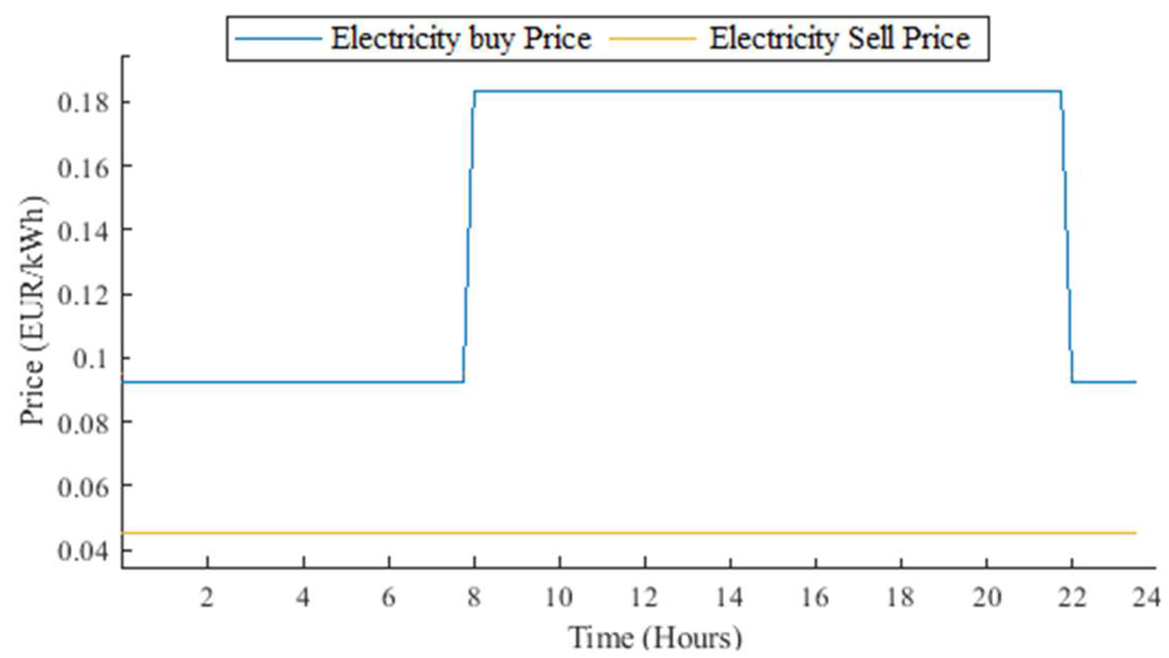
MATLAB 2022b served as the platform for conducting the simulation. The challenge of optimizing mixed integer linear programming was addressed using the TOMLAB toolbox′s CPLEX solver. A simulation was conducted on a system with a core i5 processor (11th generation) and a 64-bit operating system with 64 GB of installed RAM. The investigation revolved around the system cost implications in two scenarios aimed at cost reduction and a comparison of cost savings between the two scenarios. The findings stemmed from the 2021 Portuguese feed-in rate (0.045 EUR/kWh). In Case 1, engagement in the P2P transaction was prohibited for all participants, whereas Case 2 permitted their involvement in P2P energy sharing. In both instances, Case 1 did not yield an incentive, while Case 2 offered a rewarding outcome. The absence of LEM resulted in a system cost of EUR 103.42, whereas this cost diminished to EUR 90.10 when P2P was employed, as depicted in

Table 4. System cost.

	System Cost (EUR)
Without P2P	103.42
With P2P	90.10
Cost Saving (D) = 13.32

. Consequently, a cost reduction of EUR 13.32, or 12.9%, was obtained within this system.

In the context of Case 1, the cumulative earnings garnered by prosumers amounted to EUR 3.19. Notably, the spectrum of revenue for individual prosumers spanned from EUR 0 to 0.55, with the lowest and highest revenue figures. Conversely, in Case 2, involving P2P power exchange, the collective income produced by prosumers reached EUR 19.23, with revenue spanning from EUR 0 to 1.93. It is worth highlighting two key observations here. Initially, certain prosumers experienced minimal to almost negligible revenue due to their low power export to the grid/P2P, aligned with the aim of minimizing system costs or opting to predominantly self-consume generated power. Secondly, the revenue achieved in Case 2 significantly surpassed that of Case 1. This discrepancy stems from the P2P power transaction model, permitting prosumers to sell their excess power at a higher P2P price compared with the retail feed-in price offered by the utility grid. Simultaneously, prosumers could purchase power at a lower P2P price compared with the retail purchase price from the retailer. This pivotal difference accounts for the lower system cost in Case 2 as opposed to Case 1.

The diagram in Figure 2 illustrates the peak power export of prosumers in both scenarios. It is noticeable that the peak power export of prosumers was greater when peer-to-peer (P2P) dynamics were present. Furthermore, a subset of prosumers displayed minimal peak power export values, a reflection of the optimization model′s allowance for prosumers to self-consume generated power, thereby reducing system costs. In the absence of P2P, the range of peak power export spans from 0.005 to 4.78 kW, whereas in the presence of P2P, this range extends from 0.67 to 5.17 kW during a single time period. To allocate this cost reduction as a financial benefit to prosumers, we introduce four approaches. The concept of a circular economy serves as an incentive for existing prosumers to engage in P2P energy exchange, thereby enhancing their motivation to participate in local energy trading. Across all strategies, a shared limitation is enforced: the total monetary reward must not surpass the cost savings. In the first strategy, the cost savings are evenly divided among all prosumers. By contrast, the second strategy entails prosumers receiving 40% of the income they have produced from electricity sales to the grid or through P2P locally, as outlined in Case 2.

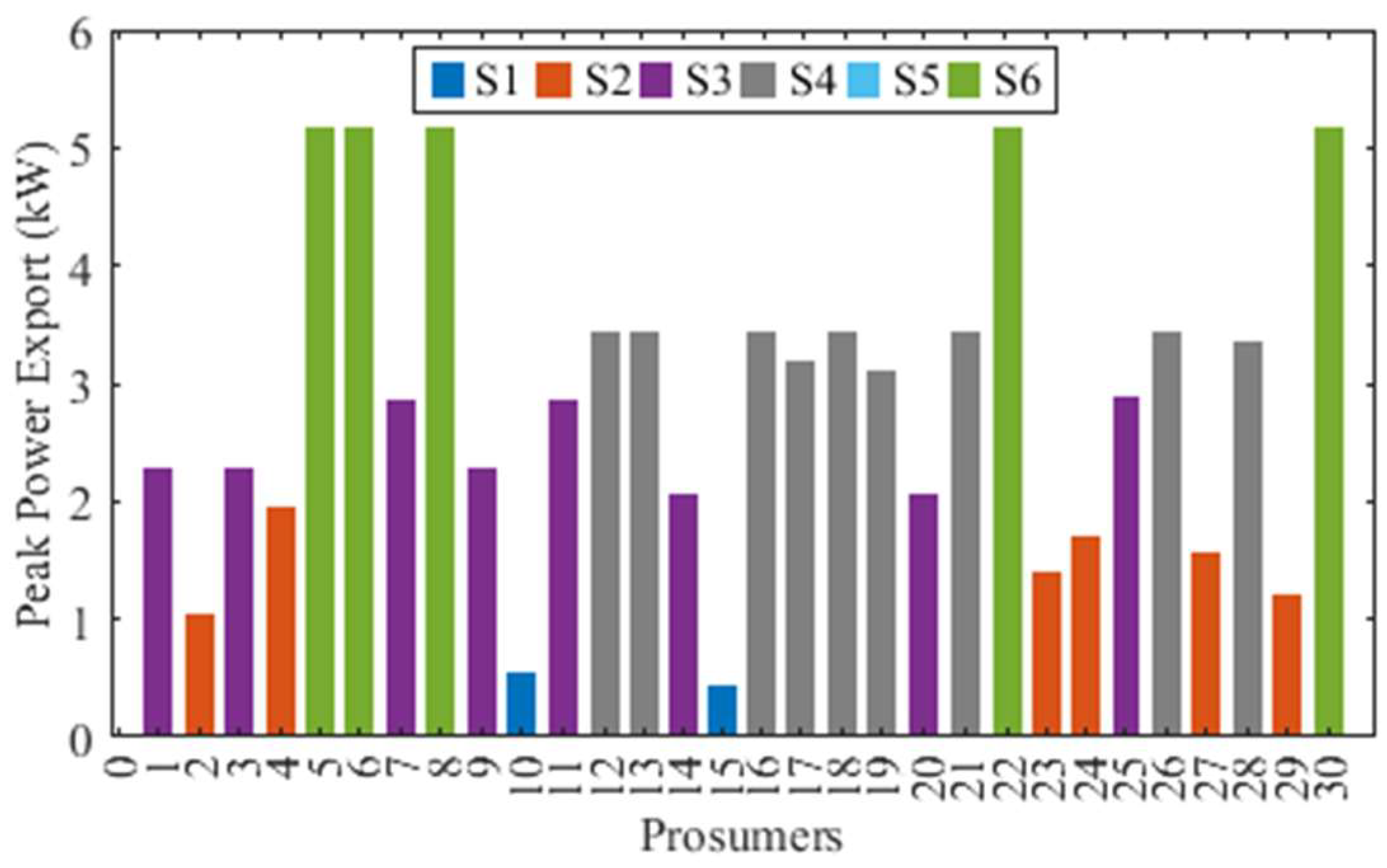
Moreover, prosumers undergo segmentation depending on their highest and average power export. Upon scrutinizing Figure 4 for Strategy 3, it becomes evident that two prosumers existed within the S1 segment, six prosumers were categorized under the S2 segment, eight prosumers were allocated to the S3 segment, nine prosumers fell into the S4 segment, no prosumers fell under the S5 segment, and five prosumers were situated within the S6 segment. All prosumers belonging to the S6 segment successfully reached the predefined maximum power export threshold of 5.175 kW. Similarly, for Strategy 4, the information presented in Figure 5 indicates the presence of six prosumers within the S1 segment, five prosumers situated in the S2 segment, two prosumers falling into the S3 segment, no prosumers in the S4 segment, three prosumers in the S5 segments, and fourteen prosumers forming the S6 segment.

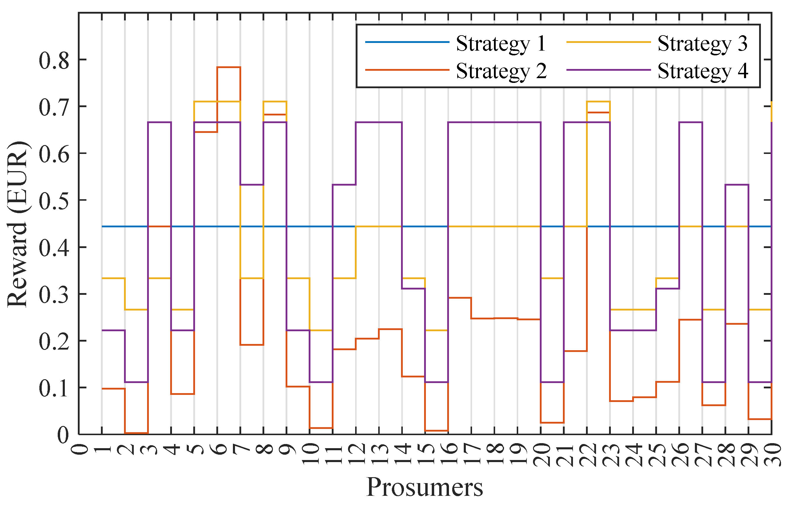
The reward amounts obtained by all prosumers across the four strategies are depicted in Figure 6. This figure enables a comparison of the rewards received by individual prosumers within each strategy. Notably, varying reward amounts were allocated to each prosumer across all four strategies. In this context, it was observed that all prosumers, categorized on the basis of their segments, attained the maximum achievable monetary rewards corresponding to their respective segments. Furthermore, a noticeable trend emerged wherein numerous prosumers within the same segment received identical rewards, a measure aimed at ensuring that the aggregate rewards distributed among all prosumers remained beneath the threshold of cost savings. We also experimented with introducing a constraint to prevent prosumers within the same segment from receiving identical rewards. This led to varying reward amounts for prosumers within the same segment, but the collective sum of rewards remained significantly lower than the achieved cost savings. Given that the primary objective of the study was to optimize rewards and make the most efficient use of cost savings, outcomes with diverse reward amounts were disregarded as suboptimal. The ultimate results based on the proposed segmentation criteria and reward limitations reflected the highest level of cost savings utilization and reward maximization. Additionally,

Table 5. Incentive statistics.

Strategy	Min Reward (EUR)	Max Reward (EUR)	Average Reward (EUR)	Overall Incentive (EUR)
Strategy 1	0.444 (Identical to all)			13.32
Strategy 2	0.003	0.784	0.241	7.24
Strategy 3	0.222	0.710	0.408	12.25
Strategy 4	0.110	0.667	0.444	13.32

presents a comparison of the least, extreme, average, and full incentive values.

Comparing the results with three-segment strategies, as shown in Figure 7, the total reward in Strategy 3 increases up to 1.63% from EUR 12.05 to 12.25, while in Strategy 4, a remarkable increment by 13.73% from EUR 11.49 to 13.32 is obtained.

7. Conclusions

This empirical study focused on a setup involving 30 prosumers utilizing photovoltaic systems and storage alongside 6 consumers. The resolution of the mixed integer linear programming problem was achieved in MATLAB using the CPLEX solver from the TOMLAB toolbox. The results indicate that across all proposed methods, the total reward remains either lesser or equal to the cost savings. Implementing these recommended strategies can lead to the maximization of customer profits. LEM system operators can utilize these strategies to enhance the interest of energy consumers in participating in P2P arrangements. This innovative approach has the potential to help both consumers and power distributors overcome substantial challenges within the P2P framework. The inclusion of more prosumers in P2P has the potential to reduce dependence on grid power imports. The six-segment strategy ensures the maximization of the financial earnings of prosumers. Both Strategy 3 and Strategy 4 provided better results in the six segments of prosumers compared with the three segments. Specifically, Strategy 4 exploits the entire cost savings of 12.9% as a reward for prosumers.

In this study, it was presumed that the necessary setup for power flow and communication were available. The practical implementation of the proposed model would require all the above-mentioned facilities to be available. Further investigations could explore areas such as multi-aggregator systems, new segmentation criteria, innovative incentive approaches, and incorporating cost-saving measures into the limits.

References

1. Tushar, W.; Nizami, S.; Azim, M.; Yuen, C.; Smith, D.; Saha, T.; Poor, H. Peer-to-Peer Energy Sharing: A Comprehensive Review. Found. Trends Electr. Energy Syst. 2023, 6, 1–82. [Google Scholar] [CrossRef]
2. Iria, J.; Soares, F. Real-time provision of multiple electricity market products by an aggregator of prosumers. Appl. Energy 2019, 255, 113792. [Google Scholar] [CrossRef]
3. Dynge, M.F.; Berg, K.; Bjarghov, S.; Cali, U. Local electricity market pricing mechanisms’ impact on welfare distribution, privacy and transparency. Appl. Energy 2023, 341, 121112. [Google Scholar] [CrossRef]
4. Duvignau, R.; Heinisch, V.; Göransson, L.; Gulisano, V.; Papatriantafilou, M. Benefits of small-size communities for continuous cost-optimization in peer-to-peer energy sharing. Appl. Energy 2021, 301, 117402. [Google Scholar] [CrossRef]
5. Hampton, H.; Foley, A.; Del Rio, D.; Sovacool, B. Developing future retail electricity markets with a customer-centric focus. Energy Policy 2022, 168, 113147. [Google Scholar] [CrossRef]
6. De Martini, P.; Gallagher, L.; Takayesu, E.; Hanley, R.; Henneaux, P. Unlocking Consumer DER Potential: Consumer-Centric Approaches for Grid Services. IEEE Power Energy Mag. 2022, 20, 76–84. [Google Scholar] [CrossRef]
7. Lu, X.; Guo, H. Trust-DETM: Distributed Energy Trading Model Based on Trusted Execution Environment. Mathematics 2023, 11, 2934. [Google Scholar] [CrossRef]
8. Jalalzad, S.H.; Salehizadeh, M.R.; Haghighi, R. Integration of Community Energy Storage for Congestion Management and Energy Cost Optimization: A TLBO Solution Approach. Res. Technol. Electr. Ind. 2022, 1, 211–220. [Google Scholar] [CrossRef]
9. Haghighi, R.; Jalalzad, S.; Salehizadeh, M.; Alhelou, H.; Siano, P. Cloud Energy Storage Investment by Collaboration of Microgrids for Profit and Reliability Enhancement Considering a TSO-DSO Yearly Reward. IEEE Access 2023, 11, 23808–23826. [Google Scholar] [CrossRef]
10. Nezamabadi, H.; Vahidinasab, V. Arbitrage Strategy of Renewable-Based Microgrids via Peer-to-Peer Energy-Trading. IEEE Trans. Sustain. Energy 2021, 12, 1372–1382. [Google Scholar] [CrossRef]
11. Neagu, B.-C.; Ivanov, O.; Grigoras, G.; Gavrilas, M. A New Vision on the Prosumers Energy Surplus Trading Considering Smart Peer-to-Peer Contracts. Mathematics 2020, 8, 235. [Google Scholar] [CrossRef]
12. Kuno, S.; Tanaka, K.; Yamada, Y. Effectiveness and Feasibility of Market Makers for P2P Electricity Trading. Energies 2022, 15, 4218. [Google Scholar] [CrossRef]
13. Koengkan, M.; Fuinhas, J.; Osmani, F.; Kazemzadeh, E.; Auza, A.; Alavijeh, N.; Teixeira, M. Do financial and fiscal incentive policies increase the energy efficiency ratings in residential properties? A piece of empirical evidence from Portugal. Energy 2022, 241, 122895. [Google Scholar] [CrossRef]
14. Trivedi, R.; Patra, S.; Sidqi, Y.; Bowler, B.; Zimmermann, F.; Deconinck, G.; Papaemmanouil, A.; Khadem, S. Community-Based Microgrids: Literature Review and Pathways to Decarbonise the Local Electricity Network. Energies 2022, 15, 918. [Google Scholar] [CrossRef]
15. Kim, S.; Yoon, Y.; Jin, Y. Price-Guided Peer-To-Peer Trading Scheme and Its Effects on Transaction Costs and Network Losses. Energies 2022, 15, 8274. [Google Scholar] [CrossRef]
16. Mochi, P.; Pandya, K.; Faia, R.; Soares, J. Prosumer Segmentation Strategies for Local Electricity Market Partaking by Monetary Reward. IEEE Access 2023, 11, 62879–62891. [Google Scholar] [CrossRef]
17. Coursera Course on Customer Value in Pricing Strategy. Available online: https://www.coursera.org/learn/uva-darden-bcg-pricing-strategy-customer-value (accessed on 29 April 2023).
18. Mochi, P.; Pandya, K. The Impact of Social Nudge on System Cost & Revenue Optimization in Local Electricity Market. In Proceedings of the 2023 International Conference on Power Electronics and Energy (ICPEE), Bhubaneswar, India, 3–5 January 2023; pp. 1–5. [Google Scholar] [CrossRef]
19. Mochi, P.; Pandya, K. Two Stage Optimization for Customer Fiscal Incentive in Local Electricity Market. In Proceedings of the 2022 IEEE International Power and Renewable Energy Conference (IPRECON), Kollam, India, 16–18 December 2022; pp. 1–6. [Google Scholar] [CrossRef]
20. Mochi, P.; Pandya, K.; Soares, J.; Vale, Z. Optimizing Power Exchange Cost Considering Behavioral Intervention in Local Energy Community. Mathematics 2023, 11, 2367. [Google Scholar] [CrossRef]
Figure 1. Block diagram of proposed methodology.
Mathematics 11 03933 g001
Figure 2. Battery and PV power capacity.
Mathematics 11 03933 g002
Figure 3. Price for power buy/sell.
Mathematics 11 03933 g003
Figure 4. Prosumer segments in Strategy 3.
Mathematics 11 03933 g004
Figure 5. Prosumer segments in Strategy 4.
Mathematics 11 03933 g005
Figure 6. Prosumer reward comparison.
Mathematics 11 03933 g006
Figure 7. Comparison of three-segment and six-segment reward.
Mathematics 11 03933 g007