On the Stability of a Convective Flow with Nonlinear Heat Sources

Abstract

The linear stability of a convective flow in a vertical fluid layer caused by nonlinear heat sources in the presence of cross-flow through the walls of the channel is investigated in this paper. This study is relevant to the analysis of factors that affect the effectiveness of biomass thermal conversion. The nonlinear problem for the base flow temperature is investigated in detail using the Krasnosel’skiĭ–Guo cone expansion/contraction theorem. It is shown that a different number of solutions can exist depending on the values of the parameters. Estimates for the norm of the solutions are obtained. The linear stability problem is solved numerically by a collocation method based on Chebyshev polynomials. It is shown that the increase in the cross-flow intensity stabilizes the flow, but there is also a small region of the radial Reynolds numbers where the flow is destabilized.

1. Introduction

The development of renewable energy sources is crucial for the sustainability of our society. Biomass thermal conversion is considered to be one of the promising alternatives for heat generation. Thermal conversion is a process where biomass is burned in a chamber producing heat. Different methods of biomass thermal conversion are discussed in a recent survey [1]. Experimental studies [2,3] indicate that several factors may affect the efficiency of the conversion process—the co-firing of propane or microwave pre-treatment of biomass.

Combustion can also occur in porous media. A recent survey [4] discusses challenges and developments in porous media combustion technology. Biomass conversion using porous materials is analyzed in the review paper [5]. Another widely used application of flows through porous walls of a channel is dynamic filtration—one of the most popular methods for purifying fluids. In this method, a fluid with contaminants passes through a porous wall so that the pure fluid flows out of the wall while contaminants are left in the channel [6,7,8].

The analysis of processes that occur during biomass thermal conversion represents a complex multiphysics problem where different factors that affect the conversion process should be taken into account (convection, chemical reactions, external electric and magnetic field, to mention just a few). The following three approaches are often used to analyze complex phenomena in science and engineering: (a) experimental studies, (b) numerical modeling and (c) stability analysis. In the present paper mwe use stability analysis in an attempt to understand the role of each factor (included in the model) in the stability of a base flow caused by internal heat generation. Heat is released in the fluid as a result of a chemical reaction. In addition, the walls of the channel where the flow takes place are assumed to be permeable. An investigation of the stability of a fluid flow can be used to address the following issues: (1) finding the values of the parameters of the problem for which the flow is linearly stable, and (2) determining the factors that either delay or enhance instability. In some applications, instability is undesirable (for example, a high degree of turbulence in air may cause problems for airplane safety). There are also applications where instability is desirable. As is shown in [9], the intense heat transfer and mixing provide good conditions for combustion that, in turn, lead to more efficient energy conversion. Thus, instability should be stimulated to achieve more favorable conditions for biomass thermal conversion. Methods of hydrodynamic stability for both isothermal and non-isothermal flows are considered in several monographs (see, for example, [10,11]).

Flows with internal heat generation represent considerable interest due to numerous applications: neutron irradiation in thermonuclear reactors [12], convection in the Earth’s mantle [13], and biomass thermal conversion [1]. The linear stability of a convective flow in a vertical fluid layer caused by uniform heat generation is investigated in several papers (see [14,15,16]). The effect of the Prandl number of the instability boundary is explored in [14] and later in [17], where it is shown that the increase in the Prandtl number leads to the appearance of a buoyant mode. This mode is associated with a rapid decrease in the critical Grashof number. In addition, the most unstable perturbation is represented by a thermal running wave that propagates downstream with a sufficiently large phase velocity. Linear stability analysis of a convective flow due to heat sources of constant density in a tall vertical annulus is conducted in [18]. Calculations show that axisymmetric perturbations are the most unstable for relatively small gaps while the spiral mode is the most unstable one for wide gaps. A similar analysis is also conducted in [19], where the results of linear stability calculations for a convective flow in a pipe are compared with experimental data. Both the theory and experiment predict the same form of the most unstable mode (spiral perturbation). The stability of a combined base flow caused by uniform heat generation, external pressure gradient and different temperatures of the walls is investigated in [20]. Marginal stability curves become more complicated with multiple minima.

The effect of nonlinear heat sources on the stability boundary for a convective flow in a vertical fluid layer is analyzed in [21], where the existence of several solutions of the nonlinear boundary value problem for the base flow temperature is shown numerically. The linear stability of a flow due to nonlinear heat sources in a tall vertical annulus is investigated in [22] for both asymmetric and axisymmetric perturbations. It is shown in [22] that, for wide gaps, asymmetric (spiral) perturbations are the most unstable ones. The combined effect of nonlinear heat sources and different wall temperatures on the linear stability characteristics is analyzed in [23]. Calculations show that two modes of instability can be present, shear or buoyant instability, depending on the value of the Prandtl number.

The mathematical model used in the paper consists of a coupled system of Navier–Stokes equations and a heat equation where the density of internal heat sources is a nonlinear function of temperature (heat is released as a result of a chemical reaction that takes place in a combustion chamber). Thus, even the equations for the base flow become nonlinear (in contrast with classical problems in hydrodynamic stability theory, where a base flow is usually obtained analytically from the equations of motion). As a result, questions on the existence and uniqueness of the solution of the corresponding nonlinear boundary value problem for a system of ordinary differential equations (describing the base flow) should be answered. This is important for the case where a nonlinear problem has several solutions so that the “correct solution” should be selected for linear stability analysis.

The main contributions of the present study are summarized as follows.

• The analysis of the nonlinear boundary value problem for the temperature distribution is performed using rigorous mathematical tools such as Krasnosel’skiĭ–Guo cone expansion/contraction theorem. It is shown in the paper that, depending on the value of the Frank–Kamenetskii parameter (characterizing the thermal effect of the reaction), the number of solutions is 0, 1 or 2.
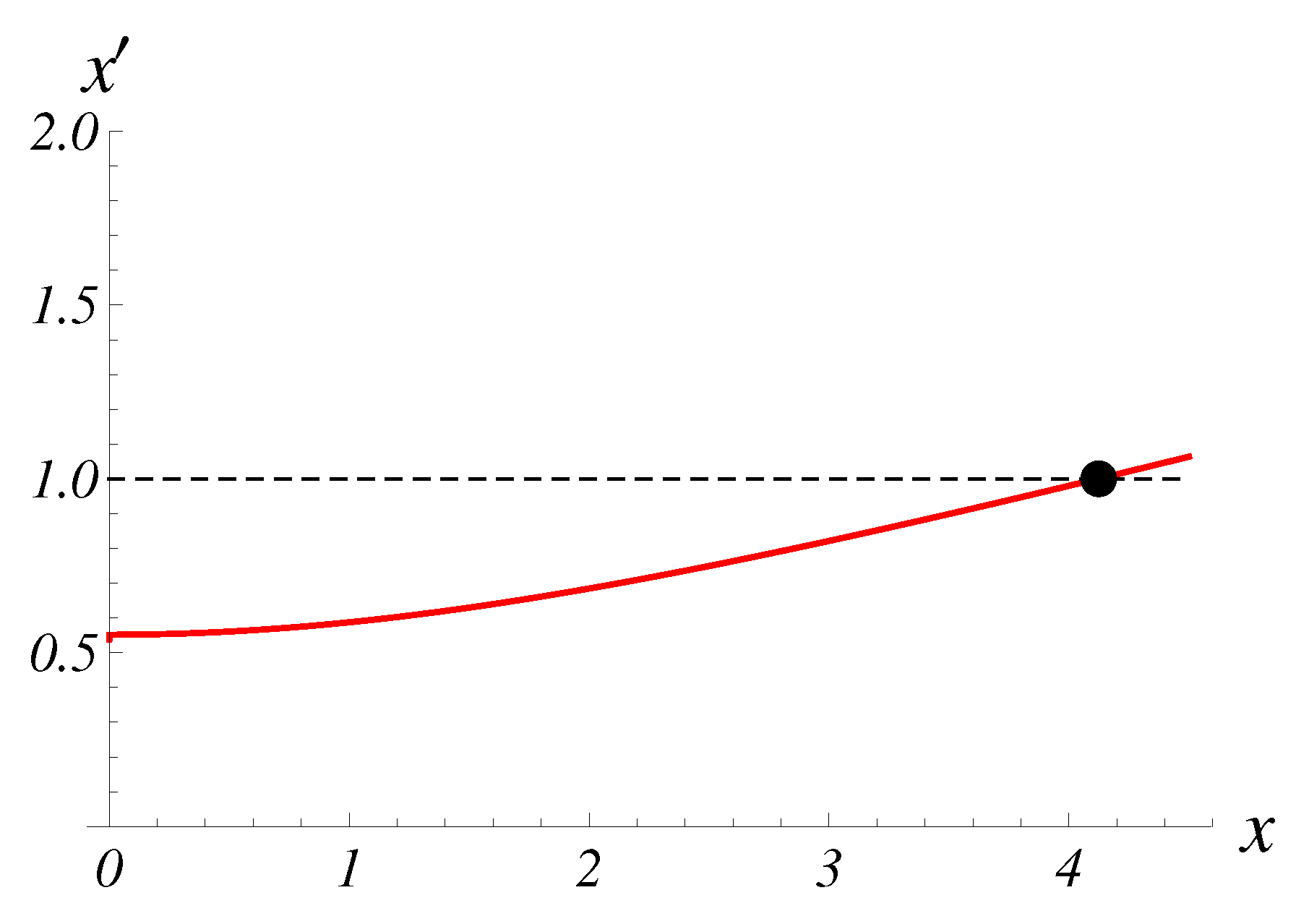
• In addition, it is proved that in the region of interest for linear stability analysis, there are two solutions of the nonlinear boundary value problem such that the maximum norm of one solution is smaller than 1 while the maximum norm of the second solution is larger than 1. This gives a simple criterion for the base flow selection—a physically realizable solution is with the smallest maximum norm—and this solution should be chosen for stability analysis.
• Bifurcation analysis is performed to numerically investigate the effect of the parameters of the problem on bifurcation diagrams.
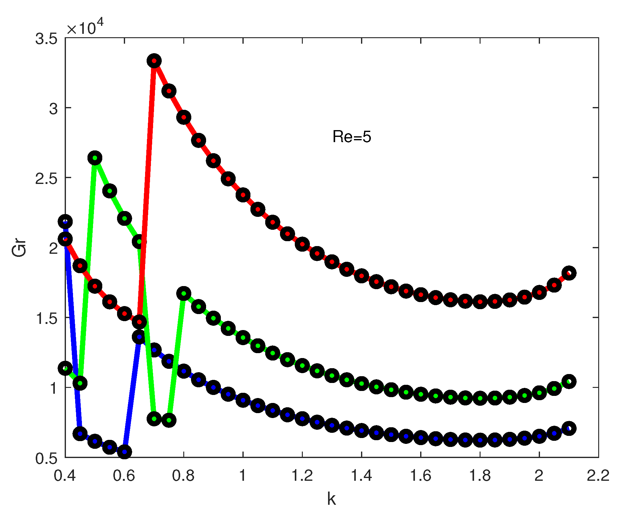
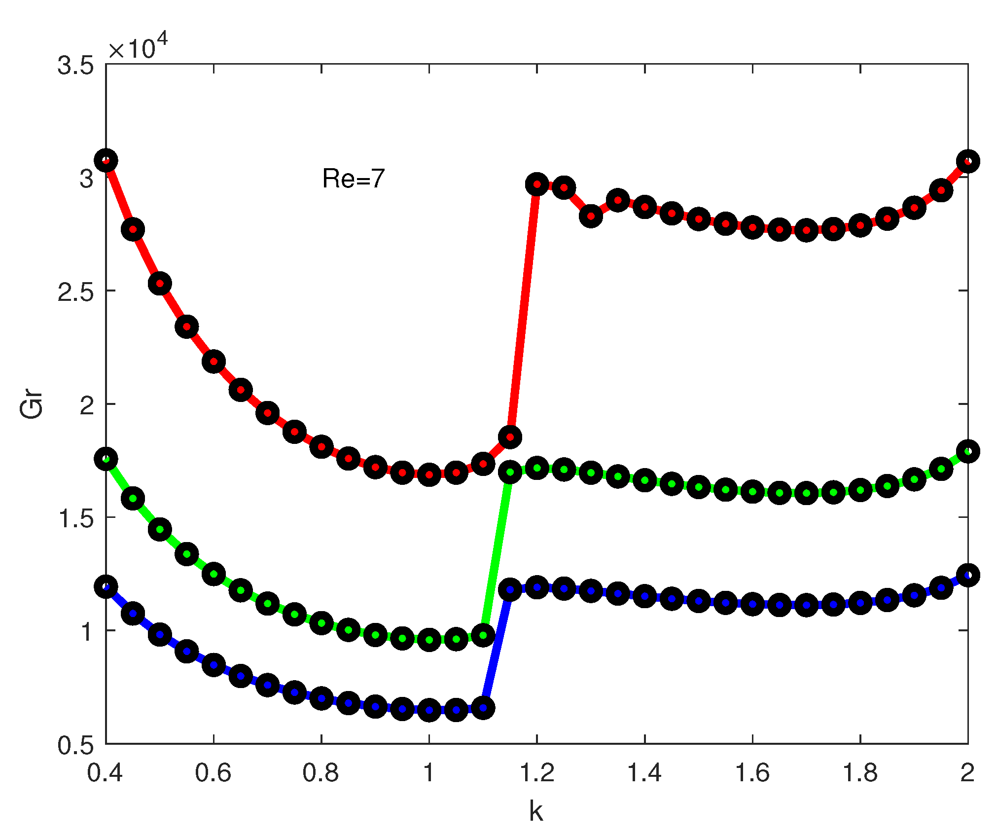
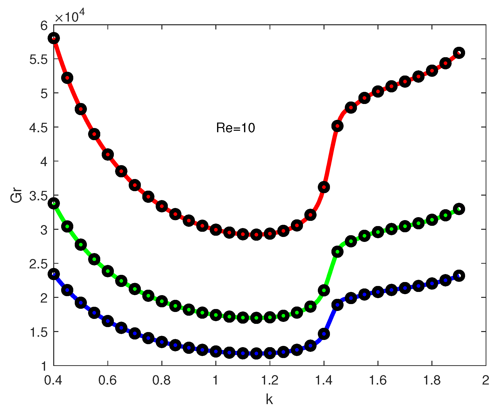
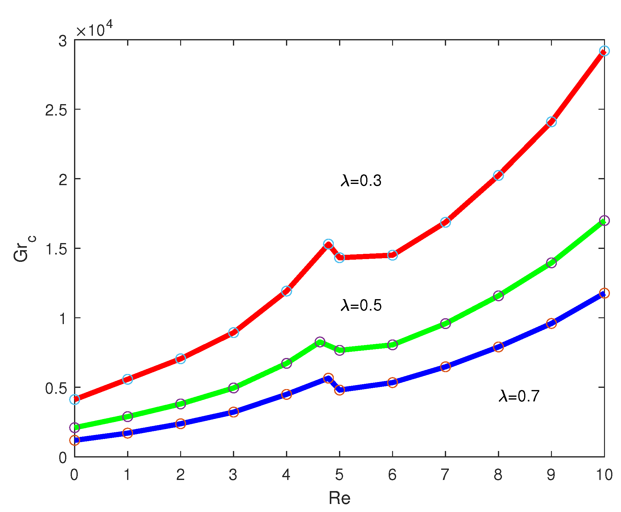
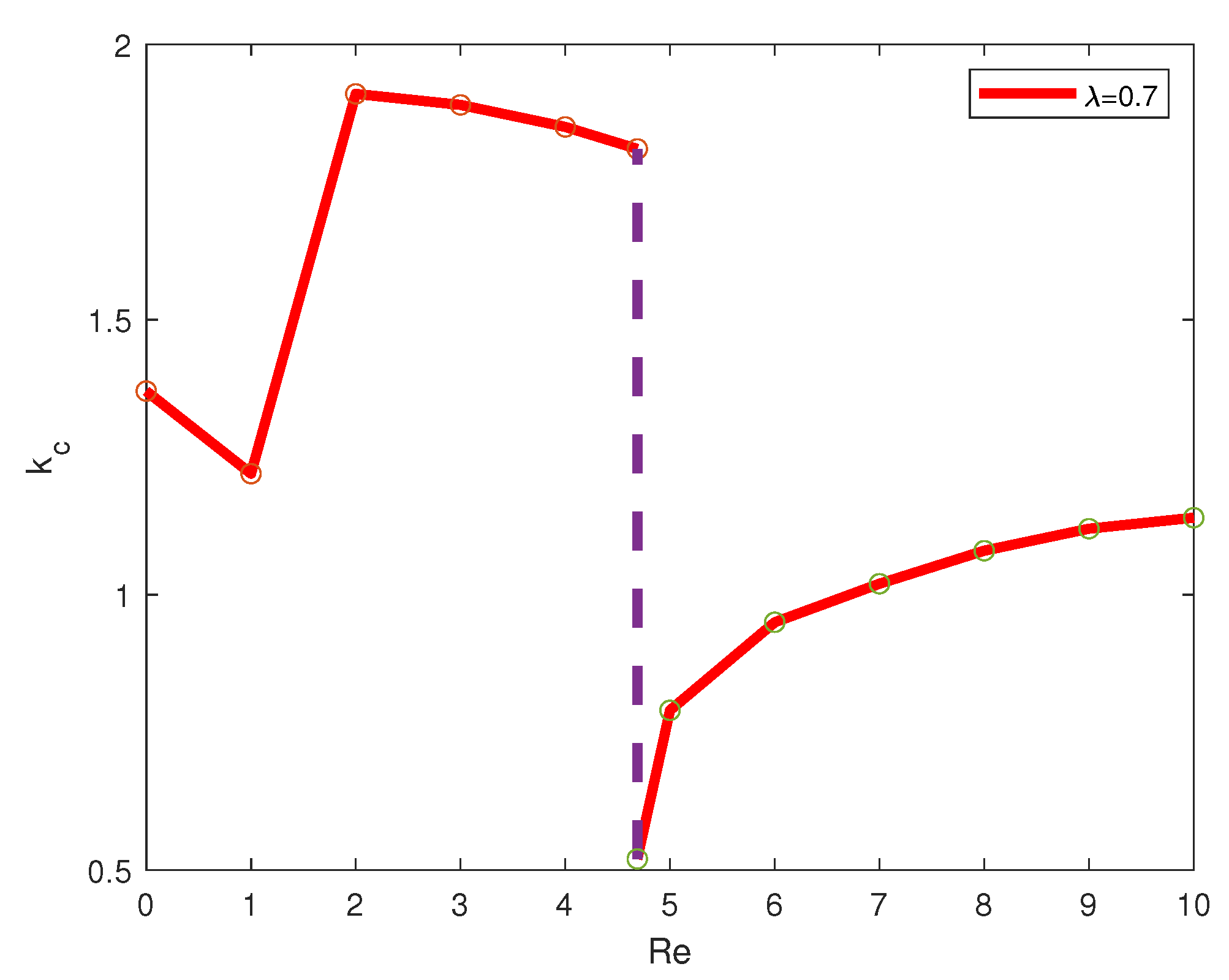
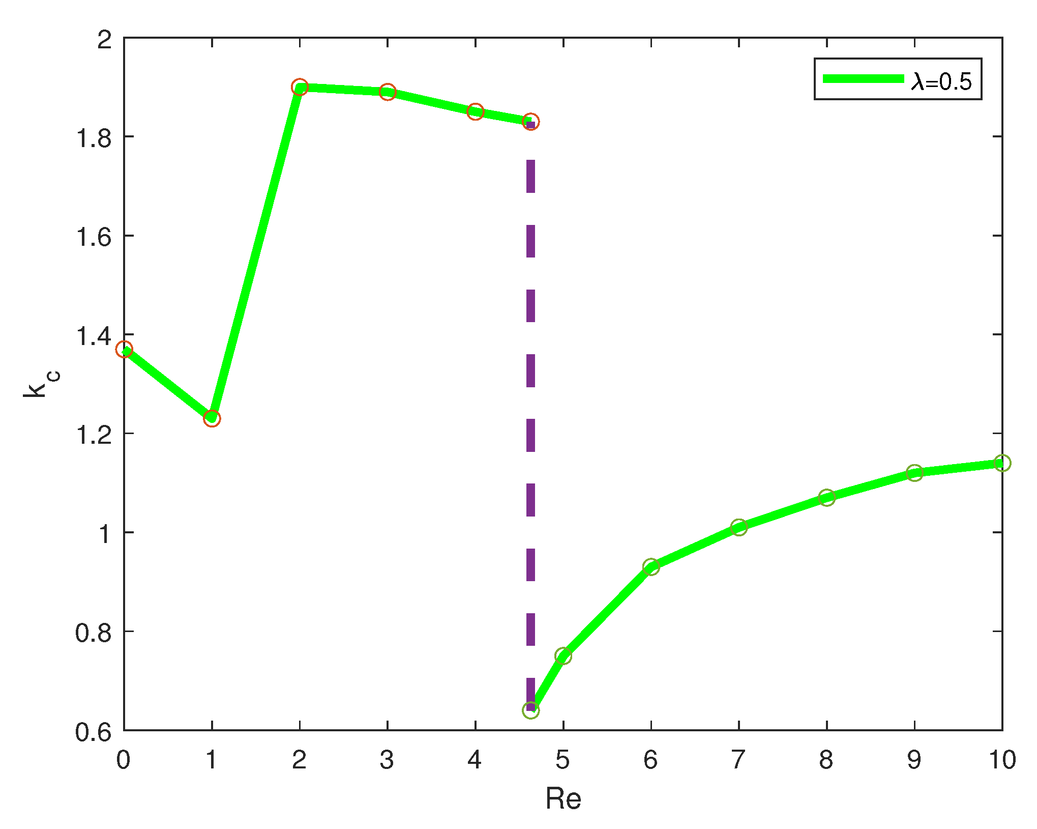
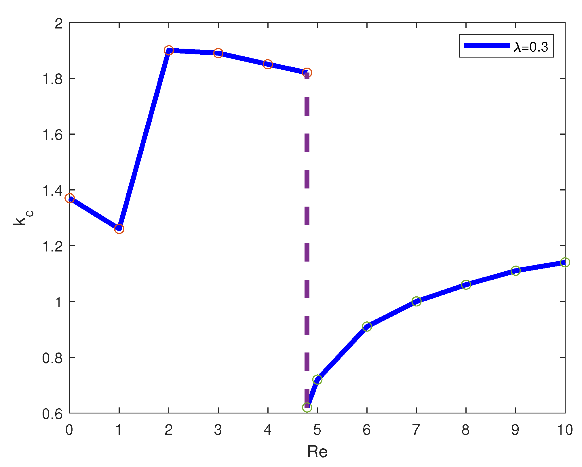
• A linear stability problem is formulated and solved numerically for different values of the parameters characterizing the problem: the Frank–Kamenetskii parameter $\lambda$ and the Reynolds number $Re$ (based on the velocity of the flow through permeable walls). Critical values of the Grasshof number are found for different values of $\lambda$ and $Re$.
• Recommendations for the choice of parameters that result in more intensive mixing are provided.

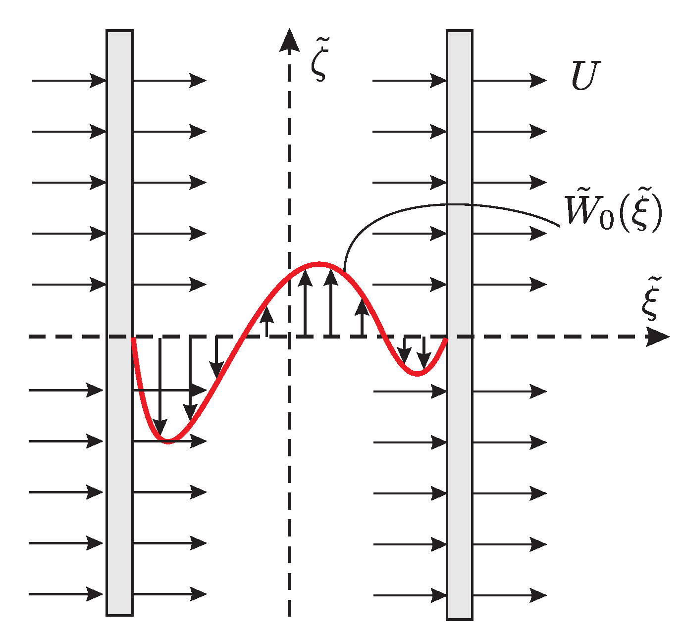
2. Mathematical Formulation of the Problem

Consider a flow of a viscous chemically reacting incompressible fluid in a vertical channel formed by two infinite parallel planes $\tilde{\xi }=\pm h$ (see Figure 1). A Cartesian coordinate system $(\tilde{\xi },\tilde{\eta },\tilde{\zeta })$ with the origin at the axis of the channel is selected, and the $\tilde{\zeta }$-axis is directed upwards. The following convention is used throughout the paper: all variables with tildes are dimensional while the variables without tildes are dimensionless. The walls are kept at equal constant temperature ${\theta }_0$. It is assumed that there is a flow with constant velocity $\pm U\mathbf{i}$ through permeable walls of the channel in the direction perpendicular to the planes, where $\mathbf{i}$ is the unit vector in the $\tilde{\xi }$-direction. Positive and negative signs correspond to flows in the positive or negative $\tilde{\xi }$-directions, respectively. The base flow velocity distribution ${\tilde{W}}_0(\tilde{\xi }$) due to internal heat sources is also shown in Figure 1.

It is assumed that the thermal effect of the reaction is large enough so that one can neglect the dependence of the heat generation on the concentration of the reagent. In this case, convective flow in the vertical direction is generated by internal heat generation, where the density of the internal heat sources Q is described by Arrhenius’ law:

$$Q=Q_0{e}^{-E/\left(R\tilde{T}\right)},$$

(1)

where $Q_0$ is the parameter characterizing the thermal effect of the reaction, E is the activation energy, R is the universal gas constant and $\tilde{T}$ is the absolute temperature. The use of Arrhenius’ Equation (1) for the analysis of pyrolysis conversion (the procedure that converts biomass into liquid fuels called bio-oils) is considered in [24,25]. The movement of the fluid in the channel is described by the dimensionless system of the Navier–Stokes equations under the Boussinesq approximation:

$$\begin{array}{ccc}\hfill \frac{\partial \mathbf{v}}{\partial \tau }+Gr(\mathbf{v}·\nabla )\mathbf{v}& =& -\nabla p+\Delta \mathbf{v}+\mathrm{\Theta }\mathbf{k},\hfill \end{array}$$

(2)

$$\begin{array}{ccc}\hfill \frac{\partial \mathrm{\Theta }}{\partial \tau }+Gr\mathbf{v}·\nabla \mathrm{\Theta }& =& \frac{\Delta \mathrm{\Theta }}{Pr}+\lambda \frac{e^{\mathrm{\Theta }}}{Pr},\hfill \end{array}$$

(3)

$$\begin{array}{ccc}\hfill \nabla ·\mathbf{v}& =& 0.\hfill \end{array}$$

(4)

Here, $\mathbf{v}$, $\mathrm{\Theta }$ and p are the dimensionless velocity vector, temperature and pressure, $\tau$ is time and $\mathbf{k}=(0,0,1)$. The Boussinesq approximation is considered in detail in many papers and books (see, for example, [26,27,28,29,30]). The main assumptions of the Boussinesq approximation can be formulated as follows: (a) the non-uniformity of fluid density caused by changes in pressure is small and is neglected, and (b) the non-uniformity of density caused by non-uniform temperature distribution is assumed to be small so that the density is given by

$$\tilde{\rho }=\rho (1-\beta \tilde{T}),$$

(5)

where $\rho$ is a constant and $\beta$ is the coefficient of the thermal expansion. Moreover, the change in density with respect to the temperature is taken into account only in the buoyancy term (the last term in (2)) while, in the other terms in (2) and (3), the density is assumed to be constant. Note that there are situations where the Boussinesq approximation may lead to incorrect results (for example, in astrophysical MHD simulations). The limitations of the use of the Boussinesq approximation have recently been described in detail (see [31,32,33]). The detailed derivation of the dimensionless form of Equations (2)–(4) and the analysis of the Boussinesq approximation are found elsewhere (see, for example, [29]), and are not shown here for brevity. Note that we have used the Frank–Kamenetskii transformation [34]. The idea is very simple—expand the exponent in (1) in a Taylor series and keep only the linear term of the expansion. The accuracy of the transformation is analyzed in [34,35,36], where it is shown that the error in using it for a typical set of parameters is about 5%. The main advantage of using the transformation is related to the fact that the last term on the right-hand side of (3) is much easier to work with mathematically than the exponent in (1). System (2)–(4) is made dimensionless by choosing the following values as the measures of length, h, time, $h^2/\nu$, temperature, $R{\theta }_0^2/E$, velocity, $g\beta h^{2}R{\theta }_0^2/\left(\nu E\right)$ and pressure, $\rho g\beta hR{\theta }_0^2/E$, respectively. Here, $\nu$ is the kinematic viscosity of the fluid, and g is the acceleration due to gravity. The problem contains four dimensionless parameters: the Grashof number $Gr=g\beta R{\theta }_0^2{h}^3/\left({\nu }^{2}E\right)$, the Prandtl number $Pr=\nu /\chi$, the Frank–Kamenetskii parameter $\lambda =Q_{0}E{h}^2/\left(\kappa R{\theta }_0^2\right)exp(-E/\left(R{\theta }_0\right))$ and the Reynolds number $Re=Uh/\nu$. Here, $\chi$ and $\kappa$ are the thermal diffusivity and thermal conductivity of the fluid, respectively.

There exists a steady flow of the following form:

$${\mathbf{v}}_{\mathbf{0}}=(U,0,W_0\left(\xi \right)),\mathrm{\Theta }={\mathrm{\Theta }}_0\left(\xi \right),p=p_0\left(\zeta \right).$$

(6)

Substituting (6) into (2)–(4), we obtain the system of ordinary differential equations describing the base flow:

$$\begin{array}{ccc}\hfill -\frac{d{p}_0}{d\zeta }+W_0^{{}^{″}}-Re{W}_0^{{}^{\prime }}+{\mathrm{\Theta }}_0& =& 0,\hfill \end{array}$$

(7)

$$\begin{array}{ccc}\hfill {\mathrm{\Theta }}_0^{{}^{″}}-RePr{\mathrm{\Theta }}_0^{{}^{\prime }}+\lambda e^{{\mathrm{\Theta }}_0}& =& 0.\hfill \end{array}$$

(8)

The boundary conditions are

$$W_0(\pm 1)=0,{\mathrm{\Theta }}_0(\pm 1)=0.$$

(9)

It is assumed that the channel is closed by top and bottom lids (located at $\pm \infty$) so that the following condition is satisfied:

$${\int }_{-1}^1{W}_0\left(\xi \right)d\xi =0.$$

(10)

In practice, the base flow considered in the paper takes place in the middle portion of a sufficiently high vertical channel with a large aspect ratio. One can observe that (a) nonlinearity appears only in Equation (8) and (b) the boundary value problem for ${\mathrm{\Theta }}_0$ can be solved separately. If ${\mathrm{\Theta }}_0$ would be known, then one can determine $W_0$ from (7) and (9). In addition, constant $d{p}_0/d\zeta$ is determined from (10). In a classical hydrodynamic stability theory, the base flow is usually determined as an exact solution of the equations of motion. Different approaches are used in the literature to construct exact solutions (see, for example, Refs. [37,38] for the case of isothermal flows and [39] for convective flows). Since a closed form solution to (8) and (9) is not available, problem (7)–(10) has to be solved numerically. Thus, the properties of the boundary value problem (7)–(10) such as the existence and multiplicity of solutions are determined by the boundary value problem for the function ${\mathrm{\Theta }}_0$. Different mathematical tools are used in the literature to prove the existence of solutions (see, for example, Ref. [40] for incompressible Navier–Stokes equations). Rigorous mathematical analysis of these properties is the subject of investigation in the next subsection.

3. Nonlinear Boundary Value Problem

We rewrite Equation (8) and the boundary conditions for ${\mathrm{\Theta }}_0$ in the form

$$x^{″}+\alpha x^{\prime }+\lambda e^x=0,x(-1)=0,x\left(1\right)=0.$$

(11)

Here, $\lambda$ is a positive number and $\alpha =-RePr$ is a real number. We are interested in positive solutions of the two parameter boundary value problem (11). A solution x of (11) is said to be positive if $x\left(t\right)>0$ for every $t\in (-1,1)$. The next proposition can be easily proved.

Proposition 1. 

The following statements are valid.

1. 

The zero function $x\equiv 0$ is not a solution of (11).

2. 

A function x solves (11) if and only if $y\left(t\right):=x(-t)$ solves

$$y^{″}+(-\alpha )y^{\prime }+\lambda e^y=0,y(-1)=0,y\left(1\right)=0;$$

(12)

besides, $y^{\prime }(-1)=-x^{\prime }\left(1\right)$ and $y^{\prime }\left(1\right)=-x^{\prime }(-1)$.

3. 

If x is a positive solution of (11), then $x^{\prime }(-1)>0$ and $x^{\prime }\left(1\right)<0$.

4. Some Preliminaries

In this section, we will assume that $\alpha$ is positive.

4.1. Linear Part of the Problem

Let $Q:=\left\{(t,s)\in {\mathbb{R}}^2:\left|t\right|\le 1,\left|s\right|\le 1\right\}$. Denote by $\stackrel{\circ }{Q}$ and $\partial Q$ the interior and the boundary of Q, respectively.

The linear homogeneous problem

$$x^{″}+\alpha x^{\prime }=0,x(-1)=0=x\left(1\right)$$

(13)

has only the trivial solution; thus (see [41], Theorem 2.4), there exists a unique Green’s function, $g(t,s)$, related to (13). By using a Green’s function Mathematica package, see [41], we find

$$g(t,s)=\left\{\begin{array}{ccc}{\displaystyle \frac{(e^{\alpha (s+1)}-1)e^{-\alpha t}(e^{\alpha t}-e^{\alpha })}{\alpha (e^{2\alpha }-1)},}& \mathrm{if}& -1\le s\le t\le 1,\\ {\displaystyle \frac{(e^{\alpha (t+1)}-1)e^{-\alpha t}(e^{\alpha s}-e^{\alpha })}{\alpha (e^{2\alpha }-1)},}& \mathrm{if}& -1\le t<s\le 1.\end{array}\right.$$

(14)

The function g has the properties listed in ([41], Definition 2.1); in particular, g is continuous on Q. Let us introduce a function $k:Q\to Q$,

$$k(t,s):=-g(t,s),(t,s)\in Q,$$

and a function $\mathrm{\Phi }:[-1,1]\to [-1,1]$,

$$\mathrm{\Phi }\left(s\right):=k(s,s)=\frac{\left(e^{\alpha (1+s)}-1\right)\left(e^{\alpha (1-s)}-1\right)}{\alpha (e^{2\alpha }-1)},s\in [-1,1].$$

(15)

Proposition 2. 

The functions k and Φ have the following properties.

1. 

$k(t,s)>0$ for every $(t,s)\in \stackrel{\circ }{Q}$ and $k(t,s)=0$ for every $(t,s)\in \partial Q$.

2. 

$\mathrm{\Phi }\left(s\right)>0$ for every $s\in (-1,1)$ and $\mathrm{\Phi }(\pm 1)=0$.

3. 

$k(t,s)\le \mathrm{\Phi }\left(s\right)$ for every $t,s\in [-1,1]$.

4. 

Let a and b be two real numbers such that $-1<a<b<0$. Let

$$c_1:=\frac{e^{\alpha (1-b)}-1}{e^{2\alpha }-1},c_2:=\frac{e^{2\alpha }-e^{\alpha (1-a)}}{e^{2\alpha }-1},c:=min\{c_1,c_2\}.$$

(16)

Then, $c\in (0,1)$ and $c\mathrm{\Phi }\left(s\right)\le k(t,s)$ for every $t\in [a,b]$ and every $s\in [-1,1]$.

Proof. 

The assertions (1)–(4) are valid by straightforward calculations. Regarding (4), we only note that (a) $c_1\mathrm{\Phi }\left(s\right)\le k(t,s)$ for every $t\in [a,b]$ and every $s\in [-1,1]$ such that $-1\le s\le t\le 1$; (b) $c_2\mathrm{\Phi }\left(s\right)\le k(t,s)$ for every $t\in [a,b]$ and every $s\in [-1,1]$ such that $-1\le t<s\le 1$.    □

The properties (3) and (4) in Proposition 2 are inspired by [42].

4.2. Integral Operator

Taking into account ([41], Theorem 2.4), we see that x is a solution of the boundary value problem (11) if and only if x is a solution of the integral equation

$$x\left(t\right)=\lambda {\int }_{-1}^{1}k(t,s)e^{x\left(s\right)}ds,t\in [-1,1].$$

(17)

We will consider the Banach space $C_{[-1,1]}$ with the norm $\parallel x\parallel :=\underset{-1\le t\le 1}{max}\left|x\left(t\right)\right|$. Define an integral operator $T:C_{[-1,1]}\to C_{[-1,1]}$,

$$Tx\left(t\right):=\lambda {\int }_{-1}^{1}k(t,s)e^{x\left(s\right)}ds,x\in C_{[-1,1]},t\in [-1,1].$$

(18)

In view of (17), the fixed points of T coincide with the solutions of (11).

Definition 1 

([43], pp. 1–2). Let E be a Banach space. A nonempty convex closed subset M of E is called a cone if (a) $\lambda x\in M$ for every $x\in M$ and every $\lambda \ge 0$; (b) $x\in M$, $-x\in M$ implies $x=\theta$, where θ is the zero element of E.

Let a and b be two real numbers such that $-1<a<b<0$. Let c be the constant defined by (16). In accordance with ([43], p. 5), the sets

$$\begin{array}{cc}\hfill P& :=\left\{x\in C_{[-1,1]}:x\left(t\right)\ge 0,t\in [-1,1]\right\},\hfill \\ \hfill K& :=\left\{x\in P:\underset{t\in [a,b]}{min}x\left(t\right)\ge c\parallel x\parallel \right\}\hfill \end{array}$$

are cones in the Banach space $C_{[-1,1]}$.

Definition 2 

(([43], p. 40), ([44], p. 25)). Let E be a Banach space and let M be a nonempty subset of E. An operator $T:M\to E$ is called completely continuous if it is (a) continuous, (b) compact; that is, the set $T\left(S\right)$ is a relatively compact set for every bounded subset S of M.

Let E be a Banach space and let M be a nonempty subset of E. A continuous operator $T:M\to E$ is completely continuous if and only if for every bounded sequence $\left(x_k\right)$ with $x_k\in M$ the sequence $\left(T\left(x_k\right)\right)$ has a convergent subsequence; see ([44], p. 25).

Proposition 3. 

The operator T defined by (18) has the following properties.

1. 

For every $x\in C_{[-1,1]}$, $Tx\left(t\right)>0$ for all $t\in (-1,1)$ and $Tx(\pm 1)=0$.

2. 

$T\left(C_{[-1,1]}\right)\subset K$.

3. 

$T\left(P\right)\subset P$ and the operator $T:P\to P$ is completely continuous.

4. 

$T\left(K\right)\subset K$ and the operator $T:K\to K$ is completely continuous.

Proof. 

(1) The assertion is valid in view of Proposition 2(1).

(2) Let x be an element of $C_{[-1,1]}$. It follows from (1) that $Tx\in P$. On account of Proposition 2(1),(3), we have

$$\parallel Tx\parallel \le \lambda {\int }_{-1}^1\mathrm{\Phi }\left(s\right)e^{x\left(s\right)}ds.$$

(19)

By Proposition 2(4),

$$Tx\left(t\right)\ge c\lambda {\int }_{-1}^1\mathrm{\Phi }\left(s\right)e^{x\left(s\right)}ds,t\in [a,b],$$

and thus

$$\underset{t\in [a,b]}{min}Tx\left(t\right)\ge c\lambda {\int }_{-1}^1\mathrm{\Phi }\left(s\right)e^{x\left(s\right)}ds.$$

(20)

Combining (19) and (20), we obtain $\underset{t\in [a,b]}{min}Tx\left(t\right)\ge c\parallel Tx\parallel$. Thereby, $Tx\in K$.

(3) Since $P\subset C_{[-1,1]}$, it follows from (2) that $T\left(P\right)\subset P$. Standard arguments show that $T:P\to P$ is continuous. The compactness of $T:P\to P$ follows from the classical Arzelà–Ascoli theorem; see ([44], Theorem 1.2).

(4) Since $K\subset C_{[-1,1]}$, it follows from (2) that $T\left(K\right)\subset K$. In view of $K\subset P$, the complete continuity of $T:K\to K$ is a consequence of (3).    □

Corollary 1. 

Every solution of (11) is positive.

Proof. 

Suppose that x is a solution of (11); then, $x=Tx$. It follows from Proposition 3(1) that $x\left(t\right)>0$ for every $t\in (-1,1)$.    □

4.3. Krasnosel’skiĭ–Guo Cone Expansion/Contraction Theorem

We will use the Krasnosel’skiĭ–Guo cone expansion/contraction theorem; see ([43], Theorem 2.3.4), ([42], Theorem 1.0.3).

Theorem 1 

(Krasnosel’skiĭ–Guo). Let E be a Banach space and let K be a cone in E. Let $T:K\to K$ be a completely continuous operator. Assume that there exist two positive constants $r,R$ with $r<R$ such that one of the following conditions:

(H1) 

$\parallel Tx\parallel \le \parallel x\parallel$ for every $x\in K$ with $\parallel x\parallel =r$ and $\parallel Tx\parallel \ge \parallel x\parallel$ for every $x\in K$ with $\parallel x\parallel =R$,

(H2) 

$\parallel Tx\parallel \ge \parallel x\parallel$ for every $x\in K$ with $\parallel x\parallel =r$ and $\parallel Tx\parallel \le \parallel x\parallel$ for every $x\in K$ with $\parallel x\parallel =R$,

is satisfied. Then, T has a fixed point x in K such that $r\le \parallel x\parallel \le R$.

In arriving at the main result of our article, we need the following three preliminary lemmas.

Lemma 1. 

Let r be a positive number. Assume that

$$\lambda \le \frac{r}{e^r{\int }_{-1}^1\mathrm{\Phi }\left(s\right)ds}=:{\lambda }^{*}\left(r\right).$$

(21)

Then, $\parallel Tx\parallel \le \parallel x\parallel$ for every $x\in P$ with $\parallel x\parallel =r$.

Proof. 

By Proposition 2(2), ${\lambda }^{*}\left(r\right)$ in (21) is well-defined because ${\int }_{-1}^1\mathrm{\Phi }\left(s\right)ds>0$. Let x be an element of P such that $\parallel x\parallel =r$. We see that $x\left(s\right)\le r$ for every $s\in [-1,1]$ and thus $e^{x\left(s\right)}\le e^r$ for every $s\in [-1,1]$. For an arbitrary $t\in [-1,1]$, taking into account Proposition 2(1),(3) and (21), we have

$$Tx\left(t\right)\le \lambda e^r{\int }_{-1}^1\mathrm{\Phi }\left(s\right)ds\le r=\parallel x\parallel .$$

In view of Proposition 3(1), we obtain $\parallel Tx\parallel \le \parallel x\parallel$.    □

Corollary 2. 

Let r be a positive number. If $\lambda \le {\lambda }^{*}\left(r\right)$, then $T(P\cap {\overline{B}}_r)\subset P\cap {\overline{B}}_r$, where ${\overline{B}}_r:=\left\{x\in C_{[-1,1]}:\parallel x\parallel \le r\right\}$.

Proof. 

The proof follows from the one of Lemma 1.    □

On account of (15) and (21), we have

$${\lambda }^{*}\left(r\right)=\frac{{\alpha }^{2}r}{2e^r\left(\alpha coth\alpha -1\right)},r>0.$$

(22)

Lemma 2. 

Let r be a positive number. Let a and b be two real numbers such that $-1<a<b<0$. Assume that

$$\lambda \ge \frac{r}{c{e}^{cr}{\int }_a^b\mathrm{\Phi }\left(s\right)ds}=:{\lambda }_{*}\left(r\right),$$

(23)

where c is defined by (16). Then, $\parallel Tx\parallel \ge \parallel x\parallel$ for every $x\in K$ with $\parallel x\parallel =r$.

Proof. 

By Proposition 2(2), ${\lambda }_{*}\left(r\right)$ in (23) is well defined because ${\int }_a^b\mathrm{\Phi }\left(s\right)ds>0$. Let x be an element of K such that $\parallel x\parallel =r$. Hence, $x\left(s\right)\ge \underset{s\in [a,b]}{min}x\left(s\right)\ge c\parallel x\parallel =cr$ for every $s\in [a,b]$ and thus $e^{x\left(s\right)}\ge e^{cr}$ for every $s\in [a,b]$. For an arbitrary $t\in [a,b]$, taking into account Proposition 2(2),(4) and (23), we have

$$Tx\left(t\right)\ge \lambda c{\int }_{-1}^1\mathrm{\Phi }\left(s\right)e^{x\left(s\right)}ds\ge \lambda c{\int }_a^b\mathrm{\Phi }\left(s\right)e^{x\left(s\right)}ds\ge \lambda c{e}^{cr}{\int }_a^b\mathrm{\Phi }\left(s\right)ds\ge r=\parallel x\parallel .$$

Therefore, $\underset{t\in [-1,1]}{max}Tx\left(t\right)\ge \parallel x\parallel$. In view of Proposition 3(1), we obtain $\parallel Tx\parallel \ge \parallel x\parallel$.    □

Denote by ${\mathbb{R}}_{+}$ the set of positive numbers.

Lemma 3. 

Let a and b be two real numbers such that $-1<a<b<0$. Let c be the constant defined by (16). The following assertions are fulfilled.

1. 

The function ${\lambda }^{*}:(0,+\infty )\to {\mathbb{R}}_{+}$ defined in (21) has the following properties.

(1a) 

$\underset{r\to 0+}{lim}{\lambda }^{*}\left(r\right)=0$, $\underset{r\to +\infty }{lim}{\lambda }^{*}\left(r\right)=0$.

(1b) 

The function ${\lambda }^{*}$ strictly increases in $(0,1]$ and strictly decreases in $[1,+\infty )$; the function ${\lambda }^{*}$ has a unique global maximum point $r=1$.

2. 

The function ${\lambda }_{*}:(0,+\infty )\to {\mathbb{R}}_{+}$ defined in (23) has the following properties.

(2a) 

$\underset{r\to 0+}{lim}{\lambda }_{*}\left(r\right)=0$, $\underset{r\to +\infty }{lim}{\lambda }_{*}\left(r\right)=0$.

(2b) 

The function ${\lambda }_{*}$ strictly increases in $(0,1/c]$ and strictly decreases in $[1/c,+\infty )$; the function ${\lambda }_{*}$ has a unique global maximum point $r=1/c$.

3. 

${\lambda }^{*}\left(r\right)<{\lambda }_{*}\left(r\right)$ for every positive r.

Proof. 

The lemma can be proved by elementary calculus.    □

5. Existence and Multiplicity of Positive Solutions

5.1. Application of the Krasnosel’skiĭ–Guo Cone Expansion/Contraction Theorem

We will extend the function ${\lambda }^{*}$ to all nonzero real parameters $\alpha$. For this purpose, we replace $\alpha$ with $\left|\alpha \right|$ in the right-hand side of the equality in (22) and then define ${\lambda }^{*}:(0,+\infty )\to {\mathbb{R}}_{+}$ as follows:

$${\lambda }^{*}\left(r\right):=\frac{{\alpha }^{2}r}{2e^r\left(\left|\alpha \right|coth\left|\alpha \right|-1\right)},r>0,\alpha \in \mathbb{R}\setminus \left\{0\right\}.$$

(24)

Let us prove the main result on the existence and multiplicity of positive solutions to (11).

Theorem 2. 

Let α be a nonzero real number. If $\lambda <{\lambda }^{*}\left(1\right)$, then the problem (11) has two positive solutions $\underline{x}$ and $\overline{x}$ such that $\parallel \underline{x}\parallel <1<\parallel \overline{x}\parallel$.

Proof. 

Let $\alpha$ be a positive number and let c be the constant defined by (16). Assume that $\lambda <{\lambda }^{*}\left(1\right)$.

(a) It follows from Lemma 3(1) that there exists a unique $R_1$ in the interval $(0,1)$ such that $\lambda ={\lambda }^{*}\left(R_1\right)$. On account of Lemma 1, $\parallel Tx\parallel \le \parallel x\parallel$ for every $x\in K$ with $\parallel x\parallel =R_1$. By Proposition 2(4) and Lemma 3(2),(3), we have $1<1/c$ and ${\lambda }^{*}\left(1\right)<{\lambda }_{*}\left(1\right)<{\lambda }_{*}(1/c)$. It follows from Lemma 3(2) that there exists a unique $r_1$ in the interval $(0,1)$ such that $\lambda ={\lambda }_{*}\left(r_1\right)$. On account of Lemma 2, $\parallel Tx\parallel \ge \parallel x\parallel$ for every $x\in K$ with $\parallel x\parallel =r_1$. In view of Lemma 3, $r_1<R_1$. Thereby, by Theorem 1(H2), the operator T has a fixed point $\underline{x}$ in K such that $r_1\le \parallel \underline{x}\parallel \le R_1$.

(b) It follows from Lemma 3(1) that there exists a unique $r_2$ in the interval $(1,+\infty )$ such that $\lambda ={\lambda }^{*}\left(r_2\right)$. On account of Lemma 1, $\parallel Tx\parallel \le \parallel x\parallel$ for every $x\in K$ with $\parallel x\parallel =r_2$. Since ${\lambda }^{*}\left(1\right)<{\lambda }_{*}(1/c)$, it follows from Lemma 3(2) that there exists a unique $R_2$ in the interval $(1/c,+\infty )$ such that $\lambda ={\lambda }_{*}\left(R_2\right)$. On account of Lemma 2, $\parallel Tx\parallel \ge \parallel x\parallel$ for every $x\in K$ with $\parallel x\parallel =R_2$. In view of Lemma 3, $r_2<R_2$. Thereby, by Theorem 1(H1), the operator T has a fixed point $\overline{x}$ in K such that $r_2\le \parallel \overline{x}\parallel \le R_2$.

We note that $R_1<1<r_2$. In view of Corollary 1, the fixed points of T coincide with the positive solutions of (11) and thus it follows from (a) and (b) that (11) has two positive solutions $\underline{x}$ and $\overline{x}$ such that $\parallel \underline{x}\parallel <1<\parallel \overline{x}\parallel$.

Let $\alpha$ be a negative number. Assume that $\lambda <{\lambda }^{*}\left(1\right)$. Since $-\alpha =\left|\alpha \right|$ is positive, it follows from the previous study that (12) has two positive solutions $\underline{y}$ and $\overline{y}$ such that $\parallel \underline{y}\parallel <1<\parallel \overline{y}\parallel$. By Proposition 1(2), the problem (11) has two solutions $\underline{x}$ and $\overline{x}$ also, where $\underline{x}\left(t\right)=\underline{y}(-t)$ and $\overline{x}\left(t\right)=\overline{y}(-t)$ for every $t\in [-1,1]$. Then, $\underline{x}$ and $\overline{x}$ are positive solutions of (11) and $\parallel \underline{x}\parallel <1<\parallel \overline{x}\parallel$.    □

Remark 1. 

Some additional information on the particular case $\lambda =1$ can be found in Appendix A.

Remark 2. 

The existence of two solutions of (11) is demonstrated numerically in [45].

5.2. Bifurcation Analysis

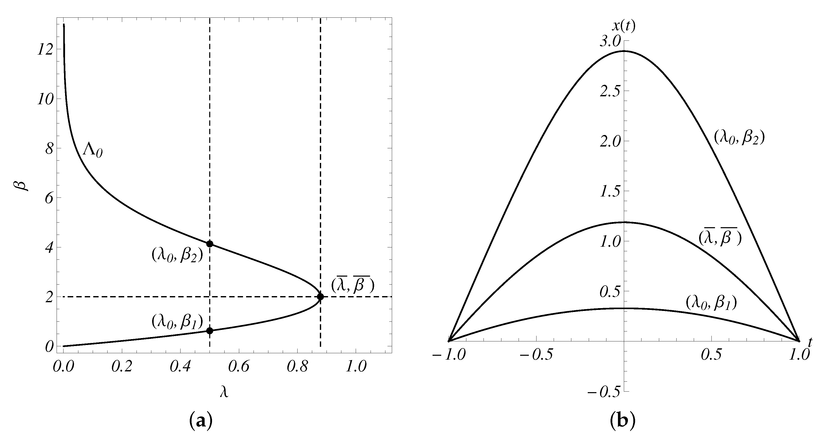
5.2.1. Parameter $\alpha$ Is Zero

If $\alpha =0$, then (11) reduces to the classical one-dimensional Liouville–Gelfand problem; see, for example, [46]:

$$x^{″}+\lambda e^x=0,x(-1)=0,x\left(1\right)=0.$$

(25)

For completeness of the presentation, we will briefly state results on the existence and multiplicity of solutions to (25). Assume that x solves (25). Since $x^{″}\left(t\right)=-\lambda e^{x\left(t\right)}<0$ for every $t\in [-1,1]$, we see that x is strictly concave in $[-1,1]$ and thus x is a positive solution of (25). In view of Proposition 1(3), $x^{\prime }(-1)>0$ and $x^{\prime }\left(1\right)<0$. Moreover, x is an even function in $[-1,1]$—see [47]—and thus $x^{\prime }\left(1\right)=-x^{\prime }(-1)$ and $x^{\prime }\left(0\right)=0$. We infer that the solutions of (25) are in one-to-one correspondence with the ones of

$$x^{″}+\lambda e^x=0,x^{\prime }\left(0\right)=0,x\left(1\right)=0;$$

(26)

the last problem is considered, for example, in ([48], p. 34).

One can show that the initial value problem

$$x^{″}+\lambda e^x=0,x(-1)=0,x^{\prime }(-1)=\beta >0$$

(27)

has a solution

$$x\left(t\right)=ln\left(\frac{{\beta }^2+2\lambda }{B}\right),t\in \mathbb{R},$$

(28)

where

$$B={\left[\sqrt{{\beta }^2+2\lambda }cosh\left(\frac{1}{2}(t+1)\sqrt{{\beta }^2+2\lambda }\right)-\beta sinh\left(\frac{1}{2}(t+1)\sqrt{{\beta }^2+2\lambda }\right)\right]}^2.$$

For x defined by (28), $x\left(1\right)=0$ if and only if $G(\lambda ,\beta ):=\beta -\sqrt{{\beta }^2+2\lambda }tanh\left(\frac{1}{2}\sqrt{{\beta }^2+2\lambda }\right)=0$; see also ([48], p. 34). Let ${\mathrm{\Lambda }}_0:=\left\{(\lambda ,\beta )\in {\mathbb{R}}^2:\lambda >0,\beta >0,G(\lambda ,\beta )=0\right\}$. Since x solves the boundary value problem (25) if and only if there exists $(\lambda ,\beta )\in {\mathrm{\Lambda }}_0$ such that x solves the initial value problem (27), we see that the curve ${\mathrm{\Lambda }}_0$ determines all positive solutions of (25); the curve ${\mathrm{\Lambda }}_0$ is said to be a bifurcation curve for (25). The curve ${\mathrm{\Lambda }}_0$ is a ⊃-shaped curve on the $(\lambda ,\beta )$-plane—see Figure 2a—and ${\mathrm{\Lambda }}_0$ has a turning point $(\overline{\lambda },\overline{\beta })=(0.8785,2.)$ from right to left. Therefore—see ([48], p. 33) and [46]—we come to the following conclusion: the problem (25) has exactly two positive solutions for $\lambda \in (0,\overline{\lambda })$, exactly one positive solution for $\lambda =\overline{\lambda }$ and has no positive solutions for $\lambda >\overline{\lambda }$; see Figure 2.

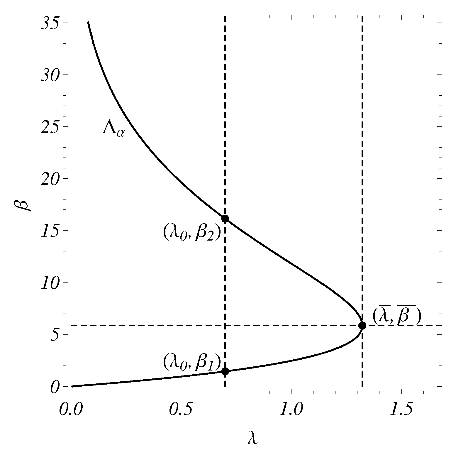
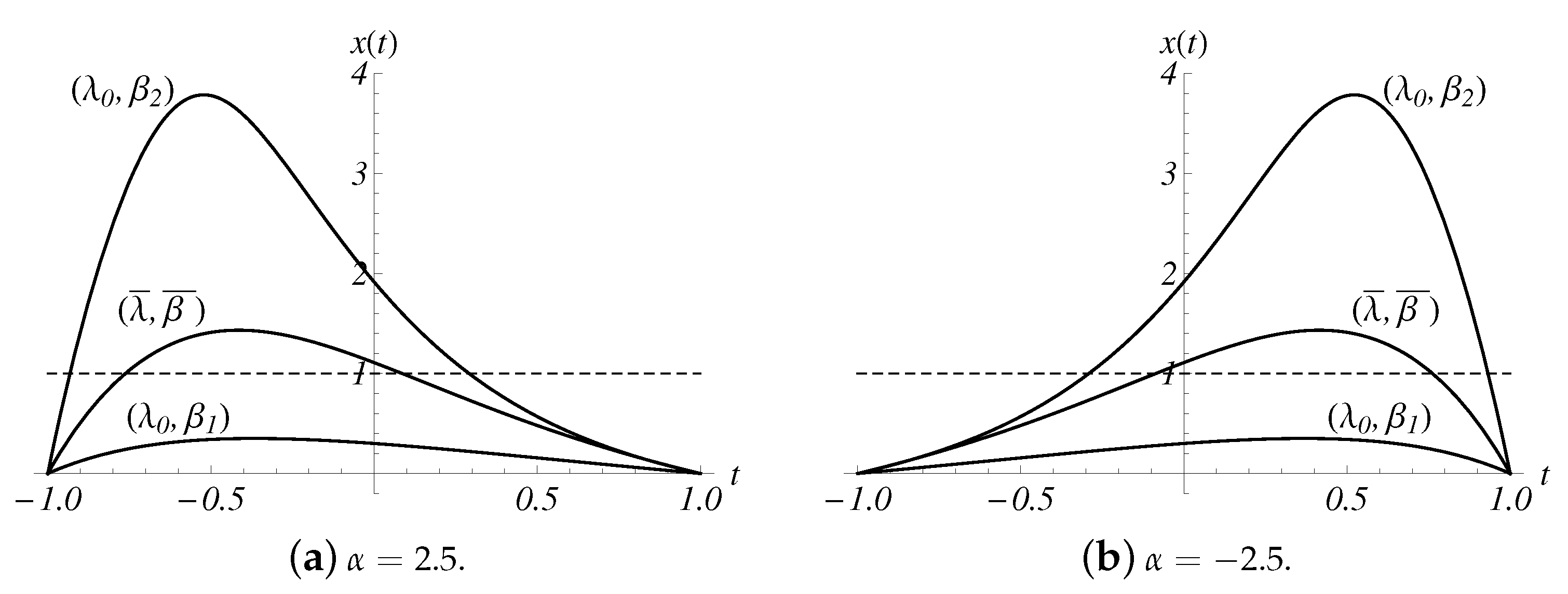
5.2.2. Parameter $\alpha$ Is Nonzero

For a nonzero $\alpha$, we will numerically obtain a bifurcation curve that determines all positive solutions of (11).

Let $\alpha$ be a positive number. Recall that every solution x of (11) is positive—see Corollary 1—and thus $x^{\prime }(-1)>0$ by Proposition 1(3). We will apply the forward shooting method. Suppose that x solves the initial value problem

$$x^{″}+\alpha x^{\prime }+\lambda e^x=0,x(-1)=0,x^{\prime }(-1)=\beta >0;$$

(29)

then, calculate the value $t(\lambda ,\beta )$ such that (a) $t(\lambda ,\beta )>-1$, (b) $x\left(t(\lambda ,\beta )\right)=0$ and (c) $x\left(t\right)>0$ for $-1<t<t(\lambda ,\beta )$. The curve ${\mathrm{\Lambda }}_{\alpha }:=\left\{(\lambda ,\beta )\in {\mathbb{R}}^2:\lambda >0,\beta >0,t(\lambda ,\beta )=1\right\}$ determines all positive solutions of (11) since x solves the boundary value problem (11) if and only if there exists $(\lambda ,\beta )\in {\mathrm{\Lambda }}_{\alpha }$ such that x solves the initial value problem (29); the curve ${\mathrm{\Lambda }}_{\alpha }$ is called a bifurcation curve for (11). Numerical calculations show that ${\mathrm{\Lambda }}_{\alpha }$ is a ⊃-shaped curve on the $(\lambda ,\beta )$-plane; for example, the curve ${\mathrm{\Lambda }}_{\alpha }$ if $\alpha =2.5$ is depicted in Figure 3, and ${\mathrm{\Lambda }}_{\alpha }$ has a turning point $(\overline{\lambda },\overline{\beta })=(1.3224,5.8501)$ from right to left.

Let $\alpha$ be a negative number. In view of Proposition 1(2) and the previous study in this section, the curve ${\mathrm{\Lambda }}_{\left|\alpha \right|}$ determines all positive solutions of (11) since x solves the boundary value problem (11) if and only if there exists $(\lambda ,\beta )\in {\mathrm{\Lambda }}_{\left|\alpha \right|}$ such that x solves the initial value problem $x^{″}+\alpha x^{\prime }+\lambda e^x=0$, $x\left(1\right)=0$, $x^{\prime }\left(1\right)=-\beta$.

Let $\alpha$ be a nonzero number. Since ${\mathrm{\Lambda }}_{\left|\alpha \right|}$ is a ⊃-shaped curve on the $(\lambda ,\beta )$-plane, we arrive at the following conclusion: there exists a positive number $\overline{\lambda }$ such that the problem (11) has exactly two positive solutions for $\lambda \in (0,\overline{\lambda })$, exactly one positive solution for $\lambda =\overline{\lambda }$ and no positive solutions for $\lambda >\overline{\lambda }$; see Figure 3 and Figure 4. Let us calculate ${\lambda }^{*}\left(1\right)$ in accordance with (24). For $\lambda \in \left(0,{\lambda }^{*}\left(1\right)\right)$, the numerical solutions of (11) obtained using the bifurcation curve for (11) confirm the conclusion of Theorem 2. For example, if $\alpha =\pm 2.5$ and $\lambda ={\lambda }_0$, where ${\lambda }_0=0.7$, then $\lambda <{\lambda }^{*}\left(1\right)=0.7495$ and the numerical solutions of (11) corresponding to the points $({\lambda }_0,{\beta }_1)$ and $({\lambda }_0,{\beta }_2)$ on the bifurcation curve ${\mathrm{\Lambda }}_{\left|\alpha \right|}$ are positive and have a norm in the space $C_{[-1,1]}$ less than and more than one, respectively; see Figure 3 and Figure 4.

5.3. Parameter Analysis

Theorem 3. 

If $\lambda \le \frac{3}{2e}=0.5518$, then, for every real number α, the problem (11) has two positive solutions $\underline{x}$ and $\overline{x}$ such that $\parallel \underline{x}\parallel <1<\parallel \overline{x}\parallel$.

Proof. 

Let $\alpha$ be a nonzero real number. In Theorem 2, the value ${\lambda }^{*}\left(1\right)$ depends on $\alpha$:

$${\lambda }^{*}\left(1\right)=\frac{{\alpha }^2}{2e\left(\left|\alpha \right|coth\left|\alpha \right|-1\right)}=:p\left(\alpha \right),\alpha \in \mathbb{R}\setminus \left\{0\right\}.$$

(30)

Since $\underset{\alpha \to 0}{lim}p\left(\alpha \right)=\frac{3}{2e}$, we can extend the function p on the entire real axis by setting $p\left(0\right):=\frac{3}{2e}$. We see that p is a continuous even function on $\mathbb{R}$; the function p is strictly decreasing on the interval $(-\infty ,0)$, and it is strictly increasing on the interval $(0,+\infty )$. We conclude that $p\left(0\right)<p\left(\alpha \right)$ for every nonzero $\alpha$. If $\lambda \le \frac{3}{2e}$, then, in view of (30), we have $\lambda <{\lambda }^{*}\left(1\right)$ and thus the proof follows from Theorem 2.

Suppose that $\alpha =0$. On account of ([48], p. 33), solutions of the boundary value problem (25) or (26) are exactly solutions of the initial value problem

$$x^{″}+\lambda e^x=0,x\left(0\right)=q>0,x^{\prime }\left(0\right)=0$$

(31)

if $\lambda =h\left(q\right)$, where the function $h:(0,+\infty )\to \mathbb{R}$ is defined by $h\left(q\right):=\frac{1}{2}{e}^{-q}{\left[ln\left(\frac{1+\sqrt{1-e^{-q}}}{1-\sqrt{1-e^{-q}}}\right)\right]}^2$. If x solves (31) with $\lambda =h\left(q\right)$, then x solves (25) and the norm $\parallel x\parallel$ in $C_{[-1,1]}$ is equal to q. The function h has the following properties: (a) the function h is continuous; (b) there exists a unique global maximum point $\overline{q}=1.1868$ and $h\left(\overline{q}\right)=\overline{\lambda }$, where $\overline{\lambda }=0.8785$ (the same $\overline{\lambda }$ as in Section 5.2.1); (c) the function h is strictly increasing on the interval $(0,\overline{q})$ and strictly decreasing on the interval $(\overline{q},+\infty )$; (d) $\underset{q\to 0+}{lim}h\left(q\right)=0$, $\underset{q\to +\infty }{lim}h\left(q\right)=0$; (e) $h\left(1\right)=0.8663=h\left(q_1\right)$, where $q_1=1.3952$. Suppose that $\lambda \le \frac{3}{2e}$; then, it follows from (a)–(e) that there exist exactly two positive numbers $\underline{q}$ and $\overline{q}$ such that $\underline{q}<1<\overline{q}$ and $h\left(\underline{q}\right)=\lambda =h\left(\overline{q}\right)$. If $\underline{x}$ and $\overline{x}$ are solutions of (31) with $q=\underline{q}$ and $q=\overline{q}$, respectively, then $\underline{x}$ and $\overline{x}$ are positive solutions of (11) with $\parallel \underline{x}\parallel <1<\parallel \overline{x}\parallel$.    □

6. Linear Stability Analysis

Rather detailed information on the solution of the nonlinear boundary value problem is obtained in the previous sections. As a result, we know that for each $Re$ there exists an interval $0<\lambda <{\lambda }_{*}\left(Re\right)$ such that two steady solutions exist. An example of the two solutions of the base flow temperature distribution is shown in Figure 5 and Figure 6 for $F=0.5$ and three values of the Reynolds number $Re$, namely $Re=0,2$ and 4. Which of the two profiles for each $Re$ should be selected for stability analysis? It is shown in [49] that, for problem (11) without convection, the distribution with higher values of the temperature is linearly unstable with respect to small perturbations for all wave numbers k (and, therefore, is not physically realizable). Calculations for the case $Re=0$ in [21] have shown that the base flow regime with higher temperature is linearly unstable for all Grashof numbers in a certain range of k values. Thus, such a regime is also not physically realizable. Based on the arguments in papers [21,49], we restrict ourselves to the base flow temperature distribution with the smaller norm. The base flow velocity distribution corresponding to the solution shown in Figure 5 is plotted in Figure 7. All linear stability calculations should be performed in the interval $0<\lambda <{\lambda }_{*}\left(Re\right)$.

The numerical solution of problem (7)–(10) is obtained using Matlab routine bvp4c.The base flow temperature distribution becomes more asymmetric as $Re$ increases. Instability is expected since the velocity profiles contain inflection points [10]. However, the velocity gradients at the inflection points decrease as $Re$ increases, indicating a possible stabilization of the base flow for larger $Re$. This observation is supported by linear stability calculations in the next section.

Consider a perturbed flow of the form $\mathbf{v}={\mathbf{v}}_{\mathbf{0}}+{\mathbf{v}}^{\prime }$, $T=T_0+T^{\prime }$ and $p=p_0+p^{\prime }$, where ${\mathbf{v}}^{\prime }$, $T^{\prime }$ and $p^{\prime }$ are small unsteady perturbations. Previous studies for the case of uniform heat generation have shown that plane perturbations are the most unstable for the case of a vertical fluid layer while three-dimensional perturbations are responsible for instability in an inclined fluid layer for a certain range of inclination angles (see [50]). Thus, we assume ${\mathbf{v}}^{\prime }$ in the form: ${\mathbf{v}}^{\prime }=(u^{\prime },0,w^{\prime })$. It is convenient to introduce the stream function ${\psi }^{\prime }$ by the relations

$$u^{\prime }=\frac{\partial {\psi }^{\prime }}{\partial \zeta },w^{\prime }=-\frac{\partial {\psi }^{\prime }}{\partial \xi }.$$

Using a standard linearization procedure (see, for example, [10]), we obtain the system of linear partial differential equations for the unknowns ${\psi }^{\prime }$, $T^{\prime }$ and $p^{\prime }$. We eliminate the pressure perturbation and use the normal modes of the form

$$\begin{array}{ccc}\hfill {\psi }^{\prime }(\xi ,\zeta ,\tau )& =& \phi \left(\xi \right)e^{ik\zeta -\mu \tau },\hfill \\ \hfill T^{\prime }(\xi ,\zeta ,\tau )& =& \theta \left(\xi \right)e^{ik\zeta -\mu \tau },\hfill \end{array}$$

(32)

where k is the wave number and $\mu ={\mu }_r+i{\mu }_i$ is the complex decrement. As a result, the following system of ordinary differential equations for the amplitudes $\phi \left(\xi \right)$ and $\theta \left(\xi \right)$ is obtained:

$$\begin{array}{cc}{\phi }^{\left(4\right)}-2k^2{\phi }^{″}+k^4\phi +ikGr(\phi W_0^{{}^{″}}-W_0{\phi }^{{}^{″}}\hfill & +k^2{W}_0\phi )\hspace{1em}\hspace{1em}\hspace{1em}\hfill \\ & -Re{\phi }^{{}^{‴}}+k^{2}Re{\phi }^{\prime }+{\theta }^{\prime }=-\mu ({\phi }^{{}^{″}}-k^2\phi ),\hfill \end{array}$$

(33)

$$\frac{1}{Pr}({\theta }^{{}^{″}}-k^2\theta )+\frac{\lambda }{Pr}{e}^{T_0}\theta +ikGr(\phi T_0^{\prime }-W_0\theta )-Re{\theta }^{\prime }=-\mu \theta .$$

(34)

The boundary conditions are

$$\phi (\pm 1)=0,{\phi }^{\prime }(\pm 1)=0,\theta (\pm 1)=0.$$

(35)

Problem (33)–(35) is an eigenvalue problem. The base flow is said to be stable if all ${\mu }_r>0$ and unstable if at least one ${\mu }_r<0$.

The numerical solution of (33)–(35) is obtained using the collocation method, where the functions $\phi \left(\xi \right)$ and $\theta \left(\xi \right)$ are approximated as follows:

$$\begin{array}{ccc}\hfill \phi \left(\xi \right)& =& \sum _{m=0}^N{a}_m{(1-{\xi }^2)}^2{T}_m\left(\xi \right),\hfill \end{array}$$

(36)

$$\begin{array}{ccc}\hfill \theta \left(\xi \right)& =& \sum _{m=0}^N{b}_m{(1-{\xi }^2)}^2{T}_m\left(\xi \right),\hfill \end{array}$$

(37)

where $T_m\left(\xi \right)=cosmarccos\left(\xi \right)$ is the Chebyshev polynomial of the first kind of order m. Here, $a_m$ and $b_m$ are unknown coefficients. The collocation points are

$${\xi }_m=cos\frac{m\pi }{N},m=0,1,\dots ,N.$$

(38)

Different numerical methods are available for the solution of (33)–(35). The approximation of the solution is based on Chebyshev polynomials. It is known that if the coefficients of the differential equation are functions from the space $C^{\infty }$; that is, if the coefficients are functions such that the derivatives of all orders exist, then the series in terms of Chebyshev polynomials has an exponential convergence: for large m, the series converges faster than $1/m^s$, where s is any natural number (see [51]). This is the reason why the approximations in the form (36) and (37) are chosen. In addition, it is known that the use of the base functions of the form (36) and (37) satisfying the boundary conditions considerably reduces the condition number of the corresponding matrix after discretization (see [52]).

In order to analyze the numerical convergence of the method, we perform calculations for one set of parameters, namely $k=1.6$, $Re=7$, $F=0.7$ and different number of collocation points N. The results are shown in

Table 1. The values of the Grashof number $Gr$ for different numbers of collocation points N.

N	$\mathbf{Gr}$
30	11,157.351253
40	11,157.569064
50	11,157.811295
60	11,157.624778
70	11,157.625483
80	11,157.625661
90	11,157.649458
100	11,157.639824
110	11,157.650583
120	11,157.640381
130	11,157.632748

. It is known (see, for example, [53]) that the accuracy of the calculation of the Chebyshev collocation derivative is limited. There exists such a value of $N_{*}$ such that the accuracy decreases if $N>N_{*}$. It is seen from Table 1 that one decimal place after the decimal point is correctly calculated for all N considered in Table 1, but a higher accuracy cannot be guaranteed. However, such an accuracy is more than sufficient to represent the results graphically. Similar calculations are performed for other sets of parameters. Calculations show that it is sufficient to use $N=60$ for all cases considered in the paper.

Further verification of the numerical procedure is performed by a comparison of our results with the numerical results presented in [21] for $Re=0$. The results in [21] are shown only in graphical form so that an accurate comparison is technically not possible. It is seen from Figure 2 in [21] that the critical value of the Grashof number for the case $Re=0$, $\lambda =0.75$ is about 1000 (more precise estimate is not possible). Our calculations give $G{r}_c=1014.15$.

7. Numerical Results

Preliminary numerical results of the linear stability analysis are reported in [54] for small values of $Re$. All calculations below are performed for the case $Pr=1$ (a typical value for gases). Three values of the Frank–Kamenetskii parameter $\lambda$ are selected for computations, namely $\lambda =0.3,0.5$ and 0.7. Marginal stability curves for different values of the Reynolds number $Re$ are shown in Figure 8, Figure 9, Figure 10 and Figure 11. The base flow is linearly stable below the marginal stability curve, linearly unstable above it and, on the marginal stability curve, the growth rate of one normal mode is zero while the growth rates of all other modes are negative (all other normal modes are exponentially decreasing with time). Three different colors in Figure 8, Figure 9, Figure 10 and Figure 11 represent calculated values for different $\lambda$ values: red color—for $\lambda =0.3$; green color—for $\lambda =0.5$; and blue color—for $\lambda =0.7$. Calculations are presented for a typical range of the k-values ($0<k<2$). The Grashof numbers on the marginal stability curves in the region $k>2$ usually increase rather rapidly. We also could not find other extrema (at least for the range of the parameters considered in the study) on the marginal stability curves in the region $k>2$. The points on the graphs show the calculated values while solid lines represent spline interpolation of the calculated values.

It is seen from the graphs that the marginal stability curves undergo continuous transformation as the Reynolds number increases. For the case $Re=0$, all marginal stability curves have one minimum (see Figure 8). One or two additional minima in the regions of smaller k appear for the case $Re=5$ as can be seen from Figure 9. As $Re$ increases further (see Figure 10 for $Re=7$), the second minimum still exists, but is gradually moving to the region of larger k. Finally, for $Re=10$ (see Figure 11), the second minimum disappears.

Critical values of the Grashof number $G{r}_c$ versus $Re$ are shown in Figure 12 for three values of $\lambda$. It is seen from the graph that the critical values $G{r}_c$ can be divided into three regions: (1) a region of stabilization ($0<Re<R{e}^{*}$), where $R{e}^{*}$ is approximately equal to 4.791, 4.630 and 4.688 for the values of $\lambda =0.3,0.5$ and 0.7, respectively; (2) a small region (around $Re=5$), where the increase in $Re$ leads to destabilization of the flow; and (3) $6<Re<10$, where the flow is stabilized again. Note that stabilization is stronger for smaller $\lambda$.

Critical wave numbers $k_c$ are plotted versus $Re$ for three values of $\lambda$ in Figure 13, Figure 14 and Figure 15. It is seen from the graphs that there is a finite jump in the critical wave numbers at $Re=R{e}^{*}$. The corresponding marginal stability curve has two equal minima. Thus, at $Re=R{e}^{*}$, there is a transition from one mode with larger k to the other mode with smaller k as $Re$ passes through the point $Re=R{e}^{*}$. A further increase in $Re$ leads to critical perturbations with larger wave numbers.

8. Discussion

The linear stability of a convective flow caused by nonlinear heat sources in a vertical fluid layer is investigated in this paper. It is assumed that the walls of the channel are maintained at constant equal temperatures. In addition, the channel walls are permeable so that there is a flow of constant velocity through the walls of the channel. The problem for the determination of the base flow becomes nonlinear, but the nonlinearity appears only in the heat equation. Thus, the boundary value problem for the base flow temperature can be solved separately. Rigorous mathematical tools such as Krasnosel’skiĭ–Guo cone expansion/contraction theorem are used to analyze the number of solutions depending on the values of the Frank–Kamenetskii parameter and the properties of the solutions. It is shown that, in the region of interest for linear stability analysis, two solutions exist (one with the maximum norm that is smaller than 1 and the other with the maximum norm that is larger than 1). The selection of the “correct” solution for the linear stability analysis is a difficult task. To the best of the authors’ knowledge, there is no theoretically supported recommendation on the selection criteria in the literature. The analysis in [49] for the pure conduction case (no convection) has shown that the solution with a larger norm is linearly unstable with respect to small perturbations. It is shown numerically in [21] that, for the case $Re=0$ and one set of the parameters of the problem, the solution with a larger norm is unstable for all Grashof numbers in a certain range of the wave numbers k. This means that such a solution cannot be observed in experiments. Our approach that selects the solution with the smallest norm is based on the results presented in [21,49]. Future work is required in order to find a theoretical basis for the selection of one solution in cases where a nonlinear boundary value problem has more than one solution.

Linear stability analysis of the base flow is performed numerically using the collocation method based on Chebyshev polynomials. The results are presented in the form of marginal stability curves separating the regions of linear stability and instability. Calculations show that the marginal stability curves undergo a continuous deformation as the intensity of the cross-flow (the Reynolds number) increases. Two minima appear on the marginal stability curves for $Re\approx 5$. A small region of destabilization is found around $Re=5$. As $Re$ increases further, the second minimum of the marginal stability curve disappears and strong stabilization of the flow occurs. It is found that an increase in the Frank–Kamenetskii parameter $\lambda$ destabilizes the flow (and possibly leads to more intensive mixing). It is shown experimentally (see, for example, [55]) that an enhanced mixing of actual fuel flow with air leads to a more efficient conversion process of biomass. Thus, instability is desirable and studies that identify factors enhancing instability can help to create devices for more efficient energy conversion.

Linear stability theory gives the conditions of when and how the given base flow becomes unstable. In order to analyze the development of instability above the threshold, a nonlinear system of equations should be solved numerically. In case the Grashof number is slightly larger than the critical value, amplitude evolution equations can be constructed using the method of multiple scales. This approach is found to be rather useful in applications to Taylor–Couette flows (see, for example, [56]) or to convective flows under non-Boussinesq conditions (see [57]). The authors are currently working on this topic.

References

- Lewandowski, W.M.; Ryms, M.; Kosakowski, W. Thermal biomass conversion: A review. Processes 2020, 8, 516. [Google Scholar] [CrossRef]
- Barmina, I.; Valdmanis, R.; Zake, M. The effects of biomass co-gasification and co-firing on the development of combustion dynamics. Energy 2018, 146, 4–12. [Google Scholar] [CrossRef]
- Barmina, I.; Dzenis, M.; Valdmanis, R.; Zake, M. Thermochemical conversion of microwave pre-treated biomass pellets: Combustion of activated pellets. Chem. Eng. Trans. 2021, 86, 103–108. [Google Scholar]
- Banerjee, A.; Paul, D. Developments and applications of porous medium combustion: A recent review. Energy 2021, 221, 119868. [Google Scholar] [CrossRef]
- Stöcker, M. Biofuels and biomass-to-liquid fuels in the bio-refinery: Catalytic conversion of lignocellulosic biomass using porous materials. Angew. Chem. Int. Ed. 2008, 47, 9200–9211. [Google Scholar] [CrossRef] [PubMed]
- Wronski, S.; Molga, E.; Rudniak, L. Dynamic filtration in biotechnology. Bioprocess Eng. 1989, 4, 99–104. [Google Scholar] [CrossRef]
- Li, N.N.; Fane, A.G.; Ho, W.W.; Matsuura, T. Advanced Membrane Technology and Applications; Wiley: New York, NY, USA, 2011. [Google Scholar]
- Herterich, J.G.; Hu, Q.; Field, R.W.; Vella, D.; Griffiths, I.M. Optimizing the operation of a direct-flow flitration device. J. Eng. Math. 2017, 104, 195–211. [Google Scholar] [CrossRef]
- Luo, Z.; Zhou, J. Thermal conversion of biomass. In Handbook on Climate Change Mitigation; Springer: New York, NY, USA, 2012; pp. 1001–1042. [Google Scholar]
- Drazin, P.G.; Reid, W.H. Hydrodynamic Stability; Cambridge University Press: Cambridge, UK, 2004. [Google Scholar]
- Schmid, P.G.; Henningson, D.S. Stability and Transition in Shear Flows; Springer: New York, NY, USA, 2001. [Google Scholar]
- Hudoba, A.; Molokov, S. Linear stability of buoyant convective flow in a vertical channel with internal heat sources and a transverse magnetic field. Phys. Fluids 2016, 28, 114103. [Google Scholar] [CrossRef]
- Richard, Y. Physics of mantle convection. In Treatise of Geophysics; Elsevier: New York, NY, USA, 2015; Volume 7, pp. 23–71. [Google Scholar]
- Gershuni, G.Z.; Zhukhovitskii, E.M.; Iakimov, A.A. Two kinds of instability of stationary convective motion induced by internal heat sources. J. Appl. Math. Mech. 1973, 37, 544–548. [Google Scholar] [CrossRef]
- Takashima, M. The stability of natural convection in a vertical fluid layer with internal heat generation. J. Phys. Soc. Jpn. 1983, 52, 2364–2370. [Google Scholar] [CrossRef]
- Takashima, M. The stability of natural convection due to internal heat sources in a vertical fluid layer. Fluid Dyn. Res. 1990, 6, 15–23. [Google Scholar]
- Rogers, B.B.; Yao, L.S. The importance of Prandtl number for mixed-convection instability. Trans. ASME C J. Heat Transf. 1993, 115, 482–486. [Google Scholar] [CrossRef]
- Kolyshkin, A.A.; Vaillancourt, R. Stability of internally generated thermal convection in a tall vertical annulus. Can. J. Phys. 1991, 69, 743–748. [Google Scholar] [CrossRef]
- Kolyshkin, A.; Koliskina, V. Stability of a convective flow in a pipe caused by internal heat generation. JP J. Heat Mass Transf. 2018, 15, 515–530. [Google Scholar] [CrossRef]
- Shankar, B.M.; Kumar, J.; Shivakumara, I.S. Stability of mixed convection in a differentially heated vertical fluid layer with internal heat sources. Fluid Dyn. Res. 2019, 51, 055501. [Google Scholar] [CrossRef]
- Eremin, E.A. Stability of steady plane-parallel convective motion of a chemically active medium. Fluid Dyn. 1983, 18, 439–441. [Google Scholar] [CrossRef]
- Iltins, I.; Iltina, M.; Kolyshkin, A.; Koliskina, V. Linear stability of a convective flow in an annulus with a nonlinear heat source. JP J. Heat Mass Transf. 2019, 18, 315–329. [Google Scholar] [CrossRef]
- Gritsans, A.; Koliskina, V.; Kolyshkin, A.; Sadyrbaev, F. Linear stability of a combined convective flow in an annulus. Fluids 2023, 8, 130. [Google Scholar] [CrossRef]
- Zhang, X.; Lei, H.; Zhu, L.; Zhu, X.; Qian, M.; Yadavalli, G.; Wu, J.; Chen, S. Thermal behavior and kineric study for catalytic co-pyrolysis of biomass with plastics. Bioresour. Technol. 2016, 220, 233–238. [Google Scholar] [CrossRef]
- Zhang, X.; Lei, H.; Liu, J.; Bu, Q. Thermal decomposition behavior and kinetics for pyrolysis and catalytic pyrolysis of Douglas fir. RSC Adv. 2018, 8, 2196–2202. [Google Scholar]
- Boussinesq, J. Théory Analytique de la Chaleur; Gauthier-Villars: Paris, France, 1903. [Google Scholar]
- Spiegel, E.A.; Veronis, G. On the Boussinesq approximation for a compressible fluid. Astrophys. J. 1960, 131, 442–447. [Google Scholar] [CrossRef]
- Mihailjan, J.M. A rigorous exposition of the Boussinesq approximation applicable to a thin layer of luid. Astrophys. J. 1962, 136, 1126–1133. [Google Scholar] [CrossRef]
- Gershuni, G.Z.; Zhukhovitskii, E.M. Convective Stability of Incompressible Fluids; Ketter Publications: Jerusalem, Israel, 1976. [Google Scholar]
- Gray, D.D.; Giorgini, A. The validity of the Boussinesq approximation for liquids and gases. Int. J. Heat Mass Transf. 1976, 19, 545–551. [Google Scholar] [CrossRef]
- Barletta, A.; Celli, M.; Rees, D.A.S. The use and misuse of the Oberbeck-Boussinesq approximation. Physics 2023, 5, 298–309. [Google Scholar] [CrossRef]
- Mizerski, K.A. The Oberbeck-Boussinesq approximation, In Foundations of Convection with Density Stratification; Springer: New York, NY, USA, 2021; pp. 21–85. [Google Scholar]
- Mayeli, P.; Sheard, G.J. Buoyancy-driven flows beyond the Boussinesq approximation: A brief review. Int. Commun. Heat Mass Transf. 2021, 125, 105316. [Google Scholar] [CrossRef]
- Frank-Kamenetskii, D.A. Diffusion and Heat Exchange in Chemical Kinetics; Princeton: Princeton, NJ, USA, 1955. [Google Scholar]
- Zeldovich, Y.B.; Barenblatt, G.I.; Librovich, V.B.; Makhviladze, G.M. The Mathematical Theory of Combustion and Explosions; Springer: New York, NY, USA, 1985. [Google Scholar]
- White, D., Jr.; Johns, L.E. The Frank-Kamenetskii transformation. Chem. Eng. Sci. 1987, 42, 1849–1851. [Google Scholar] [CrossRef]
- Ershkov, S.; Prosviryakov, E.; Leshchenko, D. Exact solutions for isobaric inhomogeneous Couette flows of a vertically swirling fluid. J. Appl. Comput. Mech. 2023, 9, 521–528. [Google Scholar]
- Shapeev, V.P.; Sidorov, A.F.; Yanenko, N.N. Methods of Differential Constraints and Its Applications in Gas Dynamics; Nauka: Novosibirsk, Russia, 1984. (In Russian) [Google Scholar]
- El Moutaouakil, L.; Boukendil, M.; Hidki, R.; Charqui, Z.; Zrikem, Z.; Abdelbaki, A. Analytical solution for natural convection of a heat-generating fluid in a vertical rectangular cavity with two pairs of heat source/sink. Therm. Sci. Eng. Prog. 2023, 40, 101738. [Google Scholar] [CrossRef]
- Korobkov, M.V.; Pileckas, K.; Pukhnachov, V.V.; Russo, R. The flux problem for the Navier-Stokes equations. Russ. Math. Surv. 2014, 69, 1065–1122. [Google Scholar] [CrossRef]
- Cabada, A.; Cid, J.Á.; Máquez-Villamarín, B. Computation of Green’s functions for boundary value problems with Mathematica. Appl. Math. Comput. 2012, 219, 1919–1936. [Google Scholar] [CrossRef]
- Infante, G. A short course on positive solutions of systems of ODEs via fixed point index. arXiv 2017, arXiv:1306.4875. [Google Scholar]
- Guo, D.; Lakshmikantham, V. Nonlinear Problems in Abstract Cones; Academic Press, Inc.: Boston, MA, USA, 1988. [Google Scholar]
- Precup, R. Methods in Nonlinear Integral Equations; Kluwer Academic Publishers: Dordrecht, The Netherlands, 2002. [Google Scholar]
- Samuilik, I.; Sadyrbaev, F. On a system without critical points arising in heat conductivity theory. WSEAS Trans. Heat Mass Transf. 2022, 17, 151–160. [Google Scholar] [CrossRef]
- Huang, S.-Y.; Wang, S.-H. Proof of a conjecture for the one-dimensional perturbed Gelfand problem from combustion theory. Arch. Ration. Mech. Anal. 2016, 222, 769–825. [Google Scholar] [CrossRef]
- Korman, P.; Li, Y. Generalized averages for solutions of two-point Dirichlet problems. J. Math. Anal. Appl. 1999, 239, 478–484. [Google Scholar] [CrossRef][Green Version]
- Bebernes, J.; Eberly, D. Mathematical Problems from Combustion Theory; Springer: New York, NY, USA, 1989. [Google Scholar]
- Istratov, A.G.; Librovich, V.B. On the stability of the solutions in the steady theory of a thermal explosion. J. Appl. Math. Mech. 1963, 27, 504–512. [Google Scholar] [CrossRef]
- Gershuni, G.Z.; Zhukhovitskii, E.M.; Yakimov, A.A. On stability of plane-parallel convective motion due to internal heat sources. Int. J. Heat Mass Transf. 1974, 17, 717–726. [Google Scholar] [CrossRef]
- Canuto, C.; Quarteroni, A.; Hussaini, M.Y.; Zang, T.A. Spectral Methods. Evolution to Complex Geometries and Applications to Fluid Dynamics; Springer: New York, NY, USA, 2007. [Google Scholar]
- Heinrichs, W. Improved condition number for spectral methods. Math. Comp. 1989, 53, 103–119. [Google Scholar] [CrossRef]
- Don, W.S.; Solomonoff, A. Accuracy and speed in computing the Chebyshev collocation derivative. SIAM J. Sci. Comp. 1995, 16, 1253–1268. [Google Scholar] [CrossRef]
- Kolyshkin, A.; Koliskina, V. On the stability of the flow in a vertical fluid layer with permeable boundaries caused by a nonlinear heat source. In Proceedings of the 7th International Conference Integrity-Reliability-Failure; Gomes, J.F.S., Meguid, S.A., Eds.; Inegi-Inst Engenharia Mecanica E Gestao Industrial: Porto, Portugal, 2020; pp. 611–612. [Google Scholar]
- Abricka, M.; Barmina, I.; Suzdalenko, V.; Zake, M. Combustion dynamics at biomass thermochemical conversion downstream of integrated gasifier and combustor. In Proceedings of the 12th International Scientific Conference Engineering for Rural Development, Jelgava, Latvia, 23–24 May 2013; pp. 638–642. [Google Scholar]
- Martinand, D.; Serre, E.; Lueptow, R.M. Linear and weakly nonlinear analyses of cylindrical Couette flow with axial and radial flows. J. Fluid Mech. 2017, 824, 438–476. [Google Scholar] [CrossRef]
- Suslov, S.A.; Paolucci, S. Stability of non-Boussinesq convection via the complex Ginzburg-Landau model. Fluid Dyn. Res. 2004, 35, 159–203. [Google Scholar] [CrossRef]