A Predictive Maintenance Strategy for Multi-Component Systems Based on Components’ Remaining Useful Life Prediction

Abstract

Industries increasingly rely on intricate multi-component systems, necessitating efficient maintenance strategies to ensure system reliability and minimize downtime. Predictive maintenance, an emerging approach that utilizes data-driven techniques to forecast and prevent failures, holds significant potential in this regard. This paper presents a predictive maintenance strategy tailored specifically for multi-component systems. In order to accurately anticipate the remaining useful life (RUL) of components, we develop a method that combines data and model fusion based on a particle filtering approach and a degradation distribution model. By integrating degradation data with models, our method outperforms traditional model-based approaches in terms of prediction accuracy. Subsequently, we apply an optimized maintenance model to individual components based on the trigger threshold for RUL. This model determines the most optimal maintenance actions for each component, with the aim of minimizing maintenance costs. Furthermore, we introduce an optimized maintenance strategy that incorporates opportunistic maintenance to further reduce the overall maintenance cost of the system. This strategy leverages predicted RUL information to schedule proactive maintenance actions at the opportune moment, resulting in a significant cost reduction compared to traditional periodic maintenance approaches. To validate the feasibility and effectiveness of our proposed strategy, we utilize experimental data from open-source lithium-ion batteries at the NASA PCoE Center. Through this empirical validation, we provide real-world evidence showcasing the applicability and performance of our strategy in a multi-component system.

1. Introduction

With the rapid advancement of technology and the increasing complexity of industrial systems, the reliance on complex multi-component systems has become prevalent across various industries. The widespread adoption of these sophisticated systems, ranging from electronic equipment systems to lithium battery packs, underscores their pivotal role in driving efficient and reliable operations [1]. However, ensuring optimal functionality and minimizing downtime of these systems have increasingly become cardinal business objectives, given their direct impact on operational efficiency, production capabilities, and financial outcomes. To address these challenges, the development of effective maintenance strategies that ensure system reliability and minimize downtime has become crucial.

Among the different maintenance approaches, predictive maintenance has gained considerable attention for its ability to anticipate and prevent failures by leveraging data-driven techniques. Remaining useful life (RUL) refers to the anticipated continuous operational duration of a system component from the current moment until the occurrence of a failure. The focus of maintenance strategies for multi-component systems is primarily centered on the prediction of each component’s RUL and the optimal maintenance time decision, which is specific to each component. This approach largely hinged on independent life predictions and maintenance decisions for every individual component, with the aim of optimizing their performance and reducing system downtime. However, such a methodology often fails to consider the combined maintenance requirements and strategies at the system level, a shortfall that could result in increased overall maintenance costs. Moreover, traditional approaches to predicting the remaining useful life of components have primarily been based on distribution models [2]. These methods utilize statistical analysis and probability theory to predict the lifetime of components based on their historical failure data. While this approach has been somewhat effective, it does not fully utilize the vast array of data available in the era of Industry 4.0. At present, the application of lithium battery packs is becoming more and more widespread, and their reliability and safety become as important as their performance. Therefore, the study of life prediction and maintenance strategy for multi-component systems composed of multiple batteries is of great significance for the rational arrangement of system maintenance activities as well as the reduction in system maintenance costs. This paper presents a predictive maintenance strategy tailored specifically for multi-component systems. This strategy enables a maintenance plan that minimizes the total maintenance cost based on the degradation state of the components and the correlation between the components.

The main contributions of this paper can be summarized as follows:

(1)

We propose a data and model fusion method for accurately predicting the remaining useful life (RUL) of components in multi-component systems. Our approach utilizes particle filtering to develop an RUL prediction model that continuously updates and refines degradation parameters based on sensor data. This enables more accurate RUL predictions compared to traditional methods.

(2)

Additionally, we introduce an optimized maintenance model aimed at minimizing maintenance costs. By considering RUL thresholds of individual components, our model determines optimal maintenance actions for each component, improving overall system efficiency and cost-effectiveness. Moreover, we address the limitations of focusing solely on individual components by proposing an integrated system-wide maintenance strategy. This strategy incorporates opportunistic maintenance, scheduling proactive actions based on predicted RUL information to significantly reduce total system maintenance costs.

(3)

To validate our strategy, we conducted experiments using open-source lithium-ion batteries at the NASA PCoE Center. The empirical validation provides real-world evidence supporting the effectiveness and applicability of our proposed strategy in multi-component systems.

Overall, this paper makes significant contributions to predictive maintenance in multi-component systems by combining accurate RUL prediction with cost-effective maintenance strategies.

The remainder of this paper is organized as follows: Section 2 provides an overview of related work in the field of predictive maintenance for multi-component systems. Section 3 presents the methodology, including the particle-filtering-based RUL prediction model and the optimized maintenance strategy using opportunity maintenance. Section 4 presents the experimental setup and results. Finally, Section 5 concludes the paper and discusses future research directions.

2. Literature Review

With the advent of Industry 4.0, modern equipment is evolving towards integration, precision, and intelligence. Many of these equipment systems are complex, and composed of multiple components that enhance production efficiency and reduce operational costs. However, the significance of daily maintenance for such equipment systems cannot be overlooked. Certain parts within these systems undergo frequent usage, leading to wear and tear during operation. Moreover, they are susceptible to external environmental factors that contribute to performance degradation and eventual failure. In a study by Minou C.A. Olde Keizer et al. [3], the authors emphasize the importance of considering resource relevance in maintenance decision-making processes. This encompasses aspects such as maintenance personnel availability, tool accessibility, spare parts inventory management, transportation logistics, and budgetary limitations, among others. In comparison to simpler equipment systems with fewer components, multi-component systems pose greater complexity due to their larger number of elements involved. Henceforth, a simplistic approach involving a superposition based on single-component system principles would result in excessive system maintenance cycles that ultimately compromise operational efficiency and escalate company expenses. Consequently, it becomes imperative to investigate the actual degradation trends exhibited by multiple components within a system as well as accurately predict their RUL. With such profound insights at hand, one can orchestrate meticulous maintenance strategies grounded in projected component conditions, all the while upholding stability and safeguarding the integrity of multi-component system operations. RUL prediction serves as a prevalent approach in facilitating maintenance decision-making processes with two main research avenues: degradation model-based approaches and data-driven approaches emphasizing fusion techniques.

The degradation model-based approaches commonly employed in research include physical models, stochastic empirical models, and non-stochastic empirical models. For instance, Hao et al. [4] applied cumulative damage models to analyze the reliability of microelectromechanical systems. Similarly, Wang et al. [5] developed a Weibull distribution model to predict turbine failures in a wind power plant comprising multiple turbines. Data-driven methods have also gained considerable attention in recent studies. Pan Zheng et al. [6] use long short-term memory networks (LSTM) to predict the bearing’s RUL and used the prediction data to study the choice of maintenance strategy, achieving better results. Liu et al. [7] proposed an advanced prediction model based on improved deep adversarial learning (LSTM-GAN), which combines LSTM with a generative adversarial network (GAN) to overcome the limitations of GAN gradient disappearance. This approach effectively predicts machine states and failure types. In the field of life prediction research, there is a prevailing trend towards data and model fusion techniques. Commonly used fusion methods involve Kalman-filter-based and particle-filter-based approaches. Eshwar et al. [8] presented an online fatigue life prediction model based on an extended Kalman filter for civil infrastructure applications, while Guo et al. [9] successfully predicted remaining effective flight cycles for aircraft auxiliary power units. It is important to note that equipment maintenance decision-making and optimization technology plays a crucial role in reliability engineering. Once system RUL prediction is completed, devising a well-planned maintenance program becomes essential to ensure the operational safety and reliability of equipment systems.

According to the sequence of equipment system failure time, maintenance strategy research work from the earliest fault maintenance and preventive maintenance gradually transitions to predictive maintenance. Addressing the problem of monitoring intervals in predictive maintenance, F.C. Gómez de León Hijes et al. [10] show a methodology to determine and manage the Time Interval Between Measurements (TIBeM), dynamically adapting to each machine and each situation. To be more realistic, Yu-Chung Tsao et al. [11] proposed a nonlinear optimization solution procedure to determine the optimal tariff, generation capacity, investment plan, predictive maintenance budget, and insurance level while maximizing the company’s profit. At present, scholars are mainly in accordance with the type of maintenance object classification research; mainly divided into single-component system maintenance and multi-component system maintenance, the study of multi-component system maintenance decision-making needs to take into account the existence of single components. In the study of single-component systems, Chen et al. [12] proposed a fault prediction model utilizing LSTM networks to incorporate the degradation characteristics of the individual equipment components selected. This model determines the optimal maintenance time based on the predicted failure probability, allowing for an informed decision regarding maintenance strategy aimed at achieving impeccable performance of each individual component. Lv et al. [13] aims at developing a fault prediction model, firstly predicting fault severity and fault type simultaneously and subsequently providing a distinguished maintenance strategy for variable faults accordingly, through which the abnormal faults of equipment can be effectively prevented, and machines can be efficiently and economically maintained based on the model’s suggested decisions. Bouabdallaoui et al. [14], on the other hand, developed an auto-encoder-based model specifically tailored for building facility management. This model predicts the probability of future component failure and subsequently guides field staff in conducting failure discrimination to ensure accurate diagnosis before proceeding with necessary maintenance operations. In another study, Orth, P. [15] investigated and evaluated inherent type I and type II errors embedded within control chart models, hidden Markov models, and proportional risk models commonly employed in condition-based maintenance (CBM) decision making. The focus was placed on examining model accuracy and robustness as a foundation for optimizing maintenance decision-making processes.

Huynh, K.T. [16] developed a comprehensive condition-based maintenance strategy and cost model that investigates the number and sizes of cracks in system components, as well as the corresponding system failure/operating states. This model allows for accurate prediction of the mean and probability distribution of the remaining life of the system. Wang, H. [17], on the other hand, proposed a multi-objective group decision-making framework for condition-based maintenance based on the Dempster–Shafer (D–S) evidence theory. The objective was to establish a robust maintenance decision-making framework by defining an index system with quantitative indicators. This approach enables derivation of optimal maintenance decisions and time points while considering multiple objectives. In another study, Lin, L. [18] constructed a multi-objective decision-making model specifically tailored for condition-based overhaul strategies. The primary goals were to minimize maintenance costs and maximize availability. Based on this model, a comprehensive maintenance decision support system was developed integrating data acquisition, processing, and decision-making processes. Vališ, D. [19], meanwhile, harnessed the specific features of Ornstein–Uhlenbeck processes and Wiener positive drift processes to effectively model operating times and calendar times. By estimating soft failures within systems and determining their remaining technical life, Vališ aimed to optimize planned preventive maintenance strategies. Overall, these studies contribute to advancing our understanding of condition-based maintenance decision making through innovative models that consider multiple factors such as crack sizes, system failure state probabilities, multi-objective optimization approaches based on evidence theory, or overhauling considerations integrated with comprehensive data analysis frameworks.

For multi-component systems, Zhang et al. [20] investigated the degradation correlation between auxiliary and critical components as well as the dynamically changing importance of these components. They introduced a preventive maintenance strategy aimed at minimizing long-term average costs. Specifically, they focused on a two-component system comprising an auxiliary component and a critical component. In a similar vein, Sheikhalishahi et al. [21] proposed a novel maintenance planning method that considered grouping strategies and human factors. Their approach incorporated the understanding that different factors may influence maintenance decisions, leading to more effective planning. Continuing with the theme of maintenance grouping strategies for multi-component systems, Do et al. [22,23,24,25] conducted a series of studies in this area. These studies aimed to optimize maintenance activities by exploring various grouping approaches tailored to specific system requirements. De Pater et al. [26], on the other hand, applied particle-filtering-based number-mode fusion methods for the lifetime prediction of components in an aircraft’s auxiliary cooling system. Subsequently, they developed an integer linear programming model executed on a rolling basis over time. This model effectively predicts which components need maintenance on a daily basis for future periods. Alhourani et al. [27] proposed an efficient preventive maintenance strategy based on calculating equipment reliability following an exponentially distributed distribution. Their approach considered grouping machines with similar failure modes and reliability levels for optimal resource allocation during maintenance operations. Shifting focus toward machine learning approaches in the field of maintenance, Carvalho et al. [28] provided a comprehensive review of current preferred methods such as random forests, artificial neural networks (ANN), convolutional neural networks (CNN), LSTM, support vector machines (SVM), and k-means algorithms. On this basis, Chang [29] proposed a service-oriented dynamic multi-level predictive maintenance grouping strategy. By utilizing k-means clustering, this strategy addressed the optimization problem of grouping at different levels, including the component level, dynamic grouping level, and system level for individual optimization. Gorenstein and Ariel [30] proposed a maintenance model that considers the replacement cost of components, the probability of failure, and the adjacency of replaced components.

In conclusion, although researchers have been dedicated to studying the prediction of remaining service life and maintenance of equipment systems, the traditional approach of relying solely on degradation models for component failure judgment lacks accuracy and efficiency in making decisions regarding multi-component maintenance. Hence, there is a significant practical value in combining monitoring data with degradation models to predict the remaining service life of components and constructing tailored maintenance models. This study utilizes a double exponential degradation model and integrates real-time sensor data with the particle filtering algorithm to achieve more precise predictions of the battery component’s remaining service life. Furthermore, it identifies the optimal moment for maintenance for each component based on this model in real time. Taking into account both economic relevance and opportunity-based maintenance factors within the system, this research calculates the ideal moment for overall system maintenance and determines when precisely multiple components should undergo maintenance operations. Experimental results demonstrate that utilizing this proposed maintenance strategy effectively reduces the overall system maintenance cost rate.

In contrast to similar research methodologies, our approach distinguishes itself through its utilization of a model-based particle filtering technique for prognostication. This enables us to incorporate real-time inspection data in a more authentic manner during the life prediction process, thus enhancing the accuracy and realism of our results. When it comes to maintenance decision making, we adopt an opportunistic maintenance strategy to circumvent unnecessary repairs that may arise from rigid maintenance programs. By doing so, we effectively mitigate maintenance costs and achieve a lower overall expenditure in comparison to alternative methods.

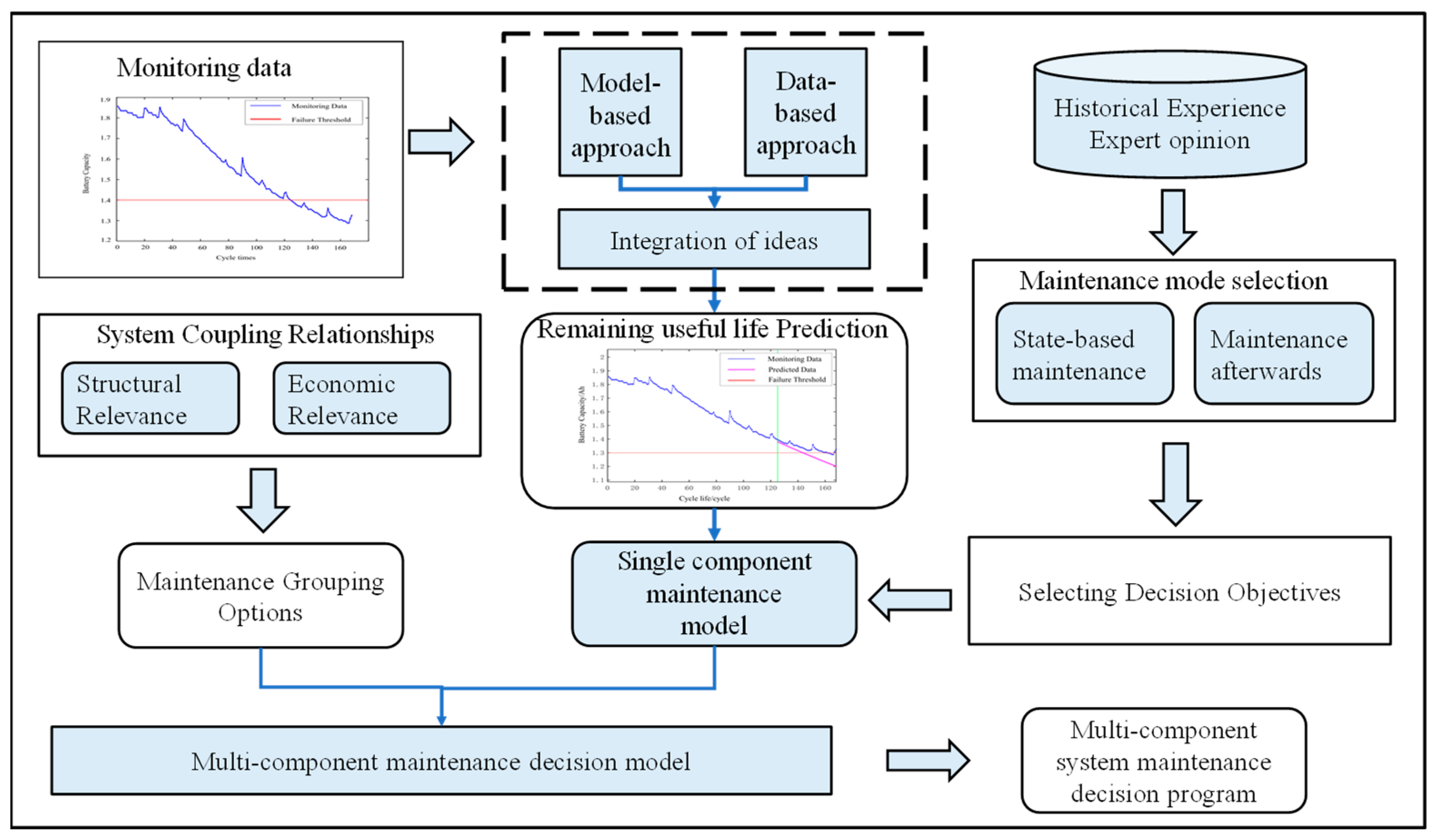
3. Framework of the Proposed System

Before formulating a predictive maintenance strategy for a multi-component system, it is necessary to establish certain assumptions:

(1)

The system under consideration comprises one independent component, where the failure of one component does not affect the reliability of others.

(2)

External environmental factors are disregarded during system operation analysis. Specifically, we focus solely on two distinct maintenance activities: preventive replacement and failure replacement. Following any maintenance intervention, the condition of the respective component immediately reverts to brand new status with a perfect restoration effect.

(3)

Economic considerations come into play when evaluating maintenance strategies for multi-component systems. The cost associated with the simultaneous maintenance of different components is not merely an accumulation of individual component costs. In this study, each instance of maintenance results in system downtime and incurs a fixed configuration cost denoted as S. This cost includes lost production due to downtime, utility expenses, and preparation costs related to setting up overhaul equipment [31]. Importantly, S is independent of the maintenance cost associated with any specific component. Moreover, if opportunistic maintenance is carried out whereby some components are replaced prematurely at the expense of their remaining useful life, additional losses may arise as a consequence.

Based on the aforementioned assumptions, this study has developed the following refined framework for predictive maintenance strategies in multi-component systems:

(1)

To accurately predict the remaining service life of components, a sophisticated approach combining number–model fusion and particle filtering theory is implemented. This method leverages actual monitoring data to model component degradation and estimate the failure probabilities. The optimal moment for maintenance, denoted as $t_R^{\ast }$, is determined by selecting the more cost-efficient option between preventive and non-preventive replacement costs based on the predicted probability of component failure.

(2)

It is assumed that maintenance execution time is minimal, resulting in instantaneous actions. Any downtime experienced during maintenance can be quantified as a fixed configuration cost S, encompassing utility expenses, lost production opportunities, and overhaul-related expenditures. Thus, each instance of maintenance incurs this fixed configuration cost S. On the other hand, preventive replacement costs $C_p$ encompass all expenses associated with proactive maintenance measures such as component replacements, spare parts inventory management, and reservation expenses.

(3)

Recognizing that sudden component failures can lead to undesirable system downtime consequences, emphasis is placed on avoiding such scenarios through proactive preventive replacement actions. If preventive replacement is not carried out at some future time point t, implying an increased risk of component failure, conducting an assessment of expected costs associated with not opting for preventive replacement becomes necessary. This evaluation encompasses both failure replacement costs and potential financial losses due to the unavailability of spare parts.

(4)

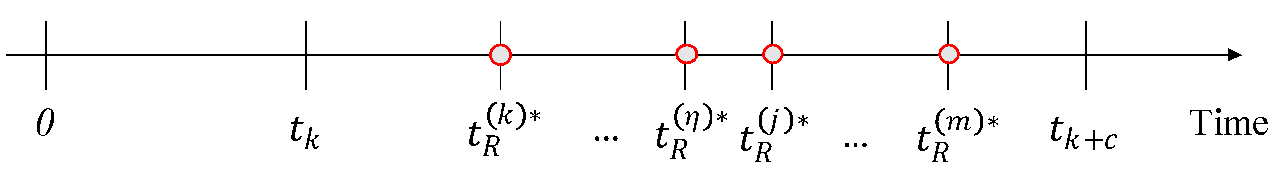
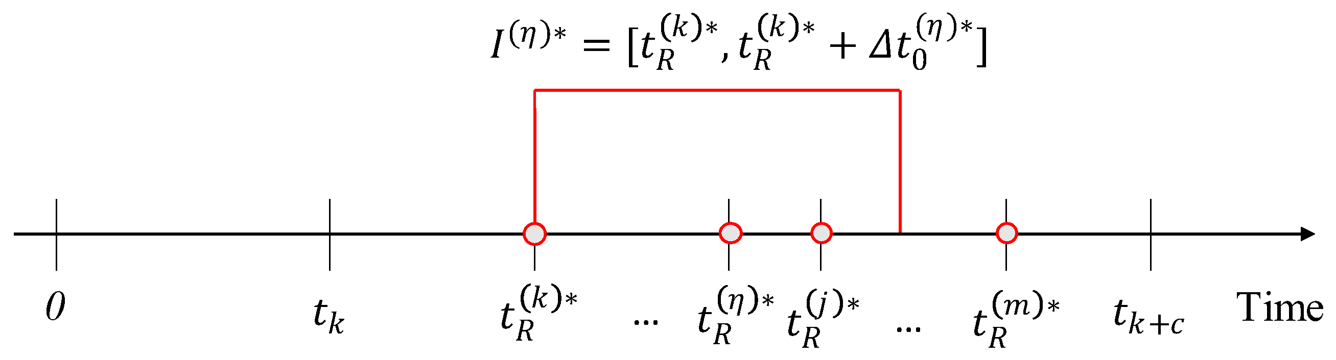
During the maintenance process of a single component within a multi-component system, there exists an opportunity to perform additional maintenance on other components while the entire system comes to a halt temporarily. For instance, when maintaining component k at its optimal moment $t_R^{\left(k\right)\ast }$, if there exists another component η whose optimal moment falls within the interval $t_R^{\left(\eta \right)\ast }\in \left[t_R^{\left(k\right)\ast },t_R^{\left(k\right)\ast }+\mathsf{\Delta }{t}_0^{\left(\eta \right)\ast }\right]$, an opportunity for maintenance on component η at the system level arises. Here, $\mathsf{\Delta }{t}_0^{\left(\eta \right)\ast }$ represents the time threshold at which minimizing setup costs S can be achieved, consequently reducing the overall maintenance cost of the system.

(5)

The combination of components for opportunity maintenance in a multi-component system can be organized into a grouping structure. Each part’s preventive replacement cost within this opportunity maintenance grouping remains as $C_p$, but certain parts may have their service life partially wasted due to earlier maintenance moments, resulting in increased penalty costs denoted as $C_h$, per unit time. By quantifying cost savings, we determine the optimal maintenance grouping.

As depicted in Figure 1, the primary procedure for optimizing the maintenance strategy of a multi-component system unfolds as follows: initially, we acquire signals from sensors (such as vibration signals of bearings or impedance measurements of lithium batteries) that effectively characterize the degradation of each component. Subsequently, through RUL prediction, we derive degradation curves for these components. We then determine the optimal maintenance time for each component by leveraging the maintenance model for single-component systems. Ultimately, by employing a computerized maintenance time window, we formulate the ultimate maintenance plan.

For ease of reference, we present the key symbols that appear in this paper in

Table 1. Symbol List.

Symbolic	Meaning
$C_p$	Single preventive replacement cost
$S$	Single maintenance fixed configuration cost
$C_c$	Sum of single-failure replacement cost and spare parts out-of-stock cost
$C_h$	Penalty Costs
$P_h^{fail}$	Probability of failure of a single component at moment h
$t_R^{\ast }$	The best time to maintain a single part
$t_k$	Current monitoring moments
$MC{R}^{\eta }$	Maintenance cost rate of component η
$\Delta t_0^{\left(\eta \right)\ast }$	Component η optimal opportunity maintenance time window threshold
$c_{os}$	System maintenance cost rate considering opportunity maintenance
$q$	Cost saving rate
$v$	Number of parts that can be executed for maintenance
$G_u$	A collection of parts that can be maintained by execution opportunities

.

3.1. RUL Prediction Based on Particle Filtering Algorithm

The particle filtering algorithm is based on the Monte Carlo method to accomplish the approximate solution of the state probability; the particles represent the different sampling values $\left\{x_{0:k}^i,i=1,2,3,\dots N\right\}$, N is the number of particles (samples), the particle weights represent the normalized weights of the different sampling values $\left\{w_k^i,i=1,2,3,\dots N\right\}$, and particle filtering uses a combination of both to represent the state posterior probability distribution [9]:

$$p\left(x_{0:k}|y_{1:k}\right)\approx {\displaystyle {\displaystyle \sum }_{i=1}^N}{w}_k^i\delta \left(x_{0:k}-x_{0:k}^i\right)$$

(1)

where $\delta \left(\ast \right)$ is the Dirac function, and $\delta \left(x_{0:k}-x_{0:k}^i\right)$ = 1 when $x_{0:k}=x_{0:k}^i$, otherwise $\delta \left(x_{0:k}-x_{0:k}^i\right)$ = 0.

Analysis of the above equation shows that we can find the approximation of the state probability distribution by simply obtaining the distribution of the weights corresponding to the particles. In practical applications, it is very difficult to sample directly in $p\left(x_{0:k}|y_{1:k}\right)$, and an important density function $q\left(x_{0:k}|y_{1:k}\right)$ is usually chosen to complete the sampling instead. Assuming that $q\left(x_{0:k}|y_{1:k}\right)$ represents the posterior probability estimate of the state of the system at different moments of the state, and that the system state and the observed information follow a first-order Markov process (the state of the system at moment $k$ is affected only by the probability of the state at moment $k$ − 1 and is independent of the state at all previous moments), then:

$$w_k^i\propto w_{k-1}^{i}p\left(y_k|x_k^i\right)$$

(2)

Then, the posterior probability density distribution can be approximated as

$$p\left(x_k|y_{1:k}\right)\approx {\displaystyle {\displaystyle \sum }_{i=1}^N}{w}_k^i\delta \left(x_k-x_k^i\right)$$

(3)

After several steps of iterative operations, the problem of particle degeneracy occurs: a small number of particles have higher weights, while most of them have lower weights. To solve this problem and reduce the rate of particle degradation, a resampling step is usually added in the process of algorithm usage. The basic idea of resampling is to copy the particles with higher weights, eliminate the particles with lower weights, and assign the weights of all particles to 1/N, so that the distribution of particles is closer to the real situation. The sampling process of resampling is shown in Figure 2.

In what follows, the residual life prediction data obtained by the LSTM model will be used to quantify the health status of the bearing.

Although resampling can reduce the speed of particle degradation, there is also a disadvantage: it reduces the diversity of particles. Therefore, in the practical application of the algorithm, an effective sampling scale is invoked to determine the number of effective particles, which is defined as

$$N_{eff}=\frac{1}{{{\displaystyle \sum }}_{i=1}^N{(w_k^i)}^2}$$

(4)

where $N_{eff}$ is the number of effective particles, $N_{eff}$ is usually compared with a pre-set threshold $N_{th}$, and resampling is performed when $N_{eff}$ < $N_{th}$, often taking $N_{th}$ = 2N/3.

The flow of particle filtering algorithm implementation is shown in Figure 3, and the steps are as follows:

(1)

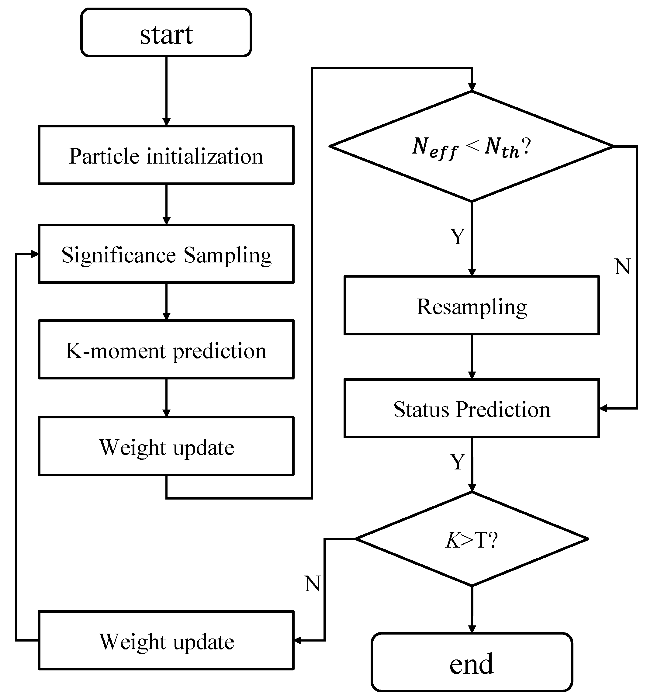
Initialization: at the moment $k=0$, the set of particles ${\left\{x_0^i\right\}}_{i=1}^N$ is generated from the known a priori probability of the system state, $p\left(x_0\right)$, and the initial weights of all the particles are all $1/N$.

(2)

Importance sampling and weights calculation: at the moment k > 0, according to $x_k^i~p\left(x_k|x_{k-1}^i\right)$, the particle weights can be updated as $w_k^i=w_{k-1}^i(p\left(y_k|x_k^i\right)$, where $i=1,2\dots ,N$, and the weights are normalized ${\tilde{w}}_k^i=w_k^i/{\displaystyle \sum }_{i=1}^N{w}_k^i$.

(3)

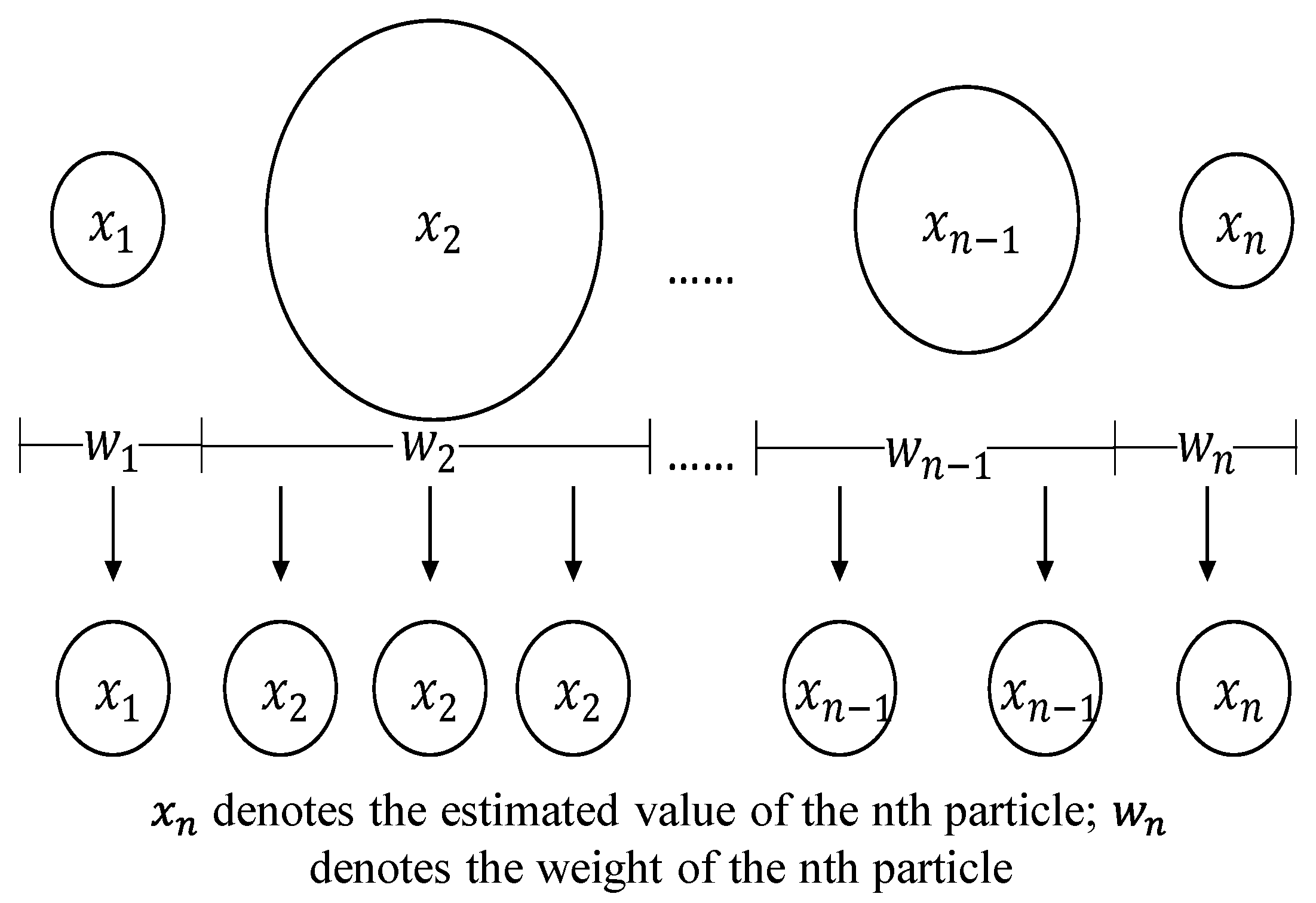
Resampling: according to the effective sampling scale of resampling $N_{eff}$ and preset $N_{th}$ to determine whether to resample combined with the weights obtained in (2), copy the particles with larger weights and eliminate the particles with smaller weights to obtain the new set of particles ${\left\{x_{0:k}^i\right\}}_{i=1}^N$; the weights of each particle are all $1/N$.

(4)

Output state estimate: ${\widehat{x}}_k={\displaystyle \sum }_{i=1}^N{w}_k^i{\tilde{x}}_k^i$.

(5)

Judge the number of times the algorithm is executed: if $k>T$ ($T$ is the number of known observations), exit this algorithm; otherwise, $k=k+1$ and return to (2).

Numerous studies [29] proved that the double exponential degradation model can describe the decay process of battery capacity more accurately, so this paper uses the double exponential degradation model to characterize the battery capacity degradation as follows:

$$C_k=a exp(bk)+c exp(dk)$$

(5)

where $k$ is the current cycle position, $C_k$ is the current capacity estimate, and $a, b, c, d$ are the model parameters, which need to be filtered by us for estimation. We choose the first 125 data points as the experimentally known data, $k$ = 125 is chosen as the starting point for prediction, and the curve is fitted to the first 125 data points by the MATLAB 2020B fitting tool; the individual fitted parameters are shown in

Table 2. Curve fitting parameters.

Parameters	$\mathit{a}$	$\mathit{b}$	$\mathit{c}$	$\mathit{d}$	RMSE	R2
Value	2.0750	−0.0033	−0.2613	−0.0420	0.0194	0.9837

.

We know that when the value of R² is closer to 0 and the value of RMSE is closer to 1, the better the fit is, as we can see from Table 2, R² = 0.0194, RMSE = 0.9837, which indicates that our model fits well.

After determining the degradation model, we use the particle filtering algorithm to complete the estimation of the parameters in the degradation model and then achieve the prediction of the component RUL, and the equation [29] of state at moment $k$ is

$$x_k=\left[a_k,b_k,c_k,d_k\right]$$

(6)

$$\left\{\begin{array}{c}{a}_k=a_{k-1}+w_a w_a~N\left(0,{\sigma }_a\right)\\ b_k=b_{k-1}+w_b w_b~N\left(0,{\sigma }_b\right)\\ c_k=c_{k-1}+w_c w_c~N\left(0,{\sigma }_c\right)\\ d_k=d_{k-1}+w_d w_d~N\left(0,{\sigma }_d\right)\end{array}\right.$$

(7)

The observation equation is given by

$$C_k=a_k exp(b_{k}k)+c_k exp(d_{k}k)+v_k v_k~N\left(0,{\sigma }_v\right)$$

(8)

where $a_k, b_k, c_k, d_k$ are the unknown parameters at moment $k$. $w_a, w_b, w_c, w_d$ are the system state transfer errors. $v_k$ is the systematic observation error.

The definition of component RUL $z_k$ is expressed as

$$RUL= inf\{z_k:C\left(k+z_k\right)\le D\}$$

(9)

where D is the preset life threshold, $z_k$ is the predicted value of the remaining useful life at the current kth moment, and $C\left(k+z_k\right)$ denotes the predicted component degradation level at the $k+z_k$ moment.

We take battery #1 as an example; assuming that the starting moment of the remaining service life prediction of the component is the monitored number of current use cycles, denoted as the kth cycle, its remaining service life prediction steps are as follows:

(1)

Determine the initial parameters $a, b, c, d$ of the degradation model using the MATLAB data fitting tool;

(2)

Execute the particle filtering algorithm using the parameters obtained from 1) and the degradation data monitored by the sensors (battery capacity data from installation to use up to the $k$th cycle) to update the particle set $\left\{x_k^i={\left(a_k^i,b_k^i,c_k^i,d_k^i\right)}^T,w_k^i\right\}$ in real time, where $i=1,2,\dots ,N,$ and $k=1,2,\dots ,k$.

(3)

Applying the particle filtering algorithm in (2), we update the model parameters at different cycle periods until we reach the $k$th cycle, at which point the predicted value of the battery capacity of the ith particle at the kth cycle forward $z_k$ steps is calculated as follows:

$$C_{k+z_k}^i=a_k^i exp[b_k^i\left(k+z_k\right)\left]+c_k^i exp[d_k^i\left(k+z_k\right)\right]$$

(10)

(4)

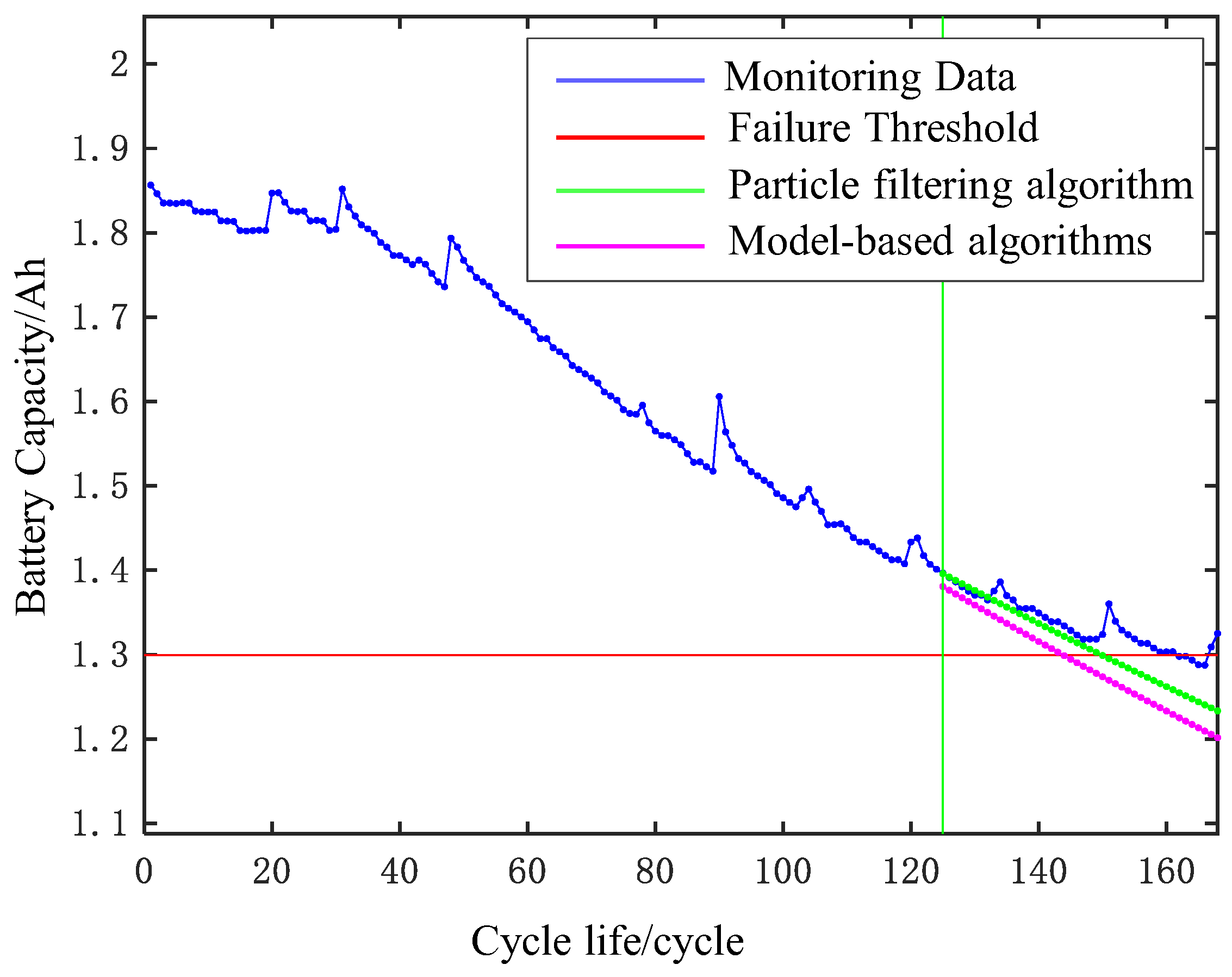
From Equation (9), the battery RUL is the number of cycles from the current number of cycles to the first time the battery reaches its life threshold, assuming a life threshold of 0.72 Ah; then, we calculate the estimate of the RUL of the ith particle at the $k$th cycle:

$$z_k^i= inf\{z_k^i:C_{k+z_k}^i\le 0.72 \mathrm{Ah}\}$$

(11)

The distribution of RUL at the $k$th cycle is approximated according to Equation (3) as

$$p\left(z_k|C_{0:k}\right)\approx {\displaystyle \sum }_{i=1}^N{w}_k^i\delta \left(z_k-z_k^i\right)$$

(12)

Then, the estimate of RUL at the $k$th cycle is

$$z_k\approx {\displaystyle \sum }_{i=1}^N{w}_k^i{z}_k^i$$

(13)

We can obtain the probability density function of RUL for the current kth cycle of the battery component by Equation (12). To assess the component reliability, we define the probability of failure of the battery component before the $h\left(h>k\right)$th cycle in the future as

$$P_h^{fail}=P\left(RUL\le \left(h-k\right)\right)$$

(14)

3.2. Single Component Maintenance Model

The specific decision idea of the optimal maintenance moment for a single component is as follows:

(1)

If we perform preventive replacement maintenance operation at some future h moment, the total cost of performing maintenance is denoted as $\left(C_p+S\right)$, where $C_p$ denotes the preventive replacement cost and $S$ denotes the fixed configuration cost incurred for each performed maintenance.

(2)

If we do not consider performing preventive replacement in the future h moments, the system will not bear the preventive replacement cost from the current moment to the future h moments, but there is a risk of failure due to sudden failure of internal components at h moments and in the subsequent period, in which case we must consider the occurrence of non-preventive replacement operations, and we denote the expected cost of non-preventive replacement as $\left(C_c+S\right)P_h^{fail}$, which includes the replacement cost due to unexpectedly caused sudden failures. The fixed configuration cost $P_h^{fail}$ denotes the predicted probability of failure of the obtained component at moment h, $C_c$ denotes the sum of the failure replacement cost and the spare parts out-of-stock cost, and $S$ denotes the fixed configuration cost.

For a single component, preventive maintenance should be taken if the expected cost of performing preventive replacement is lower or equal to the expected cost of non-preventive replacement, i.e., ($C_p+S)\le \left(C_c+S\right)P_h^{fail}$. Thus, the single-component optimal maintenance moment $t_R^{\ast }$ can be defined as

$$t_R^{\ast }=\underset{h=k+1,k+2,\dots }{inf}\left\{h:|\left(C_p+S\right)\le \left(C_c+S\right)P_h^{fail}\right\}$$

(15)

According to the above equation, the maintenance best maintenance moment for different single components can be found, as shown in Figure 4, where $t_k$ is indicated as the current monitoring moment corresponding to the prediction starting point in part B, $t_{k+c}$ indicates the prediction cutoff moment, and $t_R^{\left(k\right)\ast }, t_R^{\left(\eta \right)\ast }, t_R^{\left(j\right)\ast }, t_R^{\left(m\right)\ast }$ indicate the predicted obtained components $k, \eta , j, m$ at their respective optimal maintenance moments.

In order to assess the effectiveness of maintenance strategies, it is crucial to consider the maintenance cost rate (MCR) associated with each component. The MCR is defined as the ratio between the total maintenance cost and the life cycle of the component [32]. Strategies that yield a lower MCR are deemed more successful in their performance.

In real-world production scenarios, two distinct maintenance situations arise over time:

(1)

If the predicted moment for executing maintenance based on our strategy precedes the actual failure moment of a part, preventive replacement activities can be carried out. In such cases, spare parts are readily available as they have been scheduled in advance. The MCR for this part η can be calculated using the following equation:

$$MC{R}_p^{\eta }=\frac{C_p+S}{t_R^{\left(\eta \right)\ast }}$$

(16)

(2)

If the actual moment of failure of the part is earlier than the predictive maintenance moment (which rarely happens because it would imply a large error in the prediction), then the failure replacement maintenance activity must be performed immediately for the part, in which case the non-preventive replacement cost must be paid because no spare parts are scheduled. In this case, the maintenance cost rate of the component is given by the following equation:

$$MC{R}_c^{\eta }=\frac{C_c+S}{T_F}$$

(17)

where $T_F$ denotes the actual moment of failure of the component.

3.3. Opportunity Maintenance Cost Model

By the method mentioned above, we can obtain the optimal maintenance moment $t_R^{\left(\eta \right)\ast }$ for any component $\eta$ in a multi-part system; the preventive replacement cost is $C_p^{\left(\eta \right)\ast }$, and we assume that the actual maintenance moments of each component are their respective optimal maintenance moments, i.e., without considering opportunity maintenance, the system maintenance cost is the cumulative sum of the preventive replacement cost and the configuration cost of each component:

$$C_s={\displaystyle \sum }_{\eta =1}^l\left[C_p^{\left(\eta \right)\ast }+S\right]$$

(18)

The system maintenance cost rate—the cumulative sum of the maintenance cost per unit of usage time of each component—can be calculated as

$$c_s={\displaystyle \sum }_{\eta =1}^{l}MC{R}_p={\displaystyle \sum }_{\eta =1}^l\frac{C_p^{\left(\eta \right)\ast }+S}{t_R^{\left(\eta \right)\ast }}$$

(19)

Our maintenance strategy model has pointed out that based on the predicted information of the remaining useful life of different components, it is possible to reduce the system maintenance cost by maintaining different components at the same time; however, we have to trade off the penalty cost due to component RUL waste against the fixed configuration cost.

We assume that maintenance is performed simultaneously at $t_R^{\left(k\right)\ast }$ for $v\left(v\le l\right)$ components in the system. $t_R^{\left(k\right)\ast }$ is the best maintenance moment for component $k$ obtained from the prediction and is the best opportunity maintenance moment for the other components. We introduce the concept of penalty cost $C_h^{\left(\eta \right)}$, which denotes the additional cost incurred by advancing the maintenance time of component $\eta$ from its optimal maintenance moment $t_R^{\left(\eta \right)\ast }$ to $t_R^{\left(k\right)\ast }$ resulting in a wasted RUL, and the penalty cost $C_h^{\left(\eta \right)}$ contains the following parameters:

(1)

The optimal maintenance moment $t_R^{\left(\eta \right)\ast }$ of the component $\eta$;

(2)

The moment of opportunity maintenance $t_R^{\left(k\right)\ast }$ of the system;

(3)

The penalty cost per unit time $c_h^{\left(\eta \right)}$ of the component η.

Based on the above parameters, we give the expression for the penalty cost $C_h^{\left(\eta \right)}$ as

$$C_h^{\left(\eta \right)}=c_h^{\left(\eta \right)}\left(t_R^{\left(\eta \right)\ast }-t_R^{\left(k\right)\ast }\right)=c_h^{\left(\eta \right)}\mathsf{\Delta }{t}_R^{\left(\eta \right)}$$

(20)

In this way, we can calculate the cost Q of the predicted opportunity maintenance savings of execution against the component’s RUL:

$$Q=\left(v-1\right)S-{\displaystyle \sum }_{\eta =1}^v{c}_h^{\left(\eta \right)}\left(t_R^{\left(\eta \right)\ast }-t_R^{\left(k\right)\ast }\right)$$

(21)

The cost savings rate is calculated as:

$$q=\frac{Q}{t_R^{\left(k\right)\ast }}=\frac{\left\{\left(v-1\right)S-{{\displaystyle \sum }}_{\eta =1}^v{c}_h^{\left(\eta \right)}\left(t_R^{\left(\eta \right)\ast }-t_R^{\left(k\right)\ast }\right)\right\}}{t_R^{\left(k\right)\ast }}$$

(22)

At this point, the system maintenance cost rate can be calculated as

$$c_{os}=\frac{{{\displaystyle \sum }}_{\eta =1}^v[C_p^{\left(\eta \right)\ast }+S]-Q}{t_R^{\left(k\right)\ast }}+{\displaystyle \sum }_{\eta =1}^{l-v}MC{R}_p$$

(23)

From the above analysis, it can be seen that if all maintenance costs are known, the maintenance cost savings depend on the dynamic opportunity maintenance time window threshold $\mathsf{\Delta }{t}_0^{\left(\eta \right)\ast }$. If the threshold is too small, different components cannot be opportunity maintained at the same time, which will lead to frequent system downtime for maintenance and expenditure of multiple fixed configuration costs; if the threshold is too large, some components are opportunity maintained leading to too many wasted RULs and higher penalty costs. To minimize the total maintenance cost, the fixed configuration cost saved by implementing an opportunity maintenance strategy must be greater than the additional penalty cost paid for wasted component RULs. To achieve this goal, this study sets an optimal opportunity maintenance time window threshold $\mathsf{\Delta }{t}_0^{\left(\eta \right)\ast }$:

$$S=c_h^{\left(\eta \right)}\mathsf{\Delta }{t}_0^{\left(\eta \right)\ast }$$

(24)

The optimal opportunity maintenance time window for component $\eta$ is $I^{\left(\eta \right)\ast }=\left[t_R^{\left(k\right)\ast },t_R^{\left(k\right)\ast }+\mathsf{\Delta }{t}_0^{\left(\eta \right)\ast }\right]$, as shown in Figure 5. When the best maintenance moment $t_R^{\left(\eta \right)\ast }\in \left[t_R^{\left(k\right)\ast },t_R^{\left(k\right)\ast }+\mathsf{\Delta }{t}_0^{\left(\eta \right)\ast }\right]$, the difference between the best maintenance moments of two components $\mathsf{\Delta }{t}_R^{\left(\eta \right)}\le \mathsf{\Delta }{t}_0^{\left(\eta \right)\ast }$, which means that it can be performed at the system opportunity maintenance moment $t_R^{\left(k\right)\ast }$ for the other components located in the respective opportunity maintenance time window. All components performing opportunity maintenance are considered as a grouped structure $G_u$ that dynamically adjusts according to the prediction information, i.e., $G_u$ consists of all components within the system with different attributes but performing maintenance at the same moment.

Although the opportunistic maintenance strategy is not sufficiently resistant to sudden disturbances, the correct application of opportunistic maintenance can significantly reduce the maintenance cost, and in contrast, we believe that it is worthwhile to use opportunistic maintenance for maintenance strategy optimization.

4. Experimental Study and Results

4.1. Experiment Description

The degradation monitoring data of Li-ion batteries was provided by the NASA Prognostics Center of Excellence (PCoE). Lithium battery experimental principle was used: charging and discharging at different temperatures, and recording impedance as a damage standard. After obtaining the data, the data were first pre-processed to eliminate abnormal data, and the #1 battery degradation data set was selected for this part of the study. The data set includes the actual battery capacity (168 data points in total) that varies with the number of charge/discharge cycles (recording moments). The decreasing actual capacity can directly describe the degradation process, so the battery capacity is chosen as the health indicator to characterize the RUL. This is shown in Figure 6.

The description file in the NASA dataset sets the failure threshold for this battery to 70% of its rated initial capacity (2.0 Ah), and on this basis, the battery failure threshold is preset to 70% of the initial capacity in the #1 monitoring dataset in this study. By analyzing the degradation process of the battery before reaching the failure threshold, we predict its remaining service life and rationalize maintenance activities.

4.2. Remaining Useful Life Prediction

According to the method in the previous section, we treat a #1 battery as a single component m and predict its RUL, choose the starting point of prediction as k = 125 (36 cycles before failure), initialize the model parameters, set the number of particles to 200, and predict the battery capacity for future cycle = 80 (cycles); after several adjustments of parameter optimization, we obtain the battery degradation capacity prediction curve. The prediction results are shown in Figure 7, Figure 8 and Figure 9.

The blue curve in Figure 9 indicates the failure probability of the battery, and the red line indicates its actual failure time.

From the prediction results, it can be seen that the actual RUL falls within the predicted RUL probability distribution and is located in the interval with higher probability density, which can be initially determined that the prediction effect of this method is good. In order to further evaluate the advantages of this method, we compare it with the traditional model-based method.

We know from the previous section that the battery degradation model can be represented by a double exponential model and the model parameters have been fitted by using the MATLAB 2020B Data Fitting Toolbox. We then obtain the degradation model expression for the battery as

$$C_k=2.075\ast exp(-0.00325\ast k)+\left(-0.261\right)\ast exp(-0.0420\ast k)$$

(25)

By substituting the data calculations, we obtain the prediction results of the traditional model-based approach as shown in Figure 10.

The green vertical line in Figure 10 represents the point in time when the prediction was started. We conduct a comparative analysis between the prediction outcomes of the particle-filter-based method utilized in this study and the prediction results derived from the traditional model-based approach mentioned earlier. The comparison between these two curves is depicted in Figure 11. By examining the curves displayed in the figure, it becomes evident that the predicted data obtained through the method employed in this research exhibits closer proximity to the actual degradation data of the battery. For the sake of comparative analysis, we define the absolute error of prediction as:

$$e_k=\left|r-p_k\right|$$

(26)

where r is the actual battery service life, i.e., the actual number of usable cycles.$p_k$denotes the predicted battery service life value obtained at the prediction starting point k.

Using Equation (24), we calculate that C_k = 1.303 > 1.2995 (failure threshold) for k = 143, and C_k = 1.294 < 1.2995 for k = 144, i.e., the predicted service life of the component using the traditional model-based method is 143. We compare the analysis with the particle-filter-based method used in this paper, and the results are shown in

Table 3. Comparison of prediction errors of different prediction methods.

Approach	$\mathit{r}$	${\mathit{p}}_{\mathit{k}}$	${\mathit{e}}_{\mathit{k}}$	Relative Error
Particle-filtering-based approach	161	150	11	6.88%
Model-based approach	161	143	18	11.18%

.

As can be seen from the data in Table 3, the relative error of prediction is lower for the method used in this study compared to the traditional model-based method when the starting point of prediction is the same.

After that, we choose the prediction starting point of k = 120 (41 cycles before failure) and k = 130 (31 cycles before failure) for prediction and calculate the prediction error of the particle-filter-based method used in this study three times, and the results are shown in

Table 4. Comparison of prediction errors for different prediction starting points.

$\mathit{k}$	$\mathit{r}$	${\mathit{p}}_{\mathit{k}}$	${\mathit{e}}_{\mathit{k}}$	Relative Error
120	161	153	8	4.969%
125	161	150	11	6.883%
130	161	150	11	6.883%

.

From the data in Table 4, it can be seen that the relative error of prediction of the methods used in this study is below 8% for three different starting points, with an average value of about 6%.

After the above analysis, we can conclude that the prediction of the remaining service life of the components based on the particle filtering algorithm used in this research is more accurate and has a higher prediction stability.

4.3. Analysis of Maintenance Strategies

In order to verify the feasibility and effectiveness of the proposed maintenance strategy, we choose a multi-component system (l = 3) of three #1 batteries in series as the experimental example, and the degradation data of each #1 battery is known. After that, a random number is sampled from a normal distribution with a mean 0 and standard deviation of the mean of the degradation difference, and the random number is used as a perturbation and added to the original data points to obtain eight new sets of data

We first perform the maintenance analysis for part m. Its optimal maintenance moment and maintenance cost rate can be calculated based on its RUL prediction results, as in Equations (15) and (16): $t_R^{\left(m\right)\ast }=144$, MCR = 5.56. As shown in

Table 5. Maintenance cost rate for component m that varies with cost parameters.

${\mathit{C}}_{\mathit{p}}$	${\mathit{C}}_{\mathit{c}}$	${\mathit{C}}_{\mathit{p}}/{\mathit{C}}_{\mathit{c}}$	${\mathit{t}}_{\mathit{R}}^{\left(\mathit{m}\right)\ast }$	$\mathit{M}\mathit{C}\mathit{R}$
150	1500	1/10	142	4.58
300	1500	1/5	144	5.56
450	1500	3/10	147	6.56
600	1500	2/5	150	7.33

, the optimal maintenance moment of part m is influenced by the cost parameters $C_p$ and $C_c$. When $C_c$ is kept constant, the optimal maintenance moment of the part lags with the increase of $C_p$, and the part maintenance cost rate increases because the maintenance cost growth rate of the preventive replacement is greater than the optimal maintenance moment growth rate. From an economic point of view, when the ratio of $C_p$ to $C_c$ gradually increases, and when $C_p$ gradually approaches $C_c$, the optimal maintenance moment is closer to the failure moment of the component, the cost rates of performing preventive replacement and failure replacement are similar, and the maintenance effects of the two approaches are similar.

We know from the results that the expected cost of preventive replacement is higher than the expected cost of non-preventive replacement until the 144th cycle, and the expected cost of preventive replacement starts to be lower than the expected cost of non-preventive replacement at the 144th cycle, which is its best maintenance moment. Assuming that the logistics department requires a 10-cycle lead time for ordering spare parts, we can predict that the best time to order spare parts is the 134th cycle.

To better analyze the effectiveness of the proposed maintenance policy for a single component, we compare it with the traditional condition-based maintenance policy, periodic maintenance policy (PeM) based on historical reliability data, and ideal predicted maintenance policy (IPM) [17]. The state-based maintenance focuses on instantaneous decisions, while the remaining two policies can accomplish future moment decisions like the policy proposed in this paper. We present two other policies in the following:

(1)

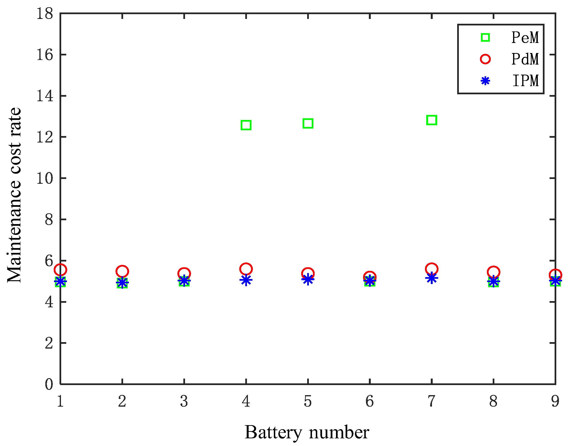
Periodic preventive maintenance strategy, which is executed when based on the historical reliability data of components. Specifically, the average failure time ${\overline{T}}_F$ of components is first obtained using the historical reliability data of multiple components, and then periodic preventive maintenance with a cost of $\left(C_p+S\right)$ is executed at time $T_R$ as follows:

$$T_R={[{\overline{T}}_F]}^{+}$$

(27)

where ${\left[x\right]}^{+}$ denotes taking the smallest integer greater than or equal to the real number x.

Since maintenance activities are planned in advance, spare parts are available at this time. Conversely, if a part fails before moment $T_R$, the part cannot arrive immediately and cannot be used for fault maintenance. In this case, fault maintenance will be performed. Therefore, the maintenance cost rate for this strategy is given by the following equation:

$${MCR}_{PeM}=\frac{C_p+S}{T_R}·\delta \left(T_F\ge T_R\right)+\frac{C_c+S}{T_F}\cdot \delta \left(T_F<T_R\right)$$

(28)

(2)

Ideal predictive maintenance strategy, which is executed based on the assumption of perfectly predicted failure times. In this case, we assume that the remaining life is accurately predicted; then, the maintenance execution moment $T_R$ should be one cycle before the actual failure moment $T_F$ of the component.

$$T_R=T_F-1$$

(29)

Then, the decision based on this perfect information will result in minimizing the value of the cost rate, which is given by the following equation:

$${MCR}_{IPM}=\frac{C_p+S}{T_R}$$

(30)

The first step involves comparing the RUL-based predictive maintenance strategy proposed in this study with the traditional state-based maintenance approach. The decision results are summarized in

Table 6. Comparative results with traditional state-based maintenance.

Maintenance Strategy	Decision-Making
	Order Spare Parts	Maintenance Activities
State-based maintenance strategy	Spare parts are not ordered	Do not perform maintenance
The maintenance strategy proposed in our paper	Predicted to order spare parts in cycle 134	Predicted to perform at cycle 144 Replacement

.

For the state-based maintenance, the decision is to perform no immediate maintenance but order parts at cycle 125 (current cycle). It is evident that the state-based approach only provides instant decisions without considering future predictions. In contrast, our proposed maintenance strategy predicts a scheduled maintenance time at cycle 144 and suggests ordering spare parts at cycle 134. Notably, for a specific component with failure expected at cycle 161, the predicted maintenance activity time aligns reasonably well.

This demonstrates that our predictive maintenance strategy accurately forecasts when preventive measures should be taken for individual components. This ability aids in the proactive planning of spare parts inventory and production activities.

Furthermore, we conducted RUL prediction using data from nine battery components and calculated the optimal moment for performing maintenance as well as the associated maintenance cost rate (MCR) for each component. We compared these results with both PeM and IPM strategies which also focus on long-term decisions. Figure 12 illustrates the MCR of these three maintenance strategies specifically applied to nine instances of #1 cells.

The figure illustrates the outcomes of our analysis, juxtaposing the proposed predictive maintenance strategy (referred to as PdM) with the periodic preventive maintenance strategy (PeM). It emphasizes that, in the majority of battery performance cases, the PdM strategy demonstrates a reduced rate of maintenance cost (MCR) in comparison to PeM.

This can be attributed to the conservative and lagged execution nature of PeM, which often leads to delayed maintenance, resulting in economic inefficiency due to a higher number of failed batteries at the time of maintenance. In contrast, our proposed strategy allows for more timely and efficient component maintenance, significantly reducing costs.

While an ideal predictive maintenance strategy (IPM) boasts the lowest MCR in theory, it is based on perfect predictive information which is not practically achievable in production settings. However, it is worth noting that our proposed strategy closely aligns with IPM in terms of MCR. Specifically, we calculated average MCR values for each approach: 7.545 for PeM, 5.433 for PdM proposed in this study, and 5.039 for IPM. These findings affirm that our proposed strategy effectively reduces single-component maintenance costs.

To further evaluate the effectiveness of our approach at a system level, we assessed three different systems comprising nine battery components. The earliest instance requiring maintenance within each system served as an opportunity for system-level scheduled maintenance. Additionally, other components falling within their respective best opportunity windows were also given scheduled opportunities for maintenance—these are detailed in

Table 7. Results of system opportunity maintenance grouping and cost rate calculations.

System	Component	${\mathit{t}}_{\mathit{R}}^{\ast }$	${\mathit{c}}_{\mathit{h}}$	$\mathbf{\Delta }{\mathit{t}}_0^{\ast }$	${\mathit{G}}_{\mathit{u}}$	${\mathit{c}}_{\mathit{s}}$	${\mathit{c}}_{\mathit{o}\mathit{s}}$	$\mathit{Q}$	$\mathit{q}$	$\mathit{v}$
1	$m$	144	30	-	$m,j,n$	16.40	12.01	670	4.65	3
	$j$	146	40	12.5
	$n$	149	50	10
2	$m$	143	30	-	$m,j$	16.16	14.57	260	1.82	2
	$j$	149	40	12.5
	$n$	154	50	10
3	$m$	143	30	-	$m,j,n$	16.33	13.71	440	3.08	3
	$j$	147	40	12.5
	$n$	151	50	10

.

Based on the data presented in the table, it is evident that implementing system-level opportunistic maintenance decisions yields substantial cost savings. Notably, Systems 1 and 3 demonstrate a remarkable outcome as all three components are grouped together and maintained simultaneously, resulting in respective savings of 670 and 440 units. In System 2, two out of the three components are included in the opportunistic maintenance combination, leading to a significant cost reduction in 260 units. This strategic approach effectively reduces overall system maintenance costs across all three systems, with System 1 showcasing the most prominent improvement.

The implementation of this strategy brings about a notable decrease in the system maintenance cost rate for System 1 from 16.40 to an impressive value of only 12.01. This reduction can be attributed to optimized prediction of maintenance timing, whereby all three components align closely within their respective opportunity maintenance windows.

When compared through calculations without opportunistically incorporating these maintenance measures, it is estimated that the average system maintenance cost amounts to approximately 2400 units at an average cost rate of around 16.30. However, by adhering to our proposed strategy involving opportunistic maintenance practices, this average cost significantly drops down to approximately 1943 units with an average cost rate reduced to only 13.43 units. This finding unequivocally demonstrates that our suggested strategy effectively minimizes fixed configuration-based maintenance costs at the system level.

Furthermore, our computations reveal that employing traditional periodic preventive maintenance would result in an average system maintenance expense of approximately 3600 units with an associated average cost rate reaching 22.63 units across all systems combined. By contrast, our novel model presents itself as highly advantageous as it slashes both the average system-wide maintenance expenses by up to 45% and diminishes the corresponding average cost rates by 40%.

In summary, based on these experimental outcomes and analyses conducted herein, this paper successfully establishes that our proposed multi-component system’s predictive RUL-based maintenance strategy proves to be a highly effective and efficient approach.

5. Conclusions

In recent years, the maintenance problem of multi-component systems has emerged as a focal point in the field of equipment health management. Numerous scholars and engineers have dedicated their efforts to exploring viable maintenance solutions. Thanks to advancements in sensing technology and artificial intelligence, the availability and usability of component degradation data have significantly improved. However, traditional approaches relying on degradation models or empirical expertise alone often yield inaccurate results and are inefficient. Therefore, it has become crucial to integrate monitoring data with degradation models for accurate prediction of remaining service life, enabling precise scheduling of maintenance time and methods.

The primary focus of this paper encompasses the following research areas:

(1)

Based on economic correlations within multi-component systems, component remaining useful life (RUL) predictions, and cost-based maintenance approaches, this study presents an integrated maintenance model that incorporates appropriate assumptions and provides a comprehensive analysis of the overall maintenance strategy. Additionally, we employ a particle-filter-based RUL prediction technique in this paper, which combines model and data-driven approaches to achieve enhanced prediction performance. This approach offers significant advantages over traditional model-based methods.

(2)

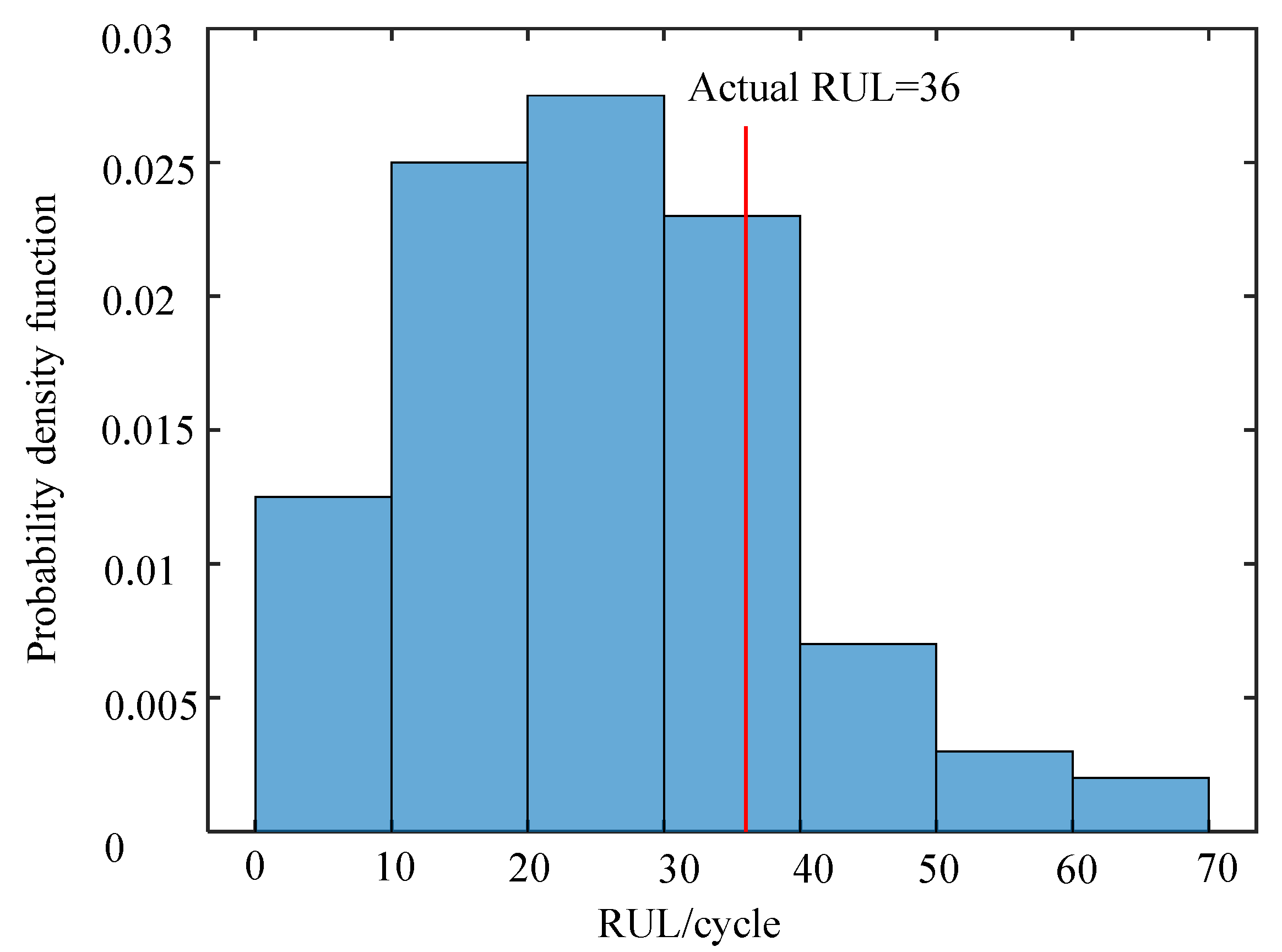
The proposed methodology is validated through an empirical analysis conducted on lithium battery group data. The findings demonstrate that the RUL prediction method presented in this paper outperforms traditional model-based methods in terms of accuracy. Furthermore, probability density function analysis offers valuable insights for determining optimal system maintenance moments. The suggested maintenance strategy allows for a more precise estimation of the optimal execution moment for opportunity-based maintenance within the system context. Compared to conventional periodic preventive measures, this approach can potentially reduce total system maintenance costs by approximately 45%.

Currently, our research does possess certain limitations. However, in the future, we plan to further advance our investigations and extend the application of the method proposed in this paper to encompass other complex systems, such as automobile engines and cranes. Simultaneously, we aim to incorporate additional influential factors into our model, such as the structural correlation between components and downtime. By doing so, we anticipate significant advancements and a promising outlook for the research presented in this paper.

References

- Zhao, W.; Lv, Y.; Liu, J.; Lee, C.K.; Tu, L. Early fault diagnosis based on reinforcement learning optimized-SVM model with vibration-monitored signals. Qual. Eng. 2023, 1–16. [Google Scholar] [CrossRef]
- Lv, Y.; Zhao, W.; Zhao, Z.; Li, W.; Ng, K.K.H. Vibration signal-based early fault prognosis: Status quo and applications. Adv. Eng. Inform. 2022, 52, 101609. [Google Scholar] [CrossRef]
- Keizer, M.C.O.; Flapper, S.D.P.; Teunter, R.H. Condition-based maintenance policies for systems with multiple dependent components: A review. Eur. J. Oper. Res. 2017, 261, 405–420. [Google Scholar] [CrossRef]
- Peng, H.; Feng, Q.; Coit, D.W. Reliability and maintenance modeling for systems subject to multiple dependent competing failure processes. IIE Trans. 2010, 43, 12–22. [Google Scholar] [CrossRef]
- Wang, J.; Zhang, X.; Zeng, J. Dynamic group-maintenance strategy for wind farms based on imperfect maintenance model. Ocean Eng. 2022, 259, 111311. [Google Scholar] [CrossRef]
- Zheng, P.; Zhao, W.; Lv, Y.; Qian, L.; Li, Y. Health Status-Based Predictive Maintenance Decision-Making via LSTM and Markov Decision Process. Mathematics 2023, 11, 109. [Google Scholar] [CrossRef]
- Liu, C.; Tang, D.; Zhu, H.; Nie, Q. A novel predictive maintenance method based on deep adversarial learning in the intelligent manufacturing system. IEEE Access 2021, 9, 49557–49575. [Google Scholar] [CrossRef]
- Kuncham, E.; Sen, S.; Kumar, P.; Pathak, H. An online model-based fatigue life prediction approach using extended Kalman filter. Theor. Appl. Fract. Mech. 2022, 117, 103143. [Google Scholar] [CrossRef]
- Guo, J.; Cai, J.; Jiang, H.; Li, X. Remaining useful life prediction for auxiliary power unit based on particle filter. Proc. Inst. Mech. Eng. Part G J. Aerosp. Eng. 2020, 234, 2211–2217. [Google Scholar] [CrossRef]
- de León Hijes, F.G.; Robles, J.S.; García, F.M.; García, M.A. Dynamic Management of Periodicity between Measurements in Predictive Maintenance. Measurement 2023, 213, 112721. [Google Scholar] [CrossRef]
- Tsao, Y.C.; Vu, T.L. Electricity pricing, capacity, and predictive maintenance considering reliability. Ann. Oper. Res. 2023, 322, 991–1011. [Google Scholar] [CrossRef]
- Chen, C.; Wang, C.; Lu, N.; Jiang, B.; Xing, Y. A data-driven predictive maintenance strategy based on accurate failure prognostics. Eksploat. Iniezawodność—Maint. Reliab. 2021, 23, 387–394. [Google Scholar] [CrossRef]
- Lv, Y.; Guo, X.; Zhou, Q.; Qian, L.; Liu, J. Predictive maintenance decision-making for variable faults with non-equivalent costs of fault severities. Adv. Eng. Inform. 2023, 56, 102011. [Google Scholar] [CrossRef]
- Bouabdallaoui, Y.; Lafhaj, Z.; Yim, P.; Ducoulombier, L.; Bennadji, B. Predictive Maintenance in Building Facilities: A Machine Learning-Based Approach. Sensors 2021, 21, 1044. [Google Scholar] [CrossRef]
- Orth, P.; Yacout, S.; Adjengue, L. Accuracy and robustness of decision making techniques in condition based maintenance. J. Intell. Manuf. 2012, 23, 255–264. [Google Scholar] [CrossRef]
- Huynh, K.T.; Grall, A.; Bérenguer, C. Assessment of diagnostic and prognostic condition indices for efficient and robust maintenance decision-making of systems subject to stress corrosion cracking. Reliab. Eng. Syst. Saf. 2017, 159, 237–254. [Google Scholar] [CrossRef]
- Wang, H.; Lin, D.; Qiu, J.; Ao, L.; Du, Z.; He, B. Research on Multiobjective Group Decision-Making in Condition-Based Maintenance for Transmission and Transformation Equipment Based on D-S Evidence Theory. IEEE Trans. Smart Grid 2015, 6, 1035–1045. [Google Scholar] [CrossRef]
- Lin, L.; Luo, B.; Zhong, S. Development and application of maintenance decision-making support system for aircraft fleet. Adv. Eng. Softw. 2017, 114, 192–207. [Google Scholar] [CrossRef]
- Vališ, D.; Žák, L.; Pokora, O.; Lánský, P. Perspective analysis outcomes of selected tribodiagnostic data used as input for condition based maintenance. Reliab. Eng. Syst. Saf. 2016, 145, 231–242. [Google Scholar] [CrossRef]
- Zhang, C.; Qi, F.; Zhang, N.; Li, Y.; Huang, H. Maintenance policy optimization for multi-component systems considering dynamic importance of components. Reliab. Eng. Syst. Saf. 2022, 226, 108705. [Google Scholar] [CrossRef]
- Sheikhalishahi, M.; Azadeh, A.; Pintelon, L. Dynamic maintenance planning approach by considering grouping strategy and human factors. Trans. Inst. Chem. Eng. Process Saf. Environ. Prot. Part B 2017, 107, 289–298. [Google Scholar] [CrossRef]
- Van, P.D.; Barros, A.; Bérenguer, C.; Bouvard, K.; Brissaud, F. Dynamic grouping maintenance with time limited opportunities. Reliab. Eng. Syst. Saf. 2013, 120, 51–59. [Google Scholar] [CrossRef]
- Vu, H.C.; Do, P.; Barros, A.; Bérenguer, C. Maintenance grouping strategy for multi-component systems with dynamic contexts. Reliab. Eng. Syst. Saf. 2014, 132, 233–249. [Google Scholar] [CrossRef]
- Do, P.; Vu, H.C.; Barros, A.; Bérenguer, C. Maintenance grouping for multi-component systems with availability constraints and limited maintenance teams. Reliab. Eng. Syst. Saf. 2015, 142, 56–67. [Google Scholar] [CrossRef]
- Vu, H.C.; Do, P.; Barros, A. A study on the impacts of maintenance duration on dynamic grouping modeling and optimization of multicomponent systems. IEEE Trans. Reliab. 2018, 67, 1377–1392. [Google Scholar] [CrossRef]
- de Pater, I.; Mitici, M. Predictive maintenance for multi-component systems of repairables with Remaining-Useful-Life prognostics and a limited stock of spare components. Reliab. Eng. Syst. Saf. 2021, 214, 107761. [Google Scholar] [CrossRef]
- Alhourani, F.; Essila, J.; Farkas, B. Preventive maintenance planning considering machines’ reliability using group technology. J. Qual. Maint. Eng. 2023, 29, 136–154. [Google Scholar] [CrossRef]
- Carvalho, T.P.; Soares, F.A.; Vita, R.; Francisco, R.D.P.; Basto, J.P.; Alcalá, S.G. A systematic literature review of machine learning methods applied to predictive maintenance. Comput. Ind. Eng. 2019, 137, 106024. [Google Scholar] [CrossRef]
- Chang, F.; Zhou, G.; Zhang, C.; Xiao, Z.; Wang, C. A service-oriented dynamic multi-level maintenance grouping strategy based on prediction information of multi-component systems. J. Manuf. Syst. 2019, 53, 49–61. [Google Scholar] [CrossRef]
- Gorenstein, A.; Kalech, M. Predictive maintenance for critical infrastructure. Expert Syst. Appl. 2022, 210, 118413. [Google Scholar] [CrossRef]
- Shi, H.; Zeng, J. Real-time prediction of remaining useful life and preventive opportunistic maintenance strategy for multi-component systems considering stochastic dependence. Comput. Ind. Eng. 2016, 93, 192–204. [Google Scholar] [CrossRef]
- Nguyen, K.T.; Medjaher, K. A new dynamic predictive maintenance framework using deep learning for failure prognostics. Reliab. Eng. Syst. Saf. 2019, 188, 251–262. [Google Scholar] [CrossRef]